The Anomalous Magnetic Moment of a photon propagating in a magnetic field

Abstract

We analyze the spectrum of the Hamiltonian of a photon propagating in a strong magnetic field $B\sim B_{\rm{cr}}$, where $B_{\rm cr}=\frac{m^{2}}{e}\simeq 4.4\times 10^{13}$ Gauss is the Schwinger critical field . We show that the expected value of the Hamiltonian of a quantized photon for a perpendicular mode is a concave function of the magnetic field $B$. We show by a partially analytic and numerical method that the anomalous magnetic moment of a photon in the one loop approximation is a non - decreasing function of the magnetic field $B$ in the range $0\leq B\leq 30\,B_{\rm cr}$ We provide a numerical representation of the expression for the anomalous magnetic moment in terms of special functions. We find that the anomalous magnetic moment $\mu_{\gamma}$ of a photon for $B=30\,B_{\rm cr}$ is $8/3$ of the anomalous magnetic moment of a photon for $B=1/2~{}B_{\rm cr}$.

1 Introduction

The nonlinearity of Maxwell’s wonderful equations continues to present and challenge us with a variety of interesting phenomenon. The effective interaction that results due to the corrections from the virtual excitations of the charged quantum fields, such as electron $e^{-}$ and positron $e^{+}$, leads to well known interesting effects (Dittrich & Gies, 2000). More recently, other interesting aspects of the quantum vacuum have been explored by Shabad & Usov (2011); Villalba-Chávez & Shabad (2012); Altschul (2008) to name but a few. In the case of electromagnetic fields that vary slowly with respect to the Compton wavelength, i.e. frequencies much less than the pair creation threshold, the one loop quantum electrodynamic effective Heisenberg-Euler Lagrangian (HEL), McKeon (1979); Shabad & Usov (2011); Villalba-Chávez & Shabad (2012); Dunne (2004) describes the dominant physical effects. The HEL is known to all orders in electromagnetic fields. It is well known that electrons acquire an anomalous magnetic moment due to the radiative corrections in quantum electrodynamics (QED) with the $e^{-}-e^{+}$ pairs and virtual photons in the background (Schwinger, 1951). It is also of great fundamental interest that there is an anomalous photon magnetic moment $\mu_{\gamma}$ due to the interaction with the external magnetic field in the environment of the virtual $e^{-}-e^{+}$ quanta of the vacuum. The last couple of decades has seen a resurgence of interest in quantum vacuum physics (Gies, 2008; Baring, 1995; Mielniczuk et al., 1988; Heyl & Hernquist, 1997b, a, c; Dunne, 2009).The promise of high intensity experimental facilities ($\sim 10^{15}$ W) has stimulated immense interest and enthusiasm to investigate the nonlinear quantum vacuum in practical optical experiments (Marklund & Shukla, 2006; Dunne, 2009; Della Valle et al., 2013, 2014). The Polarization of the Vacuum with Laser (PVLAS) experiment aims to measure the birefringence of the external magnetic field in the vacuum (Zavattini et al., 2008; Bregant, 2008; Cantatore, 2008).

In section 2, we outline and discuss the analytic calculations on the anomalous magnetic moment of the photon. We present and discuss the results. In section 3 we briefly outline the mathematical expression for the photon center of mass and the expression for the group velocity. Section 4 presents the conclusions. The supplementary mathematical details are provided in appendices A, B and C.

2 Anomalous Magnetic Moment of a Photon

Villalba-Chávez (2010); Villalba-Chávez & Shabad (2012) and Rojas & Querts (2006, 2007) have discussed the notion of the anomalous magnetic moment of a photon . The photon anomalous magnetic moment and its paramagnetic properties that have been studied by Pérez Rojas & Rodríguez Querts (2014); Rojas & Querts (2006, 2007) have provided values of $\mu_{\gamma}$ in the two extreme limits of $B\ll B_{\rm cr}$ and $B\gg B_{\rm cr}$. The purpose of this paper is to provide numerical values and an analytic formula for the range $B\sim B_{\rm cr}$. Our results are applicable in the range $0\leq B\leq 30\,B_{\rm cr}$.

At one-loop order, the Heisenberg Euler effective Lagrangian in constant external electromagnetic fields (Heisenberg & Euler, 1936; Karbstein & Shaisultanov, 2015), describing the effective nonlinear interactions between the electromagnetic fields mediated by electron-positron fluctuations in the vacuum, can be represented concisely in terms of the following proper time integral (Schwinger, 1951).

$$\mathcal{L}=\frac{\alpha}{2\pi}\int_{0}^{\infty}\frac{ds}{s}e^{{-i\frac{m^{2}}{e}s}}\left[ab\coth(as)\cot(bs)-\frac{a^{2}-b^{2}}{3}-\frac{1}{s^{2}}\right]$$ (1)

with the prescription $m^{2}\rightarrow m^{2}-\i 0^{+}$, and the proper time integration contour assumed to lie slightly below the real positive $s$ axis. Here, m is the electron mass, $e$ is the elementary charge, $\alpha=\frac{e^{2}}{4\pi}$ is the fine structure constant, and $a=(\sqrt{\mathcal{F}^{2}+\mathcal{G}^{2}}-\mathcal{F})^{1/2}$ and $b=(\sqrt{\mathcal{F}^{2}+\mathcal{G}^{2}}+\mathcal{F})^{1/2}$ are the secular invariants made up of the gauge and Lorentz invariants of the electromagnetic field: $\mathcal{F}=\frac{1}{4}F_{\mu\nu}F^{\mu\nu}=\frac{1}{2}(\textbf{B}^{2}-\textbf{E}^{2})$ and $\mathcal{G}=\frac{1}{4}F^{*}_{\mu\nu}F^{\mu\nu}=-\textbf{E}\cdot\textbf{B}$, with ${}^{*}F^{\mu\nu}=\frac{1}{2}\epsilon^{\mu\nu\alpha\beta}F_{\alpha\beta}$ denoting the dual field strength tensor; $\epsilon^{\mu\nu\alpha\beta}$ is the totally antisymmetric tensor, fulfilling $\epsilon^{0123}=1$. Our metric convention is $g_{\mu\nu}=diag(-1,+1,+1,+1)$, and we use the units where $c=\hbar=1$. To keep notations compact we moreover employ the short hand notations $\int_{x}\equiv\int d^{4}x$ and $\int_{k}\equiv\int\frac{d^{4}k}{(2\pi)^{4})}$ for the integration over the position and the momentum space, respectively.

The seminal paper of Schwinger (1951) on gauge invariance and vacuum polarization has used the proper time parameter formulation to the solution of the equation of motion of a particle. Thereby, the effective Lagrangian (Karbstein & Shaisultanov, 2015) is finite, gauge and Lorentz invariant. The derivative expansion of the one loop effective Lagrangian in QED has been studied by Gusynin & Shovkovy (1996). Their non-perturbative term is that derived by Schwinger but the second term in their expansion shows explicitly the two derivatives of $F_{\mu\nu}$ that account the case where the fields are slowly or fast varying. We do not consider them now in the assumption of the constant field approximation but the effects of additional terms to the Schwinger Lagrangian warrant a more detailed analysis in a further study. If the typical frequency/momentum scale of the variation of the homogeneous background field is $\nu$, derivatives effectively translate into multiplications with $\nu$ to be rendered dimensionless by the electron mass $m$. Thus, Equation 1 is also applicable for slowly varying inhomogeneous fields fulfilling $\frac{\nu}{m}\ll 1$, or in other words for inhomogeneities whose typical spatial (temporal) scales of variation are much larger than the Compton wavelength (time) $\sim\frac{1}{m}$ of the virtual charged particle. The electron Compton wavelength is $\lambda_{c}=3.86\times 10^{-13}$ m and the Compton time is $\tau_{c}=1.29\times 10^{-21}$ s. In turn, many electromagnetic fields available in the laboratory, e.g., the electromagnetic field pulses generated by optical high intensity lasers, (Dunne, 2009) featuring wavelengths of $\mathcal{O}(\mu m)$ and pulse durations of $\mathcal{O}(fs)$, are compatible with this requirement.

The effective Lagrangian is a scalar quantity, and the scalar quantities made up of combinations of $F^{\mu\nu}$, ${}^{*}F^{\mu\nu}$, and the derivatives thereof involve an even number of derivatives. Hence, when employing the constant fields results (Karbstein & Shaisultanov, 2015) for the slowly varying inhomogeneous field, the derivations from the corresponding exact results are of $\mathcal{O}((\frac{\nu}{m})^{2})$. In the absence of an external electric field the partial derivatives of the effective action in the one loop approximation are (Lundin, 2009, 2010)

$$\gamma_{\mathcal{F}}=\frac{\partial\mathcal{L}}{\partial{\mathcal{F}}},\gamma_{\mathcal{F}\mathcal{F}}=\frac{\partial^{2}\mathcal{L}}{\partial\mathcal{F}^{2}},\gamma_{\mathcal{G}\mathcal{G}}=\frac{\partial^{2}\mathcal{L}}{\partial\mathcal{G}^{2}}.$$ (2)

Expressions such as $\gamma_{\mathcal{G}}$, $\gamma_{\mathcal{F}\mathcal{G}}$ are zero for zero electric field. Further,

$$\gamma_{\mathcal{F}}=-1-\frac{\alpha}{2\pi}[\frac{1}{3}+2h^{2}-8\zeta^{\prime}(-1,h)+4h\ln\Gamma(h)-2h\ln h+\frac{2}{3}\ln h-2h\ln 2\pi]$$ (2a)

$$\gamma_{\mathcal{F}\mathcal{F}}=\frac{\alpha}{2\pi{B^{2}}}[\frac{2}{3}+4h^{2}\psi(1+h)-2h-4h^{2}-4h\ln\Gamma(h)+2h\ln 2\pi-2h\ln h]$$ (2b)

$$\gamma_{\mathcal{G}\mathcal{G}}=\frac{\alpha}{2\pi B^{2}}\left[-\frac{1}{3}-\frac{2}{3}\psi(1+h)-2h^{2}+(3h)^{-1}+8\zeta^{\prime}(-1,h)-4h\ln\Gamma(h)+2h\ln(2\pi)+2h\ln h\right]$$ (2c)

where $\psi$ is the digamma function, $\Gamma$ is the gamma function, and $h=\frac{1}{2}\frac{B_{\rm c}}{B}$.

$$\gamma_{\mathcal{G}\mathcal{G}}=\frac{\partial^{2}\mathcal{L}}{\partial\mathcal{G}^{2}}\arrowvert_{\mathcal{F}=\frac{1}{2}B^{2}}^{\mathcal{G}=0}$$ (3)

Also

$$\zeta^{\prime}(s,h)=\partial_{s}\zeta(s,h),$$ (4)

where $\zeta(s,h)$ is the Hurwitz zeta function, for $s=-1$ given by Adamchik (2004) and $h>>1$ (Dittrich, 1979)

$$\zeta^{\prime}(-1,h)\cong\frac{1}{12}-\frac{h^{2}}{4}+\frac{\ln h}{2}(h^{2}-h+\frac{1}{6})+\int^{\infty}_{0}\frac{e^{-hx}}{x^{2}}(\frac{1}{1-e^{-x}}-\frac{1}{x}-\frac{1}{2}-\frac{x}{12})dx,\,\,\,Re(h)>0$$ (5)

$$\zeta^{\prime}(-1,h)\cong\frac{1}{12}-\frac{h^{2}}{4}+\frac{\ln h}{2}(B_{2}(h))+\frac{1}{720}\frac{1}{h^{2}}.$$ (6)

where $B_{2}(h)=h^{2}-h+\frac{1}{6}$ is the second Bernoulli polynomial (Olver et al., 2010). The integral above is convergent (Adamchik, 2004).

The refractive indices for perpendicular and parallel polarized photons are of particular interest in this context. It is worth noting that

$$\frac{4\pi}{\alpha}(n_{\perp}-1)=\frac{2\pi{B}^{2}}{\alpha}\gamma_{\mathcal{G}\mathcal{G}},$$ (7)

where $\gamma_{\mathcal{G}\mathcal{G}}$ has been defined in Equation 2c. For the weak field case, $n_{\perp}$ is given by the expression (Heyl & Hernquist, 1997b, a, c). $\xi=\frac{B}{B_{cr}}=\frac{1}{2h}$ and $\xi<1$

$$n_{\perp}=1+\frac{\alpha}{4\pi}\sin^{2}\theta\left[\frac{14}{45}\xi^{2}-\frac{1}{3}\sum_{j=2}^{\infty}\frac{2^{2j}(6B_{2(j+1)}-(2j+1)B_{2j})}{j(2j+1)}\xi^{2j}\right]+\mathcal{O}\left[\left(\frac{\alpha}{2\pi}\right)^{2}\right]$$ (8)

where $\xi=\frac{B}{B_{\rm cr}}$, $\alpha$ is the fine structure constant, $B_{2j}$ and $B_{2j+1}$ are the Bernoulli numbers. In the strong-field limit $(\xi>0.5)$, we obtain

$$n_{\perp}=1+\frac{\alpha}{4\pi}\sin^{2}\theta[\frac{2}{3}\xi-\left(8\ln A-\frac{1}{3}-\frac{2}{3}\gamma\right)-\left(\ln\pi+\frac{1}{18}\pi^{2}-2-\ln\xi\right)\xi^{-1}$$ (9)

$$-\left(-\frac{1}{2}-\frac{1}{6}\zeta(3)\right)\xi^{-2}-\sum_{j=3}^{\infty}\frac{(-1)^{j-1}}{2^{j-2}}\left[\frac{j-2}{j(j-1)}\zeta(j-1)+\frac{1}{6}\zeta(j+1)\xi^{-j}\right]+\mathcal{O}\left[\left(\frac{\alpha}{2\pi}\right)^{2}\right]$$ (10)

For parallel polarizations, the refractive index is given by Tsai & Erber (1975)

$$n_{\parallel}=1+\frac{\alpha}{4\pi}[-\frac{1}{3}-\frac{2}{3}\psi(1+h)+8\zeta^{\prime}(-1,h)-2h^{2}+\frac{1}{3h}-4h\ln\Gamma(h)+2h\ln(2\pi)+2h\ln h].$$ (11)

which is valid for all $B\leq\frac{\pi}{\alpha}B_{cr}$.

$$\Delta{n}_{\perp,\parallel}=n_{\perp}-n_{\parallel}=\frac{\alpha}{4\pi}[\frac{1}{3h}-(8\ln A-\frac{1}{3}-\frac{2}{3}\gamma)-2h(\ln\pi+\frac{\pi^{2}}{18}-2+\ln 2h)$$

$$+2h^{2}+\frac{2}{3}\zeta(3)h^{2}-\sum_{j=3}^{\infty}\frac{(-1)^{j-1}}{2^{j-2}}+\{(j-2)+\frac{\zeta(j+1)}{6}+\frac{h^{j}}{2j}\}+\frac{2}{3}\ln(1+h)-\frac{1}{3}\frac{1}{1+h}-\frac{2}{3}-\frac{2}{3}\ln h-\frac{22}{48}\frac{1}{h^{2}}]$$

Here $\zeta$ is the Riemann zeta function, $\zeta(3)\cong 1.202$, $\theta$ is the angle between the magnetic field B and the vector k, $\gamma\cong 0.577$ which is the Euler-Mascheroni constant and $A\cong 1.28242712...$ is the Glaisher-Kinkelin constant (Olver et al., 2010).

An important physical variable is the Faraday rotation angle $\chi$ as $\chi=k(n_{\perp}-n_{\parallel})l$, where $k$ is the magnitude of the photon wave vector and $l$ can be viewed as the path distance of the photon in the magnetic field. The Faraday rotation can, in principle, be observable for appreciable values of k and $l$ .

We will analyze the properties of a photon propagating in a strong magnetic field B. The Hamiltonian of a photon is given by (Bialynicki-Birula & Bialynicka-Birula, 2012; Bialynicka-Birula & Bialynicki-Birula, 2014)

$$\hat{H}(B)=\sum_{\lambda}\int d^{3}k\,\hbar\omega_{k}a^{\dagger}_{\lambda}(\textbf{k})a_{\lambda}(\textbf{k})$$ (13)

where the creation and the annihilation operator satisfy the commutation rule

$$[a^{\dagger}_{\lambda}(\textbf{k}),a_{\lambda^{\prime}}(\textbf{k}^{\prime})]=\delta_{{\lambda},{\lambda^{\prime}}}\delta(\textbf{k}-\textbf{k}^{\prime})$$ (14)

From the linearity in the term proportional to $\mu_{\gamma}$ of the Hamiltonian (Villalba-Chávez & Shabad, 2012; Pérez Rojas & Rodríguez Querts, 2014).

$$\mu_{\gamma}=-\frac{d\langle\hat{H}(\textbf{B})\rangle}{dB}$$ (15)

where $\mu_{\gamma}$ denotes the magnetic moment and $\langle\rangle$ denotes the quantum expectation value for a perpendicularly polarized photon. We have

$$\omega_{\parallel}=\frac{|\textbf{k}|}{n_{\parallel}}$$ (16)

$$\omega_{\perp}=\frac{|\textbf{k}|}{n_{\perp}}$$ (17)

$\omega_{\parallel}$ and $\omega_{\perp}$ are the photon frequencies in the parallel and the perpendicular modes and the corresponding indices of refraction are

$$n_{\parallel}=\frac{1}{\sqrt{1-\kappa_{s}\sin^{2}\theta}}$$ (18)

$$n_{\perp}=\sqrt{\frac{1+\kappa_{p}}{1+\kappa_{s}\cos^{2}\theta}}$$ (19)

where $\kappa_{s}$ and $\kappa_{p}$ are given below by equations (21) and (26). For $\theta=\frac{\pi}{2}$ we have

$$n_{\perp}=\sqrt{1+\kappa_{p}}$$ (20)

$$\kappa_{s}=\gamma_{\mathcal{F}\mathcal{F}}\frac{B^{2}}{\gamma_{s}}.$$ (21)

$$\gamma_{s}=1-\gamma_{\mathcal{F}}$$ (22)

Using the binomial expansion, $n_{\parallel}$ can be approximately written as

$$n_{\parallel}=1-\frac{1}{2}B^{2}\gamma_{\mathcal{F}\mathcal{F}}.$$ (23)

we will approximate

$$\frac{1}{n_{\perp}}=\frac{1}{\sqrt{1+\kappa_{p}}}\cong 1-\frac{1}{2}\kappa_{p}$$ (24)

and $\gamma_{s}\cong 1$. So

$$\langle H(B)\rangle\cong\ \langle H(0)\rangle-\frac{1}{2}B^{2}\gamma_{\mathcal{G}\mathcal{G}}$$ (25)

$$\kappa_{p}=\gamma_{\mathcal{G}\mathcal{G}}B^{2}/\gamma_{s}$$ (26)

Following Bialynicki-Birula & Bialynicka-Birula (2012); Bialynicka-Birula & Bialynicki-Birula (2014) we will call the mode perpendicular if the magnetic field of the photon is in the plane formed by the vectors B and k where k is the wave vector of the photon. In the approximation

$$\frac{1}{\sqrt{1+\kappa_{p}}}\cong 1-\frac{1}{2}\kappa_{p}$$ (27)

and $\gamma_{s}\cong 1$ we will confine ourselves to the range $0\leq B\leq\,B_{\rm cr}$. The radiative corrections come into visible play for $B\geq 430B_{\rm cr}$. As an aside, it is interesting to note that although the equation of motion of a neutrino in an external magnetic field is effectively altered (McKeon, 1981), the radiative correction effects on a neutrino beam by a strong magnetic field is $2\times 10^{10}T$ have been found to be extremely small.

We define

$$\gamma_{\mathcal{F}\mathcal{F}}=\frac{\partial^{2}\mathcal{L}}{\partial\mathcal{F}^{2}}\arrowvert_{\mathcal{F}=\frac{1}{2}B^{2}}^{\mathcal{G}=0}$$ (28)

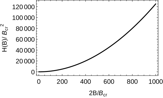
Figure 1: Shows the expression of the Hamiltonian given in 25 as a function of the magnetic field B. The vertical and the horizontal axis are normalized in units of $B_{cr}^{2}$ and $B_{cr}$, respectively.

Fig.(1) illustrates that $\langle H(B)\rangle$ is a convex function of the magnetic field B. The numerical results of Fig. (1) were obtained by Mathematica 10. Fig.(1) illustrates that $\langle H(B)\rangle$ is a increasing function of the magnetic field.

From equations 15 and 25 the photon magnetic moment of a perpendicularly polarized photon for $B\leq 30B_{\rm cr}$ and the fact that $\mu_{\gamma}(0)=0$, is given by

$$\mu_{\gamma}(B)=\frac{\alpha}{4\pi}\left\{\frac{2}{3}+\frac{1}{B^{3}}\left[\frac{1}{3}B\psi^{\prime}\left(1+\frac{1}{2B}\right)+\psi\left(\frac{1}{2B}\right)-2B\ln\Gamma\left(\frac{1}{2B}\right)+B\ln(2\pi)+B+B\ln(2B)-1)\right]\right\}\left(\frac{|\textbf{k}|}{m}\right)\sin^{2}\theta$$ (29)

where $\psi$ is the digamma function, $\Gamma$ is the Euler gamma function. From equation (29), one observes that the photon magnetic moment contributes to both the external field strength as well as the photon energy through its momentum.

For $B>\frac{1}{2}B_{\rm cr}$ we can approximate

$$\mu_{\gamma}(B)\cong\frac{\alpha}{4\pi}\left[\frac{2}{3}+\left(\ln(\pi)+\frac{\pi^{2}}{18}-1\right)B^{-2}-\frac{\ln B}{B^{2}}\right]\left(\frac{|\textbf{k}|}{m}\sin^{2}\theta\right)$$ (30)

where k is the photon wave vector.

It is interesting to note that rearrangement of equation (30) with the terms involving $B$ and setting $c_{1}=\rm{ln}\pi+\frac{\pi^{2}}{18}-1$ gives the following equivalent expression of $\rm{ln}B$:

$$2(c_{1}-\rm{ln}B)=W_{j}\left(\left\{-\frac{8\pi}{\alpha}\frac{m}{|k|sin^{2}\theta}\mu_{\gamma}(B)+\frac{4}{3}\right\}\ {e^{2^{c_{1}}}}\right),$$ (31)

where $W_{j}$ denotes the $j$th branch of the multivalued inverse function known as the Lambert W function (Valluri et al., 2000). The Lambert W function is defined such that (Corless et al., 1996)

$$W(z)e^{W(z)}=z,$$ (32)

where $z$ can be a complex variable. The utility of this function in QED is an aspect that warrants study, although it has found many remarkable applications in a multitude of diverse fields (Corless et al., 1996; Valluri et al., 2009; Roberts & Valluri, 2016)

For $0\leq B\leq 0.44B_{\rm cr}$

$$\mu_{\gamma}(B)\cong\frac{\alpha}{4\pi}\frac{28}{45}\left(B-\frac{52}{49}B^{3}\right)\left(\frac{|\textbf{k}|}{m}\sin^{2}\theta\right).$$ (33)

For a perpendicularly polarized photon, we note that equation (33) can be replaced by the inequality

$$\mu_{\gamma}(B)\geq\frac{\alpha}{4\pi}\frac{28}{45}\left(B-\frac{52}{49}B^{3}\right)\left(\frac{|\textbf{k}|}{m}\sin^{2}\theta\right)$$ (34)

We restrict equation (29) to $0\leq B\leq 30B_{\rm cr}$. Using equation (30) we obtain that $\mu_{\gamma}(B=30B_{\rm cr})$ is only $3\%$ smaller than the asymptotic value $\alpha/(3\pi)$ of the Bohr magneton. It is approximately $10^{-3}$ of the Bohr magneton for $|\textbf{k}|\sim m$. $\mu_{\gamma}(B)$ grows from the value of

$$\frac{\alpha}{4\pi}\frac{28}{45}\frac{3}{4}\frac{1}{2}\frac{|\textbf{k}|}{m}\sin^{2}\theta$$ (35)

for $B=\frac{1}{2}B_{\rm cr}$ to the value very close to

$$\frac{\alpha}{4\pi}\frac{2}{3}\frac{|\textbf{k}|}{m}\sin^{2}\theta,$$ (36)

for $B=30B_{cr}$ so the growth is only by a factor of $\approx 3$ . Equation 30 is the generalization of equation (157) of Villalba-Chávez & Shabad (2012), who state that

$$\mu_{\gamma}(B)\sim\frac{\alpha}{3\pi}\left(\frac{1}{2}\frac{e}{m}\right),$$ (37)

for large values of the magnetic field B. This suggest that the one loop approximation provides a good estimate of $\mu_{\gamma}$ in the low frequency case. Here $e$ denotes the electron charge and m is the corresponding mass. At low and high photon frequency Villalba-Chávez & Pérez-Rojas (2006) have shown that the photon magnetic moment shows a paramagnetic behavior as is also true for the vacuum embedded in a strong external magnetic fields (Mielniczuk et al., 1988). Our equation 33 is similar to equation 19 of Pérez Rojas & Rodríguez Querts (2014) except that our numerical factor $\frac{28}{45}$ is twice bigger than their corresponding factor $\frac{14}{45}$ . Formally our equation is applicable only when

$$\frac{|\textbf{k}|}{m}\ll 1$$ (38)

Equations (29) and (30) are the main results of our paper. We will show analytically in Appendices A and B that

$$\mu_{\gamma}(B)>0\,\,\rm{for}\,\,\,B>0.$$ (39)

As was previously shown by Pérez Rojas & Rodríguez Querts (2014),

$$\frac{d}{dB}\mu_{\gamma}(B)>0\,\,\rm{for}\,\,\,B>0$$ (40)

in the two ranges $0\leq B\leq\frac{1}{2}B_{\rm{cr}}$ and $2\leq B$. Equation 40 has been checked for all positive values of $B$.

$$\mu_{\gamma}(B)=\frac{\alpha}{4\pi}\left\{\frac{2}{3}+\frac{1}{B^{3}}\left\{\left[\frac{2}{3}B\zeta\left(2,1+\frac{1}{2B}\right)-\zeta\left(1,1+\frac{1}{2B}\right)\right\}-2B\ln\Gamma\left(\frac{1}{2B}\right)+B\left(\ln(2\pi)+1-\ln\left(\frac{1}{2B}\right)\right)-1\right]\right\}.$$ (41)

where $\zeta$ is the Hurwitz zeta function. The magnetic moment can be expressed in terms of other special functions. The paramagnetic behaviour is a physical effect due to the effect of the external magnetic field on the virtual $e^{-}-e^{+}$ pairs.

3 Photon Center of Mass

The speed $v_{\rm cm}$ of the center of mass is proportional to $1-\frac{1}{2}B^{2}_{\mathcal{LGG}}$. The magnetic moment of the photon plays the leading role in determining the evolution of the photon angular momentum (Pryce, 1935; Villalba-Chávez & Shabad, 2012). The average of the corresponding center of mass location of a photon can be analyzed using the operator

$$\hat{R}=\frac{1}{2\hat{H}}\hat{N}+\hat{N}\frac{1}{2\hat{H}}$$ (42)

The Hamiltonian $\hat{H}$ of Hawton & Baylis (2001, 2005) is originally the Hamiltonian of a free photon. It will be replaced by our Hamiltonian $\hat{H}(B)$.

For brevity we keep the same symbol,

$$\hat{N}=\int d^{3}r\,\textbf{r}\,\epsilon(\textbf{r},t)$$ (43)

where $\hat{N}$ is the first moment of the energy distribution.

$$\hat{\epsilon}(\textbf{r},t)=\hat{F}^{\dagger}(\textbf{r,t})\hat{F}(\textbf{r,t})$$ (44)

$$\hat{F}(\textbf{r},t)=\frac{\hat{D}(\textbf{r},t)}{\sqrt{2\epsilon}}+i\frac{\textbf{B({r},t)}}{\sqrt{2\mu}}$$ (45)

$$x_{\rm cm}=\frac{1}{\rho^{o}}\int d^{3}x\textbf{x}\Theta^{oo}$$ (46)

and the corresponding velocity is the velocity of energy transport

$$v_{\rm cm2}=\frac{1}{u_{2}}\textbf{n}-\frac{2\mathcal{F}\mathcal{L}\_{\mathcal{G}\mathcal{G}}}{\epsilon_{||}u_{2\perp}}$$ (47)

The group velocity is less than that of the speed of light $c$, in accord with the principle of causality (Villalba-Chávez & Shabad, 2012), with $u_{\lambda\perp}=\frac{\rho^{o}(\lambda)}{|\rho(\lambda)|}$. Here $\Theta^{oo}$ and $\rho^{o}$ are given by equations (52) and (58) of the paper by Villalba-Chávez & Shabad (2012). The speed of a perpendicularly polarized photon is found to be (c=1),

$$v_{\perp}^{2}=\frac{1}{n_{\perp}^{2}}\\ \geq\frac{1}{\left(1+\frac{\alpha}{4\pi}\left(\frac{2}{3}-2h\ln h+2h\ln(2\pi)\right)\right)^{2}}.$$ (48)

In the limit of ultra strong magnetic fields, the expression of $v_{\perp}^{2}$ when ${\theta}=\frac{\pi}{2}$, derived by Hu & Liu (2007) is given below.

$$v_{\perp}^{2}\simeq\frac{1-\frac{e^{2}}{12\pi^{2}}(\ln\left(\frac{eB}{m^{2}}\right)-0.79)}{1-\frac{e^{2}}{12\pi^{2}}(\ln\left(\frac{eB}{m^{2}}\right)-1.79)}.$$ (49)

4 Conclusions

We have shown that the anomalous magnetic moment of a photon for $B=30B_{\rm cr}$ is $8/3$ of the anomalous magnetic moment of a photon for $B=\frac{1}{2}B_{\rm cr}$. At low and high photon frequencies the photon magnetic moment shows a paramagnetic behavior. We find that the one loop Lagrangian is a good approximation in the range of magnetic fields considered. We have shown that the anomalous magnetic moment of a photon is a non-decreasing function of the magnetic field B for $0\leq B\leq 30B_{\rm cr}$.

The photon behaves like a massive pseudo vector particle under the influence of the virtual $e^{-}-e^{+}$ vacuum (Villalba-Chávez & Shabad, 2012; Pérez Rojas & Rodríguez Querts, 2014). Light propagation in the magnetized vacuum is analogous to the dispersion of light in an anisotropic medium. The reason for the anisotropy is due to the breaking of symmetry due to the choice of B along a preferred direction. The magnetic moment of the photon might have both astrophysical and cosmological consequences. In the presence of magnetic fields around astrophysical objects such as magnetars, magnetic lensing may be a strong observable effect.

Photons that go by a strongly magnetized star would undergo an deflection besides the well known gravitational shift caused by the stellar mass (Villalba-Chávez & Pérez-Rojas, 2006). The Cosmic Microwave Background (CMB) spectrum shows a substantial polarization dependent field in the vicinity of magnetars (Bialynicka-Birula & Bialynicki-Birula, 2014). Bialynicka-Birula & Bialynicki-Birula (2014) have estimated the polarization dependent heating of the cosmic microwave background (CMB) radiation due to strong magnetic fields. Although the large magnetic fields around the region of magnetars is appreciable, the estimated distortion of the CMB due to the increase in temperature $T$ cannot be detected with the current detector sensitivity. It is possible that further improvements in estimated angular resolutions as well as in the precision of the temperature fluctuation measurements and experimental facilities such as the Large Hadron Collider (LHC) will make such effects as well as those of the photon anomalous magnetic moment observable.

There has been a surge of interest to investigate quantum nonlinearity in state of the art optical experimental setups (Marklund & Shukla, 2006). The QED vacuum in an external field will reveal further interesting insights into processes such as electro-gravitational conversion (Papini & Valluri, 1977). It will illuminate our further understanding of Lorentz Symmetry Breaking (LSB) in nonlinear electrodynamics (Villalba-Chávez & Shabad, 2012). Some of the strongest magnetic fields in the universe are expected to exist around magnetars (Olausen & Kaspi, 2014; Bassa et al., 2008; Olausen & Kaspi, 2014). A strong magnetic field exists around the center of the galaxy (Eatough et al., 2013). These objects with such strong magnetic fields, although contained in regions small relative to the cosmos, can still provide us with possibilities of observing nonlinear effects such as birefringence that can provide a handle to estimate physical quantities such as the photon anomalous magnetic moment and Faraday rotation (Eatough et al., 2013). Proposals have been given to search for birefringence with the use of the time varying electromagnetic fields and high precision interferometry (Grote, 2015; Zavattini & Calloni, 2009).

As long as the spatial and time inhomogeneitics are much larger than the Compton wavelength, the constant field approximation results will be reasonably accurate. More refined experimental observations of vacuum birefringence may facilitate a measurement of the photon anomalous magnetic moment. The BMV experiment (Cadène et al., 2014) is working on the vacuum birefringence measurements. The PVLAS experiment, which has been working for over two decades and proved that this extremely difficult measurement is feasible (Zavattini et al., 2008; Bregant, 2008; Cantatore, 2008), continues to make progress each year. This suggests that the measurements of the photon anomalous magnetic moment, even if indirect, may not be far away due to its close connection with the birefringence coefficients. The photon anomalous magnetic moment can be measured for low frequencies in view of the upcoming upscale experimental facilities for operation. Magnetars should provide an avenue for measurement through astroparticle physics in the large frequency limit.

Observational manifestations of nonlinear effects are feasible. Earlier works (Heyl & Hemquist, 2005; Wang & Lai, 2009) claim that QED nonlinear effects are detectable. Efforts to build an X-ray polarimeter are on the way. Soffitta et al. (2013) show the influence of magnetic vacuum birefringence on the polarization of magnetic neutron stars. A direct measurement of BMV would be a striking experimental proof of the fact that the nonlinearity in the vacuum is a reality for strong macroscopic electromagnetic fields. An appreciable signal of the Faraday rotation angle $\chi$ for the magnetized vacuum would be a new signature of the fundamental physics.

5 Acknowledgements

This paper is dedicated to the memory of Dr. Julian Mielniczuk, who unfortunately passed away in July 2016. We regret that he could not live to see this publication.

We would like to thank Professors Ken Roberts, Victoria Kaspi, Guido Zavattini, Federico Della Valle, William Baylis, Gert Brodin, Rob Mann, Gerry McKeon and Janusz Sokol for their valuable suggestions to the revision of this draft. We also thank Niels Oppermann and Ue-Li Pen at CITA for directing us to the references on Faraday Rotation. S.R.Valluri would like to thank King’s University College for their generous support in his research endeavors.

Appendix A

We will prove that

$$\frac{d}{dB}n_{\perp}(B)\geq 0$$ (1)

and subsequently

$$\frac{d}{dB}\langle H(B)\rangle\leq 0$$ (2)

for the perpendicular mode. We use

$$n_{\perp}(B)=1+\frac{1}{2}B^{2}\frac{\partial^{2}\mathcal{L}}{\partial\mathcal{G}^{2}}|^{\mathcal{F}=\frac{1}{2}B^{2}}_{\mathcal{G}=0}$$ (3)

and equation 63 of Shabad & Usov (2011) to get,

$$B^{2}\frac{\partial^{2}\mathcal{L}}{\partial\mathcal{G}^{2}|^{\mathcal{F}=\frac{1}{2}B^{2}}_{\mathcal{G}=0}}=\frac{\alpha}{3\pi}B^{2}\frac{1}{2\mathcal{F}}\int_{0}^{\infty}\frac{dt}{t}\exp\left(\frac{-t}{b}\right)\times\left[\frac{-3\coth t}{2t}+\frac{3}{2\sinh^{2}t}+t\coth t\right]$$ (4)

where $b=\frac{B}{B_{\rm cr}}$. Differentiating the RHS of equation 4 with respect to B we get

$$\frac{\alpha}{3\pi}\int^{\infty}_{0}\left(dt\frac{1}{b^{2}}\right)\exp\left(\frac{-t}{b}\right)\times\left[\frac{-3\coth t}{2t}+\frac{3}{2\sinh^{2}t}+t\coth t\right]$$ (5)

Noting that

$$\left[\frac{-3\coth t}{2t}+\frac{3}{2\sinh^{2}t}+t\coth t\right]\geq 0$$ (6)

for each $t>0$ proves equation 1 and subsequently equation 2. The derivation of equation 29 will be provided in appendix B equation 25. Equation 33 provides the positive value of RHS for $0\leq B\leq\frac{1}{2}B_{\rm cr}$. For comparison the anomalous magnetic moment of an electron is (Villalba-Chávez & Shabad, 2012)

$$\mu_{\rm e,anom}=\frac{\alpha}{2\pi}\frac{1}{2}\frac{e}{m}.$$ (7)

so if we use

$$\mu_{\gamma}(B)\simeq\frac{\alpha}{4\pi}\frac{2}{3}\frac{e}{m}=\frac{\alpha}{2\pi}\frac{1}{2}\frac{e}{m}\frac{2}{3}.$$ (8)

$\mu_{\gamma}(B)$ is an $2/3$ order of magnitude of the anomalous magnetic moment of an electron $e^{-}$,where $e^{-}\cong 0.00115965$ i.e.,

$$\mu_{\gamma}(B)\simeq\frac{2}{3}\mu_{\rm anom,{e^{-}}}$$ (9)

Equation 9 provides an experimental upper bound for the photon in terms of the Bohr magneton (Altschul, 2008) provides an experimental upper bound for $\mu_{\gamma}$ in terms of the Bohr magneton $\frac{1}{2}\frac{e}{m}$

$$\mu_{\gamma}(B)\sim{7.7\times 10^{-4}}\mu_{\rm Bohr}$$ (10)

$$\frac{d\langle H\rangle}{dB}\leq 0$$ (11)

implies

$$2B\gamma_{\mathcal{G}\mathcal{G}}+B^{3}\gamma_{\mathcal{F}\mathcal{G}\mathcal{G}}\geq 0$$ (12)

where

$$\gamma_{\mathcal{G}\mathcal{G}}=\frac{\partial^{2}\mathcal{L}}{\partial\mathcal{G}^{2}}|^{\mathcal{F}=\frac{1}{2}B^{2}}_{\mathcal{G}=0}$$ (13)

Where $\mathcal{L}$ is the Heisenberg-Euler Lagrangian and

$$\gamma_{\mathcal{F}\mathcal{G}\mathcal{G}}=\frac{\partial^{3}\mathcal{L}}{\partial\mathcal{F}\partial\mathcal{G}^{2}}|^{\mathcal{F}=\frac{1}{2}B^{2}}_{\mathcal{G}=0}$$ (14)

$$\frac{d^{2}\langle H\rangle}{dB^{2}}\leq 0$$ (15)

implies

$$2\gamma_{\mathcal{G}\mathcal{G}}+5B^{2}\gamma_{\mathcal{F}\mathcal{G}\mathcal{G}}+B^{4}\gamma_{\mathcal{F}\mathcal{F}\mathcal{G}\mathcal{G}}\geq 0$$ (16)

where

$$\gamma_{\mathcal{F}\mathcal{F}\mathcal{G}\mathcal{G}}=\frac{\partial^{4}\mathcal{L}}{\partial\mathcal{F}\partial\mathcal{F}\partial\mathcal{G}\partial\mathcal{G}}|^{\mathcal{F}=\frac{1}{2}B^{2}}_{\mathcal{G}=0}$$ (17)

Appendix B

We will prove equation 33. The starting point is equation 13 of Karbstein & Shaisultanov (2015)

$$\frac{\partial^{2}\mathcal{L}}{\partial\mathcal{G}^{2}|_{\mathcal{G}=0}}=\frac{1}{2\mathcal{F}}\frac{\alpha}{\pi}\left\{4\zeta^{\prime}(-1,\chi)-\chi[2\zeta^{\prime}(0,\chi)-\ln(\chi)+\chi]-\frac{1}{6}(2\psi(\chi))+\chi^{-1}+1\right\}$$ (18)

with

$$\chi = \frac{m^{2}}{2\sqrt{2|\mathcal{F}|}}\times\left\{\begin{array}[]{cc}1&\rm{for}\mathcal{F}\geq 0\\ i&\rm{for}\mathcal{F}\leq 0\end{array}\right\}$$ (21)

$$(\hat{a})_{\pm} = a_{\mu}\sigma^{\mu}_{\pm}$$

$$\zeta^{\prime}(s,\chi)=\partial_{s}\zeta(s,\chi),$$ (22)

where $\zeta(s,\chi)$ is the Hurwitz zeta function.

In our case

$$\mathcal{F}=\frac{1}{2}B^{2}\geq 0$$ (23)

For the case $B>0$, use of the relation

$$\frac{d}{dB}\zeta^{\prime}(-1,1/(2B))=\frac{1}{2}\frac{\left(-\ln\Gamma\left(\frac{1}{2B}\right))+\frac{1}{2}\ln(2\pi)-\frac{1}{2B}+\frac{1}{2}\right)}{B^{2}}\,\,\,,$$ (24)

gives:

$$\frac{d}{dB}\left(\frac{1}{2}B^{2}\gamma_{\mathcal{G}\mathcal{G}}\right)=\frac{\alpha}{4\pi}\left\{\frac{2}{3}+\frac{1}{B^{3}}\left[\frac{B}{3}\psi^{\prime}\left(1+\frac{1}{2B}\right)+\psi\left(\frac{1}{2B}\right)-2B\ln\Gamma\left(\frac{1}{2B}\right)+B\ln(2\pi)+\ln(2B)\right]\right\}.$$ (25)

Also, from the relation

$$\mu_{B}=-\frac{d}{dB}\langle H(B)\rangle$$ (26)

we obtain equation 29. We use the following inequality

$$\psi^{\prime\prime}(1+h)\leq-\frac{1}{h^{2}}+\frac{1}{h^{3}}-\frac{1}{2}\frac{1}{h^{4}}+\frac{1}{6}\frac{1}{h^{6}},h>0$$ (27)

plus similar inequalities for $\psi^{\prime}$,$\psi$ and $\ln\Gamma$. We have for $h=\frac{1}{2B}$

$$-\frac{1}{6}\frac{1}{B^{4}}\psi^{\prime\prime}(1+h)\geq\left(-\frac{1}{6}\frac{1}{B^{4}}\right)\left(-\frac{1}{h^{2}}+\frac{1}{h^{3}}-\frac{1}{2}\frac{1}{h^{4}}+\frac{1}{6}\frac{1}{h^{6}}\right).$$ (28)

Appendix 3

We note that

$$\frac{d^{2}}{dB^{2}}n_{\perp}(B)\geq 0$$ (29)

and subsequently

$$\frac{d^{2}}{dB^{2}}\langle H(B)\rangle\leq 0$$ (30)

We will use

$$\frac{d^{2}}{dB^{2}}(\frac{1}{2}B^{2}_{\gamma\mathcal{G}\mathcal{G}})=\frac{d}{dB}\frac{\alpha}{4\pi}\frac{2}{3}+\frac{1}{B^{3}}[\frac{B}{3}\psi^{\prime}(1+\frac{1}{2B})+\psi(\frac{1}{2B})-2B\ln\Gamma(\frac{1}{2B})+B\ln(2\pi)+\ln(2B)],0.44\geq B\geq 0$$ (31)

we will arrive at

$$\frac{d\mu(B)}{dB}\geq\frac{\alpha}{4\pi}\left(\frac{28}{45}-\frac{156}{49}B^{2}\right)\left(\frac{|\textbf{k}|}{m}\right)\sin^{2}\Theta.$$ (32)

For $0\leq 0.44B_{\rm cr}$

$$\frac{\alpha}{4\pi}\left(\frac{28}{45}-\frac{156}{49}B^{2}\right)>0$$ (33)

because

$$\frac{d^{2}}{dB^{2}}(B)=-\frac{d\mu(B)}{db}$$ (34)

we see that equation 30 is true in view. Similarly

$$\frac{d^{2}}{dB^{2}}n_{\perp}(B)=\frac{d^{2}}{dB^{2}}(B)=-\frac{d\mu(B)}{dB}.$$ (35)

References

- Adamchik (2004) Adamchik, V. S. 2004, Computer physics communications, 157, 181
- Altschul (2008) Altschul, B. 2008, Astroparticle Physics, 29, 290
- Baring (1995) Baring, M. G. 1995, Astrophysical Journal Letters, 440, L69
- Bassa et al. (2008) Bassa, C., Wang, Z., Cumming, A., & Kaspi, V. 2008, 40 years of pulsars: millisecond pulsars, magnetars, and more: McGill University, Montréal, Canada, 12-17 August 2007 (Berlin: Springer)
- Bialynicka-Birula & Bialynicki-Birula (2014) Bialynicka-Birula, Z., & Bialynicki-Birula, I. 2014, Physical Review D, 90, 127303
- Bialynicki-Birula & Bialynicka-Birula (2012) Bialynicki-Birula, I., & Bialynicka-Birula, Z. 2012, Physical Review A, 86, 022118
- Bregant (2008) Bregant, M. (PVLAS Collaboration) 2008, Physics Review D, 78, 032066
- Cadène et al. (2014) Cadène, A., Berceau, P., Fouché, M., Battesti, R., & Rizzo, C. 2014, The European Physical Journal D, 68, 1
- Cantatore (2008) Cantatore, G. (PVLAS Collaboration) 2008, Lecture Notes Physics, 741
- Corless et al. (1996) Corless, R. M., Gonnet, G. H., Hare, D. E., Jeffrey, D. J., & Knuth, D. E. 1996, Advances in Computational mathematics, 5, 329
- Della Valle et al. (2013) Della Valle, F., Gastaldi, U., Messineo, G., et al. 2013, New Journal of Physics, 15, 053026
- Della Valle et al. (2014) Della Valle, F., Milotti, E., Ejlli, A., et al. 2014, Physical Review D, 90, 092003
- Dittrich (1979) Dittrich, W., et al. 1979, Physical Review D, 10
- Dittrich & Gies (2000) Dittrich, W., & Gies, H. 2000, Probing the Quantum Vacuum, Vol. 166 (Springer-Verlag Berlin Heidelberg), doi:10.1007/3-540-45585-X
- Dunne (2004) Dunne, G. V. 2004, ArXiv High Energy Physics - Theory e-prints, hep-th/0406216
- Dunne (2009) —. 2009, European Physical Journal D, 55, 327
- Eatough et al. (2013) Eatough, R., Falcke, H., Karuppusamy, R., et al. 2013, Nature, 501, 391
- Gies (2008) Gies, H. 2008, Journal of Physics A: Mathematical and Theoretical, 41, 164039
- Grote (2015) Grote, H. 2015, Physical Review D, 91, 022002
- Gusynin & Shovkovy (1996) Gusynin, V., & Shovkovy, I. 1996, Canadian journal of physics, 74, 282
- Hawton & Baylis (2001) Hawton, M., & Baylis, W. E. 2001, Physical Review A, 64, 012101
- Hawton & Baylis (2005) —. 2005, Physical Review A, 71, 033816
- Heisenberg & Euler (1936) Heisenberg, W., & Euler, H. 1936, Zeitschrift fur Physik, 98, 714
- Heyl & Hemquist (2005) Heyl, J., & Hemquist, L. 2005, The Astrophysical Journal, 618, 463
- Heyl & Hernquist (1997a) Heyl, J. S., & Hernquist, L. 1997a, Physical Review D, 55, 2449
- Heyl & Hernquist (1997b) —. 1997b, Journal of Physics A Mathematical General, 30, 6485
- Heyl & Hernquist (1997c) —. 1997c, Journal of Physics A Mathematical General, 30, 6475
- Hu & Liu (2007) Hu, S.-W., & Liu, B.-B. 2007, Journal of Physics A: Mathematical and Theoretical, 40, 13859
- Karbstein & Shaisultanov (2015) Karbstein, F., & Shaisultanov, R. 2015, Physical Review D, 91, 085027
- Lundin (2009) Lundin, J. 2009, Europhysics Letters, 87, 31001
- Lundin (2010) —. 2010, PhD thesis, Umeå Universitet
- Marklund & Shukla (2006) Marklund, M., & Shukla, P. K. 2006, Reviews of Modern Physics, 78, 591
- McKeon (1979) McKeon, G. 1979, Canadian Journal of Physics, 57
- McKeon (1981) —. 1981, Physical Review D, 24
- Mielniczuk et al. (1988) Mielniczuk, W. J., Lamm, D. R., & Valluri, S. R. 1988, Canadian Journal of Physics, 66, 692
- Olausen & Kaspi (2014) Olausen, S. A., & Kaspi, V. M. 2014, The Astrophysical Journal Supplement, 212, doi:10.1088/0067-0049/212/1/6
- Olausen & Kaspi (2014) Olausen, S. A., & Kaspi, V. M. 2014, Astrophysical Journal Supplement, 212, 6
- Olver et al. (2010) Olver, F. W., Lozier, D. W., Boisvert, R. F., & Clark, C. W. 2010, NIST Handbook of Mathematical Functions Hardback (Cambridge University Press)
- Papini & Valluri (1977) Papini, G., & Valluri, S. R. 1977, Physics Reports, 33, 51
- Pérez Rojas & Rodríguez Querts (2014) Pérez Rojas, H., & Rodríguez Querts, E. 2014, European Physical Journal C, 74, 2899
- Pryce (1935) Pryce, M. H. L. 1935, Proceedings of the Royal Society of London A: Mathematical, Physical and Engineering Sciences, 150, 166
- Roberts & Valluri (2016) Roberts, & Valluri. 2016, Canadian Journal of Physics, doi:10.1139/cjp-2016-0602
- Rojas & Querts (2006) Rojas, H. P., & Querts, E. R. 2006, in THE TENTH MARCEL GROSSMANN MEETING PART A On Recent Developments in Theoretical and Experimental General Relativity, Gravitation and Relativistic Field Theories. Proceedings of the MG10 Meeting. Held 20-26 July 2003 in Rio de Janeiro, Brazil. Published by World Scientific Publishing Co. Pte. Ltd., 2006. ISBN #9789812704030, pp. 2241-2246, ed. M. Novello, S. Perez Bergliaffa, & R. Ruffini, 2241–2246
- Rojas & Querts (2007) Rojas, H. P., & Querts, E. R. 2007, International Journal of Modern Physics D, 16, 165
- Schwinger (1951) Schwinger, J. 1951, Physical Review, 82, 664
- Shabad & Usov (2011) Shabad, A. E., & Usov, V. V. 2011, Physical Review D, 83, 105006
- Soffitta et al. (2013) Soffitta, P., Barcons, X., Bellazzini, R., et al. 2013, Experimental Astronomy, 36, 523
- Tsai & Erber (1975) Tsai, W.-y., & Erber, T. 1975, Physical Review D, 12, 1132
- Valluri et al. (2009) Valluri, S. R., Gil, M., Jeffrey, D., & Basu, S. 2009, Journal of Mathematical Physics, 50, 102103
- Valluri et al. (2000) Valluri, S. R., Jeffrey, D. J., & Corless, R. M. 2000, Canadian Journal of Physics, 78, 823