The nature of Disk of Satellites around Milky Way-like galaxies

Abstract

It has been suggested that the satellite galaxies of the Milky Way reside in a highly-flattened, kinematically-coherent plane called Disk of Satellites (DoS). The origin of the DoS, however, has been hotly debated, and a number of conflicting claims have been reported in the literature on whether or not the DoS is consistent with predictions from the standard Lambda Cold Dark Matter ($\Lambda$CDM) cosmological model. Here we investigate this issue by comparing a high-resolution, hydrodynamic $\Lambda$CDM simulation of a Milky Way sized galaxy with its dark matter only counterpart. We find the following results: (1) The abundance and distribution of satellite galaxies around a host galaxy is significantly different in the hydro simulation compared to its N-body counterpart; (2) No clear coherent rotation is found in the satellite system, as the fractions of corotating and counter-corotating satellites remain comparable across cosmic time; (3) The satellite distribution evolves significantly with time, from nearly isotropic at high redshift to anisotropic at the present day; (4) The DoS properties strongly depend on sample selection and plane identification methods. Our results imply that the spatially-thin and coherently-rotating DoS reported in Milky Way and other galaxies may be a selection effect of small sample size.

1 Introduction

In the ’70s Lynden-Bell (1976) and Kunkel & Demers (1976) found that the 11 brightest satellite galaxies of the Milky Way (MW) have a highly anisotropic distribution and that they align in a plane inclined to the Galactic stellar disk. Such planar structure is now commonly referred to as “disk of satellites” (DoS, Kroupa et al. 2005). To date, more than two dozens new dwarf galaxies have been detected around the MW (e.g., Helmi 2008; Willman 2010; McConnachie 2012; Koposov et al. 2015). It was reported that these new dwarfs also have an anisotropic distribution and can be interpreted as lying in a disk (Pawlowski et al., 2015b), although the new DoS is thicker and has a higher minor-to-major axis ratio (Maji et al. 2017, in prep). It was reported that 15 out of the 27 dwarfs around Andromeda, detected by Pan-Andromeda Archaeological Survey (PAndAS; McConnachie et al. 2009), also follow an anisotropic planar distribution (e.g., Koch & Grebel 2006; Metz et al. 2007; McConnachie et al. 2009; Pawlowski et al. 2013; Conn et al. 2013; Ibata et al. 2013).

Among the original 11 “classical” satellites around Milky Way (MW), it was reported that 7 to 9 galaxies preferentially co-orbit in a similar direction (Pawlowski et al., 2013), which have been interpreted as coherent motion of the DoS. Ibata et al. (2013) used line-of-sight (LOS) velocities to suggest that 13 out of 15 coplanar satellites of Andromeda are co-rotating. Outside of the Local Group, Ibata et al. (2014b) used the SDSS catalog and identified 22 galaxies with diametrically opposed satellite pairs and found that 20 of them have anti-correlated velocities, suggesting that co-planar and co-rotating satellite galaxies are common in the Universe.

However, these claims have been rebuffed recently. In Maji et al. 2017 (in prep), we performed a comprehensive reanalysis of the observed Milky Way satellites. We found that the DoS structure depends strongly on sample size and the plane identification method, and that only 6 out of the 11 “classical” dwarfs may be considered as corotating, in contrast to previous claims (Pawlowski et al., 2013, 2015a). Moreover, Buck et al. (2016) performed 21 cosmological simulations to investigate the kinematics of M31 satellites, and they concluded that LOS velocities are not representative of the 3D velocities of the galaxies themselves. When only LOS velocities are used, the results can apparently agree with the observations, but when the full 3D angular momenta of the galaxies are considered no coherent motion can be found on the DoS plane. Furthermore, investigations on SDSS galaxies by Cautun et al. (2015a) and Phillips et al. (2015) found that the excess of pairs of anti-correlated galaxies is very sensitive to sample selection parameters and sample size, and it is consistent with random noise corresponding to an under-sampling of the data.

The origin of the anisotropic distribution of satellites has been a hotly debated issue. Some early studies suggested that satellite galaxies preferentially avoid regions near host galaxies equator plane and tend to cluster near the poles (Holmberg, 1969; Zaritsky et al., 1997), but later observations showed that this may only be true for certain type of galaxies (e.g., Sales & Lambas 2004; Brainerd 2005; Azzaro et al. 2007; Bailin et al. 2008; Agustsson & Brainerd 2010). In recent years, a number of simulations have been aimed at explaining the DoS. Initially, N-body simulations were largely unsuccessful to directly predict the DoS because they produced an isotropic distribution of dark matter sub-halos around the main galaxy in the standard Lambda Cold Dark Matter ($\Lambda$CDM) cosmology (Kang et al., 2005). This has been strongly criticized as a failure of $\Lambda$CDM by some authors (Kroupa et al., 2005; Metz et al., 2007; Kroupa et al., 2010; Pawlowski et al., 2012; Pawlowski & Kroupa, 2014).

Recent developments in numerical techniques and computational power have made it possible to study the DoS phenomenon in a more realistic manner. Bahl & Baumgardt (2014) investigated the probability of finding satellite planes similar to the DoS around M31 in the Millennium II Simulation, and found that such planes occur frequently. Sawala et al. (2016) analyzed the APOSTLE simulations, a suite of smoothed particle hydrodynamics (SPH) simulations of the Local Group, and found that satellite systems form with a wide range of spatial anisotropies and it is possible to reproduce the observed DoS of 11 brightest MW satellites. Cautun et al. (2015b) analyzed two high resolution N-body cosmological simulations (Millennium-II; Boylan-Kolchin et al. 2009 and Copernicus Complexio; Hellwing et al. 2016) and found that planar distribution of satellites are very common and the degree of anisotropy vary from system to system.

The controversies surrounding the DoS stem from three separate issues: (i) the plane detection method or the definition of plane is not well specified or uniform across different studies, which results in obtaining different results using the same sample; (ii) different sample sizes have been used in various studies and most of them are using very small number of galaxies (11 for MW and 15 for M31), and (iii) the majority of theoretical studies did not include the effect of baryons in the cosmological simulations which can strongly affect the distribution and abundance of galaxies.

In order to address these controversies, we investigate all the three issues mentioned above in this study by analyzing a high-resolution cosmological hydrodynamic simulation of a MW-sized galaxy by Marinacci et al. (2014), and compare it to its DM-only counterpart. The dwarf galaxies in the simulations are identified with a density-based hierarchical algorithm, the Amiga Halo Finder (Knollmann & Knebe, 2009; Gill et al., 2004). A more detailed description of the simulations is given in Marinacci et al. (2014) and Zhu et al. (2015). To perform our analysis we divide the dwarfs into four different sample sizes as found in observations and analyze their spatial and kinematic properties. We also adopt two different types of plane identification methods used in literature. In addition, we track these satellites to high redshift in order to understand the nature and origin of the distribution of the satellite system.

This paper is organized as follows. In § 2 we describe the numerical techniques used in this investigation, which include the plane identification methods, the cosmological simulations and dwarf galaxy identification code used. In § 3, we present the abundance and spatial distribution of satellites at the present day, by comparing hydrodynamical and N-body simulations.

In § 4 we show the kinematic properties of the satellites at redshift $z=0$. The evolution of the satellite system is explored in § 5. We discuss the various selection effects on the DoS, which include the sample size, the distance of satellites from central galaxy, and plane detection methods in § 6, and we summarize our findings in § 7.

2 Methods

2.1 Cosmological $\Lambda$CDM Simulations

In this paper we use the hydrodynamical cosmological simulation of a Milky Way-sized galaxy (Aq-C-4 halo) by Marinacci et al. (2014) (hereafter referred to as Hydro simulation), and a dark matter-only run of the same halo from Zhu et al. (2016) (hereafter referred to as DMO simulation) for comparison. The Hydro simulation was performed with the moving mesh code AREPO (Springel, 2010), and it models, other than gas dynamics, a set of baryonic processes playing a key role in galaxy formation. The model includes an effective ISM model describing a two-phase interstellar medium, star formation, metal-dependent cooling, metal enrichment and mass return from stellar evolution, and both stellar and AGN feedback.

The modeled galaxy has a virial mass of $1.59\times 10^{12}\,\rm M_{\odot}$, similar to that of the Milky Way. The mass resolution for baryonic particles is $5\times 10^{4}\,\rm M_{\odot}$ and for DM particles it is $2.7\times 10^{5}\,\rm M_{\odot}$ in the hydrodynamic simulation. In the DMO run, the DM particles has the summed mass of the two types of particles in hydro run, namely $3.2\times 10^{5}\rm M_{\odot}$.

2.2 Satellite Identification

There are two general methods of finding halos in a cosmological field: particle-based and density-based. In particle based methods, e.g. Friends-of-friends (FOF) (Davis et al., 1985), all particles within a specified linking length are considered as a candidate halo. However, with this class of methods; if there is a linking bridge between two candidate halos, they are identified as a single structure and a full recovery of all constituting substructures is not possible.

This is not the case for density-based algorithm, such as the Amiga Halo Finder (AHF, Gill et al. 2004; Knollmann & Knebe 2009) that we use in this study for identifying the satellites in the simulation. AHF first divides the simulation box into grids, computes the density inside each cell and compares it to a threshold value or background density. If the cell density is higher than the threshold, then AHF divides the cell further and repeats the process recursively until all cell have densities under the threshold value. In the next stage, AHF starts from the finest cell level and marks isolated dense regions as structure candidates. It moves up one level, again finding probable cluster candidates and links clusters in the coarser level to those in the finer level. In this way halo-subhalo-subsubhalo tree is built, which is useful for tracking the progenitors of satellites at higher redshifts.

2.3 Plane Identification Methods

We have used two types of methods for plane identification in our paper: Principal Component Analysis (PCA) and Tensor of Inertia (TOI) method. The TOI method is used in conjunction with with 3 different weighting functions. We give a more detailed description of both plane identification techniques in the subsections below.

2.3.1 Principal Component Analysis (PCA)

PCA is a common method used for multivariate data analysis in statistics. The goal of PCA in general is to explore linear relationships between different variables in the dataset and, thus simplifying the data by reducing its dimensionality. In our specific case we aim to find out to what extent the 3D distribution of the satellite galaxies can be expressed as 2D, i.e. galaxies lying on a plane (DoS). In this application, the method of PCA can be viewed as fitting an ellipsoid to the data. The anisotropy of the distribution can thus be expressed as the ratio of minor axis to the major axis $(c/a)$. If the distribution is perfectly 2D (i.e. tha data lie on an infinitely thin plane), $c/a=0$, while if it is perfectly isotropic, $c/a=1$. PCA is an orthogonal linear transformation of the data which finds and projects the data on a new co-ordinate system where the highest data variance lies on the new x-axis, the second highest variance lies on the new y-axis and so on. The steps of this procedure are shown below.

Let the positions of the dwarfs be denoted by $(x_{i},y_{i},z_{i})$ where $i$ runs from 1 to $n$, the number of dwarfs in the system. First the data is centered by subtracting the mean of the $x$, $y$ and $z$ positions of the dwarfs from their original co-ordinates. The new position matrix is :

$$\boldsymbol{I^{{}^{\prime}}} = \left(\begin{array}[]{ccc}x_{1}^{\prime}&y_{1}^{\prime}&z_{1}^{\prime}\\ x_{2}^{\prime}&y_{2}^{\prime}&z_{2}^{\prime}\\ \dots&\dots&\dots\\ x_{n}^{\prime}&y_{n}^{\prime}&z_{n}^{\prime}\end{array}\right)$$ (5)

where ,

$$x_{i}^{\prime}=x_{i}-\frac{1}{n}\sum_{1}^{n}x_{j};\quad y_{i}^{\prime}=y_{i}-\frac{1}{n}\sum_{1}^{n}y_{j};\quad z_{i}^{\prime}=z_{i}-\frac{1}{n}\sum_{1}^{n}z_{j}$$ (6)

Now we find the covariance matrix of the new positions given by :

$${\boldsymbol{I}}_{\rm covariance}^{\prime}={\boldsymbol{I}}^{\prime T}{\boldsymbol{I}}^{\prime}$$ (7)

This is a $3\times 3$ dimensional matrix given by:

$${{\boldsymbol{I}}_{\rm covariance}^{\prime}} = \sum_{i=1}^{n}\left(\begin{array}[]{ccc}x_{i}^{\prime 2}&x_{i}^{\prime}y_{i}^{\prime}&x_{i}^{\prime}z_{i}^{\prime}\\ x_{i}^{\prime}y_{i}^{\prime}&y_{i}^{\prime 2}&y_{i}^{\prime}z_{i}^{\prime}\\ x_{i}^{\prime}z_{i}^{\prime}&y_{i}^{\prime}z_{i}^{\prime}&z_{i}^{\prime 2}\end{array}\right)$$ (11)

We find the eigenvalues, $\lambda=(\lambda_{1},\lambda_{2},\lambda_{3})$ and eigenvectors $\boldsymbol{V}=(\boldsymbol{V}_{1},\boldsymbol{V}_{2},\boldsymbol{V}_{3})$, of this matrix and these eigenvectors form the orthogonal basis of the new co-ordinate system (the eigenvector with the highest eigenvalue is new x axis and the one with smallest value is new z axis). We now find our centered data in this new co-ordinate system

$$\boldsymbol{I}_{\rm new}=\boldsymbol{I}^{{}^{\prime}}\times\boldsymbol{V}$$ (12)

We obtain the 3 axes of the fitted ellipsoid $a,b$ and $c$ by taking the standard deviation ($\sigma$) of the new data:

$$\sigma=\sqrt{\frac{1}{n}{{\boldsymbol{I}}_{\rm new}^{T}\times\boldsymbol{I}}_{\rm new}}$$ (13)

The off diagonal entries in this multiplied matrix are all zero as the cross correlation between positions are zero now and we are left with only the diagonal terms : $x_{\rm new}^{2},y_{\rm new}^{2},z_{\rm new}^{2}$. So, we have $c=\sqrt{\frac{1}{n}z_{\rm new}^{2}}$ and similarly for $a$ and $b$.

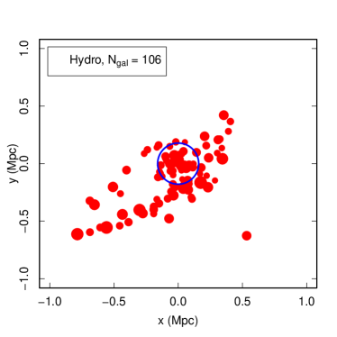
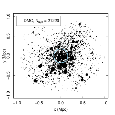
Figure 1: A comparison of the projected positions of dwarfs with total mass above $10^{7}\rm M_{\odot}$, as represented by filled circles, in the X-Y plane at z=0 within 1 Mpc from the central galaxy between the hydrodynamical (left) and the dark matter-only (right) simulations. The size of the circle is proportional to the halo mass, and the open circle in the center of the two plots indicates the virial radius of the simulated Milky Way at $\sim$ 240 kpc at z=0.

2.3.2 Tensor of Inertia method

This is a common method that has been used in literature (Pawlowski et al., 2015a) to determine the $a$, $b$, and $c$ axes of satellite distribution. In this method we find the moment of inertia of the dwarfs and diagonalize it to find the axes length ($a,b,c$) of the distribution. Let the position vector of a dwarf be given $\boldsymbol{r}_{i}=(x_{i},y_{i},z_{i})$. We calculate the tensor of inertia (TOI) matrix, weighted or unweighted and find the eigenvalues of that matrix. The TOI is a $3\times 3$ matrix which is given by

$${{\boldsymbol{I}}_{\rm covariance}} = \sum_{i=1}^{n}\left(\begin{array}[]{ccc}x_{i}^{2}&x_{i}y_{i}&x_{i}z_{i}\\ x_{i}y_{i}&y_{i}^{2}&y_{i}z_{i}\\ x_{i}z_{i}&y_{i}z_{i}&z_{i}^{2}\end{array}\right)\times w_{i}$$ (17)

This matrix has the same form as the covariance matrix discussed in PCA method. The term $w_{i}$ in the above equation refers to the weight assigned to the dwarfs in the system according to their distances. If $w_{i}=1$, then this reduces to the standard method where all dwarfs have the same weight irrespective of their distances. It has been argued that the far off dwarfs should carry less weight in determining the DoS plane as they have higher chances of being outliers (Bailin & Steinmetz, 2005). For completeness, we use two cases of reduced weights, $w_{i}=1/r_{i}$ and $w_{i}=1/r_{i}^{2}$ where $r_{i}=\sqrt{x_{i}^{2}+y_{i}^{2}+z_{i}^{2}}$. The three eigenvalues of this matrix ${\boldsymbol{I}}_{\rm TOI}$, gives the three axes of the dwarf distribution $a,b,c$ (largest eigenvalue is a and the smallest one is c). The anisotropy of the distribution is characterized by the ratio of the minor-to-major axis, $c/a$ (for isotropic distribution $c/a=1$). We will use the two methods, PCA and reduced TOI with weights 1, $1/r$ and $1/r^{2}$ for determining the $c/a$ ratios of our various samples in this paper. This will enable us to get a description of the dwarf distribution and examine the effects of the different methods discussed above.

3 Abundance and Spatial Distribution of Satellites at z=0

3.1 Effects of Baryons

Early $N$-body simulations of galaxies generally showed a rather isotropic distribution of dark matter subhalos surrounding the central galaxy (Kang et al., 2005), which has often been interpreted as a failure of $\Lambda$CDM cosmology (Kroupa et al., 2005; Metz et al., 2007; Kroupa et al., 2010; Pawlowski et al., 2012; Pawlowski & Kroupa, 2014). However, these simulations did not include the effect of baryons. Recent studies have shown that baryons play an important role in determining the properties of both subhalos and the main host (e.g. Zhu et al. 2016; Sawala et al. 2016), but little is known about how baryons affect DoS structure. In this study, we investigate the effect of baryons on the abundance and distribution of satellites of a MW-like galaxy, by comparing the baryonic simulation and its N-body counterpart (details in $\S\ref{sec:4methods}$).

Figure 1 shows the projected spatial distribution of all subhalos found within 1 Mpc of the MW center in both simulations. We find that there are many more subhalos ($\sim$ 21220) within the DMO simulation compared to the 106 luminous subhalos (dwarf galaxies) in the baryonic run, because most subhalos in the DMO simulation do not form stars and hence they are not identified as galaxies. In Zhu et al. (2016), we identified three major baryonic processes, namely adiabatic contraction, tidal disruption, and reionization, that significantly affect the density distribution of dark matter halos and their ability to retain gas, thus reducing the star formation activity in many low-mass halos. Moreover, the DMO dwarfs are distributed noticeably more isotropically compared to baryonic dwarfs, which have a clear anisotropic distribution as a result of reduced abundance of star-forming dwarfs and interactions with the central galaxy. Similar results of anisotropic distribution in baryonic simulations were also reported by Sawala et al. (2016). Even early studies (Zentner et al., 2005) showed that the N-body subhalos are not fully isotropic and the likely luminous subhalos (satellites) are even more anisotropically distributed. This figure demonstrates that baryonic processes have a profound impact on the abundances and spatial distribution of satellite galaxies around a central MW-type galaxy, and it illustrates the difference between N-body simulations and hydrodynamical simulations on the study of the DoS phenomenon (e.g. Pawlowski et al. 2015a; Sawala et al. 2016). Hereafter, we are going to focus on the detailed analysis of the dwarfs in the baryonic simulation.

Figure 2: Three-dimensional spatial distribution of satellites (black dots) within 1 Mpc from the central galaxy in the hydrodynamical simulation. The fitted plane of the satellites, using PCA method, is shown as the black plane and the disk plane of the simulated Milky Way is depicted as the brown plane.

In Figure 2 we fit the distribution of 106 dwarfs within 1 Mpc of the central galaxy with the PCA method (see § 2.3). Among the 106 dwarfs, about $77\%$ can be considered as residing in the same plane (dwarfs within the rms height), as indicated by the blue plane in the figure. The angle between our fitted DoS plane and the simulated MW disk (as indicated by the orange plane) is $\sim 75$ degrees, which is very close to the observed angle of $\sim 77.3$ degrees (Pawlowski et al., 2013).

However, as shown in Figure 3, the r.m.s. height of the DoS, fitted to 106 dwarfs within 1 Mpc, is $\sim$ 145 kpc, which is much larger than those reported from observations ($\sim 30$ kpc for 39 dwarfs within 365 kpc) which typically use a much smaller sample (Pawlowski et al. 2015b, Maji et al. 2017 (in prep)). We will address the effect of sample size on the DoS properties in the next section.

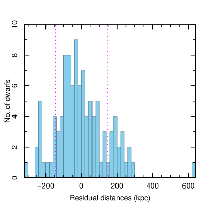
Figure 3: Distribution of the residual distances of the simulated satellites from the fitted DoS plane. The width between the two magenta dotted lines shows the root-mean-square height of the plane, $\sim 145$ kpc.

3.2 Effects of Sample Size and Plane Identification Method

In Maji et al. 2017 (in prep), we reanalyzed all dwarfs currently detected around the MW and grouped them in three subsets, as used by different groups in the literature: the 11 ’classical’ dwarfs (Kroupa et al., 2005), the 27 most massive nearby dwarfs and the complete sample of 39 dwarfs (Pawlowski et al., 2015b). We fit the three samples using both PCA and TOI methods (2.3) and found that both the isotropy (as indicated by $c/a$ ratio) and the thickness (characterized by the root-mean-square or r.m.s. height) of the DoS increase with sample size: the $c/a$ goes from $\sim 0.2$ for the 11 dwarfs to $\sim 0.26$ for the 39 dwarfs, and the r.m.s. height goes from $\sim 20$ kpc to $\sim 30$ kpc.

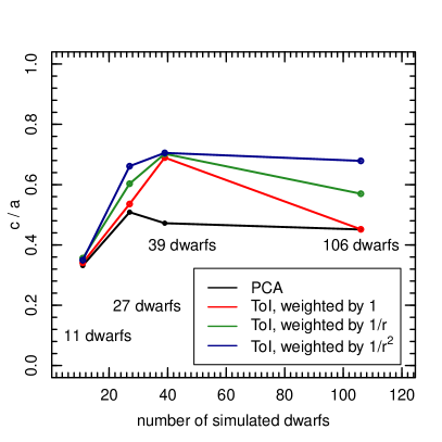
Figure 4: The “isotropy ” of the simulated satellite distribution, as indicated by $c/a$, as a function of the sample size. We have used four samples here with 11, 27, 39 and 106 dwarf galaxies respectively. The different colors denote the different plane fitting methods : Principal Component Analysis (black) and Tensor of Inertia with three types of weight functions, 1 (red), $1/r$ (green) and $1/r^{2}$ (blue).

To directly compare our simulated DoS with observations, we first calculate the farthest distance of the dwarfs from MW center for these three subsets and find them to be 257.4 kpc (Leo I), 257.4 kpc (Leo I) and 365 kpc (Eri II) for the sample of 11, 27 and 39 dwarfs respectively. Then we divide our simulated dwarfs into 4 subsets: 11 most massive (total mass) dwarfs within 257.4 kpc, 27 most massive dwarfs within 257.4 kpc, 39 most massive dwarfs within 365 kpc and for completeness, all 106 dwarfs within 1 Mpc. We apply the 4 methods discussed in § 2 and determine the $c/a$ ratio for these four samples, as shown in Figure  4. For the 11 dwarfs, the c/a ratio is $\sim 0.3$ in our simulation, close to the value of $\sim 0.2$ for the observations (Metz et al., 2007; Pawlowski et al., 2015b). However, with the full sample of 106 simulated dwarfs ($<1$ Mpc), the ratio increases to $\sim 0.44$ for PCA method, and it goes upto 0.68 for ToI method weighted by $1/r^{2}$. Similar range of $c/a$ was also reported by Sawala et al. (2016). This plot demonstrates that the DoS isotropy is subject to selection effect.

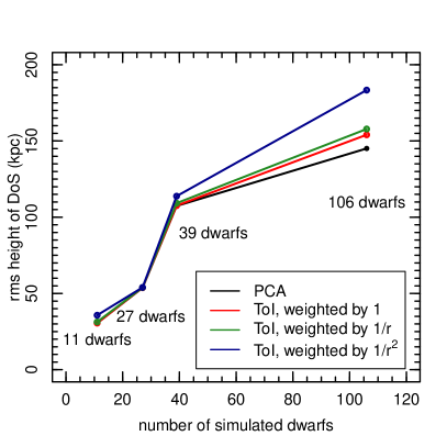
Figure 5: The root-mean-square (rms) height of the DoS plane fitted to a sample of simulated dwarfs as a function of the sample size. We have used the same four samples here with 11, 27, 39 and 106 dwarf galaxies respectively. The different colors denote same four plane fitting methods : Principal Component Analysis (black) and Tensor of Inertia with three types of weight functions, 1 (red), $1/r$ (green) and $1/r^{2}$ (blue).

Furthermore, in Figure 5 we show the r.m.s. heights of the simulated DoS plane for the four samples using four different methods and find that the DoS plane height increases with sample size. Using PCA method, the r.m.s. height for 11 dwarfs is $\sim 30$ kpc, and it rises to 120 kpc for 39 dwarfs and to 145 kpc when we include all dwarfs out to 1 Mpc. The thickness of the fitted DoS is even larger when ToI methods are used, as shown in the figure. For comparison, when Kroupa et al. (2005) took into account all known observed dwarfs upto 1 Mpc, the calculated r.m.s. DoS height was 159 kpc, close to our simulated height.

These results demonstrate that the DoS properties change significantly with the sample size of the satellites and the plane identification method. We have seen similar trends of changing DoS properties in observed satellites too as discussed in Maji et al. 2017, in prep. These considerations suggest that the properties of the highly flattened DoS of the MW derived from a small set of observed dwarfs (Ibata et al., 2013; Pawlowski et al., 2015a) may not be robust .

4 Kinematic Properties of Satellites at z=0

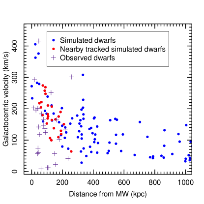
Figure 6: Comparison of galactocentric velocity between the simulated (blue points) and observed (purple crosses) dwarfs as a function of galactocentric distance. The observed data is taken from McConnachie (2012), and velocities are calculated with respect to the Galaxy. The red points are the 27 most massive dwarfs within 257.4 kpc of galactic center from the simulation.

Another claim of the DoS is that the satellites have coherent rotation in the same plane. It was suggested by Pawlowski et al. (2013) that, of the 11 “classical” dwarfs that have proper motion measurements, 7 to 9 are corotating on the DoS. However, in the analysis of Maji et al. 2017 (in prep.) we found that only 6 meet the criterion of corotation, and no firm coherent motion can be inferred. Moreover, these studies suffer from a very large uncertainties in the velocity measurements and a relatively small sample size. A larger sample size and precise measurements of 3-D velocity components of dwarfs from our simulation provide an advantageous study of the kinematic properties of the satellites.

Figure 6 shows the galactocentric velocity of the simulated dwarfs within 1 Mpc from the central galaxy, compared to Milky Way observations McConnachie (2012). Most of the observed dwarfs are located within 300 kpc from the MW, and they have a velocity range from $\sim 10$ to $\sim 400$ km/s. While the simulated ones have a similar velocity range, they have a higher median velocity ($\sim 150$ km/s compared to $\sim 100$ km/s from the observations).

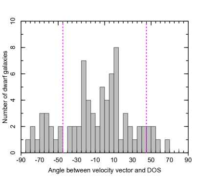
Figure 7: Distribution of the angle between velocity vector of simulate dwarfs and the DoS plane. The dwarfs whose velocity lies within -45 degree to +45 degree (magenta dotted lines) of the DoS are considered to be moving on the DoS.

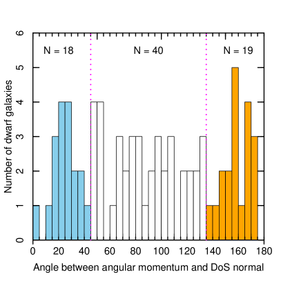
Figure 8: Distribution of angle between angular momentum of simulated dwarfs (residing in the DoS plane) and the DoS normal. There are 18 corotating (blue) and 19 counter-corotating (orange) dwarfs.

To investigate the kinematic coherence of the DoS, we first calculate the fraction of dwarfs moving in the DoS plane. We use a criterion to define a satellite as moving on the DoS when it total velocity vector falls from -45 to +45 degree of the DoS plane. As shown in Figure 7, 77 out of 106, or 73$\%$ of dwarfs within 1 Mpc, meet this criterion and are considered to be moving on the DoS. These dwarfs can be moving either mostly circularly (clockwise or counter clockwise) or mostly radially on the DoS.

Next, we calculate the fraction of dwarfs in the same circular motions (either corotation or counter-corotation) to determine whether or not the DoS is rotationally supported. We use a criterion to define a satellite as rotating on the DoS when its angular momentum vector falls from 0 to 45 degree of the DoS normal, or counter-corotating when the angle between the two is from 135 degree to 180 degree. As shown in Figure 8, out of the 77 satellites moving on the DoS, 18 are corotating and 19 are counter-corotating. If we consider all 106 satellites within 1 Mpc from the simulation, only $17\%$ are corotating and 18$\%$ are counter-corotating. These numbers strongly argue against any trend of corotation or counter-corotation, instead they show that the DoS is not rotationally supported.

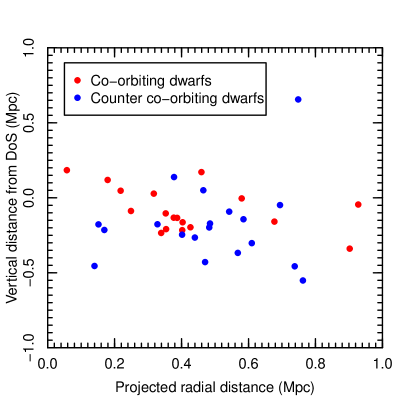
Figure 9: Vertical distance of the simulated dwarfs from the DoS vs their projected radial distance (i.e. the distance component lying on the DoS) from the center of the DoS (center-of-mass of the satellite galaxies). The red points show corotating dwarfs and blue points show counter-corotating dwarfs.

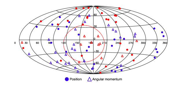
Figure 10: Positions and angular momenta of the observed (red symbols) satellites and simulated dwarfs (blue symbols) in Galactic coordinates are projected onto an Aitoff Hammer sphere. The filled circles and triangles represent the positions and angular momenta of the satellites, respectively. Satellites can be considered as corotating when their angular momenta are clustered in the same direction. For the observed momenta of 11 satellites, only 6 dwarfs near the center can be considered co-rotating; they are also within 45 degree of the DoS normal (depicted by red circle). Among the simulated momenta, no strong clustering of the majority of dwarfs are observed.

To further explore the coherent motion of the DoS, we examine the locations of the 18 corotating and 19 counter-corotating dwarfs, as shown in Figure 9. Not surprisingly, there is no correlation between spatial distribution and kinematic orientation of the satellites, the co-rotating or the counter-coorbiting dwarfs are not grouped in either radial or vertical direction, rather have a random distribution. This can be further demonstrated in the position – angular momentum distribution of the satellites. In Figure 10, we compare the Aitoff-Hammer projection of position and angular momentum of the 27 most massive satellites within the virial radius from the simulation with 27 observed dwarfs of the MW (though only 11 have angular momentum data). Although 6 observed dwarfs (Draco, Umi, SMC, Fornax, Leo II and LMC) may appear to be clustering in the angular momentum distribution (within 45 degree of 180 degree longitude and 0 degree latitude), spatially they are located far apart in different longitude–latitude planes. Similarly, no strong angular momentum clustering, or position – angular momentum correlation, is seen in the simulation. These results suggest that the DoS does not have coherent rotation.

Similar conclusions have been reported by other studies on DoS. Cautun et al. (2015b) and Phillips et al. (2015) found that the apparent excess of corotating dwarfs around SDSS galaxies, as claimed by Ibata et al. (2014a), is highly sensitive to sample selection criterion and sample size, and it is consistent with the noise expected from an under-sampled data. These findings suggest that the DoS in general is not a kinematically coherent structure.

5 Evolution of Satellites

5.1 Evolution of Spatial Distribution

In order to directly probe the origin of the DoS or the anisotropic distribution of the satellite system, it is essential to observe them at high redshift. However, due to the low luminosity of the satellite galaxies, it is extremely difficult to observe them in the distant universe. Other than the satellites in our Local Group, we have observations of possible DoS around SDSS galaxies only up to $z=0.05$ (Ibata et al., 2014a). However these claims have been largely refuted (Cautun et al., 2015a; Phillips et al., 2015).

In the simulations we can track the satellite systems to very high redshift. In Fig 11, we follow the 3D distribution of the satellites from redshift $z=10$ to the present day, with the 27 most massive ones highlighted in order to understand those observed in the MW. At redshift $z=10$, the overall distribution of the galaxies is almost isotropic. After $z=6$, the number of dwarfs decreases significantly, mostly due the disruption of low-mass halos after reionization (Zhu et al., 2016). After $z=4$, the galaxies become more strongly clustered along the filaments, as expected from the standard hierarchical structure formation model (Springel et al., 2005; Vogelsberger et al., 2014), and the distribution becomes more anisotropic with time. As it approaches to $z=0$, the distribution of the satellite system becomes strongly anisotropic.

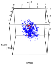
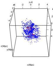
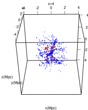
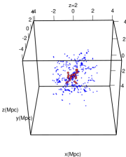
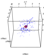
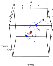
Figure 11: Spatial distribution of all dwarfs (blue points) within 3 Mpc of Milky Way (comoving scale) at different redshifts, namely $z=10,6,4,1$ and $0$. The red points are the 27 most massive satellites within 257.4 kpc of the galactic center at $z=0$ which were tracked at higher redshifts. The overall distribution of the dwarfs is nearly isotropic at high redshifts but it gradually evolves to be anisotropic with time.

To quantify the change over time, we fit the satellite system at different redshifts with 4 different plane identification methods (discussed in section 2.3). The resulting evolution of the $c/a$ ratio is shown in Figure 12. We find that all methods give a consistent high $c/a$ ratio at high redshift, which generally decreases with time. This change is most prominent with both PCA and the unweighted ToI method, where the “isotropy” index starts at $c/a\sim 0.7$ at $z=10$ but drops to $c/a\sim 0.44$ at $z=0$. These results suggest that the DoS structure is a result of the galaxy formation and evolution process and part of the large-scale filamentary structure.

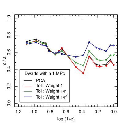
Figure 12: Evolution of the isotropy ratio ($c/a$) of the simulated satellite distribution within 1 Mpc. Different colors the figure denote different plane fitting methods : Principal Component Analysis (black) and Tensor of Inertia with three types of weight functions, 1 (red), $1/r$ (green) and $1/r^{2}$ (blue).

To investigate the large scale dynamics of the dwarfs, we show their 3D velocity vectors in Figure 13. Around the galactic center, the velocity vectors appear to be random and do not show any preferential rotation, as we have also seen in previous sections. This is the result of different accretion history and trajectory of individual dwarfs into the main galaxy as shown in Zhu et al. (2016). However, at large distances the dwarfs are moving toward a narrow elongated direction, which suggests that they are part of the large scale filamentary structure.

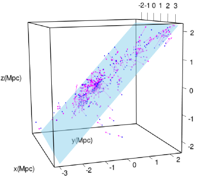
Figure 13: Three dimensional plot of simulated dwarf positions (blue points), within 3 Mpc of the galactic center, along with the DoS plane (blue plane) fitted by PCA method. The 3D velocities of these dwarf galaxies are represented by the magenta arrows and the length of these arrows is proportional to the velocity magnitude.

5.2 Evolution of the Kinematics

The evolution of the kinematic properties of the dwarfs is shown in Figure 14, in which we track dwarf subsets with different kinematical properties: dwarfs moving on the DoS and rotating ones which include corotating and counter-corotating. We find that over the redshift range from $z=2$ to $z=0$, the different fractions remain nearly the same. Around $80\%$ of these galaxies are primarily moving on DoS (as opposed to normal to DoS) and around $45\%$ of them are rotating on the DoS, the rest is moving radially.

Interestingly, the fractions of corotating and counter-corotating dwarfs are comparable at around $20\%$ throughout the time. This reaffirms our conclusion that the DoS has no coherent rotation and it is not rotationally supported.

Figure 14: Evolution of the fraction of dwarfs (within 1 Mpc of galactic center) with different kinematical properties : the fraction of dwarfs moving on the DoS plane (black), the fraction of dwarfs co-rotating in DoS (red), the fraction of dwarfs counter co-rotating in DoS (blue), and the total fraction of dwarfs rotating (corotating and counter-corotating) in DoS (magenta).

6 Discussions

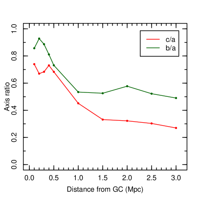
Figure 15: The $c/a$ ratio (red) and the $b/a$ ratio (green) of the dwarf distribution as a function of the maximum distance of the dwarfs from galactic center. For each distance, we take all dwarfs within that radius and calculate these two ratios using PCA method.

In order to investigate how the DoS structure changes with the distance from the central galaxy, we plot the two different axis ratios ($c/a$ and $b/a$) of the dwarf distribution at different radii from the galactic center in Figure 15. We find that both ratios decreases with increasing distance, by 3 Mpc, $c/a\sim 0.25$ and $b/a\sim 0.5$, which may resemble the large-scale filamentary structure. However, we note that when we include all the dwarfs (not just the most massive ones as in the previous sections), the distribution becomes more isotropic close to the galactic center compared to the distribution of only massive dwarfs.

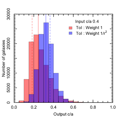
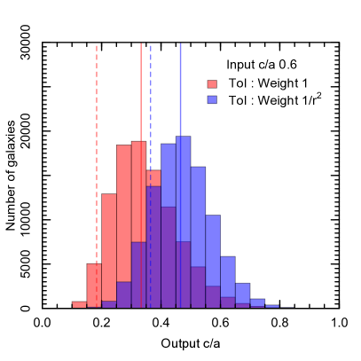
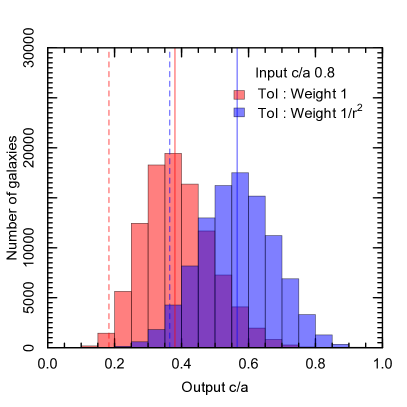
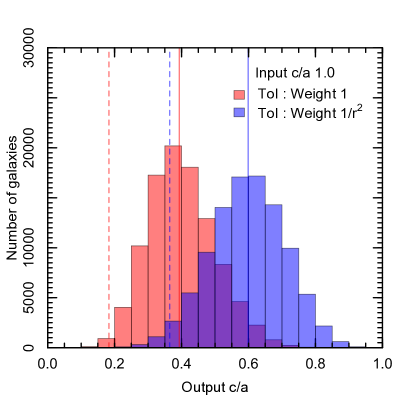
Figure 16: Distribution of output galaxy c/a for different input values ($c/a=0.4$ top left panel, 0.6 in top right panel, 0.8 in bottom left panel and 1.0 in bottom right panel) in a Monte Carlo simulation with 100,000 galaxies. The c/a ratio is calculated by two methods: weighted by 1 (red), and weighted by $1/r^{2}$ (blue). The violet region shows the overlap between the distributions with two methods. The dashed vertical lines in red and blue shows the observed c/a value calculated with 11 MW satellites with these two methods respectively. The median $c/a$ values for the systems are shown with vertical red (weight 1) and blue (weight $1/r^{2}$) solid lines.

Furthermore, we note that the $c/a$ ratio may not adequately represent the underlying distribution of the system. To demonstrate this, we take the observed positions of the 11 classical dwarfs and perform four tests on them. In the first test, we distribute the 11 dwarfs in their observed distances but placing them in a way such that their input $c/a=0.4$. Now we perform a Monte Carlo simulation for 100,000 realizations of this system and calculate the $c/a$ ratio of each realization using two weighted methods (weights 1, and $1/r^{2}$ respectively, details in §2.3.2). We plot the distribution of the output $c/a$ ratio of these galaxies in Figure 16 (top left panel) and find that although the input $c/a=0.4$, about $\sim 20\%$ of the systems have an output $c/a\lesssim 0.18$, the observed anisotropy ratio for the observed 11 galaxies (with weight 1 method). We repeat this test with three other input $c/a$, 0.6, 0.8 and 1.0 respectively and find that for each of them there is non-negligible probability that the system has a lower output $c/a$ than the input value. We also notice that the method used to determine the $c/a$ ratio also influences the output, for all samples, the weighted by $1/r^{2}$ method produces higher $c/a$ than the unweighted method. This shows that very small samples, i.e. 11 dwarfs, may artificially indicate a higher anisotropy and they may not contain the full information of the underlying distribution.

Finally we stress that our results are subject to the limitations of our study, as we have only analyzed one particular realization of a MW-sized galaxy. In future projects we plan to pursue a more systematic study by extending our simulated galaxy sample.

7 Summary

We have investigated the spatial distribution and kinematic properties of satellites of a MW-sized galaxy by comparing a high resolution hydrodynamical cosmological simulation with its DM only counterpart. Our main results are summarized as follows:

• Baryons play a significant role in determining the abundance and distribution of the satellite system of a galaxy. Within 1 Mpc from the central galaxy, only 106 dwarf galaxies containing stars are found at the present day in the hydrodynamic simulation and they show an anisotropic distribution, in sharp contrast to 21,220 subhalos in the N-body simulation, which are distributed isotropically;

• The DoS in our simulation is not rotationally supported and there is no coherent motion of the satellites, as the fraction of corotating and counter-corotating satellites are comparable and around $19\%$ across cosmic time.

• The distribution of the (baryonic) satellite galaxy system evolves significantly with time. It is highly isotropic at high redshifts but it becomes more anisotropic as redshift approaches to $z=0$, and this anisotropic distribution is part of the filamentary structure in the hierarchical structure formation scenario.

• The properties of the DoS strongly depend on the sample size and the plane identification methods. When only the 11 most massive dwarfs similar to those “classical” Milky Way satellites are selected, the DoS becomes more flattened as observed. However, when the sample size increases the DoS becomes thicker. This is consistent with the observational pattern that height and the flatness ratio of the DoS increase with sample size, as shown in Maji et. al. 2017 (in prep.).

Our results suggest that the highly-flattened, coherently-rotating DoS claimed in the MW and other galaxies may be a selection effect due to a small sample size, and that different subhalo distributions that we see in our hydrodynamical and N-body simulations are shaped by baryons. Baryonic processes such as adiabatic contraction, reionization, and tidal destruction of galaxies can have significant effects on the abundance, star formation, infall time and trajectories of the satellites which can in turn affect their final distribution. Therefore, effects of baryons should be taken into account in the study of the distribution and evolution of the satellite system of a galaxy.

References

- Agustsson & Brainerd (2010) Agustsson, I., & Brainerd, T. G. 2010, ApJ, 709, 1321
- Azzaro et al. (2007) Azzaro, M., Patiri, S. G., Prada, F., & Zentner, A. R. 2007, MNRAS, 376, L43
- Bahl & Baumgardt (2014) Bahl, H., & Baumgardt, H. 2014, MNRAS, 438, 2916
- Bailin et al. (2008) Bailin, J., Power, C., Norberg, P., Zaritsky, D., & Gibson, B. K. 2008, MNRAS, 390, 1133
- Bailin & Steinmetz (2005) Bailin, J., & Steinmetz, M. 2005, ApJ, 627, 647
- Boylan-Kolchin et al. (2009) Boylan-Kolchin, M., Springel, V., White, S. D. M., Jenkins, A., & Lemson, G. 2009, MNRAS, 398, 1150
- Brainerd (2005) Brainerd, T. G. 2005, ApJ, 628, L101
- Buck et al. (2016) Buck, T., Dutton, A. A., & Macciò, A. V. 2016, MNRAS
- Cautun et al. (2015a) Cautun, M., Bose, S., Frenk, C. S., Guo, Q., Han, J., Hellwing, W. A., Sawala, T., & Wang, W. 2015a, MNRAS, 452, 3838
- Cautun et al. (2015b) Cautun, M., Wang, W., Frenk, C. S., & Sawala, T. 2015b, MNRAS, 449, 2576
- Conn et al. (2013) Conn, A. R., Lewis, G. F., Ibata, R. A., Parker, Q. A., Zucker, D. B., McConnachie, A. W., Martin, N. F., Valls-Gabaud, D., Tanvir, N., Irwin, M. J., Ferguson, A. M. N., & Chapman, S. C. 2013, ApJ, 766, 120
- Davis et al. (1985) Davis, M., Efstathiou, G., Frenk, C. S., & White, S. D. M. 1985, ApJ, 292, 371
- Gill et al. (2004) Gill, S. P. D., Knebe, A., & Gibson, B. K. 2004, MNRAS, 351, 399
- Hellwing et al. (2016) Hellwing, W. A., Frenk, C. S., Cautun, M., Bose, S., Helly, J., Jenkins, A., Sawala, T., & Cytowski, M. 2016, MNRAS, 457, 3492
- Helmi (2008) Helmi, A. 2008, A&A Rev., 15, 145
- Holmberg (1969) Holmberg, E. 1969, Arkiv for Astronomi, 5, 305
- Ibata et al. (2014a) Ibata, N. G., Ibata, R. A., Famaey, B., & Lewis, G. F. 2014a, Nature, 511, 563
- Ibata et al. (2014b) Ibata, R. A., Ibata, N. G., Lewis, G. F., Martin, N. F., Conn, A., Elahi, P., Arias, V., & Fernando, N. 2014b, ApJ, 784, L6
- Ibata et al. (2013) Ibata, R. A., Lewis, G. F., Conn, A. R., Irwin, M. J., McConnachie, A. W., Chapman, S. C., Collins, M. L., Fardal, M., Ferguson, A. M. N., Ibata, N. G., Mackey, A. D., Martin, N. F., Navarro, J., Rich, R. M., Valls-Gabaud, D., & Widrow, L. M. 2013, Nature, 493, 62
- Kang et al. (2005) Kang, X., Mao, S., Gao, L., & Jing, Y. P. 2005, A&A, 437, 383
- Knollmann & Knebe (2009) Knollmann, S. R., & Knebe, A. 2009, ApJS, 182, 608
- Koch & Grebel (2006) Koch, A., & Grebel, E. K. 2006, AJ, 131, 1405
- Koposov et al. (2015) Koposov, S. E., Belokurov, V., Torrealba, G., & Evans, N. W. 2015, ApJ, 805, 130
- Kroupa et al. (2010) Kroupa, P., Famaey, B., de Boer, K. S., Dabringhausen, J., Pawlowski, M. S., Boily, C. M., Jerjen, H., Forbes, D., Hensler, G., & Metz, M. 2010, A&A, 523, A32
- Kroupa et al. (2005) Kroupa, P., Theis, C., & Boily, C. M. 2005, A&A, 431, 517
- Kunkel & Demers (1976) Kunkel, W. E., & Demers, S. 1976, in Royal Greenwich Observatory Bulletins, Vol. 182, The Galaxy and the Local Group, ed. R. J. Dickens, J. E. Perry, F. G. Smith, & I. R. King, 241
- Lynden-Bell (1976) Lynden-Bell, D. 1976, MNRAS, 174, 695
- Marinacci et al. (2014) Marinacci, F., Pakmor, R., & Springel, V. 2014, MNRAS, 437, 1750
- McConnachie (2012) McConnachie, A. W. 2012, AJ, 144, 4
- McConnachie et al. (2009) McConnachie, A. W., Irwin, M. J., Ibata, R. A., Dubinski, J., Widrow, L. M., Martin, N. F., Côté, P., Dotter, A. L., Navarro, J. F., Ferguson, A. M. N., Puzia, T. H., Lewis, G. F., Babul, A., Barmby, P., Bienaymé, O., Chapman, S. C., Cockcroft, R., Collins, M. L. M., Fardal, M. A., Harris, W. E., Huxor, A., Mackey, A. D., Peñarrubia, J., Rich, R. M., Richer, H. B., Siebert, A., Tanvir, N., Valls-Gabaud, D., & Venn, K. A. 2009, Nature, 461, 66
- Metz et al. (2007) Metz, M., Kroupa, P., & Jerjen, H. 2007, MNRAS, 374, 1125
- Pawlowski et al. (2015a) Pawlowski, M. S., Famaey, B., Merritt, D., & Kroupa, P. 2015a, ApJ, 815, 19
- Pawlowski & Kroupa (2014) Pawlowski, M. S., & Kroupa, P. 2014, ApJ, 790, 74
- Pawlowski et al. (2012) Pawlowski, M. S., Kroupa, P., Angus, G., de Boer, K. S., Famaey, B., & Hensler, G. 2012, MNRAS, 424, 80
- Pawlowski et al. (2013) Pawlowski, M. S., Kroupa, P., & Jerjen, H. 2013, MNRAS, 435, 1928
- Pawlowski et al. (2015b) Pawlowski, M. S., McGaugh, S. S., & Jerjen, H. 2015b, MNRAS, 453, 1047
- Phillips et al. (2015) Phillips, J. I., Cooper, M. C., Bullock, J. S., & Boylan-Kolchin, M. 2015, MNRAS, 453, 3839
- Sales & Lambas (2004) Sales, L., & Lambas, D. G. 2004, MNRAS, 348, 1236
- Sawala et al. (2016) Sawala, T., Frenk, C. S., Fattahi, A., Navarro, J. F., Bower, R. G., Crain, R. A., Dalla Vecchia, C., Furlong, M., Helly, J. C., Jenkins, A., Oman, K. A., Schaller, M., Schaye, J., Theuns, T., Trayford, J., & White, S. D. M. 2016, MNRAS, 457, 1931
- Springel (2010) Springel, V. 2010, MNRAS, 401, 791
- Springel et al. (2005) Springel, V., White, S. D. M., Jenkins, A., Frenk, C. S., Yoshida, N., Gao, L., Navarro, J., Thacker, R., Croton, D., Helly, J., Peacock, J. A., Cole, S., Thomas, P., Couchman, H., Evrard, A., Colberg, J., & Pearce, F. 2005, Nature, 435, 629
- Vogelsberger et al. (2014) Vogelsberger, M., Genel, S., Springel, V., Torrey, P., Sijacki, D., Xu, D., Snyder, G., Bird, S., Nelson, D., & Hernquist, L. 2014, Nature, 509, 177
- Willman (2010) Willman, B. 2010, Advances in Astronomy, 2010, 285454
- Zaritsky et al. (1997) Zaritsky, D., Smith, R., Frenk, C. S., & White, S. D. M. 1997, ApJ, 478, L53
- Zentner et al. (2005) Zentner, A. R., Kravtsov, A. V., Gnedin, O. Y., & Klypin, A. A. 2005, ApJ, 629, 219
- Zhu et al. (2015) Zhu, Q., Hernquist, L., & Li, Y. 2015, ApJ, 800, 6
- Zhu et al. (2016) Zhu, Q., Marinacci, F., Maji, M., Li, Y., Springel, V., & Hernquist, L. 2016, MNRAS, 458, 1559