Effect of long-range interaction on graphene edge magnetism

Abstract

It has been proposed that interactions lead to ferromagnetism on a zigzag edge of a graphene sheet. While not yet directly studied experimentally, dramatically improving techniques for making and studying clean zigzag edges may soon make this possible. So far, most theoretical investigations of this claim have been based on mean field theories or more exact calculations using the Hubbard model. But long-range Coulomb interactions are unscreened in graphene so it is important to consider their effects. We study rather general non-local interactions, including of Coulomb $1/r$ form, using the technique of projection to a strongly interacting edge Hamiltonian, valid at first order in the interactions. The ground states as well as electron/hole and exciton excitations are studied in this model. Our results indicate that ferromagnetism survives with unscreened Coulomb interactions.

I Introduction

Non-interacting graphene nanoribbons with zigzag edges are famous for hosting a nearly flat band of edge states.Fujita et al. (1996); Wakabayashi et al. (2010) In the presence of electron-electron interaction, the existence of edge magnetic orderYazyev (2010) has been predicted by a multitude of theoretical work using both analyticalFujita et al. (1996); Yamashiro et al. (2003); Jung et al. (2009); *PhysRevB.79.235433; Rhim and Moon (2009); Schmidt and Loss (2010); Jung (2011); Culchac et al. (2011); Schmidt (2012); Karimi and Affleck (2012) and numericalLuitz et al. (2011); Schmidt et al. (2013); Wunsch et al. (2008); Golor et al. (2013a, b, 2014); *PhysRevB.87.245431; Hagymási and Legeza (2016); Son et al. (2006); Pisani et al. (2007); Huang et al. (2013) techniques. The consensus emerging from these work is that edge states localized at the same edge are coupled ferromagnetically to form superspins, which then couple antiferromagnetically between edges. In addition to ground state properties, low-energy magnetic excitations in graphene nanoribbons have also attracted much theoretical attention.Wakabayashi et al. (1998); Yazyev and Katsnelson (2008); Rhim and Moon (2009); Culchac et al. (2011) A relatively large spin correlation length up to the order of micrometers has been found for a single zigzag edge; this is attributed to the large spin stiffness in this system, and boosts confidence in potential spintronics applications of graphene edge magnetism.Zhang et al. (2010) Although conclusive experimental evidence for edge magnetism is still lacking due to limited control over edge orientation, there has been significant progress in recent years towards the synthesis and characterization of zigzag edges.Magda et al. (2014); Ruffieux et al. (2015); Makarova et al. (2015)

A large number of theoretical studies on graphene edge magnetism represent the interaction by an on-site Hubbard term for simplicity. For the Hubbard model on a honeycomb lattice, arguments in support of edge magnetismKarimi and Affleck (2012) can be constructed based on Lieb’s theorem.Lieb (1989) The Coulomb interaction in pristine graphene on a non-metallic substrate is, nevertheless, poorly screened due to a vanishing density of states at the Dirac points.DiVincenzo and Mele (1984); Kotov et al. (2012) The influence of non-local components of the interaction has been investigated both in bulk grapheneWu and Tremblay (2014); Herbut (2006); Honerkamp (2008); Schüler et al. (2013) and in restricted geometries.Yamashiro et al. (2003); Jung (2011); Chacko et al. (2014); Zhu and Wang (2006); Wunsch et al. (2008) (By “non-local” we mean having a longer range than on-site.) However, many studies on graphene nanoribbons with non-local interactions have adopted a mean-field treatment, neglecting fluctuations whose role is especially important in low dimensions.Mermin and Wagner (1966) Exact diagonalization has been employed in other studies; despite the light it sheds on the nature of the ground states, correlations in manageably small systems are usually enhanced compared to the thermodynamic limit.

In the present work, we study the effect of long-range interactions on graphene edge ferromagnetism, in the limit of weak interactions but beyond the mean-field level. Focusing on a semi-infinite graphene sheet with a single zigzag edge, we find the effective Hamiltonian by projecting the interaction into the Hilbert space of edge states; we then propose a sufficient condition for the maximum spin ferromagnetic multiplet to be the half-filling ground states. Using exact diagonalization, we discuss the possible ground states for interactions in violation of this condition. The long-range Coulomb interaction is shown to satisfy the sufficient condition upon extrapolation to the limit of infinite long distance cutoff. We also examine the simplest low-energy excitations of the ferromagnetic ground states on a single edge. For short-range interactions, single-particle excitations and single-hole excitations have linear spectra $\propto v\delta k$ where $\left|\delta k\right|\ll 1$ is the distance from either Dirac point, with a slope $v$ controlled by the interaction strength. Spin-1 excitons have a small-momentum dispersion that is proportional to $vQ^{2}\ln Q$. For the long-range Coulomb interaction, $v\rightarrow\infty$, and the dispersion of single-particle or single-hole excitations near the Dirac points scales as $\delta k\ln\delta k$. Finally, for both short-range and Coulomb interactions, a sufficiently large particle-hole symmetry breaking term in the Hamiltonian can destabilize the ferromagnetic ground state.

II Model

We study a semi-infinite graphene sheet on the $xy$ plane, modeled by a honeycomb lattice which is terminated by an infinite zigzag edge (see Fig. 1). All carbon atoms reside in the half plane $y\geq 0$, and the outermost atoms on the zigzag edge (which belong to the $A$ hexagonal sublattice) lie on the $x$ axis. In units of the Bravais lattice constant $a=2.46$Å, it is convenient to represent the position of carbon atoms by $\vec{r}_{\left(m,n\right)}=\left(m/2\right)\hat{x}+\left(\sqrt{3}n/2\right)\hat{y}$ where $n\geq 0$. While $m$ is always an integer, note that $n$ is an integer only on the $A$ sublattice: for $A$ atoms $n$ and $m$ are both even or both odd, while for $B$ atoms $n+2/3$ and $m$ are both even or both odd.

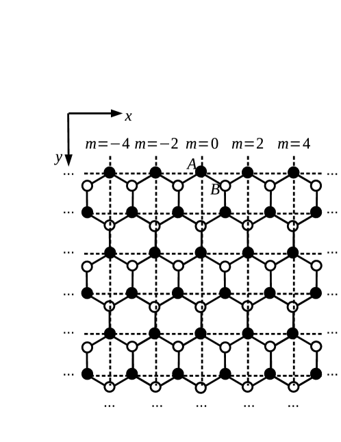
Figure 1: Sketch of a semi-infinite graphene sheet with a zigzag edge.

The zero modes associated with the zigzag edge are given byFujita et al. (1996); Wakabayashi et al. (2010)

$$e_{k}^{{\dagger}}=\frac{1}{\sqrt{2\pi}}\sum_{n\geq 0,m}e^{ik\frac{m}{2}}g_{n}\left(k\right)c_{m,n,A}^{{\dagger}}\text{,}$$ (1)

where $k$ is the crystal momentum along the edge direction,

$$g_{n}\left(k\right)\equiv\theta\left(k-\frac{2\pi}{3}\right)\theta\left(\frac{4\pi}{3}-k\right)\sqrt{1-4\cos^{2}\frac{k}{2}}\left(-2\cos\frac{k}{2}\right)^{n}$$ (2)

describes the decay of the wave function into the bulk, and the $c$ operators obey the usual anticommutation relations $\left\{c_{m,n,A},c_{m^{\prime},n^{\prime},A}^{{\dagger}}\right\}=\left\{c_{m,n,B},c_{m^{\prime},n^{\prime},B}^{{\dagger}}\right\}=\delta_{mm^{\prime}}\delta_{nn^{\prime}}$, $\left\{c_{m,n,A},c_{m^{\prime},n^{\prime},B}^{{\dagger}}\right\}=0$. (We have temporarily suppressed the spin index.) These edge states exist only for $2\pi/3<k<4\pi/3$, i.e. in $1/3$ of the 1D Brillouin zone $0\leq k<2\pi$. The wave function is non-zero only on the $A$ sublattice, and is localized near the zigzag edge. The localization length $\xi_{k}=-\left[\ln\left|2\cos\left(k/2\right)\right|\right]^{-1}$ vanishes at $k=\pi$, and diverges near the Dirac points $k=2\pi/3$ and $k=4\pi/3$.

In addition to the edge states, we also have bulk states which are labeled by $k$, $k_{y}$ and $s$:

$$b_{k,k_{y},s}^{{\dagger}} = \frac{1}{2\pi}\frac{1}{\sqrt{2}}\left\{\sum_{n\geq 0,m}e^{ik\frac{m}{2}}\left[2i\sin nk_{y}+\left(2\cos\frac{k}{2}\right)2i\sin\left(n+1\right)k_{y}\right]\right.$$ (3)

$$\left.\times\frac{t}{E_{s}\left(k,k_{y}\right)}c_{m,n,A}^{{\dagger}}-\sum_{n\geq\frac{1}{3},m}e^{ik\frac{m}{2}}\left[2i\sin\left(n+\frac{2}{3}\right)k_{y}\right]c_{m,n,B}^{{\dagger}}\right\}\text{.}$$

Here the bulk dispersion relation is

$$E_{s}\left(k,k_{y}\right)=st\sqrt{\left(2\cos\frac{k}{2}\right)^{2}+1+2\left(2\cos\frac{k}{2}\right)\cos k_{y}}$$ (4)

with nearest neighbor hopping strength $t$; $k_{y}$ is the crystal momentum perpendicular to the edge, $0\leq k_{y}\leq\pi$, and $s=\pm$ is a subband index. Near the Dirac points, where $\left(k,k_{y}\right)=\left(2\pi/3,\pi\right)+\left(\delta k,\delta k_{y}\right)$ or $\left(k,k_{y}\right)=\left(4\pi/3,0\right)+\left(\delta k,\delta k_{y}\right)$, $E_{s}\left(k,k_{y}\right)$ takes a Lorentz invariant form $E_{s}\left(k,k_{y}\right)=st\sqrt{\left(\delta k_{y}\right)^{2}+\left(3/4\right)\left(\delta k\right)^{2}}$. In this non-interacting model, at zero temperature and half-filling, the $s=-$ subband is completely filled and the $s=+$ subband is completely empty. While the edge states are half-filled, for the semi-infinite sheet we cannot ascertain which half is filled at this point, unless other ingredients–such as next-nearest-neighbor hopping, edge potential and electron-electron interaction–are present.

We now introduce a weak repulsive electron-electron interaction. The following extended Hubbard model manifestly respects $SU\left(2\right)$ spin symmetry, and also particle-hole symmetry at half-filling:

$$H_{int}=\frac{1}{2}\sum_{n,m}\sum_{\delta_{m},\delta_{n}}U_{\left(\delta_{m},\delta_{n}\right)}\left(\sum_{\sigma=\pm}c_{m,n,\sigma}^{{\dagger}}c_{m,n,\sigma}-1\right)\left(\sum_{\sigma^{\prime}=\pm}c_{m+\delta_{m},n+\delta_{n},\sigma^{\prime}}c_{m+\delta_{m},n+\delta_{n},\sigma^{\prime}}-1\right)\text{.}$$ (5)

$\left(\delta_{m},\delta_{n}\right)$ runs over all vectors $\vec{\delta}=\left(\delta_{m}/2\right)\hat{x}+\left(\sqrt{3}\delta_{n}/2\right)\hat{y}$ pointing from one lattice site to another; for instance, $U_{\left(0,0\right)}$ stands for the strength of the on-site Hubbard interaction, $U_{\left(0,2/3\right)}$ is the interaction between nearest neighbor sites (belonging to different sublattices) in the $y$ direction, $U_{\left(1,1/3\right)}$ is the interaction between nearest neighbor sites at $\pi/6$ angle with the $x$ direction, and $U_{\left(2,0\right)}$ is the interaction between next nearest neighbors (belonging to the same sublattice) in the $x$ direction. The sum over $n$ and $\delta_{n}$ is such that both $n\geq 0$ and $n+\delta_{n}\geq 0$. To lighten notations, we have suppressed the sublattice indices $A$ and $B$ in this expression, because they are uniquely determined by the position indices $\left(m,n\right)$ and $\left(m+\delta_{m},n+\delta_{n}\right)$.

In general $U_{\left(\delta_{m},\delta_{n}\right)}=U_{\left(-\delta_{m},-\delta_{n}\right)}$, but apart from this constraint $U$ can be an arbitrary function of $\delta_{m}$ and $\delta_{n}$. Nevertheless we further assume that $U$ obeys parity symmetry, $U_{\left(\delta_{m},\delta_{n}\right)}=U_{\left(-\delta_{m},\delta_{n}\right)}$. For the Hubbard model, $U_{\left(\delta_{m},\delta_{n}\right)}$ vanishes unless $\delta_{m}=\delta_{n}=0$. On the other hand, for the unscreened Coulomb interaction, $U_{\left(\delta_{m},\delta_{n}\right)}$ is inversely proportional to distance at large distances,Egger and Gogolin (1997); Zarea and Sandler (2007); *PhysRevLett.101.196804; Jung (2011)

$$U_{\left(\delta_{m},\delta_{n}\right)}=U_{0}\frac{d}{\sqrt{d^{2}+\left|\vec{\delta}\right|^{2}}}\text{,}$$ (6)

where $U_{0}$ is the on-site interaction, and the half-nearest-neighbor distance $d=1/\left(2\sqrt{3}\right)$ accounts for the finite spread of the carbon $\pi$ orbitals.

Assuming $U_{\left(\delta_{m},\delta_{n}\right)}\ll t$, we expect that the low-energy degrees of freedom are composed of the edge states $e_{k}$ with $2\pi/3<k<4\pi/3$, and the bulk states in the vicinity of the two Dirac points.Wunsch et al. (2008); Schmidt et al. (2013) As a first approximation at $O\left(U\right)$, we neglect the dynamics of the bulk states completely; they are assumed to be half-filled and not spin-polarized as in the non-interacting case.Schmidt and Loss (2010); Karimi and Affleck (2012) This approximation allows the projection of the interaction onto the Hilbert space of the edge states. More concretely, we invert Eqs. (1) and (3) to express the $c$ operators in terms of $e$ and $b$, then take the expectation values for pairs of $b$ operators using

$$\left\langle b_{k,k_{y},-,\sigma}^{{\dagger}}b_{k^{\prime},k_{y}^{\prime},-,\sigma^{\prime}}\right\rangle=\left\langle b_{k,k_{y},+,\sigma}b_{k^{\prime},k_{y}^{\prime},+,\sigma^{\prime}}^{{\dagger}}\right\rangle=\delta_{\sigma\sigma^{\prime}}\delta\left(k-k^{\prime}\right)\delta\left(k_{y}-k_{y}^{\prime}\right)\text{.}$$ (7)

After some algebra, we find

$$H_{\text{int}}=\frac{1}{2}\sum_{n}\sum_{\delta_{m},\delta_{n}}U_{\left(\delta_{m},\delta_{n}\right)}\int_{-\frac{2\pi}{3}}^{\frac{2\pi}{3}}\frac{dq}{2\pi}e^{iq\frac{\delta_{m}}{2}}O_{n+\delta_{n}}^{{\dagger}}\left(q\right)O_{n}\left(q\right)\text{,}$$ (8)

where the sum over $\left(\delta_{m},\delta_{n}\right)$ is now limited to vectors on one of the sublattices; recalling that edge states only exist on the $A$ sublattice, $\delta_{m}$ and $\delta_{n}$ are now both even or both odd. Again $n\geq 0$ and $n+\delta_{n}\geq 0$. $O_{n}\left(q\right)$ is bilinear in $e$,

$$O_{n}\left(q\right)\equiv\int dkg_{n}\left(k+q\right)g_{n}\left(k\right)\left[\sum_{\sigma=\pm}e_{k+q,\sigma}^{{\dagger}}e_{k,\sigma}-\delta\left(q\right)\right]\text{.}$$ (9)

$q$ measures the momentum difference between two edge states, so the operator $O_{n}\left(q\right)$ is nontrivial only when $\left|q\right|<2\pi/3$. Note that $O_{n}\left(q\right)$ annihilates all members of the fully polarized ferromagnetic multiplet at half-filling for any $n$ and $q$, which means the ferromagnetic multiplet states are always eigenstates of $H_{\text{int}}$ with zero energy.

Due to the constraint on the $\left(\delta_{m},\delta_{n}\right)$ summation, many terms in the interaction (most notably the nearest-neighbor interaction) do not enter the projected effective Hamiltonian in the edge state subspace, Eq. (8). Although the authors of Ref. Yamashiro et al., 2003 predict a charge-polarized ground state when the nearest-neighbor interaction prevails over the on-site interaction, our picture is consistent with their weak interaction limit, where the charge-polarized state always has a higher energy and the nearest-neighbor interaction is unimportant.

Just as Eq. (5), Eq. (8) manifestly respects $SU\left(2\right)$ symmetry and particle-hole symmetry at half-filling. In particular, the particle-hole transformation $c_{m,n,\sigma}\rightarrow c_{m,n,\sigma}^{{\dagger}}$ corresponds to $e_{k,\sigma}\rightarrow e_{2\pi-k,\sigma}^{{\dagger}}$ and $O_{n}\left(q\right)\rightarrow-O_{n}\left(q\right)$ in the edge state subspace. (The form $e_{k,\sigma}\rightarrow e_{k,\sigma}^{{\dagger}}$ previously suggested in the Hubbard modelKarimi and Affleck (2012) is the combination of a particle-hole transformation and a parity transformation.) The particle-hole symmetry is broken by either a weak next-nearest neighbor hopping $\left|t_{2}\right|\ll t$ in the bulk, or a weak potential localized at the edge $\left|V_{e}\right|\ll t$; the latter can arise, for example, at a graphene-graphane interface.Schmidt and Loss (2010) When $\Delta=t_{2}-V_{e}\neq 0$, a dispersion develops for the edge states:

$$H=H_{\text{int}}+H_{\Delta}\text{, }H_{\Delta}=\Delta\sum_{\sigma=\pm}\int_{\frac{2\pi}{3}}^{\frac{4\pi}{3}}dk\left(2\cos k+1\right)e_{k,\sigma}^{{\dagger}}e_{k,\sigma}\text{,}$$ (10)

assuming the Fermi energy is fixed at the new Dirac point $\epsilon_{F}=3t_{2}$.Schmidt and Loss (2010); Karimi and Affleck (2012)

In the remainer of this paper we analyze the edge state Hamiltonian given by Eq. (10) at half-filling.

III Ground state

We first study the ground state of the particle-hole symmetric Hamiltonian Eq. (8), keeping $\Delta=0$.

For the projected Hubbard model, it has been proven in Ref. Karimi and Affleck, 2012 that the fully polarized ferromagnetic multiplet states with maximum total spin are the unique ground states. In the Hubbard case, Eq. (8) becomes

$$H_{\text{int, Hubbard}}=\frac{1}{2}U\sum_{n=0}^{\infty}\int_{-\frac{2\pi}{3}}^{\frac{2\pi}{3}}\frac{dq}{2\pi}O_{n}^{{\dagger}}\left(q\right)O_{n}\left(q\right)\text{;}$$ (11)

It is obvious that $H_{\text{int, Hubbard}}$ is positive semi-definite. Since the ferromagnetic multiplet states are always zero energy eigenstates, they must belong to the ground state manifold of $H_{\text{int, Hubbard}}$. Furthermore, it is also possible to show that they are the only states annihilated by $O_{n}\left(q\right)$ for any $n$ and $q$, and therefore the unique ground states of $H_{\text{int, Hubbard}}$.Karimi and Affleck (2012) We emphasize again that the proof rests on the positive semi-definiteness of the Hamiltonian.

Let us explore the extent to which the proof outlined above can be generalized in our extended Hubbard model. In analogy to a semi-infinite tight-binding chain, through the following transformation

$$O_{n}\left(q\right)=\int_{0}^{\pi}\frac{dK}{\pi}O_{K}\left(q\right)\sin K\left(n+1\right)\text{,}$$ (12)

the generic interaction Hamiltonian Eq. (8) can be formally diagonalized:

$$H_{\text{int}}=\frac{1}{2}\int_{-\frac{2\pi}{3}}^{\frac{2\pi}{3}}\frac{dq}{2\pi}\int_{0}^{\pi}\frac{dK}{2\pi}\tilde{U}\left(k,q\right)O_{K}^{{\dagger}}\left(q\right)O_{K}\left(q\right)\text{,}$$ (13)

where

$$\tilde{U}\left(K,q\right)\equiv\sum_{\delta_{m},\delta_{n}}U_{\left(\delta_{m},\delta_{n}\right)}\cos\left(K\delta_{n}\right)\cos\frac{q\delta_{m}}{2}\text{.}$$ (14)

The spectrum of $\tilde{U}\left(K,q\right)$ does not give the spectrum of the interacting problem because $O_{K}\left(q\right)$ does not obey simple commutation relations. Nevertheless, if $\tilde{U}\left(K,q\right)$ is positive semi-definite for $0\leq K\leq\pi$ and $-2\pi/3\leq q\leq 2\pi/3$, we can borrow the arguments from the case of the Hubbard model, and show that the ferromagnetic multiplet states are the unique ground states of Eq. (8) at half filling. [That a state is annihilated by all $O_{n}\left(q\right)$ is equivalent to it being annihilated by all $O_{K}\left(q\right)$.] The positive semi-definiteness of $\tilde{U}\left(K,q\right)$ is thus a sufficient condition for ferromagnetic ground states.

As a simple example, we consider the model with only on-site and next-nearest-neighbor interactions:

$$U_{\left(0,0\right)}\equiv U\text{, }U_{\left(\pm 2,0\right)}\equiv U_{2\parallel}\text{, }U_{\left(\pm 1,1\right)}=U_{\left(\pm 1,-1\right)}\equiv U_{2\angle}\text{,}$$ (15)

and $U_{\left(\delta_{m},\delta_{n}\right)}=0$ for other $\left(\delta_{m},\delta_{n}\right)$. (The nearest-neighbor interactions drop out, as remarked in Section II.) In the next-nearest-neighbor interaction we have introduced an anisotropy between the direction parallel to the edge ($U_{2\parallel}$) and the directions at an angle of $\pi/3$ with the edge ($U_{2\angle}$). While such anisotropy is not necessarily realistic, we shall see that $U_{2\parallel}$ and $U_{2\angle}$ have very different effects on edge magnetism.

For this model,

$$\tilde{U}\left(K,q\right)=U+2U_{2\parallel}\cos q+4U_{2\angle}\cos K\cos\frac{q}{2}\text{;}$$ (16)

as $\cos q/2>0$, the minimum of $\tilde{U}$ with respect to $K$ is obtained at $K=\pi$. The positive semi-definiteness condition of $\tilde{U}\left(K,q\right)$ is therefore equivalent to

$$\forall q\in\left[-\frac{2\pi}{3},\frac{2\pi}{3}\right]\text{, }U+2U_{2\parallel}\cos q\geq 4U_{2\angle}\cos\frac{q}{2}\text{.}$$ (17)

This is a sufficient condition for the ground states to be ferromagnetic in the model specified by Eq. (15). It requires that neither $U_{2\parallel}$ nor $U_{2\angle}$ should be greater than $U$. In particular, Eq. (17) becomes $U_{2\angle}\leq U/4$ when $U_{2\parallel}=0$, and $U_{2\parallel}\leq U$ when $U_{2\angle}=0$; in the isotropic case $U_{2\parallel}=U_{2\angle}\equiv U_{2}$,  Eq. (17) is reduced to $U_{2}\leq U/3$.

It is natural to wonder whether the fully polarized ferromagnetic multiplet remains the ground states of Eq. (15) at half filling when the sufficient condition Eq. (17) is violated. To answer the question we perform exact diagonalization on Eq. (15). Assuming a system size of $L$ unit cells along the edge, the number of different edge state momenta allowed is approximately$\ N=L/3$. It is convenient to take advantage of the good quantum numbers of the Hamiltonian, namely the $z$ component of the total spin $S_{z}$ and also the total momentum $Q$ along the edge direction.Wunsch et al. (2008) We measure $Q$ relative to the fully polarized state $\left|\text{FM}\uparrow\right\rangle$ where every edge state is singly occupied by a spin-up electron; for this state $S_{z}=N/2$ and $Q=0$.

In Fig. 2 we plot the ferromagnetic phase boundary for Eq. (15) on the $U_{2\parallel}$-$U_{2\angle}$ plane, obtained from exact diagonalization. For comparison we also show the region where the sufficient condition Eq. (17) is satisfied. In most of the parameter space, we find that the ground states at half filling are uniquely given by the $\left(N+1\right)$-fold degenerate ferromagnetic multiplet with $S_{z}=-N/2$, $-N/2+1$, …, $N/2$, and $Q=0$. In particular, the ground states are always ferromagnetic in the isotropic case $U_{2\parallel}=U_{2\angle}$. However, in the region above the phase boundary where $U_{2\angle}$ is relatively large compared to both $U$ and $U_{2\parallel}$, the ground states are not part of the ferromagnetic multiplet, but rather form a negative-energy manifold with a lower degeneracy and a lower total spin. For fixed $U$ and $U_{2\parallel}$, the degeneracy is reduced as $U_{2\angle}$ gradually increases, and eventually for sufficiently large $U_{2\angle}$ the ground state becomes a non-degenerate singlet state in the $S_{z}=0$ sector.

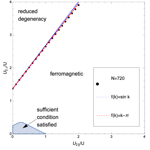
Figure 2: The ground state phase diagram of Eq. (15) at half filling on the $U_{2\parallel}/U$-$U_{2\angle}/U$ plane. The ground states are ferromagnetic below the phase boundary, and have reduced degeneracy above the boundary. The boundary is obtained by exact diagonalization in a system with $N=720$ in the $S_{z}=N/2-1$ sector, and is well approximated by the two straight lines corresponding to the trial wave functions $f\left(k\right)\propto\sin k$ and $f\left(k\right)\propto k-\pi$ (see text). Also shown is the much smaller region where the sufficient condition for ferromagnetic ground states, Eq. (17), is satisfied.

In Fig. 3, choosing a fixed $U_{2\parallel}/U$, we plot $E_{\text{GS}}\left(S_{z}\right)$ (the ground state energy in the sector labeled by $S_{z}$) as a function of $\left|S_{z}\right|$ for different $U_{2\angle}/U$ outside of the ferromagnetic regime. We observe that $E_{\text{GS}}\left(S_{z}\right)$ is a monotonically increasing function of $\left|S_{z}\right|$ in general, and becomes a strictly increasing function of $\left|S_{z}\right|$ if $U_{2\angle}\$is sufficiently large. This property of $E_{\text{GS}}\left(S_{z}\right)$ allows us to determine the ferromagnetic phase boundary in Fig. 2 by calculating $E_{\text{GS}}\left(S_{z}=N/2-1\right)$, which for a given $N$ is considerably less numerically intensive than $E_{\text{GS}}\left(S_{z}=0\right)$. Reasonably accurate estimates of the phase boundary can then be made through a variational calculation. We can characterize an arbitrary $Q=0$ state in the $S_{z}=N/2-1$ sector by

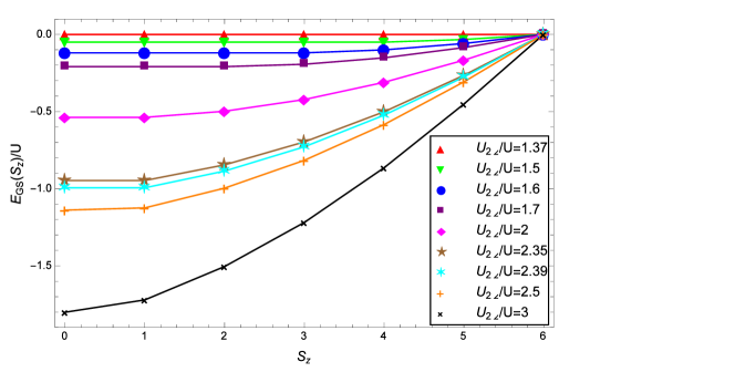
Figure 3: The ground state energy in the $S_{z}$ sector, $E_{GS}\left(S_{z}\right)$, versus $\left|S_{z}\right|$ for $U_{2\parallel}=0$ and various $U_{2\angle}/U$ outside of the ferromagnetic regime. The results are obtained by exact diagonalization in a system with $N=12$.

$$\int_{\frac{2\pi}{3}}^{\frac{4\pi}{3}}dkf\left(k\right)e_{k,\uparrow}e_{k,\downarrow}^{{\dagger}}\left|\text{FM}\uparrow\right\rangle\text{.}$$ (18)

The ferromagnetic state in this sector corresponds to $f\left(k\right)=1$, i.e. an equal-weighted superposition of all states where every edge state is singly occupied. The energy expectation value as a functional of $f$ is a linear combination of $U$, $U_{2\parallel}$ and $U_{2\angle}$:

$$E\left[f\right]=UC_{0}\left[f\right]+U_{2\parallel}C_{2\parallel}\left[f\right]+U_{2\angle}C_{2\angle}\left[f\right]\text{.}$$ (19)

If $E\left[f\right]<0$, the ground states cannot be the ferromagnetic multiplet whose energy is always zero. For $f\left(k\right)\propto\sin k$, $C_{0}=0.100$, $C_{2\parallel}=0.0964$ and $C_{2\angle}=-0.0730$; for $f\left(k\right)\propto k-\pi$, $C_{0}=0.0946$, $C_{2\parallel}=0.0887$ and $C_{2\angle}=-0.0687$. For these two trial wave functions, the trajectories above which $E\left[f\right]<0$ are plotted in Fig. 2; both trajectories are very close to the ferromagnetic phase boundary obtained from exact diagonalization.

It should also be cautioned that anisotropy is not necessary to stabilize non-ferromagnetic ground states. For instance, we can also study an isotropic interaction consisting of an on-site term and six fifth-nearest-neighbor terms (or equivalently, next-nearest-neighbor terms on the same sublattice):

$$U_{\left(0,0\right)}\equiv U\text{, }U_{\left(0,\pm 2\right)}=U_{\left(\pm 3,1\right)}=U_{\left(\pm 3,-1\right)}\equiv U_{5}\text{,}$$ (20)

and $U_{\left(\delta_{m},\delta_{n}\right)}=0$ for other $\left(\delta_{m},\delta_{n}\right)$. For this model

$$\tilde{U}\left(K,q\right)=U+2U_{5}\left(\cos 2K+2\cos K\cos\frac{3q}{2}\right)\text{,}$$ (21)

so our sufficient condition for ferromagnetism becomes $U_{5}\leq U/3$. In a system with $N=720$, exact diagonalization shows that a non-ferromagnetic ground state appears when $U_{5}>80.48U$, i.e. when the non-local $U_{5}$ term is far stronger than the on-site interaction.

Our exact diagonalization results for both models indicate that while ferromagnetism is favored by the on-site interaction, it may be destabilized by sufficiently strong non-local interactions. This is in agreement with the findings of Ref. Schüler et al., 2013 that the effective on-site part of the interaction in bulk graphene is reduced by a weighted average of non-local interactions.

We now investigate whether the unscreened Coulomb interaction, Eq. (6), satisfies the sufficient condition for ferromagnetism. To this end, we introduce a long-distance cutoff $R$, and minimize $\tilde{U}\left(K,q\right)$ for the interaction that is given by Eq. (6) for $\left|\vec{\delta}\right|\leq R$ but vanishes for $\left|\vec{\delta}\right|>R$. In Fig. 4 we show $\tilde{U}_{\min}$, the minimum of $\tilde{U}\left(K,q\right)$ for $0\leq K\leq\pi$ and $-2\pi/3\leq q\leq 2\pi/3$, as a function of $R$ for $R\leq 500$. While $\tilde{U}_{\min}$ oscillates wildly, its lower envelope is an increasing function of $R$, and $\tilde{U}_{\min}$ does not go below $0.2U_{0}$ for $50\leq R\leq 500$. This strongly implies that $\tilde{U}_{\min}$ remains positive as $R\rightarrow\infty$, and provides evidence that the ferromagnetic multiplet states are the unique ground states for the unscreened Coulomb interaction.

Figure 4: The minimum of $\tilde{U}\left(K,q\right)$ for $0\leq K\leq\pi$ and $-2\pi/3\leq q\leq 2\pi/3$, $\tilde{U}_{\min}$, versus $R$, the long-distance cutoff introduced artificially in the Coulomb interaction Eq. (6).

A remark is in order about the short-distance cutoff $d=1/\left(2\sqrt{3}\right)$ in Eq. (6). If $d$ is treated as a tunable parameter of our model, then the observation that $\tilde{U}_{\min}\left(R\rightarrow\infty\right)>0$ is only valid when $d\lesssim 1$. If $d$ is close to $1$, $\tilde{U}_{\min}$ oscillates around zero even for $R$ up to $500$. Nevertheless, as shown in the next-nearest-neighbor model and the fifth-nearest-neighbor model, violation of the sufficient condition for ferromagnetism $\tilde{U}_{\min}\geq 0$ is not an indication of ground states being non-ferromagnetic. Indeed, we have verified in the $S_{z}=N/2-1$ sector that the ground states remain ferromagnetic for $R$ up to $20$ and $d$ up to $10$.

IV Low-energy excitations

In this section we discuss the low-energy single-particle, single-hole and particle-hole excitations of the ferromagnetic ground state, and also the effect of the particle-hole symmetry breaking term $\Delta$.

It is simplest to consider the excitations from the maximum $S_{z}$ state $\left|\text{FM}\uparrow\right\rangle$. We can rewrite the projected Hamiltonian of Eq. (10) in a form which explicitly annihilates $\left|\text{FM}\uparrow\right\rangle$:

$$H_{\text{int}} = \int dk\left[\epsilon_{p}\left(k\right)e_{k,\downarrow}^{{\dagger}}e_{k,\downarrow}+\epsilon_{h}\left(k\right)e_{k,\uparrow}e_{k,\uparrow}^{{\dagger}}\right]-\int\frac{dkdk^{\prime}dq}{2\pi}\Gamma\left(k,k^{\prime},q\right)e_{k,\uparrow}e_{k^{\prime}-q,\downarrow}^{{\dagger}}e_{k^{\prime},\downarrow}e_{k+q,\uparrow}^{{\dagger}}$$ (22)

$$+\frac{1}{2}\int\frac{dkdk^{\prime}dq}{2\pi}\Gamma\left(k,k^{\prime},q\right)\left(e_{k+q,\downarrow}^{{\dagger}}e_{k^{\prime}-q,\downarrow}^{{\dagger}}e_{k^{\prime},\downarrow}e_{k,\downarrow}+e_{k+q,\uparrow}e_{k^{\prime}-q,\uparrow}e_{k^{\prime},\uparrow}^{{\dagger}}e_{k,\uparrow}^{{\dagger}}\right)\text{,}$$

where the domains of integration are such that all edge states have momenta between $2\pi/3$ and $4\pi/3$, the interaction kernel is

$$\Gamma\left(k,k^{\prime},q\right)$$ (23)

$$= \frac{g_{0}\left(k\right)g_{0}\left(k^{\prime}\right)g_{0}\left(k+q\right)g_{0}\left(k^{\prime}-q\right)}{1-16\cos\frac{k}{2}\cos\frac{k+q}{2}\cos\frac{k^{\prime}}{2}\cos\frac{k^{\prime}-q}{2}}\frac{1}{2}\sum_{\delta_{m},\delta_{n}}U_{\left(\delta_{m},\delta_{n}\right)}\cos\frac{q\delta_{m}}{2}$$

$$\times\left[\left(4\cos\frac{k^{\prime}}{2}\cos\frac{k^{\prime}-q}{2}\right)^{\left|\delta_{n}\right|}+\left(4\cos\frac{k}{2}\cos\frac{k+q}{2}\right)^{\left|\delta_{n}\right|}\right]\text{,}$$

and the energy to create one single spin-down electron or one single spin-up hole is

$$\epsilon_{p/h}\left(k\right)=\frac{1}{2}\int_{\frac{2\pi}{3}}^{\frac{4\pi}{3}}\frac{dk^{\prime}}{2\pi}\Gamma\left(k,k^{\prime},k^{\prime}-k\right)\pm\Delta\left(2\cos k+1\right)\text{.}$$ (24)

As noted in Refs. Luitz et al., 2011; Karimi and Affleck, 2012, the interaction $\Gamma\left(k,k^{\prime},q\right)$ is strongly momentum-dependent. For both Hubbard and Coulomb interactions, $\Gamma\left(k,k^{\prime},q\right)$ is positive so that spin-down electrons attract spin-down holes, which favors the formation of bound states between the two. The third term in Eq. (22) generally gives rise to interaction between edge states with the same spin orientation, although for the Hubbard model it vanishes due to an additional symmetry of the kernel, $\Gamma\left(k,k^{\prime},q\right)=\Gamma\left(k,k^{\prime},k^{\prime}-k-q\right)$.

IV.1 Single particle and single hole excitations

We first examine the eigenstates deviating slightly from half-filling, namely the single particle excitations and single hole excitations. They are represented by $e_{k,\downarrow}^{{\dagger}}\left|\text{FM}\uparrow\right\rangle$ [of energy $\epsilon_{p}\left(k\right)$] and $e_{k,\uparrow}\left|\text{FM}\uparrow\right\rangle$ [of energy $\epsilon_{h}\left(k\right)$] respectively. Using the definitions Eqs. (24) and (23) and the fact that $\delta_{n}+\delta_{m}$ is even, it is easy to show that $\epsilon_{p/h}\left(k\right)=\epsilon_{p/h}\left(2\pi-k\right)$, so we may focus on $2\pi/3\leq k\leq\pi$.

Near the Dirac point $0<k-2\pi/3\ll 1$, we can expand Eq. (24) to obtain

$$\epsilon_{p/h}\left(k\right)\approx\left(v\mp\sqrt{3}\Delta\right)\left(k-\frac{2\pi}{3}\right)\text{,}$$ (25)

where the velocity $v$ depends only on the interactions:

$$v\equiv\frac{\sqrt{3}}{2}\sum_{\delta_{m},\delta_{n}}U_{\left(\delta_{m},\delta_{n}\right)}\int_{\frac{2\pi}{3}}^{\frac{4\pi}{3}}\frac{dk^{\prime}}{2\pi}\left(2\cos\frac{k^{\prime}}{2}\right)^{\left|\delta_{n}\right|}\cos\left(k^{\prime}-\frac{2\pi}{3}\right)\frac{\delta_{m}}{2}\text{.}$$ (26)

Since the $k^{\prime}$ integral is finite, $v$ is finite for any short-range interaction. Eq. (25) shows that, as in the projected Hubbard model,Karimi and Affleck (2012) the single-particle and single-hole excitations are generally gapless at the Dirac points for a single zigzag edge.

For the next-nearest-neighbor model Eq. (15), $v$ is always positive:

$$v=\frac{\sqrt{3}}{6}U+\frac{3}{4\pi}U_{2\parallel}+\left(\frac{1}{\sqrt{3}}-\frac{3}{2\pi}\right)U_{2\angle}\text{.}$$ (27)

Nevertheless, $v$ may become negative for certain strongly non-local interactions. An example is the term with $\delta_{m}=4$ and $\delta_{n}=0$, which gives a coefficient of $-3/\left(16\pi\right)$. The ferromagnetic ground state will be unstable against the creation of electrons or holes near the Dirac points in the case of $v<0$, or more generally $v<\sqrt{3}\left|\Delta\right|$ when the particle-hole symmetry breaking term $\Delta$ is nonzero.

The case of unscreened Coulomb interaction Eq. (6) is especially interesting. In this case the low-energy behavior of $\epsilon_{p/h}\left(k\right)$ is controlled by the long range part of $U_{\left(\delta_{m},\delta_{n}\right)}$. When $\left|\delta_{n}\right|\gg 1$ or $\left|\delta_{m}\right|\gg 1$, the $k^{\prime}$ integral is dominated by $k^{\prime}$ near the Dirac points, and we findPereira et al. (2006)

$$\int_{\frac{2\pi}{3}}^{\frac{4\pi}{3}}\frac{dk^{\prime}}{2\pi}\left(2\cos\frac{k^{\prime}}{2}\right)^{\left|\delta_{n}\right|}\cos\left(k^{\prime}-\frac{2\pi}{3}\right)\frac{\delta_{m}}{2}$$ (28)

$$\approx \frac{1}{2\pi}\operatorname{Re}\left[\frac{2}{\sqrt{3}\left|\delta_{n}\right|-i\delta_{m}}+\left(-1\right)^{\left|\delta_{n}\right|}e^{i\frac{\pi}{3}\delta_{m}}\frac{2}{\sqrt{3}\left|\delta_{n}\right|+i\delta_{m}}\right]\text{.}$$

Approximating the sum over $\delta_{n}$ and $\delta_{m}$ by integrals over $x=\delta_{m}/2$ and $y=\sqrt{3}\delta_{n}/2$, and discarding the subleading contribution from the oscillating term, we see that $v\propto\ln R$ where $R$ is the long-distance cutoff:

$$v \approx \int dx\int dy\frac{U_{0}d}{\sqrt{x^{2}+y^{2}}}\frac{1}{2\pi}\frac{\left|y\right|}{x^{2}+y^{2}}$$ (29)

$$\approx \frac{U_{0}d}{2\pi}\int_{0}^{2\pi}d\theta\left|\sin\theta\right|\int_{d}^{R}\frac{dr}{r}=\frac{2U_{0}d}{\pi}\ln\frac{R}{d}\text{.}$$

As $R\rightarrow\infty$, the only other large distance scale in the problem is given by the inverse distance to the Dirac points, which should therefore replace $R$ as the distance cutoff. In other words, for the unscreened Coulomb interaction, $\epsilon_{p/h}$ has the following behavior for $0<k-2\pi/3\ll 1$:

$$\epsilon_{p/h}\left(k\right)\approx\frac{2U_{0}d}{\pi}\left(k-\frac{2\pi}{3}\right)\ln\frac{\Lambda}{k-\frac{2\pi}{3}}\text{,}$$ (30)

where $\Lambda\ll 1$ is a momentum cutoff. This behavior is not affected by the particle-hole symmetry breaking term $\Delta$, which merely shifts $\Lambda$.

In Fig. 5 we plot $\epsilon_{p/h}\left(k\right)/\left(k-2\pi/3\right)$ versus $\ln\left(k-2\pi/3\right)$ at $0<k-2\pi/3\ll 1$ for the Coulomb interaction with various $R$, and show how the logarithmic divergence in Eq. (30) is cut off at low energies by $R$. We also plot the velocity $v$ given by Eq. (26) as a function of $\ln R$ in Fig. 6. These results suggest that the Coulomb interaction produces a divergent “Fermi velocity” for edge modes near the Dirac points, a behavior reminiscent of the marginal Fermi liquid in bulk graphene with Coulomb interaction.González et al. (1999)

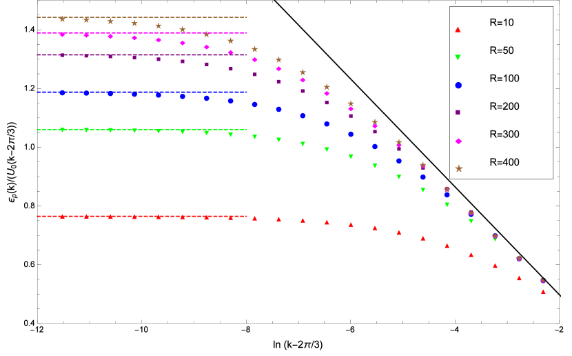
Figure 5: The single-particle/single-hole dispersion for the Coulomb interaction near the Dirac point. $\epsilon_{p/h}\left(k\right)/\left(U_{0}\left(k-2\pi/3\right)\right)$ is plotted against $\ln\left(k-2\pi/3\right)$ for $10^{-5}\leq k-2\pi/3\leq 0.1$ and different values of long-distance cutoff $R$, with the particle-hole symmetry breaking perturbation $\Delta$ set to zero. For comparison we also show the velocity given by Eq. (26) for each $R$ as a horizontal line. The black line has a slope of $2d/\pi$.

Figure 6: The velocity given by Eq. (26) for the Coulomb interaction as a function of the long-distance cutoff $R$. The fitted line has a slope of $0.1836$ while $2d/\pi=0.1838$.

It is also useful to consider $k=\pi$, since this is where $\epsilon_{p/h}\left(k\right)$ obtains its maximum for the Hubbard interaction and the Coulomb interaction, in the absence of particle-hole symmetry breaking. At $k=\pi$ Eq. (24) is again greatly simplified:

$$\epsilon_{p/h}\left(\pi\right) = \mp\Delta+\left(\frac{\sqrt{3}}{2\pi}-\frac{1}{6}\right)U_{\left(0,0\right)}+\left(\frac{1}{6}-\frac{\sqrt{3}}{8\pi}\right)U_{\left(1,0\right)}$$ (31)

$$+\frac{1}{\pi}\sum_{\delta_{m}}^{\prime}U_{\left(\delta_{m},0\right)}\left[\frac{8}{\delta_{m}\left(\delta_{m}^{2}-4\right)}\sin\frac{\pi}{6}\delta_{m}-\frac{4\sqrt{3}}{\delta_{m}^{2}-4}\cos\frac{\pi}{6}\delta_{m}\right]\text{,}$$

where the sum is over even $\delta_{m}$ with $\delta_{m}\geq 4$.

$\epsilon_{p/h}\left(\pi\right)$ is also finite for any short-range interaction. Interestingly, $\epsilon_{p/h}\left(\pi\right)$ depends on $U_{\left(\delta_{m},\delta_{n}\right)}$ only if $\delta_{n}=0$: it is, for instance, independent of $U_{2\angle}$ in the next-nearest-neighbor model Eq. (15). For the Coulomb interaction Eq. (6), the $\delta_{m}$ sum turns out to be convergent, and we find

$$\epsilon_{p/h}\left(\pi\right)\approx\mp\Delta+0.189U_{0}$$ (32)

where $U_{0}$ is the on-site interaction strength. Therefore, when $\Delta>\Delta_{c}\left(R\rightarrow\infty\right)=0.189U_{0}$ for the unscreened Coulomb interaction, the maximum $S_{z}$ state $\left|\text{FM}\uparrow\right\rangle$ becomes unstable towards the creation of a spin-down electron at $k=\pi$, e.g. by absorption from the bulk. [For Hubbard interaction with strength $U$, the condition is $\Delta>\Delta_{c}\left(R=0\right)=\left(\sqrt{3}/\left(2\pi\right)-1/6\right)U\approx 0.109U$.]Karimi and Affleck (2012) Similarly, when $\Delta<-\Delta_{c}\left(R\rightarrow\infty\right)$ there is an instability towards the creation of a spin-up hole at $k=\pi$.

In Fig. 7 we plot $\epsilon_{p}\left(k\right)$ versus $k$ for $2\pi/3\leq k\leq 4\pi/3$ for the Coulomb interaction with different values of long-distance cutoff $R$, both when $\Delta=0$ and when $\Delta=\Delta_{c}\left(R\right)$ so that $\epsilon_{p}\left(\pi\right)$ vanishes. Notice that for the Coulomb interaction $\epsilon_{p}\left(k\right)>0$ for $0<k-2\pi/3\ll 1$ even when $\Delta=\Delta_{c}\left(R\right)$; that is, as we increase $\left|\Delta\right|$, single particle or single hole creation energy becomes negative at $k=\pi$ sooner than it does near the Dirac points.

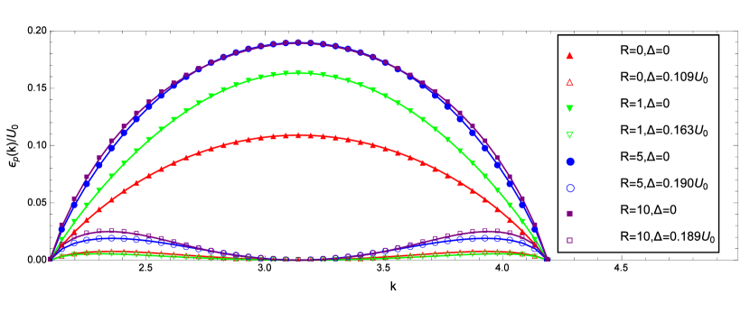
Figure 7: The single-particle dispersion for the Coulomb interaction. $\epsilon_{p}\left(k\right)/U_{0}$ is plotted against $k$ for $2\pi/3\leq k\leq 4\pi/3$ and different values of long-distance cutoff $R$. The particle-hole symmetry breaking perturbation $\Delta$ is either $0$ (filled symbols) or $\Delta_{c}\left(R\right)$ (empty symbols).

IV.2 1-particle-1-hole sector

We turn to the half-filled sector with $N-1$ spin-up electrons and $1$ spin-down electron, so that $S_{z}=N/2-1$. This sector hosts $1$ spin-down electron and $1$ spin-up hole relative to the $\left|\text{FM}\uparrow\right\rangle$ state, and accommodates the excitations that would be seen as magnons in an effective spin model.

Let the total momentum relative to $\left|\text{FM}\uparrow\right\rangle$ be $Q$, and without loss of generality we assume $Q\geq 0$. Denoting an eigenstate by

$$\int_{\frac{2\pi}{3}}^{\frac{4\pi}{3}-Q}dkf\left(k;Q\right)e_{k,\uparrow}e_{k+Q,\downarrow}^{{\dagger}}\left|\text{FM}\uparrow\right\rangle\text{,}$$ (33)

we obtain the following Schroedinger’s equation:

$$\left[E-\epsilon_{h}\left(k\right)-\epsilon_{p}\left(k+Q\right)\right]f\left(k;Q\right)=-\int\frac{dk^{\prime}}{2\pi}\Gamma\left(k,k^{\prime}+Q,k^{\prime}-k\right)f\left(k^{\prime};Q\right)\text{,}$$ (34)

where $E$ is the energy eigenvalue. The ferromagnetic state in the 1-particle-1-hole sector, $f\left(k;Q=0\right)=1$, is obviously a zero-energy solution.

It is possible for $f\left(k,Q\right)$ to have a $\delta$-function peak at $k=k_{0}$. In this case the solution to Eq. (34) is part of the 1-particle-1-hole continuum, and has an energy $E=\epsilon_{h}\left(k_{0}\right)+\epsilon_{p}\left(k_{0}+Q\right)$. Another possibility is having $E<\epsilon_{h}\left(k\right)+\epsilon_{p}\left(k+Q\right)$ for any $k$, in which case $f\left(k;Q\right)$ does not have any $\delta$-function peaks, and the solution is a particle-hole bound state, or an exciton. Since it reduces $S_{z}$ by $1$, it can also be viewed as a magnon in an effective spin model.

For any short range interaction, we can show that the exciton energy has the following $Q\ll 1$ behavior:

$$E\left(Q\right)=\frac{3v}{2\pi}\left(1-\frac{3\Delta^{2}}{v^{2}}\right)Q^{2}\ln\frac{\Lambda^{\prime}}{Q}\text{,}$$ (35)

where $v$ is the velocity Eq. (26) that also appears in the single particle dispersion, and $\Lambda^{\prime}\ll 1$ is again a momentum cutoff. The inverse exciton mass, or the spin stiffness of the ferromagnetic zigzag edge, is therefore logarithmically divergent. The derivation of Eq. (35) is sketched in Appendix A, where we see the divergence arises due to the linear behavior of $\epsilon_{p/h}\left(k\right)$ near the Dirac points. This divergence is possibly related to the large spin stiffness found by Refs. Yazyev and Katsnelson, 2008; Rhim and Moon, 2009 for $U$ comparable to $t$.

Although similar exciton dispersions have been previously reported in carbon nanotubes,Jiang et al. (2007); *PhysRevLett.106.136805; *PhysRevLett.109.187403 in contrast to Eq. (35) they originate from the long-range nature of the Coulomb interaction. In fact, since in the Coulomb interaction with a long-distance cutoff $R$ we have $v\propto\ln R$, we expect that Eq. (35) is modified to $E\left(Q\right)\propto Q^{2}\ln^{2}Q$ for $R\rightarrow\infty$; that is, the spin stiffness is even more divergent than a logarithm for the unscreened Coulomb interaction. Fig. 8 shows $E\left(Q\right)/Q^{2}$ plotted against $\ln Q$ at $0<Q\ll 1$ for some values of $R$ and $\Delta=0$, where $E\left(Q\right)$ is found by solving Eq. (34) numerically via Chebyshev series expansion.Abramowitz and Stegun (2012)

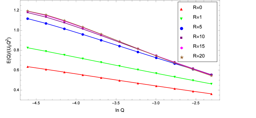
Figure 8: The exciton dispersion for the Coulomb interaction at small momenta. $E\left(Q\right)/\left(U_{0}Q^{2}\right)$ is plotted against $\ln Q$ for $0.01\leq Q\leq 0.1$ and different values of long-distance cutoff $R$, with the particle-hole symmetry breaking perturbation $\Delta$ set to zero. The lowest $100$ Chebyshev polynomials are retained in the numerical solution.

It is also helpful to examine the effect of $\Delta$ on the exciton dispersion, taking as an example the Coulomb interaction with a long-distance cutoff $R$. As depicted in Fig. 9, when $\left|\Delta\right|=\Delta_{c}\left(R\right)$ so that $\epsilon_{p}\left(\pi\right)=0$, the exciton dispersion $E\left(Q\right)$ calculated numerically also approximately vanishes at $Q=\pm\pi/3$, and the exciton wave function strongly favors the state with a spin-down electron at $\pi$ and a spin-up hole at either Dirac point. For $\left|\Delta\right|>\Delta_{c}\left(R\right)$, in parallel with the Hubbard case,Karimi and Affleck (2012) $E\left(\pm\pi/3\right)$ becomes negative which indicates that the ground state at half-filling is no longer maximally spin polarized; instead, the edge states near $\pi$ become more likely to be doubly occupied and the edge states near the Dirac points become more likely to be unoccupied.

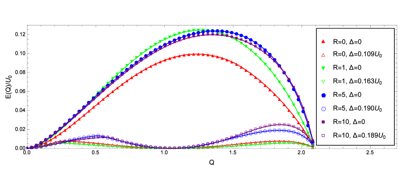
Figure 9: The exciton dispersion for the Coulomb interaction. $E\left(Q\right)/U_{0}$ is plotted against $Q$ for $0\leq Q\leq 2\pi/3$ and different values of long-distance cutoff $R$. The particle-hole symmetry breaking perturbation $\Delta$ is either $0$ (filled symbols) or $\Delta_{c}\left(R\right)$ (empty symbols). The lowest $100$ Chebyshev polynomials are retained in the numerical solution.

Finally, we mention that in the 2-particle-2-hole sector, the excitons in the 1-particle-1-hole sector can form an additional bound state below the exciton continuum. Nevertheless, for both the Hubbard and the Coulomb interactions with $\left|\Delta\right|<\Delta_{c}\left(R\right)$, we find numerically that the bottom of the 2-particle-2-hole bound state dispersion remains positive; we thus conjecture that the ferromagnetic ground state is stable for $\left|\Delta\right|$ up to $\Delta_{c}\left(R\right)$. We also mention that the bound state picture provides an intuitive explanation for the non-ferromagnetic regime in Fig. 3: for $M<N/2$, we can usually form an $M$-particle-$M$-hole bound state with a non-negative binding energy, i.e. with an energy lower than or equal to the sum of energies of an $\left(M-1\right)$-particle-$\left(M-1\right)$-hole bound state and a 1-particle-1-hole bound state. Therefore, if the 1-particle-1-hole ground state has a negative energy as happens for sufficiently large $U_{2\angle}$, then as $M$ increases and $\left|S_{z}\right|$ decreases, the ground state energy in the $S_{z}$ sector either stays the same or decreases.

V Discussion and conclusions

In our effective model Eq. (8) at $O\left(U\right)$, we have ignored the dynamics of low-lying bulk degrees of freedom near the Dirac points, so an obvious issue is whether this approximation is justified. For the on-site Hubbard interaction, the answer is partly given by Refs. Karimi and Affleck, 2012; Koop and Schmidt, 2015, where effective Hamiltonians are found to $O\left(U^{2}/t\right)$ by integrating out the bulk states and neglecting retardation. While Ref. Karimi and Affleck, 2012 finds that the $O\left(U^{2}/t\right)$ correction to the Hamiltonian has a $q^{2}\ln q$ behavior for small momentum transfer $q$, such behavior does not necessarily hint at a breakdown of the perturbation theory, as logarithms also appear at $O\left(U\right)$, e.g. in the exciton dispersion Eq. (35). Ref. Koop and Schmidt, 2015 further shows that, as far as the effective spin model is concerned, the interaction strengths are only weakly modified by the bulk states even for $U$ comparable to $t$. In other words, there is no evidence that the perturbation theory in $U/t$ is divergent. However, while a weak Hubbard interaction is known to be irrelevant in the bulk, a weak Coulomb interaction is marginally irrelevant and may lead to further logarithmic corrections.González et al. (1999); Kotov et al. (2012) It therefore remains an open question whether integrating out the bulk states at $O\left(U^{2}/t\right)$ qualitatively changes the physics of the $O\left(U\right)$ edge model for the unscreened Coulomb interaction.

Another problem that we have not discussed so far is the inter-edge coupling in realistic graphene nanoribbons. We now consider a ribbon of large but finite width $W\gg 1$ with two zigzag edges, whose overall ground state is antiferromagnetic. The inter-edge coupling originates in part from the direct interaction between opposite edges, which is significant even at the first order in interaction if it is long-ranged [$O\left(U_{0}/W\right)$ in the Coulomb case]. Inter-edge coupling is also mediated by bulk states, which is second order in interaction and is $O\left(U^{2}/\left(tW^{2}\right)\right)$ in the Hubbard case.Karimi and Affleck (2012) Yet another source is the hopping amplitude between edge states of opposite edges, which exists even in the absence of interactions and leads to an energy gap exponentially small in $W$. For wide ribbons $W\gg 1$, it is well known that the edge states are no longer strictly localized near one edge when their momenta are within $O\left(1/W\right)$ of the Dirac points. The hopping amplitude at momentum $k$ thus grows rapidly as $k$ approaches the Dirac points, eventually reaching $O\left(t/W\right)$.Brey and Fertig (2006); Jung et al. (2009) Under our assumption $U\ll t$, this is actually a much larger energy scale than that of the direct inter-edge Coulomb interaction or that of the bulk-mediated inter-edge interaction. Thus it is not justified to ignore the inter-edge hopping amplitude near the Dirac points in the effective model for a nanoribbon. In fact, at the mean-field level, it is exactly the part of the Brillouin zone near the Dirac points that contributes the most to the inter-edge superexchange interaction,Jung et al. (2009); Jung (2011) and the spin wave dispersion becomes linear for small momenta once the inter-edge coupling is taken into account.Culchac et al. (2011) Although an effective edge model incorporating the inter-edge hoppingSchmidt et al. (2013) is often much less analytically accessible beyond the mean-field level, we hope further insight on the effect of Coulomb interaction in finite width nanoribbons can be gleaned from exact diagonalization.

In conclusion, we have investigated the effects of long-range interactions on the zigzag edge states of a semi-infinite graphene sheet. By projecting the interaction onto the edge state subspace, we obtain an effective model for which the states in the maximally polarized ferromagnetic multiplet are zero energy eigenstates. A sufficient condition is found for the ferromagnetic multiplet to be the ground states, and we present evidence that the unscreened Coulomb interaction satisfies this condition, which implies that its ground states are ferromagnetic. In cases where the sufficient condition is not met, exact diagonalization results indicate that the ground state can be non-ferromagnetic, provided that certain non-local components of the interaction are sufficiently strong. We also discuss the single-particle excitations, single-hole excitations and spin-1 excitons of the maximum $S_{z}$ ground state. For short range interactions the single-particle and single-hole excitations have linear dispersions near the Dirac points, as described in Eq. (25). The slope $v$ also governs the exciton energy at small momenta, Eq. (35), which shows a $vQ^{2}\ln Q$ behavior. For the unscreened Coulomb interaction $v$ becomes logarithmically divergent as a function of the long-distance cutoff, corresponding to a $\delta k\ln\delta k$ behavior where $\delta k\ll 1$ is the distance from either of the Dirac points. The edge states acquire a dispersion due to a particle-hole symmetry breaking perturbation $\Delta$; the ferromagnetic ground state can be destroyed if $\left|\Delta\right|$ is large enough.

Appendix A Exciton dispersion at small momenta for a single zigzag edge with short-range interactions

For simplicity, we illustrate the derivation of Eq. (35) with the Hubbard interaction $U_{\left(0,0\right)}=U$. Generalization to non-local interactions is tedious but straightforward; it is briefly discussed at the end of this appendix.

Expanding the denominator of the kernel $\Gamma$ in Eq. (34), we can isolate the $k$ dependence of $f\left(k;Q\right)$:

$$f\left(k;Q\right)=-\frac{g_{0}\left(k\right)g_{0}\left(k+Q\right)}{E-\epsilon_{h}\left(k\right)-\epsilon_{p}\left(k+Q\right)}\sum_{l=0}^{\infty}\left(4\cos\frac{k}{2}\cos\frac{k+Q}{2}\right)^{l}U\Phi_{l}\left(Q\right)\text{,}$$ (36)

where $\Phi$’s are independent of $k$, and are defined as

$$\Phi_{l}\left(Q\right)=\int_{\frac{2\pi}{3}}^{\frac{4\pi}{3}-Q}\frac{dk^{\prime}}{2\pi}g_{0}\left(k^{\prime}+Q\right)g_{0}\left(k^{\prime}\right)\left(4\cos\frac{k^{\prime}}{2}\cos\frac{k^{\prime}+Q}{2}\right)^{l}f\left(k^{\prime};Q\right)\text{.}$$ (37)

Inserting Eq. (36) into Eq. (37), we obtain an infinite number of linear equations satisfied by $\Phi$:

$$\Phi_{l}\left(Q\right) = -\int\frac{dk^{\prime}}{2\pi}\frac{\left(1-4\cos^{2}\frac{k^{\prime}+Q}{2}\right)\left(1-4\cos^{2}\frac{k^{\prime}}{2}\right)}{E-\epsilon_{h}\left(k^{\prime}\right)-\epsilon_{p}\left(k^{\prime}+Q\right)}\left(4\cos\frac{k^{\prime}}{2}\cos\frac{k^{\prime}+Q}{2}\right)^{l}$$ (38)

$$\times\sum_{l^{\prime}=0}^{\infty}\left(4\cos\frac{k^{\prime}}{2}\cos\frac{k^{\prime}+Q}{2}\right)^{l^{\prime}}U\Phi_{l^{\prime}}\left(Q\right)\text{.}$$

For $Q\ll 1$, the integrand on the right-hand side can be expanded to $O\left(E\right)$ and $O\left(Q^{2}\right)$.

$$\Phi_{l}\left(Q\right) = \int\frac{dk^{\prime}}{2\pi}\frac{\left(1-4\cos^{2}\frac{k^{\prime}}{2}\right)^{2}}{\epsilon_{h}\left(k^{\prime}\right)+\epsilon_{p}\left(k^{\prime}\right)}\left(4\cos^{2}\frac{k^{\prime}}{2}\right)^{l}\sum_{l^{\prime}=0}^{\infty}\left(4\cos^{2}\frac{k^{\prime}}{2}\right)^{l^{\prime}}U\Phi_{l^{\prime}}\left(Q\right)$$ (39)

$$+E\int\frac{dk^{\prime}}{2\pi}\frac{\left(1-4\cos^{2}\frac{k^{\prime}}{2}\right)^{2}}{\left[\epsilon_{h}\left(k^{\prime}\right)+\epsilon_{p}\left(k^{\prime}\right)\right]^{2}}\left(4\cos^{2}\frac{k^{\prime}}{2}\right)^{l}\sum_{l^{\prime}=0}^{\infty}\left(4\cos^{2}\frac{k^{\prime}}{2}\right)^{l^{\prime}}U\Phi_{l^{\prime}}\left(0\right)$$

$$+2\int_{\frac{2\pi}{3}}^{\frac{2\pi}{3}+\Lambda}\frac{dk^{\prime}}{2\pi}\frac{-\frac{3}{4}\left(1-\frac{3\Delta^{2}}{v^{2}}\right)Q^{2}}{v\left(2k+Q-\frac{4\pi}{3}\right)-\sqrt{3}\Delta Q}\sum_{l^{\prime}=0}^{\infty}U\Phi_{l^{\prime}}\left(0\right)\text{.}$$

In the second and the third lines we have approximated $\Phi_{l^{\prime}}\left(Q\right)\approx\Phi_{l^{\prime}}\left(0\right)$, assuming that $\Phi_{l}\left(Q\right)$ is well-behaved at $Q=0$ and any difference is $O\left(Q\right)$. In the third line we have retained the most singular contribution at $O\left(Q^{2}\right)$, which are from the vicinity of the Dirac points (hence the factor of $2$), as the remaining terms contain no infrared divergence.

Using Eq. (37) and recalling that the $Q=0$ solution is $f\left(k;0\right)=1$, we have

$$\sum_{l^{\prime}=0}^{\infty}U\Phi_{l^{\prime}}\left(0\right)=\sum_{l^{\prime}=0}^{\infty}\int_{\frac{2\pi}{3}}^{\frac{4\pi}{3}}\frac{dk}{2\pi}g_{0}^{2}\left(k\right)U\left(4\cos^{2}\frac{k}{2}\right)^{l^{\prime}}=\frac{U}{3}\text{,}$$ (40)

and

$$\sum_{l^{\prime}=0}^{\infty}\left(4\cos^{2}\frac{k^{\prime}}{2}\right)^{l^{\prime}}U\Phi_{l^{\prime}}\left(0\right)=\sum_{l^{\prime}=0}^{\infty}\int_{\frac{2\pi}{3}}^{\frac{4\pi}{3}}\frac{dk}{2\pi}g_{0}^{2}\left(k\right)U\left(16\cos^{2}\frac{k}{2}\cos^{2}\frac{k^{\prime}}{2}\right)^{l^{\prime}}=\frac{\epsilon_{h}\left(k^{\prime}\right)+\epsilon_{p}\left(k^{\prime}\right)}{1-4\cos^{2}\frac{k^{\prime}}{2}}\text{;}$$ (41)

therefore

$$\Phi_{l}\left(Q\right) = \int\frac{dk^{\prime}}{2\pi}\frac{\left(1-4\cos^{2}\frac{k^{\prime}}{2}\right)^{2}}{\epsilon_{h}\left(k^{\prime}\right)+\epsilon_{p}\left(k^{\prime}\right)}\left(4\cos^{2}\frac{k^{\prime}}{2}\right)^{l}\sum_{l^{\prime}=0}^{\infty}\left(4\cos^{2}\frac{k^{\prime}}{2}\right)^{l^{\prime}}U\Phi_{l^{\prime}}\left(Q\right)$$ (42)

$$+E\int\frac{dk^{\prime}}{2\pi}\frac{1-4\cos^{2}\frac{k^{\prime}}{2}}{\epsilon_{h}\left(k^{\prime}\right)+\epsilon_{p}\left(k^{\prime}\right)}\left(4\cos^{2}\frac{k^{\prime}}{2}\right)^{l}-\frac{1}{8\pi v}\left(1-\frac{3\Delta^{2}}{v^{2}}\right)Q^{2}U\ln\frac{\Lambda^{\prime}}{Q}\text{.}$$

Now, we multiply the entire expression by $\left[1-4\cos^{2}\left(k/2\right)\right]\left[4\cos^{2}\left(k/2\right)\right]^{l}U$, then sum over $l$ and integrate over $k$. The left hand side then cancels the first term on the right hand side, and using $v=U/\left(2\sqrt{3}\right)$, we are left with Eq. (35).

In the presence of non-local interactions, one needs to assign three more indices to $\Phi$, namely $\delta_{m}$, $\delta_{n}$ and $\alpha=1$, $2$ [corresponding to the two terms in the third line of Eq. (23)]. All three indices should be summed over in Eq. (38), and subsequently in Eqs. (40), (41) and (42).

References

- Fujita et al. (1996) M. Fujita, K. Wakabayashi, K. Nakada, and K. Kusakabe, Journal of the Physical Society of Japan 65, 1920 (1996).
- Wakabayashi et al. (2010) K. Wakabayashi, K. ichi Sasaki, T. Nakanishi, and T. Enoki, Science and Technology of Advanced Materials 11, 054504 (2010).
- Yazyev (2010) O. V. Yazyev, Reports on Progress in Physics 73, 056501 (2010).
- Yamashiro et al. (2003) A. Yamashiro, Y. Shimoi, K. Harigaya, and K. Wakabayashi, Phys. Rev. B 68, 193410 (2003).
- Jung et al. (2009) J. Jung, T. Pereg-Barnea, and A. H. MacDonald, Phys. Rev. Lett. 102, 227205 (2009).
- Jung and MacDonald (2009) J. Jung and A. H. MacDonald, Phys. Rev. B 79, 235433 (2009).
- Rhim and Moon (2009) J.-W. Rhim and K. Moon, Phys. Rev. B 80, 155441 (2009).
- Schmidt and Loss (2010) M. J. Schmidt and D. Loss, Phys. Rev. B 82, 085422 (2010).
- Jung (2011) J. Jung, Phys. Rev. B 83, 165415 (2011).
- Culchac et al. (2011) F. J. Culchac, A. Latgé, and A. T. Costa, New Journal of Physics 13, 033028 (2011).
- Schmidt (2012) M. J. Schmidt, Phys. Rev. B 86, 075458 (2012).
- Karimi and Affleck (2012) H. Karimi and I. Affleck, Phys. Rev. B 86, 115446 (2012).
- Luitz et al. (2011) D. J. Luitz, F. F. Assaad, and M. J. Schmidt, Phys. Rev. B 83, 195432 (2011).
- Schmidt et al. (2013) M. J. Schmidt, M. Golor, T. C. Lang, and S. Wessel, Phys. Rev. B 87, 245431 (2013).
- Wunsch et al. (2008) B. Wunsch, T. Stauber, F. Sols, and F. Guinea, Phys. Rev. Lett. 101, 036803 (2008).
- Golor et al. (2013a) M. Golor, T. C. Lang, and S. Wessel, Phys. Rev. B 87, 155441 (2013a).
- Golor et al. (2013b) M. Golor, C. Koop, T. C. Lang, S. Wessel, and M. J. Schmidt, Phys. Rev. Lett. 111, 085504 (2013b).
- Golor et al. (2014) M. Golor, S. Wessel, and M. J. Schmidt, Phys. Rev. Lett. 112, 046601 (2014).
- Hagymási and Legeza (2016) I. Hagymási and O. Legeza, Phys. Rev. B 94, 165147 (2016).
- Son et al. (2006) Y.-W. Son, M. L. Cohen, and S. G. Louie, Phys. Rev. Lett. 97, 216803 (2006).
- Pisani et al. (2007) L. Pisani, J. A. Chan, B. Montanari, and N. M. Harrison, Phys. Rev. B 75, 064418 (2007).
- Huang et al. (2013) L. F. Huang, G. R. Zhang, X. H. Zheng, P. L. Gong, T. F. Cao, and Z. Zeng, Journal of Physics: Condensed Matter 25, 055304 (2013).
- Wakabayashi et al. (1998) K. Wakabayashi, M. Sigrist, and M. Fujita, Journal of the Physical Society of Japan 67, 2089 (1998).
- Yazyev and Katsnelson (2008) O. V. Yazyev and M. I. Katsnelson, Phys. Rev. Lett. 100, 047209 (2008).
- Zhang et al. (2010) Y.-T. Zhang, H. Jiang, Q.-f. Sun, and X. C. Xie, Phys. Rev. B 81, 165404 (2010).
- Magda et al. (2014) G. Z. Magda, X. Jin, I. Hagymási, P. Vancsó, Z. Osváth, P. Nemes-Incze, C. Hwang, L. P. Biró, and L. Tapasztó, Nature 514, 608 (2014).
- Ruffieux et al. (2015) P. Ruffieux, S. Wang, B. Yang, C. Sánchez-Sánchez, J. Liu, T. Dienel, L. Talirz, P. Shinde, C. A. Pignedoli, D. Passerone, T. Dumslaff, X. Feng, K. Müllen, and R. Fasel, Nature 531, 489 (2015).
- Makarova et al. (2015) T. L. Makarova, A. L. Shelankov, A. A. Zyrianova, A. I. Veinger, T. V. Tisnek, E. Lähderanta, A. I. Shames, A. V. Okotrub, L. G. Bulusheva, G. N. Chekhova, D. V. Pinakov, I. P. Asanov, and Z̆. S̆ljivanc̆anin, Sci. Rep. 5, 13382 (2015).
- Lieb (1989) E. H. Lieb, Phys. Rev. Lett. 62, 1201 (1989).
- DiVincenzo and Mele (1984) D. P. DiVincenzo and E. J. Mele, Phys. Rev. B 29, 1685 (1984).
- Kotov et al. (2012) V. N. Kotov, B. Uchoa, V. M. Pereira, F. Guinea, and A. H. Castro Neto, Rev. Mod. Phys. 84, 1067 (2012).
- Wu and Tremblay (2014) W. Wu and A.-M. S. Tremblay, Phys. Rev. B 89, 205128 (2014).
- Herbut (2006) I. F. Herbut, Phys. Rev. Lett. 97, 146401 (2006).
- Honerkamp (2008) C. Honerkamp, Phys. Rev. Lett. 100, 146404 (2008).
- Schüler et al. (2013) M. Schüler, M. Rösner, T. O. Wehling, A. I. Lichtenstein, and M. I. Katsnelson, Phys. Rev. Lett. 111, 036601 (2013).
- Chacko et al. (2014) S. Chacko, D. Nafday, D. G. Kanhere, and T. Saha-Dasgupta, Phys. Rev. B 90, 155433 (2014).
- Zhu and Wang (2006) L. Y. Zhu and W. Z. Wang, Journal of Physics: Condensed Matter 18, 6273 (2006).
- Mermin and Wagner (1966) N. D. Mermin and H. Wagner, Phys. Rev. Lett. 17, 1133 (1966).
- Egger and Gogolin (1997) R. Egger and A. O. Gogolin, Phys. Rev. Lett. 79, 5082 (1997).
- Zarea and Sandler (2007) M. Zarea and N. Sandler, Phys. Rev. Lett. 99, 256804 (2007).
- Zarea et al. (2008) M. Zarea, C. Büsser, and N. Sandler, Phys. Rev. Lett. 101, 196804 (2008).
- Pereira et al. (2006) V. M. Pereira, F. Guinea, J. M. B. Lopes dos Santos, N. M. R. Peres, and A. H. Castro Neto, Phys. Rev. Lett. 96, 036801 (2006).
- González et al. (1999) J. González, F. Guinea, and M. A. H. Vozmediano, Phys. Rev. B 59, R2474 (1999).
- Jiang et al. (2007) J. Jiang, R. Saito, G. G. Samsonidze, A. Jorio, S. G. Chou, G. Dresselhaus, and M. S. Dresselhaus, Phys. Rev. B 75, 035407 (2007).
- Konik (2011) R. M. Konik, Phys. Rev. Lett. 106, 136805 (2011).
- Konabe et al. (2012) S. Konabe, K. Matsuda, and S. Okada, Phys. Rev. Lett. 109, 187403 (2012).
- Abramowitz and Stegun (2012) M. Abramowitz and I. Stegun, Handbook of Mathematical Functions: with Formulas, Graphs, and Mathematical Tables, Dover Books on Mathematics (Dover Publications, 2012).
- Koop and Schmidt (2015) C. Koop and M. J. Schmidt, Phys. Rev. B 92, 125416 (2015).
- Brey and Fertig (2006) L. Brey and H. A. Fertig, Phys. Rev. B 73, 235411 (2006).