Self-consistent generalized Langevin equation theory of the dynamics of multicomponent atomic liquids

Abstract

A fundamental challenge of the theory of liquids is to understand the similarities and differences in the macroscopic dynamics of both colloidal and atomic liquids, which originate in the (Newtonian or Brownian) nature of the microscopic motion of their constituents. Starting from the recently-discovered long-time dynamic equivalence between a colloidal and an atomic liquid that share the same interparticle pair potential, in this work we develop a self-consistent generalized Langevin equation (SCGLE) theory for the dynamics of equilibrium multicomponent atomic liquids, applicable as an approximate but quantitative theory describing the long-time diffusive dynamical properties of simple equilibrium atomic liquids. When complemented with a Gaussian-like approximation, this theory is also able to provide a reasonable representation of the passage from ballistic to diffusive behavior. We illustrate the applicability of the resulting theory with three particular examples, namely, a monodisperse and a polydisperse monocomponent hard-sphere liquid, and a highly size-asymmetric binary hard-sphere mixture. To assess the quantitative accuracy of our results, we perform event-driven molecular dynamics simulations, which corroborate the general features of the theoretical predictions.

I Introduction

It is well known that the structural and dynamical properties of atomic liquids and colloidal fluids exhibit an almost perfect correspondence pusey0 ; deschepperpusey1 ; deschepperpusey2 . This analogy seems to be particularly accurate regarding the rather complex dynamical behavior of both systems as they approach the glass transition lowenhansenroux ; szamelflenner ; puertasaging ; szamellowen . While the similarity of the equilibrium phase behavior of colloidal and atomic systems with analogous interactions is well understood, determining the range of validity of such correspondence at the level of dynamical properties remains a relevant topic in the study of the dynamics of liquids.

In a recent contribution atomic0 , the generalized Langevin equation (GLE) formalism faraday ; delrio was employed to derive the exact equation of motion of individual tracer particles atomic1 , as well as the exact time-evolution equations for both collective and self intermediate scattering functions, $F(k,t)$ and $F_{S}(k,t)$, respectively, of an atomic liquid atomic2 , with $k$ being the magnitude of the wavevector. A remarkable fundamental consequence of these theoretical results is the general prediction that, properly scaled, the strictly long-time dynamics of an atomic liquid should be indistinguishable from the dynamics of the Brownian liquid with the same interparticle interactions. This prediction has been successfully tested by computer simulations atomic1 ; atomic2 ; atomic3 .

The first main purpose of the present work is to adapt now the arguments and approximations previously employed in the proposal of the approximate SCGLE theory of colloid dynamics scgle1 ; scgle2 and dynamical arrest todos1 ; todos2 , to convert the exact results for tracer diffusion in Ref. atomic1 and for $F(k,t)$ and $F_{S}(k,t)$ in Ref. atomic2 , into an approximate theory for the long-time dynamic properties of a monocomponent atomic liquid. The expectation is that the resulting atomic extension of the SCGLE theory will provide an unifying theoretical framework to describe in more detail the most relevant similarities and differences between the macroscopic dynamics of atomic and colloidal liquids (in the absence of hydrodynamic interactions). This implies that in general, if the dynamical properties of a Brownian fluid whose molecules interact with a given interaction potential have been explicitly determined, then one has automatically determined the long-time dynamics of its equivalent atomic system. This, however, involves the proper determination atomic0 of the “short-time” self-diffusion coefficient $D^{0}$ of the atomic liquid by simple random-flight and kinetic-theoretical arguments mcquarrie .

Although irrelevant for the study of phenomenology such as the slow dynamics of glass-forming liquids, a conceptually important issue is the difference in the short-time dynamics of colloidal and atomic liquids: the dynamics of the former is diffusive at all relevant timescales, whereas the dynamics of the latter crosses over from ballistic to diffusive after a few particle collisions. Thus, a secondary aim of this paper is to show how this SCGLE theory for the long-time dynamics of atomic liquids, may be complemented with a short-time Gaussian approximation in order to provide a reasonable and simple representation of the passage from ballistic to diffusive behavior of the mean-square displacement and the intermediate scattering functions of the atomic liquid. With the aim of testing the main features and the quantitative accuracy of the resulting “first principles” approximate theory of the dynamics of atomic liquids, in this paper we also present the results of a set of event-driven molecular dynamics simulations for the hard-sphere model liquid.

The second main purpose of this paper is to use the multicomponent extension of the SCGLE theory of colloid dynamics marco2 ; rigo1 to further extend the SCGLE theory of the dynamics of monoatomic liquids just described, now to mixtures of atomic liquids. This opens the possibility to model the dynamics of a large class of scientifically and technologically relevant systems and materials, many of which present interesting glass-forming properties. In this regard let us emphasize that the present multicomponent SCGLE theory shares these aims with the well-known mode coupling theory (MCT) of the ideal glass transition goetze1 ; goetze2 and its multi-component extension bossethakur1 ; barratlatz1 ; NAGELE2 .

Unfortunately, MCT and the SCGLE theory are strictly theories of the dynamic properties of liquids in thermodynamic equilibrium. Thus, they are unable to predict the most interesting and essential non-equilibrium features of glassy states, such as aging, and the dependence of the properties of glassy materials on their preparation protocol angellreview1 . The SCGLE theory, however, was recently extended to genuine non-equilibrium conditions nescgle1 , thus contributing to demolish this severe limitation. In its first applications, the resulting non-equilibrium self-consistent generalized Langevin equation (NE-SCGLE) theory of irreversible processes in liquids has exhibited a remarkable predictive power, particularly in setting the description of the kinetics of the aging of glasses and gels in the same conceptual framework using simple Lennard-Jones–like benchmark models nescgle3 ; nescgle5 . Applying this new non-equilibrium theory to multicomponent atomic liquids, however, has as a prerequisite the previous development of the equilibrium version of the SCGLE theory, and this provides another fundamental reason for our present study, which will thus be strictly confined to equilibrium conditions.

In order to test the reliability of our proposed SCGLE theory, here we also compare its predictions with the results of our event-driven molecular dynamics simulation involving two illustrative applications: a polydisperse HS liquid, modeled as a moderately size-asymmetric binary HS mixture, and a genuine, highly size-asymmetric, binary HS mixture. As the corresponding comparisons indicate, the present equilibrium SCGLE theory of the dynamics of multicomponent atomic liquids does provide the correct qualitative features and a very acceptable quantitative description of the dynamics of these systems.

This manuscript is organized as follows. In section II, the main results of the derivation of three general time-evolution equations are summarized. In the same section, we also introduce those approximations that transform these equations into a fully self-consistent system of equations for the overdamped dynamics of a monocomponent atomic liquid. As mentioned above, such an overdamped SCGLE equations do not describe properly the ballistic behavior of the atomic liquid. Thus, in Sec. III, a simple approximation to fully account for the ballistic regime is explored within the so-called Gaussian approximation; this approach will allow us to describe the passage time of $F_{S}(k,t)$ and the mean squared displacement (MSD) from the ballistic to the diffusive time regime. Although the results described in sections II and III are only applicable to monocomponent atomic liquids, the multicomponent extension of the SCGLE theory for the dynamics of atomic liquids is presented in section IV. The predictions of the resulting SCGLE theory for both, monocomponent and multicomponent atomic liquids, are discussed and compared in detail with event-driven computer simulations in sections III and IV, respectively. The main conclusions of this work are finally summarized in Sec. V.

II Review of the tracer, collective, and self-diffusion in monocomponent atomic liquids.

In this section we briefly review the main concepts and results of Refs. atomic1 and atomic2 , upon which we build the approximate SCGLE theory of the long-time dynamics of monocomponent atomic liquids. As we mentioned in the introduction, in Ref. atomic1 the generalized Langevin equation formalism delrio ; faraday was applied to derive the stochastic time-evolution equation for the velocity $\textbf{v}(t)$ that describes the Brownian motion of individual tracer particles in an atomic liquid. In Ref. atomic2 , general memory-function equations were derived for the intermediate scattering functions (ISFs) $F(k,t)$ and $F_{S}(k,t)$, which describe the collective and self motion, respectively, of atomic liquids. The overdamped version of these exact equations are formally identical to the corresponding equations of a Brownian liquid. Therefore, in this section, we introduce the same approximations employed before in the construction of the approximate SCGLE theory of Brownian liquids scgle1 ; scgle2 ; todos1 ; todos2 in order to build the SCGLE theory for the long-time dynamics of monocomponent atomic liquids.

II.1 Brownian motion of atomic tracers

Let us consider a simple atomic fluid formed by $N$ identical spherical particles in a volume $V$ at a temperature $T$, whose microscopic dynamics is described by Newton’s equations,

$$M{\frac{d{\bf v}_{\alpha}(t)}{dt}}=\sum_{\beta\neq\alpha}{\bf F}_{\alpha\beta}(t),\quad(\alpha=1,2,\ldots,N),$$ (1)

where $M$ is the mass and ${\bf v}_{\alpha}(t)=d{\bf r}_{\alpha}(t)/dt$ the velocity of the $\alpha$th particle at position ${\bf r}_{\alpha}(t)$, and in which the interactions between the particles are represented by the sum of the pairwise forces, with ${\bf F}_{\alpha\beta}=-\nabla_{\alpha}u(|{\bf r}_{\alpha}-{\bf r}_{\beta}|)$ being the force exerted on particle $\alpha$ by particle $\beta$ and $u(|{\bf r}_{\alpha}-{\bf r}_{\beta}|)$ the pair potential among particles. In Ref. atomic1 , the general aim was to establish a connection between the microscopic dynamics described by these (Newton’s) equations and the macroscopic dynamical properties of the atomic fluid.

The main result of Ref. atomic1 is the derivation of the generalized Langevin equation that describes the ballistic-to-diffusive crossover of a tagged particle in the atomic liquid. Such stochastic equation reads

$$M{\frac{d{\bf v}(t)}{dt}}=-\zeta^{0}{\bf v}(t)+{\bf f}^{0}(t)-\int_{0}^{t}dt^{\prime}{\Delta\zeta(t}-t^{\prime}){\bf v}(t^{\prime})+{\bf F}(t).$$ (2)

In this equation, the random force ${\bf f}^{0}(t)$ is a “white” noise, i.e., a delta-correlated, stationary and Gaussian stochastic process with zero mean and time-dependent correlation function given by $\overline{{\bf f}^{0}(t){\bf f}^{0}(t^{\prime})}=\stackrel{{\scriptstyle\leftrightarrow}}{{{\bf I}}}k_{B}T\zeta^{0}2\delta(t-t^{\prime})$, with $\stackrel{{\scriptstyle\leftrightarrow}}{{{\bf I}}}$ being the 3$\times$3 cartesian unit tensor and $k_{B}T$ the thermal energy. The term involving the time-dependent friction function $\Delta\zeta(t)$ describes the average dissipative friction effects due to the conservative (or “direct”) forces on the tracer particle, whose random component is the stationary stochastic force $\textbf{F}(t)$ that obeys the fluctuation-dissipation relationship $\overline{{\bf F}(t){\bf F}(t^{\prime})}=\stackrel{{\scriptstyle\leftrightarrow}}{{{\bf I}}}k_{B}T\Delta\zeta(t-t^{\prime})$. Thus, the configurational effects of the interparticle interactions are embodied in the time-dependent friction function $\Delta\zeta(t)$, for which the following approximate expression was also derived in Ref. atomic1 ,

$$\Delta\zeta(t)=\frac{k_{B}T}{3\left(2\pi\right)^{3}n}\int d{\bf k}\left[\frac{k[S(k)-1]}{S(k)}\right]^{2}F(k,t)F_{S}(k,t),$$ (3)

where $n\equiv N/V$ is the number density and $S(k)$ is the static structure factor.

Eqs. (2) and (3), valid for an atomic liquid, turn out to be formally identical to the corresponding results derived in Ref. faraday for a Brownian liquid in the absence of hydrodynamic interactions, see, e.g., Eqs. (4.9) and (4.10) of Ref. faraday . The most remarkable conclusion of Ref. atomic1 is that the Brownian motion of any labeled particle in an atomic liquid is formally described by the same equation that describes the Brownian motion of a labeled particle in a liquid of interacting colloidal particles, provided both liquids share the same thermodynamic conditions and their molecular constituents interact with the same kind of pair potential. The fundamental difference between these two dynamically distinct systems lies in the physical origin of the friction force $-\zeta^{0}{\bf v}(t)$ and in the determination of the friction coefficient $\zeta^{0}$: in a colloidal liquid the friction force $-\zeta^{0}{\bf v}(t)$ is caused by the supporting solvent, and hence, $\zeta^{0}$ assumes its Stokes value mcquarrie . In contrast, the friction force $-\zeta^{0}{\bf v}(t)$ in an atomic liquid is not caused by any external material agent, instead, its origin is a more subtle kinetic mechanism atomic0 , which originates in the spontaneous tendency to maintain the equipartition of kinetic energy through molecular collisions. Uhlenbeck and Ornstein refer to this effect as “Doppler” friction, caused by the fact that when any tracer particle of the fluid “is moving, say to the right, will be hit by more molecules from the right than from the left” ornsteinuhlenbeck . These collisional effects are described by the kinetic friction coefficient $\zeta^{0}$ which, according to Refs. atomic0 ; atomic1 , is defined through Einstein’s relation,

$$\zeta^{0}\equiv k_{B}T/D^{0},$$ (4)

with the short-time self-diffusion coefficient $D^{0}$ determined by the same arguments employed in the elementary kinetic theory of gases mcquarrie . According to such arguments, the mean free path $l_{0}$ can be approximated as $l_{0}\approx 1/n\sigma^{2}_{col}$, with $\sigma_{col}$ being the collision diameter of the atoms. The diffusion coefficient that results from a large number of successive collisions is thus given by $D^{0}=l_{0}^{2}/\tau_{0}$, where $\tau_{0}$ is the mean free time, related to $l_{0}$ by $l_{0}/\tau_{0}=v_{0}\equiv\sqrt{k_{B}T/M}$. The resulting value of $D^{0}$ is given by mcquarrie

$$D^{0}\equiv\frac{3}{8}\left(\frac{k_{B}T}{\pi M}\right)^{1/2}\frac{1}{n\sigma^{2}_{col}}.$$ (5)

II.2 Collective and self-diffusion in atomic liquids

In Ref. atomic2 , the GLE formalism faraday ; delrio was also employed to derive the exact time-evolution equations for the collective and self intermediate scattering functions, $F(k,t)$ and $F_{S}(k,t)$, of an atomic liquid in terms of the corresponding memory functions, see, e.g., Eqs. (32) and (33) of Ref. atomic2 . For times $t$ sufficiently long compared with $\tau_{0}$, i.e., the so-called “overdamped” limit, and in terms of the corresponding Laplace transforms $F(k,z)$ and $F_{S}(k,z)$, these equations read (see, e.g., Eqs. (37) and (38) of Ref. atomic2 )

$$F(k,z)=\frac{S(k)}{z+\frac{k^{2}S^{-1}(k)D^{0}}{1+C(k,z)}}$$ (6)

and

$$F_{S}(k,z)=\frac{1}{z+\frac{k^{2}D^{0}}{1+C_{S}(k,z)}},$$ (7)

where $C(k,z)$ and $C_{S}(k,z)$ are the corresponding collective and self memory functions atomic2 .

As in the description for colloidal liquids scgle0 , $C(k,z)$ and $C_{S}(k,z)$ can be written in terms of the higher-order memory functions $L_{UU}(k,z)$ and $L_{UU}^{(S)}(k,z)$, which are the time-dependent correlation function of the configurational component of the stress tensor atomic2 . The inclusion of such a higher-order memory functions is only necessary if an accurate description of the short-time dynamics becomes a priority. Our present interest, however, refers primarily to the opposite time regime, i.e., the long-time dynamics, which becomes relevant, for example, for the phenomenology of the glass transition, in which case we may refer only to the primary memory functions $C(k,t)$ and $C_{S}(k,t)$.

The explicit comparison of the resulting equations for $F(k,z)$ and $F_{S}(k,z)$ for atomic liquids with those of a colloidal liquid (Eqs.(4.24) and (4.33) of Ref. scgle0 ) reveals the remarkable formal identity between the long-time expressions for $F(k,t)$ and $F_{S}(k,t)$ of an atomic liquid and the corresponding results for the equivalent colloidal system. Analogously, to accurately describe the transition from the ballistic regime to the diffusive behavior, the fundamental difference between both types of liquids turns out to be found in the definition of the diffusion coefficient $D^{0}$, given by Eq. (5) in the case of atomic liquids.

II.3 Self-consistent description of the long-time dynamics of atomic liquids

The formal identity with the dynamics of Brownian liquids, theoretically predicted in Refs. atomic1 ; atomic2 , immediately suggests that the long-time dynamic properties of an atomic liquid will then coincide with the corresponding properties of a colloidal system with the same $S(k)$, provided that the time is scaled as $D^{0}t$ with the respective meaning and definition of $D^{0}$. As mentioned before, this expectation has been nicely confirmed by performing both Brownian dynamics (BD) and Molecular dynamics (MD) simulations on the same prescribed model system, and then, comparing the results of both simulations with the appropriate reescaling, see, e.g., Fig. 1 of Ref. atomic1 and Fig. 2(a) of Ref. atomic2 .

Thus, Eqs. (3), (6), and (7) provide the basis of a theory for the long-time dynamics of atomic liquids. The simplest approximation to close this set of equations is exactly the same employed in the SCGLE theory of colloid dynamics scgle1 . Hence, since Eq. (3) writes $\Delta\zeta^{*}(t)$ in terms of $F(k,z)$ and $F_{S}(k,z)$, whereas Eqs. (6) and (7) describe $F(k,z)$, and $F_{S}(k,z)$ in terms of the corresponding memory functions $C(k,t)$ and $C_{S}(k,t)$, what one needs to define a closed system of equations is independent expressions for such memory functions. The first major approximation thus introduced is a Vineyard-like approximation, which consists in assuming the simplest connection between $C(k,z)$ and $C_{S}(k,z)$, namely todos2 ,

$$C(k,z)=C_{S}(k,z).$$ (8)

The second major approximation consists in interpolating $C_{S}(k,z)$ between its two exact limits at small and large wave-vectors by means of a completely empirical interpolating function $\lambda(k)$, chosen such that $\lambda(k\to 0)=1$ and $\lambda(k\to\infty)=0$. The large wave-vector limit, $C_{S}(k\to\infty,t)$, is a rapidly-decaying function of time, and hence we approximate it by its vanishing long-time value. Thus, one can write $C_{S}(k,t)$ simply as $C_{S}(k,t)=\lambda(k)C_{S}(k=0,t)$, or as

$$C_{S}(k,z)=\lambda(k)\Delta\zeta^{*}(t),$$ (9)

since one can demonstrate that $C_{S}(k=0,t)=\Delta\zeta^{*}(t)$.

If one now incorporates both Vineyard-like and interpolation approximations in Eqs. (6) and (7), one can then rewrite such equations as,

$$F(k,z)=\frac{S(k)}{z+\frac{k^{2}D^{0}S^{-1}(k)}{1+\lambda(k)\Delta\zeta^{*}(t)}},$$ (10)

and

$$F_{S}(k,z)=\frac{1}{z+\frac{k^{2}D^{0}}{1+\lambda(k)\Delta\zeta^{*}(t)}},$$ (11)

with $D^{0}$ given by the kinetic value provided in Eq. (5). This set of equations together with Eq. (3) for $\Delta\zeta^{*}(t)$ constitute the closed system of equations that define the self-consistent theory of the long-time dynamics of an atomic liquid. For the interpolating function, the same functional form as in the colloidal case is adopted, namely,

$$\lambda(k)\equiv\frac{1}{1+\left(\frac{k}{k_{c}}\right)^{2}},$$ (12)

with $k_{c}$ being an empirically chosen cutoff wavevector, sometimes related with the position of the maximum $k_{max}$ of $S(k)$ by $k_{c}=ak_{max}$, with $a>0$ being the only free parameter, determined by a calibration procedure gabriel .

In summary, Eqs. (3), (5), and (10)-(12), constitute a self-consistent system of equations for the time-dependent friction function $\Delta\zeta^{*}(t)$ and the correlation functions $F(k,t)$ and $F_{S}(k,t)$ of an atomic liquid in the long-time (or overdamped) regime. These equations provide an approximate first-principles prediction of the diffusive dynamics of an atomic liquid, i.e., outside the short-time or ballistic regime. They are, however, formally identical to the SCGLE theory of colloid dynamics scgle1 , and hence, they express the aforementioned dynamical equivalence between atomic and colloidal systems discussed in detail in Refs. atomic1 ; atomic2 ; atomic3 . This predicted long-time dynamical equivalence is best illustrated in terms of the mean squared displacement (MSD), $W(t)\equiv\ (1/6)<(\Delta\textbf{R}(t))^{2}>$, which in the case of Brownian liquids is the solution of the following equation,

$$W(t)=D^{0}t-\int_{0}^{t}\Delta\zeta^{*}(t-t^{\prime})W(t)dt^{\prime},$$ (13)

and whose long-time limit provides a master curve for both atomic and Brownian liquids, as explicitly illustrated in section III.

III Crossover from ballistic to diffusive dynamics

The self-consistent set of equations proposed in the previous section is sufficient to describe the long-time dynamics of an atomic liquid. Let us now complement this dynamic framework with additional approximations to allow the incorporation of the ballistic short-time behavior. There are, of course, more than one concrete manners to carry out this task, and here, we propose one based on the criterion of analytic and numerical simplicity, but also on physical self-consistency. Although the ultimate interest in this paper refers to the description of multicomponent atomic liquids, for the sake of the discussion we shall address this issuue first in the context of monocomponent systems. The extension to mixtures will be discussed in the following section.

III.1 Monocomponent atomic SCGLE theory

To incorporate the correct short-time limit in the framework of the atomic SCGLE theory, our strategy consist in to obtain first an accurate description of the crossover from ballistic to diffusive dynamics, well-known and typically observed in the MSD, $W(t)$. To this end, let us notice that the exact equation for $W(t)$ which can be directly derived from Eq. (2), reads

$$\tau^{0}\frac{dW(t)}{dt}+W(t)=D^{0}t-\int_{0}^{t}\Delta\zeta^{*}(t-t^{\prime})W(t^{\prime})dt^{\prime},$$ (14)

where $\tau^{0}\equiv M/\zeta^{0}=D^{0}/v_{0}^{2}$. This exact equation can be now closed with the overdamped approximation for the friction function $\Delta\zeta^{*}(t)$ that results from the solution of Eqs. (3), (5), and (10)-(12). Even though this approximation is only valid for $t>>\tau_{0}$, at short times, the effects of the interparticle interactions on $W(t)$ (embodied in $\Delta\zeta^{*}(t)$) are negligible. Nevertheless, the correct short-time ballistic behavior of $W(t)$ is guaranteed by the presence of the first (“inertial”) term of Eq. (14). Thus, the solution of this equation for $W(t)$ will provide an accurate interpolation between its ballistic (short-time) and long-time (diffusive) regimes, described respectively by the following asymptotic limits,

$$W(t)\approx\frac{1}{2}v_{0}^{2}t^{2},\text{ \ \ for \ \ }t\to 0,$$ (15)

where $v_{0}^{2}\equiv k_{B}T/M$, and

$$W(t)\approx D_{L}t,\text{ \ \ for \ \ }t\to\infty,$$ (16)

with $D_{L}$ being the long-time self-diffusion coefficient, determined by the Green-Kubo relation $D_{L}=\int_{0}^{\infty}dtV(t)=V(z=0)$ and by the velocity autocorrelation function $V(t)$, which is obtained from Eq. (2) in terms of $\Delta\zeta(t)$, leading to

$$D_{L}=\frac{D^{0}}{1+\Delta\zeta^{*}},$$ (17)

with

$$\Delta\zeta^{*}\equiv\int_{0}^{\infty}\left[\frac{\Delta\zeta(t)}{\zeta^{0}}\right]dt.$$ (18)

The most natural analogous procedure to incorporate the ballistic regime in the ISFs would be to start with the exact expressions provided in Eqs. (32) and (33) of Ref. atomic2 , in order to introduce general closure relations for the respective memory functions to construct a self-consistent squeme. In fact, we have followed such kind of procedure and found that the structure of the resulting equations, which naturally should describe the crossover from the ballistic and diffusive limits, sometimes introduced a spurious oscillatory time dependence of the ISFs. This was due to the fact that the analytic structure of such equations is actually not consistent with the Gaussian limit of the ISFs, which is exact at short-times and low particle densities. Although we might attempt to carry out a formal derivation to sort out these difficulties, we have found a simplified alternative consisting in start from the overdamped approximations for the ISFs in Eqs. (10) and (11)) to interpolate between the two (short and long time) limits of these dynamical properties.

Thus, let us recall now that the well-known Gaussian approximation for $F_{S}(k,t)$ and $F(k,t)$ is defined as boonyip

$$F_{S}(k,t)=e^{-k^{2}W(t)},$$ (19)

and

$$F(k,t)=S(k)e^{-k^{2}W(t)/S(k)}.$$ (20)

As was illustrated in Fig. 2 of Ref. atomic2 , the validity of these approximations is restricted to the short-time regime, $t\lesssim\tau_{0}$, whereas the solution for Eqs. (10) and (11) (which from now on will be labeled with a superscript $D$, i.e., $F^{D}(k,t)$ and $F^{D}_{S}(k,t)$, to denote the solution at long-times) correctly describe the value of the ISFs in the complementary time domain, $t\gtrsim\tau_{0}$. Hence, as a simple description of the ballistic-to-diffusive crossover of the ISFs, we may propose to approximate $F(k,t)$ and $F_{S}(k,t)$ of an atomic liquid as the following simple exponential interpolation between the two aforementioned limits, namely,

$$F(k,t)=F^{D}(k,t)+\{S(k)\exp[-k^{2}W(t)/S(k)]$$

$$-F^{D}(k,t)\}\exp[-t/\tau^{0}],$$ (21)

and

$$F_{S}(k,t)=F^{D}_{S}(k,t)+\{\exp[-k^{2}W(t)]-F_{S}^{D}(k,t)\}\exp[-t/\tau^{0}].$$ (22)

In summary, we have proposed an approximate, but general, first-principles SCGLE theory for the dynamical properties of a simple monocomponent atomic liquid. This theory is finally outlined by Eqs. (3), (10)-(12), (14) and (21)-(22), which provide a protocol to determine the dynamical features of an atomic liquid starting from the intermolecular forces, represented by the pair interaction potential $u(r)$. This protocol is now spelled out and illustrated with a specific application.

III.2 Atomic hard sphere liquid.

Once the pair potential $u(r)$ is specified, the first step is to determine the static structure factor $S(k)$ according to any equilibrium (exact or approximate) method. For example, for the atomic version of a liquid of hard spheres (HS) of diameter $\sigma$ and number density $n$, we can approximate $S(k)$ by its analytic Percus-Yevick-Verlet-Weis (PYVW) expression percusyevick ; verletweis , which is highly accurate throughout the stable liquid regime. Using this $S(k)$ as an input, Eqs.(3) and (10)-(12) are solved to determine $\Delta\zeta^{*}(t)$ and the overdamped ISFs $F^{D}(k,t)$ and $F^{D}_{S}(k,t)$. The resulting $\Delta\zeta^{*}(t)$ is then employed in Eq. (14), whose solution for $W(t)$ provides the input of the expressions in Eqs. (21) and (22) for $F(k,t)$ and $F_{S}(k,t)$, which now incorporate the correct short-time ballistic limit.

The results for $W(t)$ and $F_{S}(k,t)$ for the atomic HS liquid are represented by the solid curves in Figs. 1 and 1, respectively. These results are plotted in terms of the MD “natural” (lenght and time) units, $\sigma$ and $t_{0}\equiv\sqrt{M\sigma^{2}/k_{B}T}$ at four values of the volume fraction $\phi=\pi n\sigma^{3}/6$, representative of the stable liquid regime, namely, $\phi=0.3,0.4,0.45$ and $0.5$. In the same figures, we have also included the corresponding data (solid symbols) obtained by MD simulations. The details of the simulations are provided in the following section. The comparison of Fig. 1 illustrates how, in spite of the fact that we have used the solution $\Delta\zeta^{*}(t)$ of the overdamped SGCLE theory to solve Eq. (14), the presence of the inertial term in the same equation ensures that the resulting MSD has the correct short-time limit $W(t)\approx v_{0}^{2}t^{2}/2$, and correctly describes the passage of $W(t)$ from this ballistic regime to its long-time diffusive limit $W(t)\approx D_{L}t$. We observe that for volume fractions smaller than $0.5$, the quality of the agreement is better than that observed at the volume fraction $0.5$. For volume fractions in the metastable regime, $\phi\gtrsim 0.5$, these quantitative differences becomes larger (data not shown). In addition, deviations are also observed at intermediate times, which amplify slightly at the larger volume fractions. These inaccuracies, however, may be perfectly tolerable in a theory with no adjustable parameters.

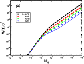
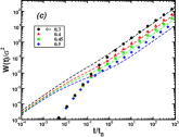
Figure 1: Mean-square displacement $W(t)$ (in units of $\sigma^{2}$) and self-intermediate scattering function $F_{S}(k,t)$ of a hard sphere fluid as a function of the time $t$ (in “molecular units” $t_{0}=\sqrt{M\sigma^{2}/k_{B}T}$) for volume fractions $\phi=0.3,0.4,0.45$ and $0.5$. In all cases, symbols are the results of our MD simulations. The solid lines in (a) and (b) represent, respectively, the solution of Eq. (14) for $W(t)$ and Eq. (22) for $F_{S}(k,t)$ at fixed wave vector $k\sigma=7.18$. The dashed lines in (c) and (d) are the solution of, respectively, Eqs. (13) and (11).

For completeness, in Fig. 1 the solution of the overdamped version of Eq. (14) (see Eq. (13)) using the same overdamped $\Delta\zeta^{*}(t)$ as input has been included. The resulting MSD, represented by the dashed lines, describes the dynamics of the corresponding Brownian liquid whose solution satisfies the short- and long-time limits, i.e., $W(t\to 0)\approx D^{0}t$ and $W(t\to\infty)\approx D_{L}t$, respectively. The comparison between the theoretical curves and the simulation data demonstrates the theoretically predicted long-time dynamic scaling between atomic and colloidal systems in the context of the MSD, as already reported in Ref. atomic3 .

In Fig. 1 the theoretical predictions for $F_{S}(k,t)$ are compared with the corresponding MD results at the same volume fractions. This comparison indicates that the simple approximation in Eq. (22) provides a very good quantitative representation of $F_{S}(k,t)$ at very low volume fractions, although the inaccuracies of the theoretical results for $W(t)$ shown in Fig. 1 manifest themselves in the differences observed, particularly at $\phi=$ 0.5 at intermediate times.

In Fig. 1, the quantitative differences between the solution of the overdamped SCGLE equations (dashed lines) for $F_{S}(k,t)$ and the MD simulation data are illustrated. From this comparison, which complements the information provided in Fig. 1, one can see that the final decay of $F_{S}(k,t)$ is only well captured for $\phi\geq 0.45$. Appreciable differences are observed, however, at shorter times ($t\lesssim t_{0}$), derived from the fact that in atomic systems the relaxation of $F_{S}(k,t)$ in this time regime reflects the early ballistic displacements of the particles, not captured within the overdamped SCGLE theory.

Thus, one can conclude that the overdamped SCGLE equations provide a good representation of the hard-sphere self-ISF at times longer than $t_{0}$, in particular, for volume fractions beyond a threshold value around $\phi\geq 0.45$. Below this threshold value, the overdamped SCGLE theory fails to capture the essentially ballistic decay of the ISF $F_{S}(k,t)$ of atomic liquids. This threshold coincides approximately with the freezing volume fraction, and is actually the same as the crossover volume fraction referred to in Ref. atomic2 , above which the dynamical equivalence between atomic and Brownian liquids is also exhibited by $F_{S}(k,t)$. The fact that this dynamical equivalence holds better when increasing the volume fractions in the metastable regime makes it specially relevant to understand the common phenomenology of colloidal and atomic glass formers, a point that will be addressed elsewhere todoss

IV SCGLE formalism for multicomponent atomic liquids

We now describe the multicomponent extension of the SCGLE theory for atomic liquids. Since such an extension is in reality rather straightforward, we shall not go in any detail through each of the arguments reviewed in the monocomponent case. Instead, we only summarize the resulting set of SCGLE equations that describe the dynamics of a multicomponent atomic liquid and provide two illustrative applications involving the direct comparison with the corresponding MD simulation results. In this section, we also briefly describe the simulation methods employed.

IV.1 Dynamics of multicomponent atomic liquids

Let us consider now an atomic liquid at temperature $T$ inside a volume $V$ and composed of $N$ spherical particles belongin to $\nu$ different species (labeld by the index $i=1,2,...,\nu$). Thus, $N=\sum_{i=1}^{\nu}N_{i}$, where $N_{i}$ is the number of particles of the species $i$, each of one having a mass $M_{i}$ and a diameter $\sigma_{i}$. One can also define the number concentration of species $i$ as $n_{i}=N_{i}/V$. The relevant structural information of these multicomponent atomic liquid is contained in the elements $S_{ij}(k)$ of the $\nu\times\nu$ matrix $S(k)$ of partial static structure factors, whereas the most fundamental dynamical information is contained in the $\nu\times\nu$ matrices $F^{D}(k,t)$ and $F^{D}_{S}(k,t)$, whose elements are the collective and partial self-intermediate scattering functions $F^{D}_{ij}(k,t)$ and $\delta_{ij}F^{D}_{S,i}(k,t)$, respectively.

As explained in detail in Refs. marco2 ; rigo1 , within the SCGLE formalism the time-evolution equations for the matrices $F^{D}(k,t)$ and $F^{D}_{S}(k,t)$, written in Laplace space, reads

$$F^{D}(k,z)=\{zI+k^{2}D\cdot[zI+\lambda(k)\cdot\Delta\hat{\zeta}^{*}(z)]^{-1}$$

$$\cdot S^{-1}(k)\}^{-1}\cdot S(k),$$ (23)

and

$$F^{D}_{S}(k,z)=\{zI+k^{2}D\cdot[zI+\lambda(k)\cdot\Delta\hat{\zeta}^{*}(z)]^{-1}\}^{-1},$$ (24)

where $D$ and $\lambda(k)$ are diagonal matrices given by $D_{ij}\equiv\delta_{ij}D^{0}_{i}$ and $\lambda_{ij}(k)=\delta_{ij}[1+(k/k^{c}_{i})]^{-1}$ and with $D^{0}_{i}$ being the short-time self-diffusion coefficient of species $i$, which depends on the masses $M_{i}$, the temperature, and the size of the particles, in a manner that extends the monocomponent kinetic expression in Eq. (5). The parameter $k^{c}_{i}$ is a empirical cut-off wave-vector written as $k^{c}_{i}=ak^{max}_{i}$, in which $k^{max}_{i}$ is the position of the maximum of $S_{ii}(k)$ and $a>0$ is again the only free parameter, eventually determined by a calibration procedure gabriel .

The $i$th diagonal element $\Delta\zeta^{*}_{i}(z)$ of the matrix $\Delta\hat{\zeta}^{*}(z)$ is the time-dependent friction function of particles of species $i$, and according to Refs. marco2 ; rigo1 is given by

$$\Delta\zeta^{*}_{i}(t)=\frac{D^{0}_{i}}{3(2\pi)^{3}}\int d{\bf k}\ k^{2}[F^{D}_{S}(t)]_{ii}[h\cdot\sqrt{n}\cdot S^{-1}$$

$$\cdot F^{D}(t)\cdot S^{-1}\cdot\sqrt{n}\cdot h]_{ii},$$ (25)

with the elements of the $k$-dependent matrix $h$ given by $h=\sqrt{n}^{-1}\cdot(S-I)\cdot\sqrt{n}^{-1}$, where the elements of the matrix $\sqrt{n}$ are $[\sqrt{n}\ ]_{ij}\equiv\delta_{ij}\sqrt{n_{i}}$, and we have systematically omitted the argument $k$ of the $\nu\times\nu$ matrices $h(k)$, $S(k)$, $F^{D}(k,t)$, and $F^{D}_{S}(k,t)$.

Let us now write the corresponding results for the mean-square displacement, $W(t)$, with its diagonal elements, $W_{i}(t)$, i.e., the MSD of particles of species $i$, given by

$$\tau_{i}^{0}\frac{dW_{i}(t)}{dt}+W_{i}(t)=D_{i}^{0}t-\int_{0}^{\tau}\Delta\zeta^{*}_{i}(t-t^{\prime})W_{i}(t^{\prime})dt^{\prime},$$ (26)

where $\tau_{i}^{0}\equiv M_{i}/\zeta^{0}_{i}$, and with $\zeta^{0}_{i}=k_{B}T/D_{i}^{0}$. Finally, the exponential interpolation functions for the $\nu\times\nu$ matrices $F(k,t)$ and $F_{S}(k,t)$ of a multicomponent atomic liquid can be written as,

$$F(k,t)=F^{D}(k,t)+\{S(k)\cdot\exp[-k^{2}W(t)\cdot S^{-1}(k)]$$

$$-F^{D}(k,t)\}\exp[-t/\tau_{i}^{0}],$$ (27)

and

$$F_{S}(k,t)=F^{D}_{S}(k,t)+\{\exp[-k^{2}W(t)]-$$

$$F_{S}^{D}(k,t)\}\exp[-t/\tau_{i}^{0}].$$ (28)

Eqs. (IV.1)-(IV.1) thus extend to mixtures the SCGLE formalism for an atomic liquid. In what follows, its use will be illustrated with two examples involving binary hard-sphere mixtures. The self-consistent solution of these equations requires the previous determination of the matrix $S(k)$ of partial static factors, which will be obtained using again the Percus-Yevick approximation for multicomponent baxterpymixture liquids and with the corresponding Verlet-Weiss correction ($\phi\to\phi-\phi^{2}/16$) verletweis ; williamsvanmegen . Once $S(k)$ has been determined, we solve Eqs. (IV.1)-(25) to obtain the matrices $\Delta\zeta^{*}(t)$, $F^{D}(k,t)$, and $F^{D}_{S}(k,t)$, which describe the dynamics of the multicomponent atomic liquid in the diffusive or overdamped regime. We then use these results in Eqs. (26)-(IV.1) to determine the MSD, $W(t)$, and the ISFs $F(k,t)$ and $F_{S}(k,t)$, which include the correct short-time ballistic regime.

IV.2 Molecular dynamic simulations

As said in the introduction, to test this SCGLE theory of the dynamics of atomic mixtures we have carried out event-driven molecular dynamics simulations in the context of two illustrative applications: a polydisperse HS liquid, modeled as a moderately size-asymmetric binary HS mixture, and a genuine, highly size-asymmetric binary HS mixture. Let us now briefly describe the simulation methods employed in each of these applications.

To simulate a polydisperse monocomponent HS liquid we followed the methodology explained in Ref. gabriel , using event-driven MD simulations. The simulations were carried out with $N=1000$ particles in a volume $V$. The diameters of these particles are uniformly distributed between $\overline{\sigma}(1-w/2)$ and $\overline{\sigma}(1+w/2)$, with $\overline{\sigma}$ being the average particle diameter. We have considered the case $w=0.3$, which corresponds to a polydispersity $s_{\sigma}=w/\sqrt{12}=0.0866$. We have assumed that all particles have the same mass $M$ and the results are displayed in reduced units, therefore, $\overline{\sigma}$ and $\overline{\sigma}\sqrt{M/k_{B}T}$ are used as units of length and time, respectively. To improve the statistics and reduce the uncertainties, every correlation function is obtained over the average of 10 independent realizations for each volume fraction considered. The same protocol was employed to simulate the particular case of a monodisperse HS liquid ($w=0$). In general, the effect of polydispersity on the dynamic properties $W(t)$ and $F_{S}(k,t)$ is not as dramatic as in the structure zaccareli , and the differences are even less noticeable in the stable liquid regime illustrated in Fig. 1,

In the case of highly asymmetric binary mixtures, we have carried out event-driven MD simulations for a HS binary system with asymmetry parameter $\delta\equiv\sigma_{s}/\sigma_{b}=0.2$. Here the labels s and b corresponds, respectively, to small and big. Thus, we have simulated a system of $N(=N_{b}+N_{s})$ particles, consisting in $N_{b}$ big particles and $N_{s}$ small particles, in a volume V. More specifically, we have considered three different state points in the control parameter space of the system spanned by the pair ($\phi_{b},\phi_{s}$), where $\phi_{i}=\pi n_{i}\sigma_{i}^{3}/6$ and $n_{i}=N_{i}/N$ ($i=b,s$). Given $N_{b}$, the size of the cubic simulation box was adjusted in order to control $\phi_{b}$. Then, $N_{s}$ was adjusted to control $\phi_{s}$ (see Ref. todoss ). The specific simulated state points were I$=(0.45,0.05)$, with $N_{b}=200$ and $N_{s}=2778$; II$=(0.45,0.2)$, with $N_{b}=150$ and $N_{s}=8333$; and III$=(0.6,0.05)$, with $N_{b}=200$ and $N_{s}=2083$. For the state points I and III, $10$ realizations of the system were performed, i.e., runs with 10 different seeds have been used to explore the available phase space and to improve the statistics. For the state point II, 5 different seeds have been considered. In these simulations, the unit of length is defined by the diameter of the large particles, $\sigma_{b}$, and the unit of mass is defined as the mass of the big particles, $M_{b}$. The mass densities, $\rho^{M}_{i}\equiv M_{i}/v_{i}$ ($v_{i}=4\pi\sigma^{3}_{i}/3,i=s,b$), are set equal to define the mass of the small particles. Setting $k_{B}=1$, the unit of time is defined from the equipartition theorem $\langle v_{b}^{2}\rangle=3k_{B}T/M_{b}$. Periodic boundary conditions were employed in all directions. It is also worth to stress that, for the points I and II, we have used a waiting time $t_{w}=10^{3}$, while for III we let $t_{w}=10^{4}$, in order to avoid aging effects (see Ref. todoss ). Finally, it should be mentioned that in order to generate non-overlapping initial configurations, a soft-core standard molecular dynamics with a repulsive short-range potential and decreasing temperature was implemented vargas . This soft-core MD starts from a completely random initial configuration.

IV.3 Polydisperse hard-sphere atomic liquid

Let us now proceed to solve the SCGLE Eqs. (IV.1)–(IV.1) for the first of the two examples just described, namely, a polydisperse HS liquid with uniform size distribution and polydispersity $s_{\sigma}=0.0866$. We can model this distribution with its discretize version by partitioning the interval $\overline{\sigma}(1-w/2)\leq\sigma\leq\overline{\sigma}(1+w/2)$ in $\nu$ equally sized bins, and treat the polydisperse liquid as a $\nu$-component mixture. To compare with the simulations we then compute the total properties, such as $W(t)\equiv\sum_{i=1}^{\nu}x_{i}W_{i}(t)$, $F(k;t)=\sum_{i,j=1}^{\nu}\sqrt{x_{i}x_{j}}F_{ij}(k,t)$, and $F_{S}(k,t)\equiv\sum_{i=1}^{\nu}x_{i}F^{S}_{i}(t)$, where $W_{i}(t)$, $F_{ij}(k,t)$, and $F^{S}_{i}(t)$ are the partial MSD, collective ISFs, and self ISFs of the mixture, and where $x_{i}=n_{i}/\sum_{i=1}^{\nu}n_{i}$.

To solve Eqs. (IV.1)-(IV.1) we need first to determine its static input, i.e., the partial static structure factors, but as said above, for our HS system these will be provided by the multicomponent Percus-Yevick approximation with its Verlet-Weiss correction baxterpymixture ; verletweis ; williamsvanmegen . We also need to previously determine the short-time self-diffusion coefficients $D^{0}_{i}$ ($i=1,2...\nu$). Unfortunately, the random-flight arguments involved in the derivation of the monocomponent kinetic-theoretical expression in Eq. 5 are not easily generalized to the case of an arbitrary $\nu$-component atomic liquid. Thus, if we do not wish to treat these as free adjustable parameters, we must resort to additional approximations or simplifications, as we do in the present application.

Thus, to model the simulated HS polydisperse liquid, let us use the approach just described in its simplest form, i.e., by considering an equimolar HS binary mixture, with components having number concentrations $n_{1}=n_{2}=n_{t}/2$ and particle diameters $\sigma_{1}=\overline{\sigma}(1-\epsilon)$ and $\sigma_{2}=\overline{\sigma}(1+\epsilon)$, with $\epsilon=0.0866$ chosen such that the mean diameter, $\bar{\sigma}$, and mean-square diameter $\bar{\sigma^{2}}$ (and hence, the polydispersity), is the same as that of the simulated system. Furthermore, given the small asymmetry between the constituent particles ($\delta\approx 0.84$), it is reasonable to approximate the short-time self-diffusion coefficients $D^{0}_{1}$ and $D^{0}_{2}$ as $D^{0}_{1}=D^{0}_{2}=D^{0}_{eff}$ where $D^{0}_{eff}$ is the short-time self-diffusion coefficient of an effective monodisperse system with concentration $n_{t}$ and diameter $\bar{\sigma}$, given by (see Eq. 5)

$$D^{0}_{eff}\equiv\frac{3}{8}\left(\frac{k_{B}T}{\pi M}\right)^{1/2}\frac{1}{n_{t}\bar{\sigma}^{2}}.$$ (29)

As it is shown in what follows, this proposal allows us to provide a good representation of the referred dynamical properties of the simulated polydisperse fluid.

Figure 2: (a) Mean-square displacement $W(t)$ and (b) self-ISF, $F_{S}(k,t;\phi)$, at fixed $k\bar{\sigma}=7{.}1$, as a function of time $t$ (in “molecular” units $t_{0}\equiv\bar{\sigma}\sqrt{M/k_{B}T}$) for the polydisperse hard-sphere atomic liquid (polydisersity = 8.66 %) at the indicated volume fractions. In both figures, solid symbols represents the MD simulation data and the solid lines are the predictions of the SCGLE formalism for atomic liquids.

In Fig. 2 we show the theoretical predictions for $W(t)$ and $F_{S}(k,t)$ compared against the corresponding MD simulation results for a set of volume fractions. This figure illustrates how, using the overdamped friction functions $\Delta\zeta^{*}_{i}(t)$ in the time-evolution equations for $W_{i}(t)$ (Eqs. (26)) and assuming $D^{0}_{1}=D^{0}_{2}=D^{0}_{eff}$, an effective MSD (solid lines) is generated, which nicely describes the ballistic regime, although some quantitative differences appears at long-times. Such deviations, however, should be expected considering the calibration procedure employed to fix the only phenomenological parameter of the SCGLE theory (the cutoff wave-vector $k^{c}_{i}$) as $k^{c}_{i}=ak^{max}_{i}$, with $a=1.119$. This value was chosen in order to get the best overall fit of the theory with the simulation data for the so-called $\alpha$-relaxation time $\tau^{(\alpha)}$, defined by $F_{S}(k\bar{\sigma}=7.1,t=\tau^{(\alpha)})=e^{-1}$. For this reason, the overall long-time agreement with the simulation results of the predicted $F_{S}(k,t)$ (see Fig. 2) is in general better than that of $W(t)$. Similar to the MSD, one observes that for volume fractions smaller than 0.5, the quality of the agreement at short and long times is better than that seen in the metastable regime, $\phi\gtrsim 0.5$, where there are some quantitative differences. Thus, in spite of the use of the approximate effective diffusion coefficient in Eq. 29, the results show a nice agreement between simulation and theory.

IV.4 Highly size-asymmetric binary mixture

The previous example illustrates a simple manner to apply the SCGLE theory of atomic mixtures to represent the dynamical properties of a polydisperse fluid. The small degree of polydispersity allowed us to use the approximation $D^{0}_{1}=D^{0}_{2}=D^{0}_{eff}$. Let us now turn our attention to the case of highly asymmetric HS binary mixtures, illustrated with the simulated mixture with size asymmetry $\delta=0.2$ (and mass asymmetry $M_{s}/M_{b}=\delta^{3}=0.008$). The theoretical procedure is exactly the same, except that now we need to keep track of the partial dynamic properties $W_{i}(t)$, $F_{ij}(k,t)$, and $F^{S}_{i}(t)$, and the size- and mass-asymmetries are much larger. This forces to consider more accurate expressions for the short-time diffusion coefficients $D^{0}_{1}$ and $D^{0}_{2}$ provided by kinetic theory, namely mcquarrie ,

$$D^{0}_{b}=\frac{3}{2}\left(\dfrac{k_{B}T}{\pi M_{b}}\right)^{1/2}\left[\dfrac{1}{4\sigma_{b}^{2}n_{b}+(\sigma_{b}+\sigma_{s})^{2}n_{s}}\right]$$ (30)

$$D^{0}_{s}=\frac{3}{2}\left(\dfrac{k_{B}T}{\pi M_{s}}\right)^{1/2}\left[\dfrac{1}{(\sigma_{b}+\sigma_{s})^{2}n_{b}+4\sigma_{s}^{2}n_{s}}\right],$$ (31)

which contains the monocomponent expression in Eq. (5) as a particular case.

In practice, however, since the big particles are far more massive than the small particles, in determining the self-diffusion coefficient of the large spheres, we simply assume that the most representative collisions contributing to $D^{0}_{b}$ are those among big particles, and thus, we may approximate such coeficient by (see Eq. (5))

$$D^{0}_{b}\equiv\frac{3}{8}\left(\frac{k_{B}T}{\pi M_{b}}\right)^{1/2}\frac{1}{n_{b}\sigma^{2}_{b}}.$$ (32)

For the small particles, however, we do consider both types of collisions, i.e., those involving only small particles and those among small and large ones, so that

$$\dfrac{D^{0}_{s}}{D^{0}_{b}}=4\left(\dfrac{M_{b}}{M_{s}}\right)^{1/2}\left[\dfrac{\sigma_{b}^{2}n_{b}}{(\sigma_{b}+\sigma_{s})^{2}n_{b}+4\sigma_{s}^{2}n_{s}}\right].$$ (33)

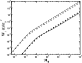
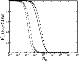
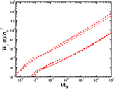
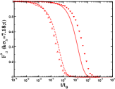
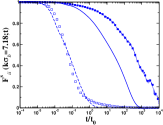
Figure 3: Theoretical (solid and dotted lines) and simulation (solid and open symbols) results for the MSDs, $W_{i}(t)$, and ISFs $F^{s}_{i}(k=7.18;t)$ of a highly asymmetric ($\delta=0.2$) binary mixture of HS, for the three volume fractions, in the control parameter space $(\phi_{b},\phi_{s})$. (a) and (b) Corresponds to the point I$=(0.45,0.05)$. (c) and (d) Corresponds to II$=(0.45,0.2)$. (e) and (f) Corresponds to III$=(0.60,0.05)$. In all cases, solid symbols ($\CIRCLE$,$\blacktriangle$, $\blacksquare$) and solid lines corresponds to the dynamical properties of big particles, whereas empty symbols ($\Circle$, $\bigtriangleup$, $\square$) and dashed lines accounts for small particles.

To test the accuracy of the resulting approximate theory, we have solved Eqs. (26)-(IV.1) with Eqs. (32) and (33) for the MSDs, $W_{i}(t)$, and self-ISFs, $F^{S}_{i}(t)$, of the highly asymmetric binary HS mixture ($\delta=0.2$) for three aforementioned state points in the high-concentration region of the control parameter space $(\phi_{b},\phi_{s})$, namely, I$=(0.45,0.05)$, II$=(0.45,0.2)$, and III$=(0.60,0.05)$. The corresponding predictions are compared in Fig. 3 with their simulation counterparts. The first bird-eye conclusion of this comparison is that the theory provides quite a reasonable representation of the simulation results, considering its approximate nature and the simplicity of its underlying approximations and simplifications.

More quantitatively, we notice that the theoretical results exhibit the correct short- and long-time behavior of $W_{i}(t)$, including the disparate time-scales of the dynamics of $W_{b}(t)$ and $W_{s}(t)$ when plotted as a function of the scaled time $t_{m}$ (defined in units of $\sigma_{b}$ and $M_{b}$). This time-scale difference originates in the huge mass ratio $M_{s}/M_{b}=\delta^{3}=0.008$. This can be seen through the short-time (ballistic) solution of Eq. (26), $<(\Delta\mathbf{r}_{i}(t))^{2}>\approx[3k_{B}T/M_{i}]t^{2}$ which, expressed in terms of $W_{i}(t)=<(\Delta\mathbf{r}_{i}(t))^{2}>/6$, reads

$$\dfrac{W_{i}(t_{m})}{\sigma_{b}^{2}}=\dfrac{1}{2}\left[\dfrac{M_{b}}{M_{i}}\right](t_{m})^{2},$$ (34)

where $t_{m}\equiv t/t^{0}_{b}$ and $t^{0}_{b}=\sigma_{b}\sqrt{M_{b}/k_{B}T}$. The ratio $[M_{b}/M_{i}]$ is unity for the big particles ($i=b$) and is 0.008 for the small particles ($i=s$), thus explaining the aforementioned time-scale difference.

Figs. 3-3, 3-3 and 3-3 correspond, respectively, to the points I, II and III. These figures illustrate the effect on the dynamics of the system upon variations in the two control parameters $\phi_{b}$ and $\phi_{s}$. For instance, regarding the dynamics of the system at the state point I$=(\phi_{b}=0.45,\phi_{s}=0.05)$, one notices that, besides the aforementioned time-scale difference in the MSDs of both species observed in Fig. 3, the SCGLE results for the ISFs of each species in Fig. 3 (solid and dashed lines) also reveals a noticeable difference between the characteristic decay times of the ISFs of each species, although the one-step relaxation pattern of each correlator is rather similar. The differences in the decay times are described by the $\alpha$-relaxation times, $\tau^{(\alpha)}_{i}$ ($i=b,s$), defined here as $F^{S}_{i}(k\sigma_{b}=7.18;\tau^{(\alpha)}_{i})=1/e$. These features are consistent with the results obtained from MD simulations (solid and open symbols).

Upon increasing $\phi_{s}$ from 0.05 to 0.2 we go from state point I to state point II$=(0.45,0.2)$, and in Figs. 3 and 3 we observe that the mobility of both species decrease. In addition, the crossover from the ballistic to the diffusive regime occurs at shorter times compared with the situation illustrated at I, and the difference between the corresponding $\alpha$-relaxation times become larger. The simulation results nicely confirm these trends.

A more interesting behavior is observed when we move from state point I to state point III$=(0.6,0.05)$, this time by fixing $\phi_{s}=0.05$ and increasing $\phi_{b}$ from 0.45 to 0.6, above the glass transition threshold $\phi^{(g)}\approx 0.582$ of the monodisperse HS fluid. As illustrated in Figs. 3-3, in addition to the different time-scales of $W_{b}(t)$ and $W_{s}(t)$ derived from the disparate mass difference, a further enhancement of this difference is now quite visible at long times, suggesting a strong disparity in the structural relaxation of the two species. For instance, a large disparity in the mobility of each species, measured by the ratio $W_{b}(t_{m}=10^{3})/W_{s}(t_{m}=10^{3})\sim 10^{-3}$, is observed. Notice also the emergence of an incipient plateau in the MSD of the large particles, which is absent in the MSD of the small ones.

This long-time dynamic asymmetry is also observed in the ISFs of each species, which displays different relaxation patterns, characterized by a faster relaxation mechanism for the small particles and a far slower relaxation of the large particles. Except for quantitative details, mostly manifested in $F^{S}_{bb}(k,t)$, the comparison with the simulation data demonstrates that these theoretical predictions capture the essential phenomenology of the simulation results.

V Concluding remarks

In this paper we have proposed and tested an approximate but quantitative theoretical approach for the description of the dynamics of fully equilibrated atomic liquid mixtures. Such framework was built on the exact time-evolution equations for the long-time dynamics of an atomic liquid, previously developed in Refs. atomic1 ; atomic2 ; atomic3 , which were complemented by a set of well-defined approximations, including a Gaussian-like approximation that incorporates the correct ballistic short-time limit. The predictive accuracy of the resulting theoretical tool was confirmed with the assistance of pertinent molecular dynamics simulations. The general conclusion drawn from these numerical tests indicate a remarkable degree of reliability of the present SCGLE theory. Although its quantitative accuracy could be improved in several manners, this was not the primary interest of the present work. Here we focused, instead, in illustrating the systematic use of our theory in two representative and concrete examples. The first involved a simple but polydisperse HS liquid and the second a genuine and highly-asymmetric binary mixture of hard spheres.

In both cases we expect that the present approximate theory will evolve into a useful theoretical tool to model the properties of experimentally-relevant atomic liquid mixtures, such as molten salts and metallic alloys. This unification of the physics of colloidal and atomic liquids clearly creates an opportunity to systematically transfer much of the knowledge generated in the field of colloids to the understanding of complex atomic liquid mixtures and vice versa. For instance, both examples discussed here actually derive from two separate projects involving model colloidal HS liquids, whose properties could in practice be more easily simulated using event-driven molecular dynamics, rather than the more natural Brownian dynamics simulations. In the first example, since hard-sphere colloids are usually polydisperse, theoretically describing polydispersity with the SCGLE theory and then testing the results with MD simulations is now a natural and handy modeling protocol, as discussed in more detail elsewhere patygabriel . The same protocol is being followed in modeling the dynamics of genuine HS colloidal mixtures with large size asymmetry, and discussed in more detail in separate work todoss .

Finally, another particularly relevant opportunity is represented by the possibility of connecting the advances in our understanding of the formation of colloidal glasses and gels with the technologically relevant need to understand the formation of amorphous solids by the cooling of complex glass- and gel-forming atomic liquids. Although this more ambitious project requires the development of the non-equilibrium version of the present SCGLE theory of equilibrium atomic liquids, the present work paves the way for such developments.

VI Acknowledgments

This work was supported by the Consejo Nacional de Ciencia y Tecnología (CONACYT, México) through grants Nos. 242364, 182132, 237425, 358254, and FC-2015-2/1155, and by the Universidad de Guanajuato (through the Convocatoria Institucional para el Fortalecimiento de la Excelencia Académica 2015). L.F.E.A. and R.C.P. acknowledge financial support from Secretaría de Educación Pública (SEP, México) through Postdoctoral fellowship, PRODEP. P.M.M. and M.M.N. acknowledge the support of Secretaría de Educación Pública through Postdoctoral fellowship, PRODEP. L.F.E.A also acknowledge financial support from the German Academic Exchange Service (DAAD) through the DLR-DAAD programme under grant No. 212. R. C. P. also acknowledges the financial support provided by the Marcos Moshinsky fellowship 2013 - 214 and the Alexander von Humboldt Foundation during his stay at the University of Düsseldorf in summer 2016. The authors acknowledge Thomas Voigtmann for interesting discussions.

References

- (1) P. N. Pusey in Liquids, Freezing and Glass Transition, edited by J. P. Hansen, D. Levesque, and J. Zinn-Justin (Elsevier, Amsterdam, 1991), Chap. 10.
- (2) I. M. de Schepper, E. G. D. Cohen, P. N. Pusey, and H. N. W. Lekkerkerker, J. Phys. Condens. Matter. 1, 6503 (1989).
- (3) P. N. Pusey, H. N. W. Lekkerkerker, E. G. D. Cohen, and I. M. de Schepper, Physica A 164, 12 (1990).
- (4) H. Löwen, J. P. Hansen, and J. N. Roux, Phys. Rev. A 44, 1169 (1991).
- (5) G. Szamel and E. Flenner, Europhys. Lett., 67, 779 (2004).
- (6) A. M. Puertas, J. Phys.: Condens. Matter 22: 104121 (2010).
- (7) G. Szamel and H. Löwen, Phys. Rev. A 44, 8215 (1991).
- (8) L. López-Flores, P. Mendoza-Méndez, L. E. Sánchez-Díaz, L. L. Yeomans-Reyna, A. Vizcarra-Rendón, G. Pérez-Ángel, M. Chávez-Páez, and M. Medina-Noyola, Europhys. Lett. 99, 46001 (2012).
- (9) M. Medina-Noyola and J. L. del Río-Correa, Physica 146A, 483 (1987).
- (10) M. Medina-Noyola, Faraday Discuss. Chem. Soc. 83, 21 (1987).
- (11) P. Mendoza-Méndez, L. López-Flores, A. Vizcarra-Rendón, L. E. Sánchez-Díaz, and M. Medina-Noyola, Physica A 394, 1 (2014).
- (12) L. López-Flores, L. L. Yeomans-Reyna, M. Chávez-Páez, and M. Medina-Noyola, J. Phys.: Condens. Matter 24, 375107 (2012).
- (13) L. López-Flores, H. Ruíz-Estrada, M. Chávez-Páez, and M. Medina-Noyola, Phys. Rev. E 88, 042301 (2013).
- (14) L. Yeomans-Reyna and M. Medina-Noyola, Phys. Rev. E 64, 066114 (2001).
- (15) L. Yeomans-Reyna, H. Acuña-Campa, F. Guevara-Rodríguez, and M. Medina-Noyola, Phys. Rev. E 67, 021108 (2003).
- (16) L. Yeomans-Reyna et al., Phys. Rev. E 76, 041504 (2007).
- (17) R. Juárez-Maldonado et al., Phys. Rev. E 76, 062502 (2007).
- (18) D.A. McQuarrie, Statistical Mechanics, Harper and Row, N.Y. (1975).
- (19) M. A. Chávez-Rojo and M. Medina-Noyola, Phys. Rev. E 72, 031107 (2005); ibid 76: 039902 (2007).
- (20) R. Juárez-Maldonado and M. Medina-Noyola, Phys. Rev. E 77, 051503 (2008).
- (21) W. Götze, in Liquids, Freezing and Glass Transition, edited by J. P. Hansen, D. Levesque, and J. Zinn-Justin (North-Holland, Amsterdam, 1991).
- (22) W. Götze and L. Sjögren, Rep. Prog. Phys. 55, 241 (1992).
- (23) J. Bosse and J. S. Thakur, Phys. Rev. Lett. 59, 998 (1987).
- (24) J. L. Barrat and A. Latz, J. Phys. Condens. Matter 2, 4289 (1990).
- (25) G. Nägele, J. Bergenholtz and J. K. G. Dhont, J. Chem. Phys. 110, 7037 (1999)
- (26) Angell C. A., Ngai K. L., McKenna G. B., McMillan P. F. and Martin S. F., J. Appl. Phys. 88 3113 (2000).
- (27) P. E. Ramírez-González and M. Medina-Noyola, Phys. Rev. E 82, 061503 (2010).
- (28) L. E. Sánchez-Díaz, P. E. Ramírez-González, and M. Medina-Noyola, Phys. Rev. E 87, 052306 (2013).
- (29) J. M. Olais-Govea, L. López-Flores, and M. Medina-Noyola, J. Chem Phys. 143, 174505 (2015).
- (30) G. E. Uhlenbeck and L. S. Ornstein, Phys. Rev. 36, 823 (1930).
- (31) L. Yeomans-Reyna and M. Medina-Noyola, Phys. Rev. E 62, 3382 (2000).
- (32) G. Pérez-Ángel, L. E. Sánchez-Díaz, P. E. Ramírez-González, R. Juárez-Maldonado, A. Vizcarra-Rendón, and M. Medina-Noyola, Phys. Rev. E 83, 060501(R) (2011)
- (33) J. L. Boon and S. Yip, Molecular Hydrodynamics (Dover Publications Inc. N. Y., 1980).
- (34) J. K. Percus and G. J. Yevick, Phys. Rev. 110, 1 (1957).
- (35) L. Verlet and J.-J. Weis, Phys. Rev. A 5 939 (1972).
- (36) L.F. Elizondo-Aguilera, E. Lázaro-Lázro, J.A. Perera-Burgos, G. Pérez-Ángel, M. Medina-Noyola and R. Castañeda-Priego , manuscript in preparation (2017).
- (37) R. J. Baxter, J. Chem. Phys. 52, 4559 (1970).
- (38) S. R. Williams and W. van Megen, Phys. Rev. E 64, 041502 (2001).
- (39) E. Zaccarelli, C. Valeriani, E. Sanz, W. C. K. Poon, M. E. Cates, and P. N. Pusey, Phys. Rev. Lett. 103, 135704 (2009).
- (40) M. C. Vargas and G. Pérez-Ángel, Phys. Rev. E. 87, 042313 (2013).
- (41) P. Mendoza-Méndez, E. Lázaro-Lázaro, L. E. Sánchez-Díaz, P. E. Ramírez-González, G. Pérez-Ángel, and M. Medina-Noyola, Manuscript in preparation (2017).