Refinement of the timing-based estimator of pulsar magnetic fields

Abstract

Numerical simulations of realistic non-vacuum magnetospheres of isolated neutron stars have shown that pulsar spin-down luminosities depend weakly on the magnetic obliquity $\alpha$. In particular, $L\propto B^{2}(1+\sin^{2}\alpha)$, where $B$ is the magnetic field strength at the star surface. Being the most accurate expression to date, this result provides the opportunity to estimate $B$ for a given radiopulsar with quite a high accuracy. In the current work, we present a refinement of the classical ‘magneto-dipolar’ formula for pulsar magnetic fields $B_{\rm md}=(3.2\times 10^{19}\mbox{ G})\sqrt{P\dot{P}}$, where $P$ is the neutron star spin period. The new, robust timing-based estimator is introduced as $\log B=\log B_{\rm md}+\Delta_{\rm B}(M,\alpha)$, where the correction $\Delta_{\rm B}$ depends on the equation of state (EOS) of dense matter, the individual pulsar obliquity $\alpha$ and the mass $M$. Adopting state-of-the-art statistics for $M$ and $\alpha$ we calculate the distributions of $\Delta_{\rm B}$ for a representative subset of 22 EOSs that do not contradict observations. It has been found that $\Delta_{\rm B}$ is distributed nearly normally, with the average in the range $-0.5$ to $-0.25$ dex and standard deviation $\sigma[\Delta_{\rm B}]\approx$ 0.06 to 0.09 dex, depending on the adopted EOS. The latter quantity represents a formal uncertainty of the corrected estimation of $\log B$ because $\Delta_{\rm B}$ is weakly correlated with $\log B_{\rm md}$. At the same time, if it is assumed that every considered EOS has the same chance of occurring in nature, then another, more generalized, estimator $B^{*}\approx 3B_{\rm md}/7$ can be introduced providing an unbiased value of the pulsar surface magnetic field with $\sim$30 per cent uncertainty with 68 per cent confidence. Finally, we discuss the possible impact of pulsar timing irregularities on the timing-based estimation of $B$ and review the astrophysical applications of the obtained results.

1 Introduction

Radiopulsars are strongly magnetized neutron stars (NSs). The large-scale magnetic field, originating in their crusts (and, probably, in the cores), plays a crucial role in many phenomena related to these compact remnants of stellar evolution. However, only a few dozen nearly direct measurements of NS magnetic fields have been made so far – typically for high-energy sources in binary systems. These measurements are based on accretion and/or emission physics, such as the detection of a cyclotron resonant scattering feature in the X-ray spectra of a compact object (see for instance Chashkina & Popov, 2012; Tiengo et al., 2013; Revnivtsev & Mereghetti, 2015; Borghese et al., 2015, and references therein).

The magnetic fields of isolated radiopulsars can be routinely inferred from their timing. Indeed, pulsar rotational histories are to a large extent driven by the properties of their magnetospheres – through the charged particle winds and the surface currents acting on the star. On the other hand, the evolution of the pulsar spin period P(t) can be directly traced because of the anisotropy of the radio emission.

The topology of the magnetic field of an isolated NS is typically assumed to be purely (or predominantly) dipolar, because higher-order multipoles decrease rapidly with distance from the star. In this case, the braking torque component aligned with the star spin axis can be calculated as

$$N=-\mu^{2}\left(\dfrac{\Omega}{c}\right)^{3}f(\alpha),$$ (1)

where $\mu$ is the dipolar magnetic moment, $\Omega=2\pi/P$ is the spin frequency, $c$ is the speed of light, while $f(\alpha)$ is the dimensionless function of the angle $\alpha$ between the magnetic and spin axes. The cubic dependence of $N$ on the inverse light-cylinder radius $r_{\rm{}_{LC}}=c/\Omega$ (the natural size of the magnetosphere) and the quadratic dependence on the moment $\mu$ probably reflects the dipolar structure of the field and is common in most theories of pulsar spin-down. In contrast, the particular form of $f(\alpha)$ is highly dependent on the adopted physics and can be generically written as

$$f(\alpha)=x_{\perp}\sin^{2}\alpha+x_{\parallel}\cos^{2}\alpha,$$ (2)

where $x_{\perp}$ and $x_{\parallel}$ are the coefficients describing the losses of rotational energy by perfectly orthogonal and aligned rotators, respectively.

For a spherical NS with moment of inertia $I$ and radius $R$, equation (1) can be rewritten as the spin-down law

$$P\dfrac{{\rm d}P}{{\rm d}t}=\dfrac{4\pi^{2}R^{6}}{Ic^{3}}B^{2}f(\alpha),$$ (3)

where $B=\mu/R^{3}$ is the field strength at the magnetic equator. This law explicitly defines $B$ as a function of period $P$ and its derivative $\dot{P}$, which is the basis of the timing-based estimation of the magnetic field. Of course, the precise calculation of $B$ requires the radius $R$, the moment of inertia $I$ and the magnetic angle $\alpha$ of a given pulsar to be known as well. The latter quantity is the most crucial – indeed, if $x_{\perp}\gg x_{\parallel}$ or vice versa, then even a moderate uncertainty in $\alpha$ will lead to a significant error in the derived value of $B$. Moreover, when $\alpha$ is completely unknown, only a lower limit of the surface field can be obtained. On the other hand, the radii and moments of inertia are expected to be relatively narrowly distributed over the pulsar population, mostly owing to the plateau in the mass–radius relationship predicted by realistic equations of state (see Fig. 3). Thus, a confident knowledge of $f(\alpha)$ seems to be the key component in the calculation of pulsar magnetic fields

Many models of radiopulsar spin-down (in terms of $f(\alpha)$ parametrization) have been discussed in the literature for the last half-century (see Beskin et al. (2013) for a review). For instance, the classical but naive model of vacuum ‘magnetodipolar’ losses owing to the radiation-reaction torque assumes $x_{\perp}\in 0.3-1.3$ and $x_{\parallel}\equiv 0$ (Deutsch, 1955; Davis & Goldstein, 1970; Good & Ng, 1985; Melatos, 2000). The most frequently used version of this model, with $x_{\perp}=2/3$, $\alpha=90\degr$, moment of inertia $I=I_{0}=10^{45}$ g cm² and radius $R=R_{0}=10$ km, provides the ‘standard’ widely used equation for the pulsar magnetic field (e.g. Manchester & Taylor, 1977; Shapiro & Teukolsky, 1983):

$$B_{\rm md}(P,\dot{P})=\sqrt{\dfrac{3I_{0}c^{3}}{8\pi^{2}R_{0}^{6}}\cdot P\dot{P}}=3.2\times 10^{19}\sqrt{P\dot{P}}\mbox{ G}$$ (4)

Even if one disregards the fact that equation (4) is based on unrealistic assumptions (namely, a vacuum NS magnetosphere and common values of $I$ and $R$ for all pulsars), the obliquity $\alpha=90\degr$ assumed in $B_{\rm md}$ makes its value formally only a lower limit of the NS surface field strength.

The ‘magneto-dipolar’ losses vanish for a perfectly aligned rotator ($\alpha=0\degr$). On the other hand, earlier investigations of axisymmetric plasma-filled magnetospheres have shown that a NS with zero obliquity still efficiently loses its rotational energy (e.g Goldreich & Julian, 1969; Michel, 1973; Ruderman & Sutherland, 1975). Later, Beskin et al. (1993) obtained a general analytic solution for a non-vacuum NS magnetosphere with arbitrary $\alpha$, adopting a number of reasonable simplifications. They found that $x_{\parallel}\approx x_{\perp}(\Omega R/c)^{-1}$. In this case, the first term of (2) appears to be almost suppressed because $\Omega R/c\sim 10^{-4}$ to $10^{-2}$ for actual pulsars (see also Beskin & Nokhrina, 2007). Hence, even in this more physically justified model, the magnetic field estimation (derived from the corresponding spin-down law $P\dot{P}\propto\Omega^{3}\cos^{2}\alpha$) still crucially depends on the obliquity $\alpha$.

It has been proposed in the last decade, however, that the observed spin-down of actual pulsars can be satisfactorily explained by assuming that the two terms of $f(\alpha)$ contribute comparably to the braking torque; that is, $x_{\perp}\sim x_{\parallel}$ (Xu & Qiao, 2001; Contopoulos & Spitkovsky, 2006; Barsukov et al., 2009; Barsukov & Tsygan, 2010; Kou & Tong, 2015; Kou et al., 2016; Ou et al., 2016). If this is the case, it can be expected that the spindown rate ${\rm d}P/{\rm d}t$ depends relatively weakly on the obliquity $\alpha$, thus eliminating the problem of ‘uncertain magnetic field estimation’ described above.

This proposition has been well supported by the results from direct three-dimensional magnetohydrodynamical (MHD) and particle-in-cell numerical simulations of oblique pulsar magnetospheres performed by a number of groups (Spitkovsky, 2006; Kalapotharakos & Contopoulos, 2009; Pétri, 2012; Tchekhovskoy et al., 2013; Philippov et al., 2014). It has been found that $f(\alpha)$ can be approximated by the simple analytic formula

$$f(\alpha)=k_{0}+k_{1}\sin^{2}\alpha,$$ (5)

where both $k_{0}$ and $k_{1}$ are close to unity and constant to within the terms proportional to $(\Omega R/c)^{2}$. In terms of equation (2), it means that $x_{\perp}=k_{0}+k_{1}$ and $x_{\parallel}=k_{0}$ respectively. Being the most accurate solution obtained so far, this improved and quite simple form of $f(\alpha)$ provides a way to measure the surface magnetic field of observed isolated pulsars with a relatively high precision, even when $\alpha$ remains unknown.

The overall aim of our research is to derive the correction for the classical estimator $B_{\rm md}$ on the basis of the state-of-the-art understanding of the properties and spin-down physics of isolated NSs. We start from the spin-down torque (1) assuming (5) as initially derived by Spitkovsky (2006) and developed by Tchekhovskoy et al. (2013) and Philippov et al. (2014). Taking into account the existing observational constraints on isolated NS masses and obliquity distributions and considering a representative subset of more than 20 realistic equations of state, we estimate the realistic uncertainties that can be achieved in the measurement of a pulsar magnetic field.

We note that after this work was finished, Nikitina & Malov (2016) published the results of their re-calculation of $B$ for 376 pulsars using their original values of magnetic angles. However, they used the classical ‘magneto-dipolar’ spin-down law and did not take into account either the scatter of masses over the NS population or a realistic equation of state.

The paper is organized as follows. In Section 2 we provide the general equations for the magnetic field calculations and introduce the refined formula. In Section 3 the masses and obliquities of isolated NSs are discussed and a list of realistic equations of state is described. These data are used in Section 4 to calculate the uncertainty of the proposed estimator. In Section 5 the possible impact of the pulsar timing irregularities on the magnetic field estimations, as well as applications of our results, are discussed. In Section 6 a summary of the work is provided and conclusions are enumerated. Finally, in Appendix A, the parameters of a NS with various equations of state are given and relevant calculations are presented.

2 The timing-based magnetic field estimator

Hereafter, we assume that a radiopulsar with magnetic field strength $B$ at the equator, spin period $P$ and obliquity $\alpha$ loses its rotational energy according to the equation

$$P\dot{P}=\dfrac{4\pi^{2}R^{6}}{Ic^{3}}B^{2}(1+1.4\sin^{2}\alpha),$$ (6)

which was derived numerically for a spherical oblique rotator with a plasma-filled magnetosphere by Philippov et al. (2014) and is nothing more than a restatement of the general equation (3) with $f(\alpha)$ in the form (5) with $k_{0}=1.0$ and $k_{1}=1.4$. Extracting the value of the magnetic field gives

$$B=\sqrt{\dfrac{c^{3}}{4\pi^{2}}}\dfrac{\sqrt{I(M)}}{R^{3}(M)}\sqrt{\dfrac{P\dot{P}}{1+1.4\sin^{2}\alpha}}$$ (7)

such that $B$ is dependent on the instantaneous angle $\alpha$, the equation of state (EOS) of dense matter (i.e. the inertia and the size of the star) and the full NS gravitational mass $M$

The difference between the logarithms of (7) and the classical ‘magneto-dipolar’ estimator (4)

$$\Delta_{\rm B}\equiv\log B-\log B_{\rm md}$$ (8)

can be expressed as the sum of three terms:

$$\Delta^{\rm(eos)}_{\rm B}(M,\alpha)=\Delta_{\rm eos}(M)+\Delta_{\rm oblq}(\alpha)+\Delta_{\rm norm}.$$ (9)

Here $\Delta_{\rm eos}(M)$ describes the deviation of the actual values of $I$ and $R$ from $I_{0}$ and $R_{0}$ respectively, namely:

$$\Delta_{\rm eos}(M)=\dfrac{1}{2}\log\left[\dfrac{I(M)}{I_{0}}\right]-3\log\left[\dfrac{R(M)}{R_{0}}\right],$$ (10)

the second term is the obliquity correction

$$\Delta_{\rm oblq}(\alpha)=-\dfrac{\log(1+1.4\sin^{2}\alpha)}{2},$$ (11)

while the last term is the constant renormalization bias

$$\Delta_{\rm norm}\equiv\dfrac{\log(2/3)}{2}\approx-0.088$$ (12)

resulting from the difference in the numerical coefficients of the classical and adopted versions of the spin-down laws. It can be seen that the obliquity correction (11) has stringent boundaries owing to $|\sin\alpha|\leq 1$. This term never exceeds zero for the adopted spindown model and reaches its minimal value $\approx$ -0.19 for a perfectly orthogonal rotator ($\alpha=90\degr$)

Thus, if the pulsar mass $M$, magnetic angle $\alpha$, spin period $P$ and its derivative $\dot{P}$ are known, and if also the EOS is defined in the form of $R(M)$ and $I(M)$ relationships, then the logarithm of the pulsar surface field $B$ can be accurately calculated as $\log B_{\rm md}+\Delta_{\rm B}$, assuming that the spin-down rate follows Spitkovsky’s law (6). However, $P$ and $\dot{P}$ are the only quantities from this list that can be routinely obtained from observations.

The obliquity $\alpha$ is difficult to determine for an individual pulsar (e.g Malov & Nikitina, 2011). However, these values are currently known with low but still satisfactory accuracy for hundreds of objects. Therefore, the distribution $p(\alpha)$ can be constructed with a satisfactory precision (see Section 3.2 for details).

The masses of isolated pulsars cannot be measured directly at all. However, a few tens of mass estimations have been obtained for slow, non-recycled pulsars in binary systems. These data are believed to be relevant to isolated NSs as well, because slow pulsars are expected to have masses near their birth values (see the review by Özel & Freire, 2016, and references therein, see also Section 3.1). Thus, the distribution of the masses $p(M)$ of isolated NSs can also be considered as known.

Note that the mass $M$ of an isolated pulsar is unlikely to be correlated with the instantaneous obliquity $\alpha$ or spin period $P$. Indeed, $M$ remains constant during the lifetime of a pulsar, while $\alpha$ and $P$ are slowly evolving, decreasing and increasing respectively (Philippov et al., 2014). Therefore, even if $M$ is strongly correlated with the birth values $\alpha_{0}$ or $P_{0}$ (which, to our knowledge, has not been predicted by any theoretical model), then the evolutionary de-correlation will make these quantities statistically independent over the observed pulsar population. Therefore, for our research we assume $\Delta_{\rm eos}(M)$ to be statistically independent from both $\log B_{\rm md}(P,\dot{P})$ and $\Delta_{\rm oblq}(\alpha)$.

Moreover, we also assume that the correlation between $\Delta_{\rm oblq}(\alpha)$ and $\log B_{\rm md}(P,\dot{P})$ (in other words, between $\alpha$ and $P$ or $\dot{P}$ ) is also weak and can be neglected. This statement is not so evident and will be justified in detail in Section 3.2 below.

The assumptions of the mutual statistical independence of all components of $\Delta^{\rm(eos)}_{\rm B}$ and their consequent independence from $\log B_{\rm md}$ allow the introduced correction to be described as a random quantity that follows a unified probability distribution function, depending only on the adopted EOS:

$$\Delta^{\rm(eos)}_{\rm B}\sim p(\Delta_{\rm B}|{\rm eos})$$ (13)

This distribution can be calculated numerically by substituting the distributions of $\Delta_{\rm eos}(M)$ and $\Delta_{\rm oblq}(\alpha)$ (derived from $p(M)$ and $p(\alpha)$ respectively) and taking into account the $R(M)$ and $I(M)$ relationships (derived from the EOS). In this case, the basic moments of $p(\Delta_{\rm B}|{\rm eos})$, the expectation

$$\langle\Delta^{\rm(eos)}_{\rm B}\rangle=\int{\rm d}\alpha\int\Delta^{\rm(eos)}_{\rm B}(M,\alpha)p(\Delta_{\rm B}|{\rm eos}){\rm d}M$$ (14)

and variance

$$\sigma^{2}[\Delta^{\rm(eos)}_{\rm B}]=\\ \int{\rm d}\alpha\int\left[\Delta^{\rm(eos)}_{\rm B}(M,\alpha)-\langle\Delta^{\rm(eos)}_{\rm B}\rangle\right]^{2}p(\Delta_{\rm B}|{\rm eos}){\rm d}M$$ (15)

have a clear physical meaning. In particular,

$$\log B^{\rm(eos)}(P,\dot{P})=\log B_{\rm md}(P,\dot{P})+\langle\Delta^{\rm(eos)}_{\rm B}\rangle$$ (16)

provides an unbiased estimation of the pulsar magnetic field with a typical uncertainty of order $\sigma[\Delta^{\rm(eos)}_{\rm B}]$ for a given EOS. This equation is the basic theoretical result of our research.

Its implementation may, however, be difficult, because the equation of state of NS matter remains formally unknown. Nevertheless, a large number of reasonable theoretical propositions about it have been made so far (see Section 3.3 below). Adopting a number of them, it is possible to construct a timing-based estimator of a pulsar magnetic field that is even more general than (16). Indeed, let $\{{\rm eos}_{i}\}$ be a large enough subset of $N$ representative EOSs that do not contradict the experimental data. Let also $w_{i}$ be the weight of the $i$th EOS ($i=1...N$) in the list estimating its chances to be realized in nature, so that $\sum w_{i}=1$. Then a new random quantity $\Delta^{*}_{\rm B}$ can be introduced through the mixture probability density

$$p(\Delta^{*}_{\rm B})=\sum_{i}w_{i}\times p(\Delta_{\rm B}|{\rm eos}_{i})$$ (17)

This quantity is nothing more than a general correction to the classical magnetic field value $\log B_{\rm md}$. Its expectation

$$\langle\Delta^{*}_{\rm B}\rangle=\sum_{i}w_{i}\times\langle\Delta^{\rm(eos_{i})}_{\rm B}\rangle$$ (18)

and variance

$$\sigma^{2}[\Delta^{*}_{\rm B}]=\sum_{i}w_{i}\times\left(\sigma^{2}[\Delta^{\rm(eos_{i})}_{\rm B}]+\langle\Delta^{\rm(eos_{i})}_{\rm B}\rangle^{2}\right)-\langle\Delta^{*}_{\rm B}\rangle^{2},$$ (19)

have the same meanings as the moments of $p(\Delta_{\rm B}|{\rm eos})$. Namely, the quantity

$$\log B^{*}(P,\dot{P})=\log B_{\rm md}(P,\dot{P})+\langle\Delta^{*}_{\rm B}\rangle$$ (20)

also provides an unbiased estimation of the surface magnetic field of a radiopulsar with an uncertainty of order $\sigma[\Delta^{*}_{\rm B}]$ when no EOS can be absolutely preferred from the list of $N$ possibilities.

3 Parameters of isolated neutron stars

3.1 Mass distribution

To date, a few dozen well-constrained masses of NSs have been obtained from observations of binaries, in which the post-Keplerian orbital parameters of the system components can be extracted because of highly precise timings (e.g Lattimer, 2012; Antoniadis, 2013; Özel & Freire, 2016). Some of these data can represent the mass distribution of isolated radiopulsars.

There are three types of compact binaries wherein the accretion episode was weak and/or relatively short term. These are double neutron stars (DNSs), binaries containing slow-rotating pulsars with spin periods up to hundreds of seconds, and high-mass X-ray binaries (HMXBs) with non-recycled pulsars. Following Özel & Freire (2016) – OF16 hereafter – we will consider the two latter types together and refer to them as ‘slow pulsars’. Owing to the weak impact of mass transfer, the NSs in these systems have relatively longer spin periods and stronger magnetic fields. They are also expected to have systematically lower masses, namely close to those at birth. Thus these systems are expected to be relevant for the reconstruction of the mass distribution of isolated objects.

The accurate Bayesian analysis of the NS mass distribution has a long history (e.g Finn, 1994; Thorsett & Chakrabarty, 1999; Schwab et al., 2010). The most recent results in this topic have been obtained by Özel et al. (2012), Kiziltan et al. (2013) and OF16. It has been found that the NS mass probability density $p(M)$ can be well described by a Gaussian with the mean and variance depending on a specific type of binary.

Table 1: The parameters of the neutron star mass distributions obtained by various authors in the form of $\langle M/M_{\sun}\rangle\pm\sigma[M/M_{\sun}]$. DNS refers to the components of double neutron stars. The numbers of pulsars involved in the analysis (second column) are given as $N_{\rm{}_{DNS}}+N_{\rm slow}$. The distribution adopted within this work is in boldface.

Work	Pulsars	DNS	“slow” pulsars
Özel et al. (2012)	12 + 8	$1.33\pm 0.05$	$1.28\pm 0.24$
Kiziltan et al. (2013)	18 + 0	$1.33\pm 0.12$	n/a
Özel & Freire (2016)	22 + 12	$1.33\pm 0.09$	$\mathbf{1.49\pm 0.19}$

The parameters of the NS mass distributions obtained in these papers are collected in Table 1. It can clearly be seen that the masses of DNS components have a significantly narrower distribution but are still well within the mass range of slow pulsars. This divergence is not well understood as yet, but is likely to be the result of a specific ‘fine-tuning’ in the evolution of massive binary systems – the progenitors of DNSs (e.g. Postnov & Yungelson, 2014, OF16). So the birth masses of NSs are nevertheless expected to be distributed quite widely.

On the other hand, the masses of the recycled pulsars (known from studies of NS-white dwarf systems) are consistent with a normal distribution with $\langle M\rangle\approx 1.5-1.55M_{\sun}$ and $\sigma\sim 0.2M_{\sun}$ (Kiziltan et al., 2013, OF16). In other words, the recycled pulsars that experienced a significant mass and momentum transfer appear to be $\sim 0.2-0.25M_{\sun}$ more massive than components of DNSs, but only barely exceed the masses of slow pulsars. This fact is in tension with the prediction about the amount of mass accreted by a NS within a low-mass X-ray binary (LMXB): $\Delta M_{\rm acc}\lesssim 0.1-0.2M_{\sun}$ (e.g. Kiziltan et al., 2013). This estimation, however, was obtained adopting quite a long accretion period of $\sim$10 Gyr. Moreover, the recent analysis by Antoniadis et al. (2016) has provided evidence for a possible bimodality of $p(M)$ for recycled pulsars, with the components consistent with Gaussians located at $1.39\pm 0.06$ and $1.81\pm 0.15M_{\sun}$ respectively (the numbers after ‘$\pm$’ denote the widths of the components). The existence of recycled pulsars whose masses are concentrated near $\sim 1.8M_{\sun}$ is probably an indication of quite a wide distribution of initial NS masses with a mean of $\approx 1.5-1.6M_{\sun}$.

Therefore, we finally consider the distribution $p(M)$ obtained by OF16 for slow pulsars to be the most conservative approximation of the masses of isolated NSs:

$$p(M/M_{\sun})\propto\exp\left\{-\dfrac{1}{2}\left(\dfrac{M/M_{\sun}-1.49}{0.19}\right)^{2}\right\},$$ (21)

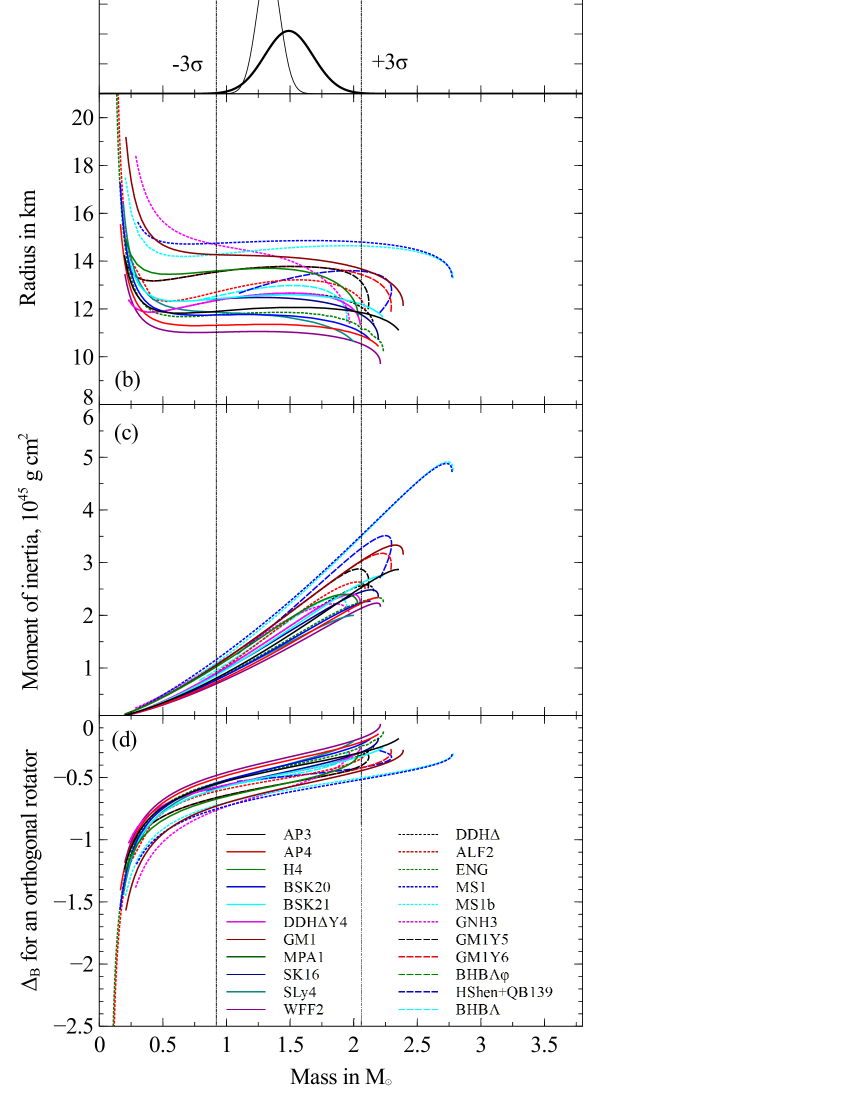
and adopt it in the calculations below. This distribution is quite wide, permitting NSs with both ‘low’ ($\sim 1.2M_{\sun}$) and ‘high’ ($\sim 1.8M_{\sun}$) masses. (It is shown in Fig. 3(a) by the thick line with its $3\sigma$ boundaries, along with the distribution of the components of DNSs derived in the same work.)

3.2 Pulsar obliquities

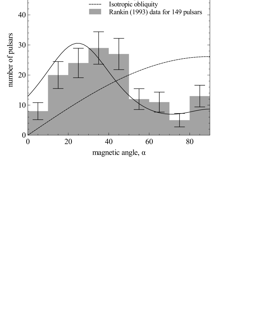
The angle $\alpha$ between the NS magnetic and spin axes has been determined for hundreds of isolated pulsars. The most confident values have been obtained for 300+ pulsars by Lyne & Manchester (1988), Rankin (1993a, b) and Gould (1994), using various methods. Tauris & Manchester (1998) combined all the measurements reported in these papers and provided an extensive analysis of their statistics. The estimations made by Rankin (1993a) were found to be fully consistent with the results published by other authors. Their distribution is shown in Fig. 1. As can clearly be seen, the apparent $p(\alpha)$ is unlikely to be isotropic, but there is evidence for a secular magnetic alignment so that most of the pulsars tend to have $\alpha\lesssim 45\degr$.

By performing an accurate statistical analysis of this data set, Zhang et al. (2003) (ZJM03 hereafter) derived an analytic equation describing the apparent $p(\alpha)$:

$$p(\alpha)=\dfrac{0.6A}{\cosh(3.5(\alpha-0.43))}+\dfrac{0.15A}{\cosh(4(\alpha-1.6))}$$ (22)

where $\alpha=0-\pi/2$ rad, and $A\approx 1.96$ is the normalization constant. We have adopted this model for the calculations below. At the same time, we also checked out the more conservative assumption about the isotropy of pulsar obliquities such that

$$p(\alpha)=\sin\alpha.$$ (23)

The important point, however, is that Spitkovsky’s spin-down model predicts the evolutionary decrease of $\alpha$ on time-scales of a few $\times$ $10^{7}$ years. Moreover, this process has been indirectly confirmed in observations with a number of statistical methods (e.g Xu & Wu, 1991; Tauris & Manchester, 1998; Weltevrede & Johnston, 2008; Young et al., 2010). Therefore one can naturally expect a non-zero correlation between the obliquity correction $\Delta_{\rm oblq}$ and the ‘magnetodipolar’ estimator $B_{\rm md}\propto\sqrt{P\dot{P}}$ over the subset of observed radiopulsars.

However, Tauris & Manchester (1998) found that the values of $P$ and $\alpha$ for 300+ pulsars do not show any significant correlation, which is probably the result of a large scatter of $\alpha$ for a given period $P$. In our work, we have also investigated the direct correlation between $\Delta_{\rm oblq}$ and $\log B_{\rm md}$ for 149 pulsars with known obliquities (Rankin, 1993a) by plotting this correlation in Fig. 2(a). The independence of these parameters is clearly seen there. It can be simply understood by assuming a weak correlation between the magnetic obliquity $\alpha_{0}$ and period $P_{0}$ at the pulsar birth and taking into account the weak dependence of the instantaneous $\dot{P}$ on $\alpha$, as predicted by the spin-down law (6).

Figure 1: The distribution of magnetic angles for 149 normal pulsars published byRankin (1993a) (grey bars) and the statistical approximation (22) found by ZJM03 (solid line). The error bars of the empirical distribution are from Poissonian statistics. The isotropic obliquity distribution (23) is also shown (dashed line).

In addition, we have undertaken numerical simulations of $\Delta_{\rm oblq}$ and $\log B_{\rm md}$ by solving the equations of pulsar spin-down using the full braking torque proposed by Philippov et al. (2014). In particular, the obliquity evolution equation

$$I\Omega\dfrac{d\alpha}{dt}=-\dfrac{\mu^{2}\Omega^{3}}{c^{3}}\sin\alpha\cos\alpha$$ (24)

has been solved simultaneously with (6) for $10^{3}$ synthetic pulsars. Initial periods $P_{0}$ were from a normal distribution centred on 300 ms with standard deviation 150 ms (Faucher-Giguère & Kaspi, 2006), magnetic moments $\log\mu$ [G cm³] $\sim{\rm normal}(30.5,1.0)$, while ages $t$were from a uniform distribution over the interval [0; 100Myr]. At the same time, while NS radii were set to 12 km for all simulated pulsars, their masses $M$ were calculated as random values according to the distribution (21) with the most probable values for the moment of inertia $I=10^{45}\cdot(M/M_{\sun})$ g cm² (see Fig. 3c).

Figure 2: The dependence of the obliquity correction$\Delta_{\rm oblq}$ on $\log B_{\rm md}$. (a) The apparent correlation for 149 pulsars with obliquities measured by (Rankin, 1993a). (b) The simulated values $\Delta_{\rm oblq}$ (11) and $\log B_{\rm md}$ in the case of isotropic obliquities $\alpha_{0}$ at pulsar birth (see text for details of the simulations). (c) The same, but for a perfect positive correlation between $\alpha_{0}$ and the initial periods $P_{0}$. (d) The same, but for a perfect negative correlation between $\alpha_{0}$ and $P_{0}$.

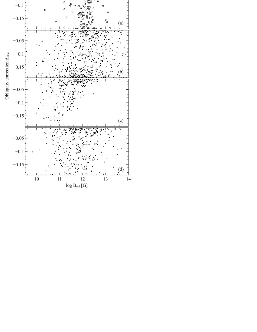
The results of the simulations are shown in Fig. 2(b)-(d). These three plots correspond to the different initial conditions adopted for the modelling: (2b) initial obliquities $\alpha_{0}$ are distributed isotropically and independently from initial periods $P_{0}$; (2c) $\alpha_{0}$ are perfectly correlated with $P_{0}$ so $\sin\alpha_{0}={\rm cdf}(P_{0}/{\rm sec})$; (2d) $\alpha_{0}$ are perfectly anti-correlated with $P_{0}$ so $\sin\alpha_{0}=1-{\rm cdf}(P_{0}/{\rm sec})$. Here ${\rm cdf}(x)$ is the cumulative distribution function of an initial period:

$${\rm cdf}(x)=\dfrac{1}{2}\left[1+{\rm erf}\left(\dfrac{x-0.3}{0.15\sqrt{2}}\right)\right]$$ (25)

and ${\rm erf}(\cdot)$ is the error function.

It has been obtained once again that $\Delta_{\rm oblq}$ do not correlate with $\log B_{\rm md}$ in all cases, except for the model in which a strong positive dependence $\alpha_{0}(P_{0})$ was adopted (Fig. 2c). Even in this case, however, the apparent correlation is very weak. Therefore, $\Delta_{\rm oblq}$ and $\log B_{\rm md}$ can be considered to be statistically independent for actual pulsars. By combining this result with the statement about the independence of $\Delta_{\rm eos}$ and $\log B_{\rm md}$ one finds the accurately calculated correction $\Delta_{\rm B}$ to be uncorrelated with the classical estimator $\log B_{\rm md}$. Hence, the width of the distribution of $\Delta_{\rm B}$ can be considered to be the same as that of the corrected value $\log B_{\rm md}+\Delta_{\rm B}$, making $\sigma[\Delta_{\rm B}]$ (15) the statistical uncertainty of the refined estimation of the magnetic field.

3.3 Realistic equations of state

The final step is the compilation of a representative subset of realistic equations of state. The recent mass measurements for pulsars PSR J1614-2230 ($1.97\pm 0.04M_{\sun}$, Demorest et al. (2010)) and J0348+0432 ($2.01\pm 0.04M_{\sun}$ Antoniadis et al. (2013)) ruled out many of the EOSs proposed earlier. In particular, for various EOSs including hyperons, the maximal mass limit for non-magnetic NSs is considerably lower than two solar masses.

There are some indications that two binaries – B1957+20 (van Kerkwijk et al., 2011) and 4U 1700-37 (Clark et al., 2002) – contain even more massive NSs with masses $\sim 2.4M_{\sun}$, even though the systematic errors of mass measurements are large. Taking into account the aforementioned examples, we excluded from our consideration EOSs for which the maximal mass of a NS is below $1.95M_{\sun}$ as being unrealistic.

Figure 3: The subset of 22 realistic equations of state of dense matter selected for the analysis. (a) The distribution of the initial masses of neutron stars (equation 21) with its $\pm 3\sigma$ boundaries is shown by the thick line, while the thin line represents the corresponding distribution for the components of double neutron stars as derived by OF16. (b) The classical mass–radius diagram. (c) Neutron star moment of inertia versus the full mass relation. (d) The correction $\Delta_{\rm B}$ (equation 9) calculated for an orthogonal rotator, that is, for constant $\Delta_{\rm oblq}\approx-0.19$. Its value is always negative for all the EOSs and lies within the interval -0.75 to -0.25 for most probable values of masses according to (21)

Unfortunately, there are no high-accuracy measurements of NS radii, and, moreover, there are no such measurements at all for any NS with a precise mass determination. Fortunately, some knowledge of the mass–radius relationship can be derived from observations and the modelling of X-ray bursts. In particular, from observations of XTE J1807-294, SAX J1808-3658, and XTE J1814-334 it can be concluded that in the wide interval of masses $1M_{\sun}<M<2.3M_{\sun}$ the radius for NSs should be approximately constant, $\sim 12$ km (Leahy et al., 2011). Other investigations (Suleimanov et al., 2011; Hambaryan et al., 2011) of longer X-ray bursts, however, witness in favour of larger radii $R\geq 14$ km. We assumed the values $11.0<R_{1.4}<15$ km for the radius of a $1.4M_{\sun}$ NS and therefore excluded from our calculations EOSs with more compact or larger stars.

For completeness of our analysis, it is necessary to consider various classes of EOSs as distinguished by the approaches used for their construction. Most EOSs fall into one of three groups, as follows.

(1) EOSs obtained from non-relativistic many-body calculations. The well-known SLy4 EOS ((Chabanat et al., 1998; Douchin & Haensel, 2001) uses a simple model of two-nucleon potential and is based on a single effective nuclear Hamiltonian. We also considered the WFF2 EOS based on the Urbana V14 two-nucleon potential (Wiringa et al., 1988) with a maximal mass of star exceeding 2$M_{\odot}$.

Models with three-nucleon interactions are based on data for energies of light nuclei and/or properties of symmetric nuclear matter (SNM) with a comparable number of neutrons and protons. We considered AP3 and AP4 EOSs (Akmal et al., 1998). These equations were obtained using variational techniques and the Argonne 18 potential plus a three-body UIX potential (AP3) and A18+UIX potentials with $\delta v$ relativistic boost corrections (AP4).

The next two unified EOSs for cold catalysed nuclear matter developed by the Brussels-Montreal group (BSK20 and BSK21, see Goriely et al. (2010); Pearson et al. (2011) and Pearson et al. (2012)) are calculated using the TETFSI method (temperature-dependent extended Thomas-Fermi plus Strutinsky integral) for functionals based on Skyrme-type forces. Recently, Gulminelli & Raduta (2015) proposed a unified EOS (SK16) using the effective interaction model and cluster energy functionals from Dobaczewski et al. (1996); Danielewicz & Lee (2009).

(2) EOSs calculated from the relativistic Dirac-Brueckner- Hartree-Fock (DBHF) approach to dense neutron matter. We considered two EOSs of this type, namely ENG (Engvik et al., 1994) and MPA1 (Müther et al., 1987) with the inclusion of contributions from the exchange of $\pi$ and $\rho$ mesons.

Figure 4: (Left) The basic moments – expectation $\langle\Delta^{\rm(eos)}_{\rm B}\rangle$ and standard deviation $\sigma[\Delta^{\rm(eos)}_{\rm B}]$ – of the distributions of correction $\Delta^{\rm(eos)}_{\rm B}$ for the subset of 22 equations of state (EOSs). The values represented by solid circles were calculated adopting the distributions of magnetic obliquity and neutron star masses described by (22) and (21) respectively. Open circles, in turn, assume the model (23) of isotropically distributed obliquities. Some points are labelled with the name of the corresponding EOS. It is clear that, while the average of $\Delta_{\rm B}$ covers the interval from $\approx-$0.55 to $\approx-$0.25, its dispersion remains approximately the same for all EOSs with the typical value $\sigma[\Delta^{\rm(eos)}_{\rm B}]\sim 0.07$. This value represents the reachable precision of a timing-based estimation of a pulsar magnetic field within unknown obliquity and the mass of a neutron star. (Right) The distributions of $p(\Delta_{\rm B}|{\rm eos})$ for 22 equations of state within the ZJM03 obliquities (grey lines). The distributions of the generalized correction $p(\Delta^{*}_{\rm B})$ adopting the ZJM03 model and isotropic obliquities are shown by the solid and dashed black curves respectively. All the plotted distributions are roughly close to the normal one.

(3) EOSs from relativistic mean-field theoretical models (RMFs). In particular, we take for calculations the well-known GM1 EOS (Glendenning & Moszkowski, 1991)). This EOS is based on the classical parametrization proposed by Glendenning and Moszkowski. More realistic models predict the existence of hyperons in NS cores at densities of $5-8\times 10^{14}$ g/cm³. Two extensions of the GM1 model, GM1Y5 and GM1Y6 (Oertel et al., 2015), are obtained for cold NS matter in $\beta$-equilibrium containing the baryon octet and electrons.

Another RMF parametrization, DDH$\delta$, was considered by Gaitanos et al. (2004). Its extension on the hyperon (DDH$\Delta$4 EOS) sector in the same manner as for the GM1 model is proposed in Grill et al. (2014). BHB$\Lambda$ EOS and its variation BHB$\Delta\phi$ EOS (Banik et al., 2014) are obtained from the statistical model of Hempel & Schaffner-Bielich (2010) with RMF parametrization DD2 (Typel et al., 2010), extended by $\Lambda$-hyperons or $\Lambda$-hyperons interacting via the $\phi$-meson. We also consider EOSs proposed by Mueller and Serot (Müller & Serot, 1996) (MS1, MS1b) taking account of the non-linear interactions between the scalar-isoscalar ($\sigma$), vector-isoscalar ($\omega$), and vector-isovector ($\rho$) fields

The family of GNH EOSs with nucleon-hyperon composition was proposed by (Glendenning, 1985). We use the GNH3 EOS with universal couplings for hyperons in our calculations. This EOS gives an acceptable upper limit of mass for a star.

Seven hyperonic EOSs in relativistic mean field theory were proposed by Nayyar & Owen (2006). Only one of these equations – namely H4 – is consistent with the two-solar-mass limit. In contrast to the GNH3 EOS, the hyperon-meson couplings for H4 are assumed to be the same for all hyperons but are weaker than the nucleon-meson couplings. The stiffness is achieved owing to the high value of incompressibility, K = 300 MeV

It cannot be ruled out that some compact stars are ‘hybrid stars’ with cores consisting of quark matter. However, many such EOSs are not compatible with the upper mass limit and radius constraints. Two hybrid EOSs with nuclear matter and colour-flavour-locked quark matter are included in our consideration. The ALF2 EOS was proposed by Alford et al. (2005). As shown for acceptable parameters of the MIT bag model with gluonic corrections, one can obtain a mass–radius relationship for hybrid stars similar to that predicted for stars from nucleonic matter. For nuclear matter, the EOS proposed by Akmal, Pandharipande and Ravenhall (APR) was used

The HShen+QB139 EOS (Sagert et al., 2009; Sagert et al., 2010; Fischer et al., 2011) is based on the model proposed by Shen et al. (1998) with the addition of a bag model for the quark phase. The transition to quark matter has been described in the frame of the non-linear RMF model with TM1 parametrization (Sugahara & Toki, 1994).

Thus, we have finally compiled a list of 22 EOSs that we consider to be representative enough for the current state of knowledge. The basic parameters of NSs as well as the mass–radius and mass– moment of inertia relationships were calculated for each equation. The basics of EOS calculus can be found in Appendix  A, while the results are shown in Table 2 and in Fig. 3(b) and (c). The correction $\Delta_{\rm B}$ in the case of an orthogonal rotator ($\alpha=90\deg$) was also calculated and is shown in Fig. 3(d).

It can be seen that EOSs from the DBHF approach give results similar to non-relativistic EOSs from many-body calculations (these EOSs are listed in Table 2 above the horizontal line). The radii for a NS with canonical mass $1.4M_{\odot}$ vary from 11.04 km (WFF2) to 12.58 km (BSK21), and the moment of inertia of such a star lies in a narrow interval $1.28<I(1.4M_{\odot})<1.57\times 10^{45}$ g cm². For RMF EOSs we have relatively larger radii, $R\sim 13-14$ km, and the interval for the moment of inertia $1.74<I(1.4M_{\odot})<2.05\times 10^{45}$ g cm². We also include in the table the results for stars with $M=1.49M_{\odot}$. Therefore, the canonical value for $I(1.4M_{\odot})=10^{45}$ g cm² seems to underestimate the actual values of NSs moments of inertia for 30-60 per cent at least.

4 Properties of the refined estimator

We have calculated numerically the distributions of $\Delta^{\rm(eos)}_{\rm B}$ and their basic moments for all the EOSs described above. The values of $M$ and $\alpha$ have been simulated $10^{5}$ times for each run according to the empirical distributions of these quantities discussed in Sections  3.1 and 3.2 respectively.

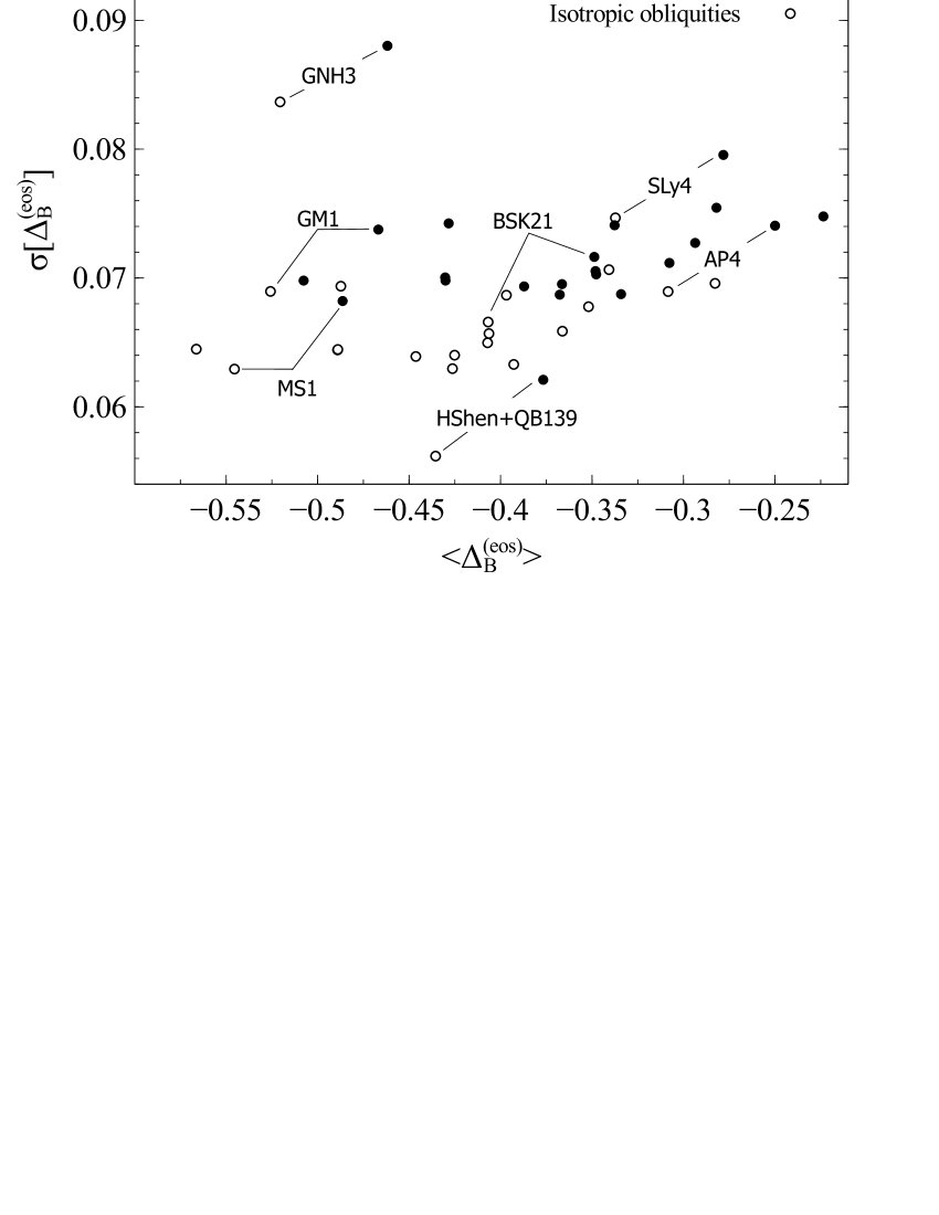
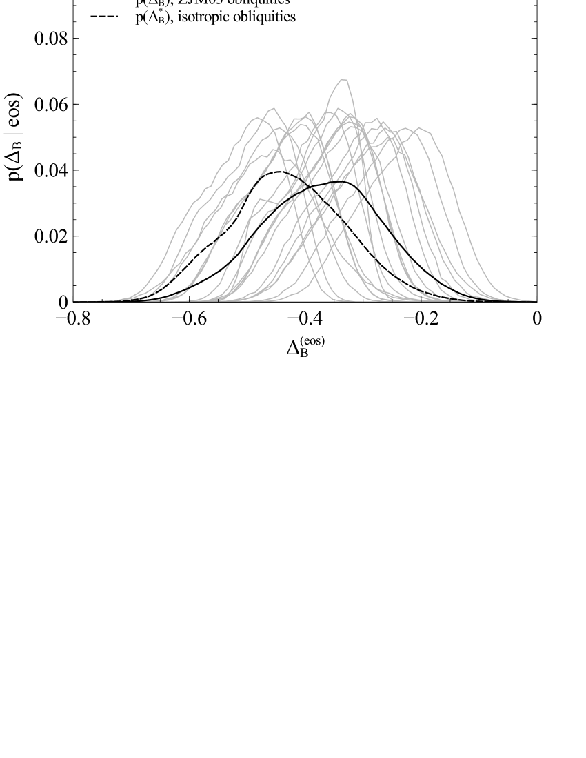
The results are shown in Fig. 4. Adopting the ZJM03 model of pulsar obliquities, the shape of $p(\Delta_{\rm B}|{\rm eos})$ was found to be very close to the Gaussian for every EOS (see the right panel of the figure). The corresponding means$\langle\Delta^{\rm(eos)}_{\rm B}\rangle$ cover a relatively narrow interval of values from $\approx-0.51$ (for MS1) to $\approx-0.23$ (for WFF2), while the standard deviations $\sigma[\Delta^{\rm(eos)}_{\rm B}]$ appear to be nearly the same for all equations:

$$\sigma[\Delta^{\rm(eos)}_{\rm B}]\approx 0.07\pm 0.01.$$ (26)

The latter result seems to be the consequence of two factors. The first is the existence of a flat plateau in $R(M)$ relationships, which is typical for the considered EOSs. In other words, all isolated NSs are likely to have the same radii within the adopted distribution of their masses. The second factor is that the pulsar spin-down luminosity weakly depends on the instant obliquity $\alpha$, which makes the distribution of $\Delta_{\rm oblq}(\alpha)$ quite narrow. Indeed, when adopting the spin-down law that is strongly dependent on $\alpha$ ($x_{\perp}=2/3$, $x_{\parallel}=0$ so $P\dot{P}\propto B^{2}\sin^{2}\alpha$ in the terms of equations (2) and (3)), we obtained typical $\sigma[\Delta^{\rm(eos)}_{\rm B}]\approx 0.36$, which is five times greater than (26).

On the other hand, if the isotropic distribution of $\alpha$ is used, the distributions $p(\Delta_{\rm B}|{\rm eos})$ keep their shapes and widths in general. The corresponding means $\langle\Delta^{\rm(eos)}_{\rm B}\rangle$ are just shifted by $\sim$0.05 to the left relative to the points given by the ZJM03 model (as shown by open circles in the same panel). So, we conclude that the specific choice of $p(\alpha)$ does not affect significantly the results of the calculations of the correction $\Delta_{\rm B}^{\rm(eos)}$.

Finally, the distribution of the generalized correction $\Delta^{*}_{\rm B}$ under the assumption of equal weights (we used $w_{i}=1/22$) of every EOS from our list was also calculated. The resulting curves are shown with the black solid (for ZJM03) and dashed (for isotropic $p(\alpha)$) lines in the right panel of Fig. 4. For the ZJM03 model of pulsar obliquities we found that

$$\log B^{\rm*}-\log B_{\rm md}\approx-0.37\pm 0.10,$$ (27)

while isotropic model gave

$$\log B^{\rm*}-\log B_{\rm md}\approx-0.43\pm 0.10.$$ (28)

This result means that the timing-based estimation of a pulsar magnetic field can be as precise as $\sim 0.1$ dex even if neither the EOS nor the mass nor the obliquity is known. It is an intrinsic property of the adopted pulsar spin-down luminosity model. If it is rewritten in a linear form, the quantity

$$B^{*}\approx\frac{3}{7}B_{\rm md}$$ (29)

provides an unbiased estimation of the actual surface magnetic field strength of an isolated radiopulsar with only $\sim$20-25 per cent uncertainty at the 68 per cent confidence level.

5 Discussion

5.1 Do pulsars timing irregularities affect $\log B$?

We have hitherto assumed that the instantaneous NS magnetic field $B$ is linked to the observed $P$ and $\dot{P}$ through the spin-down law (6) in the strict sense. However, the actually observed spin evolution of isolated pulsars is more complex than predicted by that equation. The spin-down rate appears to be significantly contaminated by additional irregular, quasi-periodic variations on short time-scales from months to years that are typically referred to as the ‘timing noise’ (Boynton et al., 1972; Cordes & Helfand, 1980; D’Alessandro et al., 1995; Urama et al., 2006; Hobbs et al., 2010; Nice et al., 2013).

The strength of this unmodelled component of the pulsar spindown can be characterized numerically with the dimensionless combination

$$n=\dfrac{\ddot{\Omega}\Omega}{\dot{\Omega}^{2}}$$ (30)

– the so-called “braking index’. Differentiating the general spin-down law (3), gives

$$n=3+\dfrac{\Omega}{\dot{\Omega}}\left[2\dfrac{1}{\mu}\dfrac{{\rm d}\mu}{{\rm d}t}-\dfrac{1}{I}\dfrac{{\rm d}I}{{\rm d}t}+\dfrac{1}{f}\dfrac{{\rm d}f}{{\rm d}\alpha}\dot{\alpha}\right],$$ (31)

where the first term reflects the power of the $\Omega$ term in the braking torque equation (1). In other words, if the spin-down of a NS follows the expression $\dot{\Omega}=-K\Omega^{q}$, then the combination (30) is simply equal to $q$ assuming constant $K$.

Thus, $n\in 3..3.25$ for the Spitkovsky’s law when magnetic moment $\mu$ and moment of inertia $I$ are fixed but the obliquity $\alpha$ decreases according to (24) (e.g. Ekşi et al., 2016). Other models for $f(\alpha)$ and $\dot{\alpha}$ are able to significantly extend this interval up to $0\la n\la 10^{4}$. For instance, the classical magneto-dipolar losses ($x_{\perp}=2/3$, $x_{\parallel}=0$) give $n=3+2\cot^{2}\alpha\la 10^{3}$ for actual pulsars.

Nevertheless, the estimated values of $n$ for hundreds of pulsars are surprisingly far from any prediction. Their values have been found in the range from $\sim-10^{6}$ to $\sim 10^{6}$, being negative for about half of the objects (e.g Hobbs et al., 2004; Biryukov et al., 2012; Zhang & Xie, 2012). So, they are unlikely to represent the secular (i.e. evolutionary) spin-down of radiopulsars.

Note that the braking indices of most of the sources are not stable from observation to observation. Even for a few tens of ‘lownoise’ pulsars, however, the values of $n$ are constant within spans of 10-30 years but still extremely anomalous (Biryukov et al., 2007). Thus, finally, only 10 sources are accepted to date as having meaningful and stable $n\in 0.03$-$3.15$ that can be interpreted in terms of the spin-down law (3) (Archibald et al., 2016; Marshall et al., 2016).

Although the physics of the pulsar timing irregularities remains generally unclear, the proposed solutions of the ‘anomalous braking indices’ problem can be qualitatively divided into two categories. Type I models incorporate the relatively slow variability of NS parameters directly in the spin-down equation, assuming the variability of the surface magnetic field (Pons et al., 2012; Zhang & Xie, 2012; Ou et al., 2016), obliquity (Melatos, 2000; Lyne et al., 2013; Arzamasskiy et al., 2015) or effective moment of inertia (Tsang & Gourgouliatos, 2013; Hamil et al., 2015; Hamil et al., 2016). Such models strictly keep the relationship between the observed $P$, $\dot{P}$ and $B$ in the form of the adopted spin-down law at any moment of time. Hence, the timing-based magnetic field estimation $B\propto\sqrt{P\dot{P}}$ cannot be affected by the processes of such a type.

Type II models suggest the existence of an additional either quasi-periodic or purely stochastic component $\delta\dot{\Omega}$in the spindown rate. The underlying physics was proposed to be probably connected with the magnetospheric perturbations (Cheng, 1987; Kramer et al., 2006; Contopoulos, 2007; Lyne et al., 2010), or processes in the star interior (Janssen & Stappers, 2006; Melatos & Link, 2014), or to be the imprint of the so-called ‘anomalous braking torque’ (Biryukov et al., 2007; Barsukov & Tsygan, 2010; Biryukov et al., 2012). Within this approach, the observed spin frequency derivative $\dot{\Omega}_{\rm obs}$ is the sum of $\dot{\Omega}\propto B^{2}\Omega^{3}(1+1.4\sin^{2}\alpha)$ and the variational term

$$\dot{\Omega}_{\rm obs}=\dot{\Omega}+\delta\dot{\Omega}=\dot{\Omega}\left(1+\varepsilon\right),$$ (32)

where $\varepsilon(t)=\delta\dot{\Omega}/\dot{\Omega}$ is the relative divergence. Note, that the corresponding divergence of the spin frequency $\delta\Omega=\Omega_{\rm obs}-\Omega$ is assumed to be vanishingly small and can be neglected.

Generally, the wide range of the models proposed for $\delta\dot{\Omega}$ cannot explain the properties of the observed braking indices completely (Malov, 2016). Formally, Type II solutions require the correction $\Delta^{\rm(eos)}_{\rm B}$ (9) to be extended by the additional term

$$\Delta_{\varepsilon}=-\dfrac{\log(1-\varepsilon)}{2}$$ (33)

because $\delta\dot{P}/\dot{P}=-\delta\dot{\Omega}/\dot{\Omega}=-\varepsilon$. Moreover, because it is not possible to reject the hypothesis that both types of physical processes (I and II) can contribute to the unmodelled part of the observed spin-down, the term $\Delta_{\varepsilon}$ has to be added to $\Delta^{\rm(eos)}_{\rm B}$ as

$$\Delta^{\rm(eos)}_{\rm B,ext}=\Delta^{\rm(eos)}_{\rm B}+r_{\rm ext}\Delta_{\varepsilon},$$ (34)

where $r_{\rm ext}\in 0...1$ characterizes the ‘fraction’ of the unmodeled spin-down from the Type II (i.e. external) processes. For instance, $r_{\rm ext}=0$ means that anomalous braking indices can be explained by the $\mu$, $I$ and/or $\alpha$ variations only using equation (31).

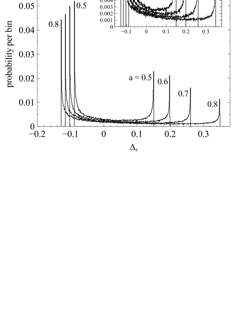
The extensive analysis of pulsar complex rotation undertaken by Hobbs et al. (2010) showed that $\delta\dot{\Omega}$ is unlikely to be dominated by a stochastic process. Instead, the observed timing noise patterns show nearly periodic features. If this is the case, then the amplitude of relative variations $\varepsilon$ can be estimated empirically from the statistics of the observed second derivatives of pulsar spin frequencies $\ddot{\Omega}_{\rm obs}=\ddot{\Omega}+\delta\ddot{\Omega}$ , assuming them to be almost completely dominated by the $\delta\ddot{\Omega}$ term. The corresponding analysis has been undertaken by Biryukov et al. (2012) and has shown that

$$0.5\la\max|\varepsilon|\la 0.8$$ (35)

is able to reproduce the observed correlations between the pulsar timing parameters. Such amplitudes may lead to very high, up to $\sim 0.35$, values of the $\Delta_{\varepsilon}$ correction, and are also slightly asymmetric with respect to $\Delta_{\varepsilon}=0$. We plot the possible distributions of this quantity in Fig.  5, assuming $\varepsilon=a\cos\varphi$ for various $a$ and random $\varphi$, as has been done by Biryukov et al. (2012). Thus, the term $\Delta_{\varepsilon}$ can, in principle, be a major source of the uncertainty in the timing-based magnetic field estimation.

Figure 5: The simulated distributions of the correction $\Delta_{\varepsilon}$ (33) assuming a simple cyclic process for $\delta\dot{\Omega}/\dot{\Omega}=\varepsilon=a\cos\varphi$. The distributions are calculated for $a=0.5,0.6,0.7$ and $0.8$, while the cyclic phase $\varphi$ is assumed to be random over the interval $0-2\pi$. The sharp peaks at the boundary values are caused by the harmonic nature of $\varepsilon$ (the cyclic variable spends more time at its extrema) and the logarithmic nature of the relationship $\Delta_{\varepsilon}(\varepsilon)$. See Section 5.1 for details.

On the other hand, there are some indirect arguments in favour of the idea that the pulsar secular spin-down follows the law (3) with small typical values of $\varepsilon$. Thus, it has been shown many times that the observable parameters of Galactic pulsars can be well reproduced within a population synthesis adopting (3) with various forms of $f(\alpha)$ (e.g Faucher-Giguère & Kaspi, 2006; Ridley & Lorimer, 2010; Gullón et al., 2014) and neglecting the corrections due to $\varepsilon\neq 0$. Moreover, the model-independent analysis of pulsar kinetics on the $P-\dot{P}$ diagram resulted in a reasonable value of their birthrate of $\la 1$ century^-1, simply assuming $f(\alpha)\equiv 1$ (Keane & Kramer, 2008; Vranešević & Melrose, 2011) and $\varepsilon\equiv 0$.

Finally, it basically remains unclear whether the correction $\Delta_{\varepsilon}$ should really be taken into account, because the value of the fraction $r_{\rm ext}$ remains completely unknown.

5.2 Astrophysical implications

Accurate and precise measurements of NS surface magnetic fields are important in many areas, in particular for the investigation of the field evolution $B(t)$ for normal, rotation-powered pulsars. The NS magnetic field decay has been predicted in many theoretical works (Ostriker & Gunn, 1969; Goldreich & Reisenegger, 1992; Cumming et al., 2004; Pons et al., 2007; Geppert, 2009; Viganò et al., 2013; Igoshev & Popov, 2015). On the other hand, simulations of the observed pulsar population by Faucher-Giguère & Kaspi (2006) have shown that the statistics of basic observed pulsar parameters can be well reproduced without the assumption of the evolution of the magnetic field. This contradiction can in principle be solved by the direct probing of the magnetic field evolution of normal pulsars.

Indeed, it is expected that the surface $B$ strength decreases down to one order of magnitude during the pulsar lifetime. This is much greater than the typical uncertainty of the refined estimator $\log B_{\rm md}+\Delta^{\rm(eos)}_{\rm B}$, and three times greater if the maximal $\Delta_{\varepsilon}$ is adopted. At the same time, the average correction $\langle\Delta^{\rm(eos)}_{\rm B}\rangle$ remains common for all pulsars within a given EOS. So, the shape of an apparent field evolution $\log B^{\rm(eos)}(t)$ does not depend on the choice of the specific EOS. This, however, is not true for the average value of the initial field $\log B^{\rm(eos)}(0)$.

We will present the results of our research into the empirical magnetic field evolution for normal radiopulsars with independently measured ages in a forthcoming paper.

The precise magnetic field measurements can also be useful when the specific threshold value of $B$ exists within a problem. Thus, there are 16 high-B isolated normal pulsars in the ATNF data base with the standard magnetic field $B_{\rm md}$ at the pole greater than the Schwinger quantum limit of $\approx 4.4\times 10^{13}$ G. However, according to the refined $B$ estimator we propose that there is only one (for BSK21) or even zero (for MS1) such extreme objects at the 99.7 per cent confidence level assuming $r_{\rm ext}=0$.

Finally, the so-called pulsar ‘deathline’ depends on both the current value of the magnetic field and on the spin period of a radiopulsar (e.g Ruderman & Sutherland, 1975; Chen & Ruderman, 1993; Kantor & Tsygan, 2004). Thus, the population of ‘zombie’-pulsars can be investigated within a given EOS, if the corrected value of $B$ is adopted.

6 Conclusions

The basic results of our research are as follows:

1. The refined version of the canonical timing-based estimator of the surface magnetic field of normal radiopulsars $B_{\rm md}(P,\dot{P})$ was introduced in a form $\log B=\log B_{\rm md}+\Delta^{\rm(eos)}_{\rm B}$. The correction $\Delta^{\rm(eos)}_{\rm B}$ is generally dependent on the given EOS, the NS mass $M$ and the obliquity $\alpha$.

2. It was found that within existing observational constraints on masses $M$ and obliquities $\alpha$ of isolated radiopulsars, the value of this correction is distributed almost normally with the standard deviation as small as $\approx 0.06..0.09$ dex for most of realistic EOSs. The average value of $\Delta^{\rm(eos)}_{\rm B}$ is, however, non-zero and covers the range from $\approx-0.55$ to $\approx-0.25$, depending on the choice of EOS.

3. The generalized timing-based estimator $\log B^{*}=\log B_{\rm md}-0.37\pm 0.10$ was also introduced under the assumption of equal chances for all 22 considered EOSs to be realized in nature. It indicates that within the Spitkovsky’s spin-down Law (6) the magnetic field of an arbitrary radiopulsar can be measured with $\lesssim 30\%$ relative error using the timing parameters only.

4. The pulsar timing noise can, in principle, affect the timing-based measurement of pulsar magnetic field, so additional correction term $r_{\rm ext}\Delta_{\varepsilon}$ has to be taken into account. While the value of $\Delta_{\varepsilon}$ can be as large as $\sim 0.35$, the fraction of the timing noise due to external physical processes (relative to the secular spin-down law (6)) $r_{\rm ext}\in 0..1$ remains completely unknown.

Appendix A Calculations of the parameters of a neutron star

Let us consider the basic moments of calculations of NS parameters. Note that a simple estimation of the Kepler frequency $\Omega_{k}\approx\sqrt{GM/R^{3}}$ shows that for $M=1.4M_{\odot}$ its value lies between 7.4 and 16 kHz for $9<R<15$ km. The frequencies of rotation for the considered pulsars are much lower, and therefore the slow-rotation approximation can be used for solving the general relativity equations. The stellar configurations are assumed to be spherical. The space-time metric with only first-order rotational terms with respect to the stellar angular velocity ${\Omega}$ can be written as

Table 2: The parameters of neutron stars for various equations of state discussed in the paper. Neutron stars radii and moments of inertia for the $M=1.4M_{\odot}$ and $M=1.49M_{\odot}$ are shown, as well as the maximal mass limit for corresponding equation of state. The means $\langle\cdot\rangle$ and standard deviations $\sigma[\cdot]$ of the correction $\Delta_{\rm B}^{\rm(eos)}$ are calculated adopting the mass distribution (21) and anisotropic obliquities (22). The horizontal line separate equations of state based on the DBHF approach and many-body calculations (above) from ones based on relativistic mean field theory (below).

		$M=1.4M_{\sun}$		$M=1.49M_{\sun}$
EOS	$M_{\rm max}/M_{\sun}$	$R$, km	$I_{45}$	$R$, km	$I_{45}$	$\langle\Delta_{\rm B}^{\rm(eos)}\rangle$	$\sigma[\Delta_{\rm B}^{\rm(eos)}]$
SLy4	2.05	11.69	1.36	11.62	1.49	-0.279	0.080
WFF2	2.21	11.04	1.28	11.03	1.39	-0.224	0.075
BSK20	2.17	11.74	1.38	11.71	1.53	-0.283	0.075
BSK21	2.28	12.58	1.57	12.58	1.73	-0.349	0.072
AP3	2.38	12.06	1.49	12.06	1.63	-0.308	0.071
AP4	2.19	11.36	1.33	11.29	1.44	-0.250	0.074
SK16	2.19	12.47	1.53	12.44	1.69	-0.338	0.074
MPA1	2.49	12.39	1.57	12.41	1.70	-0.334	0.069
ENG	2.23	11.85	1.42	11.86	1.54	-0.293	0.072
GM1	2.39	14.19	1.85	14.17	2.03	-0.467	0.074
GM1Y5	2.12	13.78	1.86	13.78	2.03	-0.430	0.070
GM1Y6	2.30	13.78	1.86	13.78	2.03	-0.430	0.069
DDH$\Delta$	2.16	12.65	1.63	12.65	1.78	-0.348	0.070
DDH$\Delta Y$4	2.05	12.65	1.63	12.65	1.78	-0.348	0.071
BHB$\Lambda\phi$	2.10	12.95	1.74	12.98	1.90	-0.367	0.069
BHB$\Lambda$	1.95	12.96	1.74	12.98	1.90	-0.366	0.069
MS1	2.77	14.83	2.05	14.85	2.25	-0.507	0.070
MS1b	2.78	14.52	2.00	14.55	2.20	-0.487	0.068
GNH3	1.97	14.18	1.80	14.00	1.94	-0.462	0.087
H4	2.03	12.87	1.84	12.99	1.98	-0.428	0.074
ALF2	2.09	13.17	1.74	13.20	1.91	-0.388	0.069
HShen+QB139	2.30	13.16	1.91	13.27	2.07	-0.377	0.062

$$ds^{2}= -e^{2\psi(r)}c^{2}dt^{2}+e^{2\lambda(r)}dr^{2}+$$ (36)

$$r^{2}\left(d\theta^{2}+\sin^{2}\theta\left(d\phi^{2}-2(\Omega-\omega(r,\theta))d\phi dt\right)\right).$$

Here $\psi$ and $\lambda$ are the functions of radial coordinate only. The value $\hat{\omega}=\Omega-\omega(r,\theta)$ is nothing else than the angular velocity of zero-angular-momentum observer. The Einstein equations are

$$R_{\mu\nu}-\frac{1}{2}g_{\mu\nu}R=\frac{8\pi G}{c^{4}}T_{\mu\nu}.$$ (37)

Here $R_{\mu\nu}$ is Ricci tensor for the metric $g_{\mu\nu}$, $R$ is the scalar curvature and $T_{\mu\nu}$ is the energy-momentum tensor for stellar matter. For the case of spherical symmetry

$$T^{\mu}_{\nu}=(\rho c^{2}+p)u^{\mu}u_{\nu}-p\delta^{\mu}_{\nu},$$ (38)

where $u^{\mu}$ is the matter 4-velocity. For axial symmetry and uniform rotation we have for $u^{\mu}$ the following relation:

$$u^{\mu}=u^{t}(1,0,0,\Omega).$$ (39)

Here $\rho$ and $p$ are density and pressure of matter respectively. Keeping only first order terms with respect to $\hat{\omega}$ one can write the components of the field equations as

$$\frac{1}{r^{2}}\frac{d}{dr}\left[r\left(1-e^{-2\lambda}\right)\right]=8\pi G\rho\/c^{2},$$ (40)

$$\frac{1}{r}\left[2e^{-2\lambda}\frac{d\psi}{dr}-\frac{1}{r}\left(1-e^{-2\lambda}\right)\right]=8\pi pG/c^{4}.$$ (41)

Taking into account the hydrostatic equilibrium condition

$$\frac{dp}{dr}=-(\rho c^{2}+p)\frac{d\psi}{dr}$$ (42)

and definition of gravitational mass $m(r)$ according to the relationship

$$e^{-2\lambda(r)}=1-\frac{2Gm(r)}{c^{2}r}$$ (43)

it can be concluded that the equations above are nothing other than the ordinary Tolmen-Oppenheimer-Volkoff equations.

For $\omega(r,\theta)$ we have the equation

$$\frac{e^{\psi-\lambda}}{r^{4}}\partial_{r}\left[e^{-(\psi+\lambda)}r^{4}\partial_{r}{\omega}\right]+\frac{1}{r^{2}\sin^{3}\theta}\partial_{\theta}\left[\sin^{3}\theta\partial_{\theta}\omega\right]=$$ (44)

$$\frac{16\pi G}{c^{4}}(\rho c^{2}+p){\omega}.$$

For asymptotically flat space-time, the angular velocity is a function of the radial coordinate only and therefore equation (44) can be rewritten as

$$\frac{e^{\psi-\lambda}}{r^{4}}\frac{d}{dr}\left[e^{-(\psi+\lambda)}r^{4}\frac{d{\omega}}{dr}\right]=\frac{16\pi G}{c^{4}}(\rho c^{2}+p){\omega}.$$ (45)

At $r\rightarrow\infty$, the following condition on $\omega(r)$ should be satisfied:

$$\lim_{r\to\infty}{\omega(r)}={\Omega}.$$ (46)

Finally, the regularity condition at the center of a star requires that

$$\frac{d{\omega}(0)}{dr}=0.$$ (47)

The moment of inertia is defined via the angular momentum $J$ according to the relationship

$$I\equiv\frac{J}{\Omega}.$$ (48)

The Angular moment is

$$J=\int T^{\mu}_{\nu}\xi^{\nu}_{(\phi)}\sqrt{-g}d^{3}x.$$ (49)

Here $\xi^{\nu}_{(\phi)}$ is the Killing vector in the azimuthal direction. Keeping only terms of first order in ${\omega}$ the moment of inertia can be evaluated as

$$I\approx\frac{8\pi}{3}\int_{0}^{R}(\rho+p/c^{2})e^{\lambda-\psi}r^{4}\frac{{\omega}}{\Omega}dr.$$ (50)

Therefore the moment of inertia in the slow-rotation approximation is independent from the angular velocity.

References

- Akmal et al. (1998) Akmal A., Pandharipande V. R., Ravenhall D. G., 1998, Phys. Rev. C, 58, 1804
- Alford et al. (2005) Alford M., Braby M., Paris M., Reddy S., 2005, ApJ, 629, 969
- Antoniadis (2013) Antoniadis J. I., 2013, PhD thesis, University of Bonn
- Antoniadis et al. (2013) Antoniadis J., et al., 2013, Science, 340, 448
- Antoniadis et al. (2016) Antoniadis J., Tauris T. M., Özel F., Barr E., Champion D. J., Freire P. C. C., 2016, preprint, (arXiv:1605.01665)
- Archibald et al. (2016) Archibald R. F., et al., 2016, ApJ, 819, L16
- Arzamasskiy et al. (2015) Arzamasskiy L., Philippov A., Tchekhovskoy A., 2015, MNRAS, 453, 3540
- Arzamasskiy et al. (2017) Arzamasskiy L. I., Beskin V. S., Pirov K. K., 2017, MNRAS, 466, 2325
- Banik et al. (2014) Banik S., Hempel M., Bandyopadhyay D., 2014, ApJS, 214, 22
- Barsukov & Tsygan (2010) Barsukov D. P., Tsygan A. I., 2010, MNRAS, 409, 1077
- Barsukov et al. (2009) Barsukov D. P., Polyakova P. I., Tsygan A. I., 2009, Astronomy Reports, 53, 1146
- Beskin (2016) Beskin V. S., 2016, preprint, (arXiv:1610.03365)
- Beskin & Nokhrina (2007) Beskin V. S., Nokhrina E. E., 2007, Ap&SS, 308, 569
- Beskin et al. (1993) Beskin V. S., Gurevich A. V., Istomin Y. N., 1993, Physics of the pulsar magnetosphere. Cambridge, New York: Cambridge University Press
- Beskin et al. (2013) Beskin V. S., Istomin Y. N., Philippov A. A., 2013, Physics Uspekhi, 56, 164
- Biryukov et al. (2007) Biryukov A., Beskin G., Karpov S., Chmyreva L., 2007, Advances in Space Research, 40, 1498
- Biryukov et al. (2012) Biryukov A., Beskin G., Karpov S., 2012, MNRAS, 420, 103
- Borghese et al. (2015) Borghese A., Rea N., Coti Zelati F., Tiengo A., Turolla R., 2015, ApJ, 807, L20
- Boynton et al. (1972) Boynton P. E., Groth E. J., Hutchinson D. P., Nanos Jr. G. P., Partridge R. B., Wilkinson D. T., 1972, ApJ, 175, 217
- Chabanat et al. (1998) Chabanat E., Bonche P., Haensel P., Meyer J., Schaeffer R., 1998, Nuclear Physics A, 635, 231
- Chashkina & Popov (2012) Chashkina A., Popov S. B., 2012, New Astron., 17, 594
- Chen & Ruderman (1993) Chen K., Ruderman M., 1993, ApJ, 402, 264
- Cheng (1987) Cheng K. S., 1987, ApJ, 321, 799
- Clark et al. (2002) Clark J. S., Goodwin S. P., Crowther P. A., Kaper L., Fairbairn M., Langer N., Brocksopp C., 2002, A&A, 392, 909
- Contopoulos (2007) Contopoulos I., 2007, A&A, 475, 639
- Contopoulos & Spitkovsky (2006) Contopoulos I., Spitkovsky A., 2006, ApJ, 643, 1139
- Cordes & Helfand (1980) Cordes J. M., Helfand D. J., 1980, ApJ, 239, 640
- Cumming et al. (2004) Cumming A., Arras P., Zweibel E., 2004, ApJ, 609, 999
- D’Alessandro et al. (1995) D’Alessandro F., McCulloch P. M., Hamilton P. A., Deshpande A. A., 1995, MNRAS, 277, 1033
- Danielewicz & Lee (2009) Danielewicz P., Lee J., 2009, Nuclear Physics A, 818, 36
- Davis & Goldstein (1970) Davis L., Goldstein M., 1970, ApJ, 159
- Demorest et al. (2010) Demorest P. B., Pennucci T., Ransom S. M., Roberts M. S. E., Hessels J. W. T., 2010, Nature, 467, 1081
- Deutsch (1955) Deutsch A. J., 1955, Annales d’Astrophysique, 18, 1
- Dobaczewski et al. (1996) Dobaczewski J., Nazarewicz W., Werner T. R., Berger J. F., Chinn C. R., Dechargé J., 1996, Phys. Rev. C, 53, 2809
- Douchin & Haensel (2001) Douchin F., Haensel P., 2001, A&A, 380, 151
- Ekşi et al. (2016) Ekşi K. Y., Andaç I. C., Çıkıntoğlu S., Gügercinoğlu E., Vahdat Motlagh A., Kızıltan B., 2016, ApJ, 823, 34
- Engvik et al. (1994) Engvik L., Hjorth-Jensen M., Osnes E., Bao G., Østgaard E., 1994, Physical Review Letters, 73, 2650
- Faucher-Giguère & Kaspi (2006) Faucher-Giguère C.-A., Kaspi V. M., 2006, ApJ, 643, 332
- Finn (1994) Finn L. S., 1994, Physical Review Letters, 73, 1878
- Fischer et al. (2011) Fischer T., et al., 2011, ApJS, 194, 39
- Gaitanos et al. (2004) Gaitanos T., Di Toro M., Typel S., Baran V., Fuchs C., Greco V., Wolter H. H., 2004, Nuclear Physics A, 732, 24
- Geppert (2009) Geppert U., 2009, in Becker W., ed., Vol. 357, Astrophysics and Space Science Library. p. 319 (arXiv:astro-ph/0611708)
- Glendenning (1985) Glendenning N. K., 1985, ApJ, 293, 470
- Glendenning & Moszkowski (1991) Glendenning N. K., Moszkowski S. A., 1991, Physical Review Letters, 67, 2414
- Goldreich & Julian (1969) Goldreich P., Julian W. H., 1969, ApJ, 157, 869
- Goldreich & Reisenegger (1992) Goldreich P., Reisenegger A., 1992, ApJ, 395, 250
- Good & Ng (1985) Good M. L., Ng K. K., 1985, ApJ, 299, 706
- Goriely et al. (2010) Goriely S., Chamel N., Pearson J. M., 2010, Phys. Rev. C, 82, 035804
- Gould (1994) Gould D. M., 1994, PhD thesis, Univ. of Manchester
- Grill et al. (2014) Grill F., Pais H., Providência C., Vidaña I., Avancini S. S., 2014, Phys. Rev. C, 90, 045803
- Gullón et al. (2014) Gullón M., Miralles J. A., Viganò D., Pons J. A., 2014, MNRAS, 443, 1891
- Gulminelli & Raduta (2015) Gulminelli F., Raduta A. R., 2015, Phys. Rev. C, 92, 055803
- Hambaryan et al. (2011) Hambaryan V., Suleimanov V., Schwope A. D., Neuhäuser R., Werner K., Potekhin A. Y., 2011, A&A, 534, A74
- Hamil et al. (2015) Hamil O., Stone J. R., Urbanec M., Urbancová G., 2015, Phys. Rev. D, 91, 063007
- Hamil et al. (2016) Hamil O., Stone N. J., Stone J. R., 2016, Phys. Rev. D, 94, 063012
- Hempel & Schaffner-Bielich (2010) Hempel M., Schaffner-Bielich J., 2010, Nuclear Physics A, 837, 210
- Hobbs et al. (2004) Hobbs G., Lyne A. G., Kramer M., Martin C. E., Jordan C., 2004, MNRAS, 353, 1311
- Hobbs et al. (2010) Hobbs G., Lyne A. G., Kramer M., 2010, MNRAS, 402, 1027
- Igoshev & Popov (2015) Igoshev A. P., Popov S. B., 2015, Astronomische Nachrichten, 336, 831
- Janssen & Stappers (2006) Janssen G. H., Stappers B. W., 2006, A&A, 457, 611
- Kalapotharakos & Contopoulos (2009) Kalapotharakos C., Contopoulos I., 2009, A&A, 496, 495
- Kantor & Tsygan (2004) Kantor E. M., Tsygan A. I., 2004, Astronomy Reports, 48, 1029
- Keane & Kramer (2008) Keane E. F., Kramer M., 2008, MNRAS, 391, 2009
- Kiziltan et al. (2013) Kiziltan B., Kottas A., De Yoreo M., Thorsett S. E., 2013, ApJ, 778, 66
- Kou & Tong (2015) Kou F. F., Tong H., 2015, MNRAS, 450, 1990
- Kou et al. (2016) Kou F. F., Tong H., Wang N., 2016, preprint, (arXiv:1604.01231)
- Kramer et al. (2006) Kramer M., Lyne A. G., O’Brien J. T., Jordan C. A., Lorimer D. R., 2006, Science, 312, 549
- Lattimer (2012) Lattimer J. M., 2012, Annual Review of Nuclear and Particle Science, 62, 485
- Leahy et al. (2011) Leahy D. A., Morsink S. M., Chou Y., 2011, ApJ, 742, 17
- Lyne & Manchester (1988) Lyne A. G., Manchester R. N., 1988, MNRAS, 234, 477
- Lyne et al. (2010) Lyne A., Hobbs G., Kramer M., Stairs I., Stappers B., 2010, Science, 329, 408
- Lyne et al. (2013) Lyne A., Graham-Smith F., Weltevrede P., Jordan C., Stappers B., Bassa C., Kramer M., 2013, Science, 342, 598
- Malov (2016) Malov I. F., 2016, preprint, (arXiv:1608.08084)
- Malov & Nikitina (2011) Malov I. F., Nikitina E. B., 2011, Astronomy Reports, 55, 19
- Manchester & Taylor (1977) Manchester R. N., Taylor J. H., 1977, Pulsars. San Francisco : W. H. Freeman
- Manchester et al. (2005) Manchester R. N., Hobbs G. B., Teoh A., Hobbs M., 2005, AJ, 129, 1993
- Marshall et al. (2016) Marshall F. E., Guillemot L., Harding A. K., Martin P., Smith D. A., 2016, ApJ, 827, L39
- Melatos (2000) Melatos A., 2000, MNRAS, 313, 217
- Melatos & Link (2014) Melatos A., Link B., 2014, MNRAS, 437, 21
- Michel (1973) Michel F. C., 1973, ApJ, 180, 207
- Müller & Serot (1996) Müller H., Serot B. D., 1996, Nuclear Physics A, 606, 508
- Müther et al. (1987) Müther H., Prakash M., Ainsworth T. L., 1987, Physics Letters B, 199, 469
- Nayyar & Owen (2006) Nayyar M., Owen B. J., 2006, Phys. Rev. D, 73, 084001
- Nice et al. (2013) Nice D. J., et al., 2013, ApJ, 772, 50
- Nikitina & Malov (2016) Nikitina E. B., Malov I. F., 2016, preprint, (arXiv:1608.08525)
- Oertel et al. (2015) Oertel M., Providência C., Gulminelli F., Raduta A. R., 2015, Journal of Physics G Nuclear Physics, 42, 075202
- Ostriker & Gunn (1969) Ostriker J. P., Gunn J. E., 1969, ApJ, 157, 1395
- Ou et al. (2016) Ou Z. W., Tong H., Kou F. F., Ding G. Q., 2016, MNRAS, 457, 3922
- Özel & Freire (2016) Özel F., Freire P., 2016, ARA&A, 54, 401
- Özel et al. (2012) Özel F., Psaltis D., Narayan R., Santos Villarreal A., 2012, ApJ, 757, 55
- Pearson et al. (2011) Pearson J. M., Goriely S., Chamel N., 2011, Phys. Rev. C, 83, 065810
- Pearson et al. (2012) Pearson J. M., Chamel N., Goriely S., Ducoin C., 2012, Phys. Rev. C, 85, 065803
- Pétri (2012) Pétri J., 2012, MNRAS, 424, 605
- Petrova (2016) Petrova S. A., 2016, preprint, (arXiv:1608.07998)
- Philippov et al. (2014) Philippov A., Tchekhovskoy A., Li J. G., 2014, MNRAS, 441, 1879
- Pons et al. (2007) Pons J. A., Link B., Miralles J. A., Geppert U., 2007, Physical Review Letters, 98, 071101
- Pons et al. (2012) Pons J. A., Viganò D., Geppert U., 2012, A&A, 547, A9
- Postnov & Yungelson (2014) Postnov K. A., Yungelson L. R., 2014, Living Reviews in Relativity, 17
- Rankin (1993a) Rankin J. M., 1993a, ApJS, 85, 145
- Rankin (1993b) Rankin J. M., 1993b, ApJ, 405, 285
- Revnivtsev & Mereghetti (2015) Revnivtsev M., Mereghetti S., 2015, Space Sci. Rev., 191, 293
- Ridley & Lorimer (2010) Ridley J. P., Lorimer D. R., 2010, MNRAS, 404, 1081
- Ruderman & Sutherland (1975) Ruderman M. A., Sutherland P. G., 1975, ApJ, 196, 51
- Sagert et al. (2009) Sagert I., Fischer T., Hempel M., Pagliara G., Schaffner-Bielich J., Mezzacappa A., Thielemann F.-K., Liebendörfer M., 2009, Physical Review Letters, 102, 081101
- Sagert et al. (2010) Sagert I., Fischer T., Hempel M., Pagliara G., Schaffner-Bielich J., Thielemann F.-K., Liebendörfer M., 2010, Journal of Physics G Nuclear Physics, 37, 094064
- Schwab et al. (2010) Schwab J., Podsiadlowski P., Rappaport S., 2010, ApJ, 719, 722
- Shapiro & Teukolsky (1983) Shapiro S. L., Teukolsky S. A., 1983, Black holes, white dwarfs, and neutron stars: The physics of compact objects. New York, Wiley-Interscience
- Shen et al. (1998) Shen H., Toki H., Oyamatsu K., Sumiyoshi K., 1998, Progress of Theoretical Physics, 100, 1013
- Spitkovsky (2006) Spitkovsky A., 2006, ApJ, 648, L51
- Sugahara & Toki (1994) Sugahara Y., Toki H., 1994, Nuclear Physics A, 579, 557
- Suleimanov et al. (2011) Suleimanov V., Poutanen J., Revnivtsev M., Werner K., 2011, ApJ, 742, 122
- Tauris & Manchester (1998) Tauris T. M., Manchester R. N., 1998, MNRAS, 298, 625
- Tchekhovskoy et al. (2013) Tchekhovskoy A., Spitkovsky A., Li J. G., 2013, MNRAS, 435, L1
- Thorsett & Chakrabarty (1999) Thorsett S. E., Chakrabarty D., 1999, ApJ, 512, 288
- Tiengo et al. (2013) Tiengo A., et al., 2013, Nature, 500, 312
- Tsang & Gourgouliatos (2013) Tsang D., Gourgouliatos K. N., 2013, ApJ, 773, L17
- Typel et al. (2010) Typel S., Röpke G., Klähn T., Blaschke D., Wolter H. H., 2010, Phys. Rev. C, 81, 015803
- Urama et al. (2006) Urama J. O., Link B., Weisberg J. M., 2006, MNRAS, 370, L76
- Viganò et al. (2013) Viganò D., Rea N., Pons J. A., Perna R., Aguilera D. N., Miralles J. A., 2013, MNRAS, 434, 123
- Vranešević & Melrose (2011) Vranešević N., Melrose D. B., 2011, MNRAS, 410, 2363
- Weltevrede & Johnston (2008) Weltevrede P., Johnston S., 2008, MNRAS, 387, 1755
- Wiringa et al. (1988) Wiringa R. B., Fiks V., Fabrocini A., 1988, Phys. Rev. C, 38, 1010
- Xu & Qiao (2001) Xu R. X., Qiao G. J., 2001, ApJ, 561, L85
- Xu & Wu (1991) Xu W., Wu X., 1991, ApJ, 380, 550
- Young et al. (2010) Young M. D. T., Chan L. S., Burman R. R., Blair D. G., 2010, MNRAS, 402, 1317
- Zhang & Xie (2012) Zhang S.-N., Xie Y., 2012, ApJ, 761, 102
- Zhang et al. (2003) Zhang L., Jiang Z.-J., Mei D.-C., 2003, PASJ, 55, 461
- van Kerkwijk et al. (2011) van Kerkwijk M. H., Breton R. P., Kulkarni S. R., 2011, ApJ, 728, 95