Universal Formula for the Holographic Speed of Sound

Abstract

We consider planar hairy black holes in five dimensions with a real scalar field in the Breitenlohner-Freedman window and show that is possible to derive a universal formula for the holographic speed of sound for any mixed boundary conditions of the scalar field. As an example, we locally construct the most general class of planar black holes coupled to a single scalar field in the consistent truncation of type IIB supergravity that preserves the $SO(3)\times SO(3)$ R-symmetry group of the gauge theory. We obtain the speed of sound for different values of the vacuum expectation value of a single trace operator when a double trace deformation is induced in the dual gauge theory. In this particular family of solutions, we find that the speed of sound exceeds the conformal value. Finally, we generalize the formula of the speed of sound to arbitrary dimensional scalar-metric theories whose parameters lie within the Breitenlohner-Freedman window.

1 Introduction

An important achievement of AdS/CFT duality [1] is the holographic computation of the universal value of the ratio of the shear viscosity to entropy density [2]. Finite ’t Hooft coupling corrections on the gauge theory side correspond to $\alpha^{\prime}$ corrections on the gravity side, inclusion of which will modify the ratio thus violating the conjectured viscosity bound [3, 4]. That seems to indicate a strong link between the actual form of the Lagrangian and the holographic transport coefficients and this relation was implicit in the further exploration of the field. The computation of the speed of sound [5, 6, 7, 8, 9] in the dual theory assumes this idea and a bound was also supposed to exist [10]. The fact that different gravity Lagrangians are the key to describing different speeds of sound was extensively used in the literature until recently (see for instance [11]).

The main goal of this letter is to obtain a universal formula for the the holographic speed of sound. The crucial point is that when the mass of the scalar field is in the Breitenlohner-Freedman (BF) window [12, 13]

$$-\frac{(D-1)^{2}}{4l^{2}}=m_{BF}^{2}\leq m^{2}<m_{BF}^{2}+l^{-2}\text{ ,}$$ (1)

the holographic speed of sound depends as much on the details of the scalar field potential as it does on the boundary conditions that the scalar field satisfies. The universal formula we obtain takes the details of this relation into account.

In order to do this, we face the problem of solving the bulk theory. We tackle this by means of a generalization of the designer gravity soliton line [14], an idea already considered in [15] and also discussed in [16]. The key point is that scalar fields satisfying (1) admit an infinite number of possible boundary conditions, which can be traced back to the existence, in any dimension, of two normalizable modes [17]. In general, these boundary conditions can break the conformal symmetry in the boundary [18] (the implications of these boundary conditions for the energy of the hairy black holes and their thermodynamics were investigated in great detail in [19, 20]). When the scalar field mass is in the BF window (1), it provides two asymptotic integration constants ($\alpha,\beta$) to the system. In addition, a static black hole metric provides one extra integration constant, $\mu$, related to its mass. The solution space of the fully back-reacted metric plus the scalar field is characterized by three integration constants [21]. The solution of the non-linear system of differential equations provides the map

$$\alpha=\alpha(\varphi_{h},\mathcal{A})\text{,\qquad}\beta=\beta(\varphi_{h},\mathcal{A})\text{,\qquad}\mu=\mu(\varphi_{h},\mathcal{A})\text{,}$$ (2)

where $\left(\varphi_{h},\mathcal{A}\right)$ are the horizon data, namely the value of the scalar field at the horizon, $\varphi_{h}$, and the normalized black hole area, $\mathcal{A}$. The proof that dependence on $\mathcal{A}$ of the map (2) is universal and related only to the mass of the scalar field is the second essential result of this letter.

In this article we focus on finite temperature solutions. For the zero temperature case, a similar analysis could be done in the lines of [22], with the introduction of an $AdS_{2}$ factor in the near horizon geometry [23, 24, 25].

We begin with a concise review of deformations of the gauge theory along the lines of [26]. We explicitly construct the map (2) that allows us to obtain a black hole line that can be used to get a general formula for the speed of sound. This formula is universal as is valid for all boundary conditions. Then, we present an explicit example in type IIB supergravity and discuss the physics of a marginal deformation. We discuss how our result is valid for any value of the coupling constant of the deformation and its relation to the renormalization group (RG) flow in the gauge theory. It is worth remarking that this is different than the usual RG flow of the relativistic holographic fluid and speed of sound at a fixed cut-off which were presented in [27, 28]. In the last section we provide a formula for any scalar field with a mass in the range (1).

2 The Gauge Theory Deformation and Holography

Here we briefly review the relation between the field theory deformation and its holographic interpretation. In field theory one would like to add to the action a functional of the form [26]

$$\Delta I=\left(\frac{N}{2\pi}\right)^{2}\int_{\partial M}W(\mathcal{O})\sqrt{-\gamma^{\left(0\right)}}d^{4}x\text{,}$$ (3)

where $W(\mathcal{O})$ is an arbitrary function of a single trace operator $\mathcal{O}$. Gravitational variables are recovered with the standard AdS/CFT identification $N^{2}=\frac{\pi}{2}\frac{l^{3}}{G}$ [1]. The bulk metric is

$$ds^{2}=g_{\mu\nu}dx^{\mu}dx^{\nu}=\frac{l^{2}}{r^{2}}dr^{2}+\frac{r^{2}}{l^{2}}\gamma_{ab}dx^{a}dx^{b}\,,$$ (4)

where $\gamma_{ab}=\gamma_{ab}^{\left(0\right)}+O(r^{-2})$. The deformation in five dimensional variables yields

$$\Delta I=\frac{l^{3}}{\kappa}\lim_{r\rightarrow\infty}\int_{\partial M}W(\mathcal{O})\sqrt{-\gamma}d^{4}x\text{ ,}$$ (5)

where $\kappa=8\pi G$ is the reduced Newton constant in five dimensions. The gravitational action is

$$\kappa I\left[g,\varphi\right]=\int_{M}d^{5}x\sqrt{-g}\left[\frac{R}{2}-\frac{1}{2}\left(\partial\varphi\right)^{2}-V(\varphi)\right]+I_{ct}+I_{ct}^{\varphi}+\kappa\Delta I\text{ ,}$$ (6)

where $I_{ct}$ and $I_{ct}^{\varphi}$ are counterterms that render the gravitational action finite and the variational principle well posed [16, 29, 30, 31, 32, 33, 34, 35, 36]. When the mass of the scalar field saturates the BF bound its fall-off is

$$\varphi=\frac{\alpha l^{4}}{r^{2}}\ln\left(\frac{r}{r_{0}}\right)+\frac{\beta l^{4}}{r^{2}}+O\left(\frac{\ln\left(r\right)^{2}}{r^{3}}\right)$$ (7)

where $\alpha$ and $\beta$ are normalized to have engineering dimension $2$. The relevant scalar counterterm is [16, 34]

$$I_{ct}^{\varphi}=\lim_{r\rightarrow\infty}\left[\int_{\partial M}\frac{1}{2}\varphi n^{\mu}\partial_{\mu}\varphi\sqrt{-h}d^{4}x-l^{3}\int_{\partial M}\frac{\alpha\beta}{2}\sqrt{-\gamma}d^{4}x\right]$$ (8)

where $h_{\mu\nu}=\frac{r^{2}}{l^{2}}\gamma_{ab}$ and $n$ is the outward pointing normal to $h$. In this case the scalar contribution to the Euler-Lagrange variation is

$$\delta I=\frac{l^{3}}{\kappa}\lim_{r\rightarrow\infty}\int_{\partial M}\left(\frac{dW(\beta)}{d\beta}-\alpha\right)\delta\beta\sqrt{-\gamma}d^{4}x$$ (9)

where we have identified the vacuum expectation value (VEV) of the single trace operator with $\beta$ ($\left\langle\mathcal{O}\right\rangle=\beta$). The source associated with the VEV is $J=\alpha-\frac{dW(\beta)}{d\beta}$ [34]. This follows from the transformed action

$$\bar{I}=I+\frac{l^{3}}{\kappa}\lim_{r\rightarrow\infty}\int_{\partial M}J\mathcal{O}\sqrt{-\gamma}d^{4}x\text{ .}$$ (10)

In this case the variation of the partition function at $J=0$ yields the result

$$\frac{\kappa}{l^{3}}\left.\frac{1}{Z(J)}\frac{\delta Z(J)}{\delta J}\right|_{J=0}=\left\langle\mathcal{O}\right\rangle=\beta\text{ .}$$ (11)

When the field theory is at finite temperature, different deformations correspond to different thermodynamic properties that are constrained by the bulk dynamics. We shall analyze this in the next section.

3 The black hole surface

In this section we shall outline the construction of the surface defined by the embedding (2). We consider the class of metrics in five dimensions

$$ds^{2}=e^{A}(-fdt^{2}+d\Sigma)+e^{B}\frac{dr^{2}}{f}\text{ ,}$$ (12)

where $d\Sigma$ is a Ricci flat surface. For static metrics is possible to introduce the new variables $Z=\frac{d\varphi}{dA}~{}$and $Y=Zf\frac{d\varphi}{df}$ and show that the Einstein equations are satisfied if

$$\frac{dZ}{d\varphi}=\left(3\frac{dV}{d\varphi}+4ZV\right)\frac{\left(2Z^{2}Y-6Y-3Z^{2}\right)}{12VZY}\text{ ,}\qquad\frac{dY}{d\varphi}=\left(3\frac{dV}{d\varphi}+2ZV\right)\frac{\left(2Z^{2}Y-6Y-3Z^{2}\right)}{6VZ^{2}}\text{ .}$$ (13)

It follows that $\frac{dZ}{d\varphi}$ is finite at the horizon, located at $Y(\varphi_{h})=0$, if and only if $Z\left(\varphi_{h}\right)=-\left.\frac{3}{4V}\frac{dV}{d\varphi}\right|_{\varphi=\varphi_{h}}$.  Furthermore, we readily see that these equations decouple and reduce to the single master equation

$$-3Z\left(3\frac{dV}{d\varphi}+4ZV\right)\frac{d^{2}Z}{d\varphi^{2}} +\left(-9\frac{dV}{d\varphi}+12ZV\right)\left(\frac{dZ}{d\varphi}\right)^{2}$$

$$+\left[\left(Z^{2}+3\right)8ZV+\left(18Z^{2}+1\right)\frac{dV}{d\varphi}+9Z\frac{d^{2}V}{d\varphi^{2}}\right]\frac{dZ}{d\varphi}=0\text{ .}$$ (14)

The regularity conditions imply that $Z$ is completely determined by the value of $\varphi$ at the horizon, and so

$$A\left(r\right)=\int_{\varphi_{h}}^{\varphi(r)}\frac{d\varphi}{Z}+\frac{2}{3}\ln\left(\mathcal{A}\right)\text{ ,}$$ (15)

which follows from the definition of $Z$ and the value of $A(r_{h})$. It is a consequence of the fall-off of the scalar (7) that, asymptotically, $e^{A}\varphi\sim\alpha l^{2}\ln(\frac{r}{r_{0}}).$ The derivative of this relation with respect to $\ln r\sim\frac{A}{2}$ yields $2e^{A}\left(\varphi+\frac{d\varphi}{dA}\right)\sim\alpha l^{2}$. Thus,

$$l^{2}\alpha\left(\varphi_{h},\mathcal{A}\right)={\lim_{\varphi\rightarrow 0}}2\left(Z+\varphi\right)e^{A}=\alpha_{h}\left(\varphi_{h}\right)\mathcal{A}^{\frac{2}{3}}\text{ .}$$ (16)

We see that $\alpha$ is generically a function of $\varphi_{h}$ times a very precise function of the normalized black hole area. When there exists a black hole the metric fall-off can be taken as

$$e^{A}f=\frac{r^{2}}{l^{2}}-\frac{\mu l^{6}}{r^{2}}+O(r^{-3})\text{ ,}\qquad\text{ }e^{A}=\frac{r^{2}}{l^{2}}+O(r^{-3})\text{ ,}\qquad\text{ }\frac{e^{B}}{f}=\frac{l^{2}}{r^{2}}+O(\frac{\ln\left(r\right)^{2}}{r^{6}})$$ (17)

where the normalization of the integration constant $\mu$ is chosen to match its mass scaling dimension, $\Delta\left(\mu\right)=4$ with its engineering dimension. In this gauge, the introduction of the scalar field yields a dual perfect fluid with energy momentum tensor [16]

$$-\frac{2}{\sqrt{-\gamma^{\left(0\right)}}}\frac{\delta I}{\delta\gamma^{ab(0)}}=\left\langle\mathcal{T}_{ab}\right\rangle=\left(\rho+p\right)u_{a}u_{b}+p\gamma_{ab}^{(0)},$$ (18)

where

$$p=\frac{l^{3}}{\kappa}\left[\frac{\mu}{2}+\frac{1}{8}\left(\alpha^{2}-4\alpha\beta+8W(\beta)\right)\right]$$ (19)

$$\rho=\frac{l^{3}}{\kappa}\left[\frac{3\mu}{2}-\frac{1}{8}\left(\alpha^{2}-4\alpha\beta+8W(\beta)\right)\right]$$ (20)

with $u=\partial_{t}$. Note that when the scalar field vanishes (20) we recover the standard relation $\rho=3p$ for a thermal gas of massless particles [37]. The temperature of the configuration is given by

$$T=\frac{\mathcal{A}^{\frac{1}{3}}e^{\frac{1}{2}B(r_{h})}}{2\pi}\left|\frac{dV\left(\varphi_{h}\right)}{d\varphi}\right|\text{ ,}$$ (21)

It follows from the equations of motion and the boundary conditions that $B(r_{h})$ depends only on $\varphi_{h}$. The Smarr formula gives [21]

$$\rho+p=Ts=\frac{2\mu l^{3}}{\kappa}\text{ .}$$ (22)

where $s=\frac{\mathcal{A}}{4G}$ . The second map is then

$$\mu\left(\varphi_{h},\mathcal{A}\right)=l^{-4}\mu_{h}\left(\varphi_{h}\right)\mathcal{A}^{\frac{4}{3}}\text{ .}$$ (23)

Inserting (2) in the first law of black hole thermodynamics, $\delta\rho=T\delta s$, with the knowledge of (23) and (16), it shows that the terms proportional to $\delta\mathcal{A}$ cancel, provided

$$\beta\left(\varphi_{h},\mathcal{A}\right)=-\frac{1}{2}\alpha\ln\left|\frac{\alpha}{\alpha_{0}}\right|+\alpha z_{h}\left(\varphi_{h}\right)~{},$$ (24)

where $z_{h}(\varphi_{h})$ is a function of the value of the scalar at the horizon. The terms proportional to the variation of $\delta\varphi_{h}$ cancel if and only if

$$-3d\mu_{h}+\alpha_{h}^{2}dz_{h}=0\text{ .}$$ (25)

The equations (16), (23) and (24) define the black hole surface. Deformations that intersect the black hole surface can be associated with thermal states when the field theory is at finite temperature.

4 Universal formula for the speed of sound

A useful consequence of the general considerations made so far, it is that there are two $\mathcal{A}-$independent functions

$$z\equiv\frac{\beta}{\alpha}+\frac{1}{2}\ln\left|\frac{\alpha}{\alpha_{0}}\right|\text{ },\qquad\frac{\mu}{\alpha^{2}}\text{ }.$$ (26)

The characterization of the speed of sound for a single scalar field theory can then be reduced to finding the black hole line

$$\lim_{r\rightarrow\infty}\frac{\left(1-f\right)A^{2}}{4\varphi^{2}}=\frac{\mu}{\alpha^{2}}=F(z)\,\text{.}$$ (27)

AdS-invariant boundary conditions correspond to $z=z^{\ast}$, where $z^{\ast}$ is a fixed number. In this case the energy density, pressure and speed of sound are automatically

$$\rho=\frac{3l^{3}}{2\kappa}F(z^{\ast})\alpha^{2},\qquad p=\frac{l^{3}}{2\kappa}F(z^{\ast})\alpha^{2}\text{ },\qquad c_{s}^{2}=\left(\frac{\partial p}{\partial\rho}\right)_{J}=\frac{1}{3}$$ (28)

where the partial derivative is taken at fixed source, $J=\alpha-\frac{dW(\beta)}{d\beta}=0$. It follows that there are infinite number of theories with $c_{s}^{2}=\frac{1}{3}$. To move away from this point one should consider a generic boundary condition, of the form $z=\omega(\alpha)$, the knowledge of the black hole line (27) allows the construction of the derivative of the pressure and density at fixed source and finally from (19) and (20) a formula for the speed of sound:

$$\left(\frac{\partial p}{\partial\alpha}\right)_{J}=\frac{l^{3}}{\kappa}\left[\alpha F+\frac{\alpha^{2}\dot{F}\omega^{\prime}}{2}+\frac{1}{2}\alpha^{2}\omega^{\prime}\right]\text{ },\qquad\left(\frac{\partial\rho}{\partial\alpha}\right)_{J}=\frac{l^{3}}{\kappa}\left[3\alpha F+\frac{3}{2}\alpha^{2}\dot{F}\omega^{\prime}-\frac{1}{2}\alpha^{2}\omega^{\prime}\right]$$ (29)

$$c_{s}^{2}=\left(\frac{\partial p}{\partial\rho}\right)_{J}=\frac{1}{3}+\frac{4}{3}\frac{\alpha^{2}\omega^{\prime}}{6\alpha F+3\alpha^{2}\dot{F}\omega^{\prime}-\alpha^{2}\omega^{\prime}}$$ (30)

where $\dot{F}=\frac{dF}{dz},$ $\omega^{\prime}=\frac{d\omega}{d\alpha}.$ It follows that the speed of sound can be fully characterized using the black hole line defined by $F$ and the boundary condition defined by $\omega(\alpha)$.

In holographic terms, (30) yields the dependence of the speed of sound on the VEV $\beta$ associated with the source $J$. Note that the formula (30) is universal and can be constructed for any theory in terms of its black hole line and boundary condition. It is worth mentioning that the second term in (30) does not have a definite sign, so a priori it is not clear if the speed of sound for these theories will be bounded by the conformal value $c_{s}^{2}=1/3$. We also note that (30) indeed reproduces the result for a gas of massless particles for AdS invariant boundary conditions where $\omega^{\prime}=0$.

In order to further study the thermodynamics for different boundary conditions one needs to construct the black hole line. A minimal example that captures the ideas discussed here is a consistent single scalar field truncation of maximal supergravity in five dimensions:

$$V\left(\varphi\right)=-\frac{3}{2l^{2}}\left[3+\cosh\left(\frac{2\sqrt{6}}{3}\varphi\right)\right]\text{ ,}$$ (31)

which breaks the isometries of the $S^{5}$ to $SO(3)\times SO(3)$ [39]. Using the standard AdS/CFT dictionary, the operator dual to $\beta$ is $\mathcal{O}$

$$\mathcal{O=}\frac{1}{N}\text{Tr}\left(\phi_{1}^{2}+\phi_{2}^{2}+\phi_{3}^{2}-\phi_{4}^{2}-\phi_{5}^{2}-\phi_{6}^{2}\right)$$ (32)

where the $\phi_{I}$ are the Super Yang-Mills scalars [38].

The AdS background with $\varphi=0$ is maximally supersymmetric. Black hole solutions dressed with non-trivial scalars can be easily constructed numerically using a simple shooting method. Doing so for the theories determined from the potential (31) we find the black hole line shown in Fig 1(a). The function $F(z)$ acquires a minimum at $z_{\mathrm{min}}\approx 1.532$ at which $F(z_{\mathrm{min}})\approx 0.975$. In Fig 1(b) we display the surface $\mu=\mu(\alpha,\beta)$ alongside with the boundary condition $\beta=\alpha$. Their intersection defines a uni-parametric family of black holes as described above. Note that because of the reflection symmetry $\varphi\rightarrow-\varphi$, the black hole surface satisfies $\mu(-\alpha,-\beta)=\mu(\alpha,\beta)$ (to ease visualization the region of negative $\alpha$, $\beta$ is not shown in Fig. 1(b)). Furthermore, our numerics indicate that black holes with different signs of $\alpha$ and $\beta$ cannot exist.

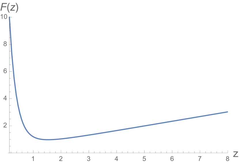
(a) Black hole line defined by equation (27).

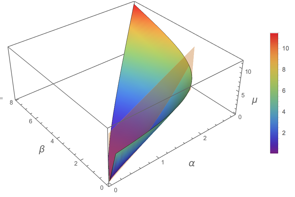
(b) Black hole surface $\mu=\mu(\alpha,\beta)$ and boundary condition surface $\beta=\alpha$. The color coding corresponds to the magnitude of $\mu$.

Figure 1: Black hole line and black hole surface for theories with potential (31).

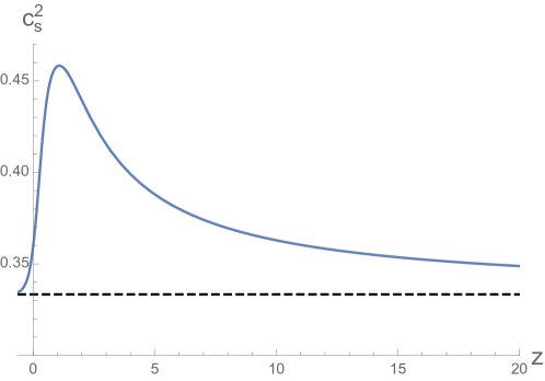
Figure 2: Speed of sound as a function of $z$ for the family of boundary conditions $\beta=\lambda\alpha$. The dashed line depicts the conformal value $c_{s}^{2}=1/3$, which is approached for large and small $z$.

For the linear boundary condition $\beta=\lambda\alpha$, we plot the speed of sound as a function of $z$ in Fig. 2 — for this deformation the energy density is obtained by replacing $W=\frac{\beta^{2}}{2\lambda}$ and $\alpha=\frac{\beta}{\lambda}$ in (20). This yields $\rho=\frac{\alpha^{2}l^{3}}{\kappa}\left(\frac{3}{2}F(z)-\frac{1}{8}\right)$. This is indeed an everywhere positive convex function for all the deformations we are considering. In the plots we have set $z=\frac{1}{2}\ln\left|\alpha\right|+1$. So, when $\alpha\gg 1$, then $z$ is very large and the deformed theory explores very high energies, where the conformal value for the speed of sound is recovered as one would expect. When $\alpha\sim 0$ then $z<0$ and the deformation vanishes. The conformal value for the speed of sound is again recovered in this limit. In the intermediate regime the speed of sound is larger than the conformal value, so it appears to be a very interacting state of matter which might be relevant for the description of neutron stars, where the speed of sound is believed to be bounded only by the speed of light [40]. We note that the conjectured bound ($c_{s}^{2}\leq 1/3$) for the speed of sound in theories with an holographic dual was only supposed to hold when there is no chemical potential [10]. This bound was indeed shown to be violated when a chemical potential is introduced in [11]. In this sense, this is the first example of the violation of the conjectured bound with an everywhere positive convex energy functional.

5 The Renormalization group

The field theory variables $\alpha$ and $\beta$ have an ambiguity when written in terms of the gravity variable $\varphi\,$, see (7). This is parametrized by the constant $r_{0}$ necessary to make the argument of the logarithm dimensionless. This is interpreted on the field theory side as a standard one-loop renormalization [26]. We take the bare coupling constant $\lambda_{\Lambda}$ and the bare field $\beta_{\Lambda}$ to be defined at the cutoff scale $\Lambda$ and the renormalized coupling constant $\lambda_{\nu}$ and renormalized field $\beta_{\nu}$ defined at the mass scale $\nu$. The independence of the bulk field from the renormalization procedure yields

$$\varphi l^{-4}=\frac{\beta_{\nu}\left(\lambda_{\nu}^{-1}\ln\left(r\nu\right)+1\right)}{r^{2}}+O(\frac{\ln(r)^{2}}{r^{3}})=\frac{\beta_{\Lambda}\left(\lambda_{\Lambda}^{-1}\ln\left(r\Lambda\right)+1\right)}{r^{2}}+O(\frac{\ln(r)^{2}}{r^{3}})$$ (33)

where the latter equality implies $\beta_{\nu}\lambda_{\nu}^{-1}=\beta_{\Lambda}\lambda_{\Lambda}^{-1}$ and $\lambda_{\nu}=\lambda_{\Lambda}+\ln\left(\Lambda/\nu\right)$ or alternatively

$$\lambda_{\nu}^{-1}=\frac{\lambda_{\Lambda}^{-1}}{1+\lambda_{\Lambda}^{-1}\ln\left(\Lambda/\nu\right)}\text{ ,}$$ (34)

which has the form of a one loop renormalization of a dimensionless coupling constant [26]. In the plot of the speed of sound of the previous section we have set $z=\frac{1}{2}\ln\left|\alpha\right|+1$, which means setting the renormalized coupling constant to one and measuring $\alpha$ in terms of the scale given by $\nu^{2}$:

$$z=\frac{1}{2}\ln\left|\frac{\alpha}{\nu^{2}}\right|+\lambda_{\nu}\text{ .}$$ (35)

The energy scale and the value of the dressed coupling constant are indeed necessary to compare the theoretical prediction with the experiment. A change in the values that we picked would imply a simple shift in the graph of figure 2.

6 Other scaling and spacetime dimensions

Although we have worked in five dimensions for scalar fields saturating the Breitenlohner-Freedman bound, our results are easily generalized to any spacetime dimension, $D$, for any scalar field with masses between this bound and the unitarity bound. Scalar fields with mass in the BF window (1) fall-off as

$$\varphi\sim\frac{\alpha}{r^{\Delta-}}+\frac{\beta}{r^{\Delta+}}+O(r^{-\Delta_{-}-1})\text{ ,}$$ (36)

where $2<\Delta_{-}<\Delta_{+}=D-1-\Delta_{-}$ and $\frac{\Delta_{+}}{\Delta_{-}}$ is not an integer [18]. The energy density is in these cases [19]

$$\rho\sim\frac{D-2}{2}\mu+\left(\Delta_{+}-\Delta_{-}\right)\left[W(\alpha)-\frac{\Delta_{-}}{D-1}\alpha\beta\right]\text{ ,}$$ (37)

where $\beta=\frac{dW\left(\alpha\right)}{d\alpha}$. Using the Smarr formula of [21] and the fact that $\rho-(D-2)p$ vanishes for AdS invariant boundary conditions yields

$$p\sim\frac{1}{2}\mu-\left(\Delta_{+}-\Delta_{-}\right)\left[W(\alpha)-\frac{\Delta_{-}}{D-1}\alpha\beta\right]\text{ .}$$ (38)

In these cases the black hole surface takes the form

$$\alpha=\alpha_{h}\left(\varphi_{h}\right)\mathcal{A}^{\frac{\Delta_{-}}{D-2}}\text{ ,}\qquad\mu\left(\varphi_{h},\mathcal{A}\right)=\mu_{h}\left(\varphi_{h}\right)\mathcal{A}^{\frac{D-1}{D-2}}\text{ ,}\qquad\beta=z\left(\varphi_{h}\right)\alpha^{\frac{\Delta_{+}}{\Delta-}}\text{ .}$$ (39)

and using the black hole line $\mu=F(z)\alpha^{\frac{D-1}{\Delta_{-}}}$ and the boundary condition $z=\omega(\alpha)$, the universal formula for the speed of sound is

$$c_{s}^{2}=\frac{1}{D-2}+2\frac{D-1}{D-2}\frac{\omega^{\prime}\alpha(D-1-2\Delta_{-})\Delta_{-}^{2}}{{(D-2)(D-1)}\left({(D-1)F+\omega^{\prime}\alpha\Delta}_{-}{\dot{F}}\right){-2\Delta_{-}^{2}(D-1-2\Delta}_{-}{)}\omega^{\prime}{\alpha}}.$$ (40)

which would allow one to model any given equation of state as for instance the one given by lattice QCD (for references see the recent review [41]). We shall provide a detailed derivation in a future work.

References

- [1] J. M. Maldacena, “The Large N limit of superconformal field theories and supergravity,” Adv. Theor. Math. Phys. 2 (1998) 231 [hep-th/9711200].
- [2] G. Policastro, D. T. Son and A. O. Starinets, “The Shear viscosity of strongly coupled N=4 supersymmetric Yang-Mills plasma,” Phys. Rev. Lett. 87 (2001) 081601 doi:10.1103/PhysRevLett.87.081601 [hep-th/0104066].
- [3] Y. Kats and P. Petrov, “Effect of curvature squared corrections in AdS on the viscosity of the dual gauge theory,” JHEP 0901 (2009) 044 doi:10.1088/1126-6708/2009/01/044 [arXiv:0712.0743 [hep-th]].
- [4] M. Brigante, H. Liu, R. C. Myers, S. Shenker and S. Yaida, “Viscosity Bound Violation in Higher Derivative Gravity,” Phys. Rev. D 77 (2008) 126006 doi:10.1103/PhysRevD.77.126006 [arXiv:0712.0805 [hep-th]].
- [5] U. Gursoy and E. Kiritsis, “Exploring improved holographic theories for QCD: Part I,” JHEP 0802 (2008) 032 doi:10.1088/1126-6708/2008/02/032 [arXiv:0707.1324 [hep-th]].
- [6] U. Gursoy, E. Kiritsis and F. Nitti, “Exploring improved holographic theories for QCD: Part II,” JHEP 0802 (2008) 019 doi:10.1088/1126-6708/2008/02/019 [arXiv:0707.1349 [hep-th]].
- [7] S. S. Gubser and A. Nellore, “Mimicking the QCD equation of state with a dual black hole,” Phys. Rev. D 78 (2008) 086007 doi:10.1103/PhysRevD.78.086007 [arXiv:0804.0434 [hep-th]].
- [8] S. S. Gubser, A. Nellore, S. S. Pufu and F. D. Rocha, “Thermodynamics and bulk viscosity of approximate black hole duals to finite temperature quantum chromodynamics,” Phys. Rev. Lett. 101 (2008) 131601 doi:10.1103/PhysRevLett.101.131601 [arXiv:0804.1950 [hep-th]].
- [9] S. He, Y. P. Hu and J. H. Zhang, “Hydrodynamics of a 5D Einstein-dilaton black hole solution and the corresponding BPS state,” JHEP 1112 (2011) 078 doi:10.1007/JHEP12(2011)078 [arXiv:1111.1374 [hep-th]].
- [10] A. Cherman, T. D. Cohen and A. Nellore, “A Bound on the speed of sound from holography,” Phys. Rev. D 80 (2009) 066003 doi:10.1103/PhysRevD.80.066003 [arXiv:0905.0903 [hep-th]].
- [11] C. Hoyos, N. Jokela, D. Rodríguez Fernández and A. Vuorinen, “Breaking the sound barrier in AdS/CFT,” Phys. Rev. D 94 (2016) no.10, 106008 doi:10.1103/PhysRevD.94.106008 [arXiv:1609.03480 [hep-th]].
- [12] P. Breitenlohner and D. Z. Freedman, “Positive Energy in anti-De Sitter Backgrounds and Gauged Extended Supergravity,” Phys. Lett. B 115 (1982) 197.
- [13] P. Breitenlohner and D. Z. Freedman, “Stability in Gauged Extended Supergravity,” Annals Phys. 144, 249 (1982).
- [14] T. Hertog and G. T. Horowitz, “Designer gravity and field theory effective potentials,” Phys. Rev. Lett. 94 (2005) 221301 doi:10.1103/PhysRevLett.94.221301 [hep-th/0412169].
- [15] H. S. Liu and H. Lü, “Scalar Charges in Asymptotic AdS Geometries,” Phys. Lett. B 730 (2014) 267 doi:10.1016/j.physletb.2014.01.056 [arXiv:1401.0010 [hep-th]].
- [16] A. Anabalon, D. Astefanesei and R. Mann, “Holographic equation of state in fluid/gravity duality,” arXiv:1604.05595 [hep-th].
- [17] A. Ishibashi and R. M. Wald, “Dynamics in nonglobally hyperbolic static space-times. 3. Anti-de Sitter space-time,” Class. Quant. Grav. 21 (2004) 2981 [hep-th/0402184].
- [18] M. Henneaux, C. Martinez, R. Troncoso and J. Zanelli, “Asymptotic behavior and Hamiltonian analysis of anti-de Sitter gravity coupled to scalar fields,” Annals Phys. 322 (2007) 824 [hep-th/0603185].
- [19] A. J. Amsel and D. Marolf, “Energy Bounds in Designer Gravity,” Phys. Rev. D 74 (2006) 064006 Erratum: [Phys. Rev. D 75 (2007) 029901] doi:10.1103/PhysRevD.74.064006, 10.1103/PhysRevD.75.029901 [hep-th/0605101].
- [20] A. Anabalon, D. Astefanesei and C. Martinez, “Mass of asymptotically anti de Sitter hairy spacetimes,” Phys. Rev. D 91, no. 4, 041501 (2015) doi:10.1103/PhysRevD.91.041501 [arXiv:1407.3296 [hep-th]].
- [21] H. S. Liu, H. Lu and C. N. Pope, “Generalized Smarr formula and the viscosity bound for Einstein-Maxwell-dilaton black holes,” Phys. Rev. D 92 (2015) 064014 doi:10.1103/PhysRevD.92.064014 [arXiv:1507.02294 [hep-th]].
- [22] A. Anabalon and D. Astefanesei, “On attractor mechanism of black holes,” Phys. Lett. B 727, 568 (2013) doi:10.1016/j.physletb.2013.11.013 [arXiv:1309.5863 [hep-th]].
- [23] A. Sen, “Black hole entropy function and the attractor mechanism in higher derivative gravity,” JHEP 0509, 038 (2005) doi:10.1088/1126-6708/2005/09/038 [hep-th/0506177].
- [24] A. Sen, “Black Hole Entropy Function, Attractors and Precision Counting of Microstates,” Gen. Rel. Grav. 40, 2249 (2008) doi:10.1007/s10714-008-0626-4 [arXiv:0708.1270 [hep-th]].
- [25] D. Astefanesei, K. Goldstein, R. P. Jena, A. Sen and S. P. Trivedi, “Rotating attractors,” JHEP 0610, 058 (2006) doi:10.1088/1126-6708/2006/10/058 [hep-th/0606244].
- [26] E. Witten, “Multitrace operators, boundary conditions, and AdS / CFT correspondence,” hep-th/0112258.
- [27] S. Kuperstein and A. Mukhopadhyay, “The unconditional RG flow of the relativistic holographic fluid,” JHEP 1111, 130 (2011) doi:10.1007/JHEP11(2011)130 [arXiv:1105.4530 [hep-th]].
- [28] S. Kuperstein and A. Mukhopadhyay, “Spacetime emergence via holographic RG flow from incompressible Navier-Stokes at the horizon,” JHEP 1311, 086 (2013) doi:10.1007/JHEP11(2013)086 [arXiv:1307.1367 [hep-th]].
- [29] M. Henningson and K. Skenderis, “The Holographic Weyl anomaly,” JHEP 9807, 023 (1998) doi:10.1088/1126-6708/1998/07/023 [hep-th/9806087].
- [30] V. Balasubramanian and P. Kraus, “A Stress tensor for Anti-de Sitter gravity,” Commun. Math. Phys. 208 (1999) 413 [hep-th/9902121].
- [31] R. B. Mann,“Misner string entropy,” Phys. Rev. D 60, 104047 (1999) [hep-th/9903229].
- [32] M. Bianchi, D. Z. Freedman and K. Skenderis, “How to go with an RG flow,” JHEP 0108 (2001) 041 doi:10.1088/1126-6708/2001/08/041 [hep-th/0105276].
- [33] M. Bianchi, D. Z. Freedman and K. Skenderis, “Holographic renormalization,” Nucl. Phys. B 631 (2002) 159 doi:10.1016/S0550-3213(02)00179-7 [hep-th/0112119].
- [34] D. Marolf and S. F. Ross, “Boundary Conditions and New Dualities: Vector Fields in AdS/CFT,” JHEP 0611 (2006) 085 doi:10.1088/1126-6708/2006/11/085 [hep-th/0606113].
- [35] I. Papadimitriou, “Multi-Trace Deformations in AdS/CFT: Exploring the Vacuum Structure of the Deformed CFT,” JHEP 0705 (2007) 075 [hep-th/0703152].
- [36] A. Anabalon, D. Astefanesei, D. Choque and C. Martinez, “Trace Anomaly and Counterterms in Designer Gravity,” JHEP 1603, 117 (2016) doi:10.1007/JHEP03(2016)117 [arXiv:1511.08759 [hep-th]].
- [37] R. C. Myers, “Stress tensors and Casimir energies in the AdS / CFT correspondence,” Phys. Rev. D 60 (1999) 046002 [hep-th/9903203].
- [38] E. Witten, “Anti-de Sitter space and holography,” Adv. Theor. Math. Phys. 2 (1998) 253 [hep-th/9802150].
- [39] D. Z. Freedman, S. S. Gubser, K. Pilch and N. P. Warner, “Continuous distributions of D3-branes and gauged supergravity,” JHEP 0007 (2000) 038 doi:10.1088/1126-6708/2000/07/038 [hep-th/9906194].
- [40] C. E. Rhoades, Jr. and R. Ruffini, “Maximum mass of a neutron star,” Phys. Rev. Lett. 32 (1974) 324. doi:10.1103/PhysRevLett.32.324
- [41] O. Philipsen, “The QCD equation of state from the lattice,” Prog. Part. Nucl. Phys. 70 (2013) 55 doi:10.1016/j.ppnp.2012.09.003 [arXiv:1207.5999 [hep-lat]].