Alignment of dynamic networks

Abstract

Motivation: Networks can model real-world systems in a variety of domains. Network alignment (NA) aims to find a node mapping that conserves similar regions between compared networks. NA is applicable to many fields, including computational biology, where NA can guide the transfer of biological knowledge from well- to poorly-studied species across aligned network regions. Existing NA methods can only align static networks. However, most complex real-world systems evolve over time and should thus be modeled as dynamic networks. We hypothesize that aligning dynamic network representations of evolving systems will produce superior alignments compared to aligning the systems’ static network representations, as is currently done.
Results: For this purpose, we introduce the first ever dynamic NA method, DynaMAGNA++. This proof-of-concept dynamic NA method is an extension of a state-of-the-art static NA method, MAGNA++. Even though both MAGNA++ and DynaMAGNA++ optimize edge as well as node conservation across the aligned networks, MAGNA++ conserves static edges and similarity between static node neighborhoods, while DynaMAGNA++ conserves dynamic edges (events) and similarity between evolving node neighborhoods. For this purpose, we introduce the first ever measure of dynamic edge conservation and rely on our recent measure of dynamic node conservation. Importantly, the two dynamic conservation measures can be optimized using any state-of-the-art NA method and not just MAGNA++. We confirm our hypothesis that dynamic NA is superior to static NA, under fair comparison conditions, on synthetic and real-world networks, in computational biology and social network domains. DynaMAGNA++ is parallelized and it includes a user-friendly graphical interface.
Software: Available upon request.
Supplementary information: Available upon request.
Contact: tmilenko@nd.edu, vvijayan@nd.edu

1 Introduction

Networks can be used to model complex real-world systems in a variety of domains (Boccaletti et al., 2006). Network alignment (NA) compares networks with the goal of finding a node mapping that conserves topologically or functionally similar regions between the networks. NA has been used in many domains and applications (Emmert-Streib et al., 2016). In computer vision, it has been used to find correspondences between sets of visual features (Duchenne et al., 2011). In online social networks, NA has been used to match identities of people who have different account types (e.g., Twitter and Facebook) (Zhang et al., 2015). In ontology matching, NA has been used to match concepts across ontological networks (Bayati et al., 2013). Computational biology is no exception. In this domain, NA has been used to predict protein function (including the role of proteins in aging), by aligning protein interaction networks (PINs) of different species, and by transferring functional knowledge from a well-studied species to a poorly-studied species between the species’ conserved (aligned) PIN regions (Faisal et al., 2015a, b; Elmsallati et al., 2016; Meng et al., 2016b; Guzzi and Milenković, 2017). Also, NA has been used to construct phylogenetic trees of species based on similarities of their PINs or metabolic networks (Kuchaiev et al., 2010; Kuchaiev and Pržulj, 2011).

NA methods can be categorized as local or global (Meng et al., 2016b; Guzzi and Milenković, 2017). Local NA typically finds highly conserved but consequently small regions among compared networks, and it results in a many-to-many node mapping. On the other hand, global NA typically finds a one-to-one node mapping between compared networks that results in large but consequently suboptimally conserved network regions. Clearly, each of local NA and global NA has its (dis)advantages (Meng et al., 2016b, a; Guzzi and Milenković, 2017). In this paper, we focus on global NA, but our ideas are applicable to local NA as well. Also, NA methods can be categorized as pairwise or multiple (Faisal et al., 2015b; Guzzi and Milenković, 2017; Vijayan and Milenković, 2016). Pairwise NA aligns two networks while multiple NA can align more than two networks at once. While multiple NA can capture conserved network regions between more networks than pairwise NA, which may lead to deeper biological insights compared to pairwise NA, multiple NA is computationally much harder than pairwise NA since the complexity of the NA problem typically increases exponentially with the number of networks. This is why in this paper we focus on pairwise NA, but our ideas can be extended to multiple NA as well. Henceforth, we refer to global and pairwise NA simply as NA.

Existing NA methods can only align static networks. This is because in many domains and applications, static network representations are often used to model complex real-world systems, independent of whether the systems are static or dynamic. However, most real-world systems are dynamic, as they evolve over time. Static networks cannot fully capture the temporal aspect of evolving systems. Instead, such systems can be better modeled as dynamic networks (Holme, 2015). For example, a complex system such as a social network evolves over time as friendships are made and lost. Static networks cannot model the changes in interactions between nodes over time, while dynamic networks can capture the times during which the friendships begin and end. Other examples of systems that can be more accurately represented as dynamic networks include communication systems, human or animal proximity interactions, ecological systems, and many systems in biology that evolve over time, including brain or cellular functioning. In particular, regarding the latter, while cellular functioning is dynamic, current computational methods (including all existing NA methods) for analyzing systems-level molecular networks, such as PINs, deal with the networks’ static representations. This is in part due to unavailability of experimental dynamic molecular network data, owing to limitations of biotechnologies for data collection. Yet, as more dynamic molecular (and other real-world) network data are becoming available, there is a growing need for computational methods that are capable of analyzing dynamic networks (Przytycka and Kim, 2010; Przytycka et al., 2010), including methods that can align such networks.

The question is: how to align dynamic networks, when the existing NA methods can only deal with static networks? To allow for this, we generalize the notion of static NA to its dynamic counterpart. Namely, we define dynamic NA as a process of comparing dynamic networks and finding similar regions between such networks, while exploiting the temporal information explicitly (unlike static NA, which ignores this information). We hypothesize that aligning dynamic network representations of evolving real-world systems will produce superior alignments compared to aligning the systems’ static network representations, as is currently done. To test this hypothesis, we introduce the first ever method for dynamic NA.

Our proposed dynamic NA method, DynaMAGNA++, is a proof-of-concept extension of a state-of-the-art static NA method, MAGNA++ (Vijayan et al., 2015). Saraph and Milenković (2014) and Vijayan et al. (2015) compared MAGNA++ to state-of-the-art static NA methods at the time, namely IsoRank (Singh et al., 2007), MI-GRAAL (Kuchaiev and Pržulj, 2011), and GHOST (Patro and Kingsford, 2012). More recently, Meng et al. (2016b) compared MAGNA++ to additional newer static NA methods: NETAL (Neyshabur et al., 2013), GEDEVO (Ibragimov et al., 2013), WAVE (Sun et al., 2015), and L-GRAAL (Malod-Dognin and Pržulj, 2015). The comparisons were made on synthetic as well as real-world PINs, in terms of both topological and functional alignment quality. MAGNA++ was found to be superior to six of the seven existing methods and comparable to the remaining method. This is exactly why we have chosen to extend MAGNA++ rather than some other static NA method to its dynamic counterpart. However, as any future static NA methods are developed (Hayes and Mamano, 2016) that are potentially superior to MAGNA++, our ideas on dynamic NA will be applicable to such methods too. Section 2 describes the method, and Section 3 confirms our hypothesis that dynamic NA is superior to static NA, under fair comparison conditions, on both synthetic and real-world networks, and on data from both computational biology and social network domains.

2 Methods

We first summarize MAGNA++, and then we describe our proposed dynamic NA method, DynaMAGNA++, as an extension of MAGNA++.

2.1 MAGNA++

Static networks and static NA. A static network $G(V,E)$ consists of a node set $V$ and an edge set $E$. An edge $(u,v)\in E$ is an interaction between nodes $u$ and $v$. There can only be a single edge between the same pair of nodes. Given two static networks $G_{1}(V_{1},E_{1})$ and $G_{2}(V_{2},E_{2})$, assuming without loss of generality that $|V_{1}|\leq|V_{2}|$, a static NA between $G_{1}$ and $G_{2}$ is a one-to-one node mapping $f\,\colon\,V_{1}\to V_{2}$, which produces the set of aligned node pairs $\{(v,f(v))\mid v\in V_{1}\}$ (Figure 1(a)).

Static edge conservation. Given an NA between two static networks, an edge in one network is conserved if it maps to an edge in the other network, and an edge in one network is non-conserved if it maps to a non-adjacent node pair (i.e., a non-edge) in the other network (Figure 1(a)). A good static NA is a node mapping that conserves similar network regions. That is, a good static NA should have a large number of conserved edges and a small number of non-conserved edges. In this context, we measure the quality of a static NA using the popular symmetric substructure score (S³) edge conservation measure (Saraph and Milenković, 2014).

S³ is defined as follows. Formally, the number of conserved edges is

$$N_{c}=\sum_{(u,v)\in V_{1}\otimes V_{1}}{\mathds{1}\left[(u,v)\in E_{1}\wedge(f(u),f(v))\in E_{2}\right]},$$

and the number of non-conserved edges is

$$\begin{split}N_{n}&=\sum_{(u,v)\in V_{1}\otimes V_{1}}\mathds{1}{[\,}((u,v)\in E_{1}\wedge(f(u),f(v))\notin E_{2})\,\,\,\vee\\[-8.0pt] &\,\,\,\,\,\qquad\qquad\qquad\,\,((u,v)\notin E_{1}\wedge(f(u),f(v))\in E_{2})\,]\\ &=\lvert E_{1}\rvert+\lvert E^{\prime}_{2}\rvert-2N_{c},\end{split}$$

where $G^{\prime}_{2}(V^{\prime}_{2},E^{\prime}_{2})$ is the subgraph of $G_{2}$ induced by $V^{\prime}_{2}=\{f(u)\mid u\in V_{1}\}$, $\mathds{1}\left[p\right]=1$ if $p$ is true and $\mathds{1}\left[p\right]=0$ if $p$ is false, and $U\otimes V$ is the Cartesian product of sets $U$ and $V$. Then,

$$\mbox{S}^{3}=\frac{N_{c}}{N_{c}+N_{n}}.$$

Our implementation of S³ that can compute this measure in $O(|E_{1}|+|E_{2}|)$ time complexity is described in the Supplement.

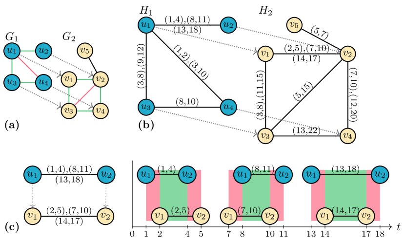
Figure 1: (a) Two static networks $G_{1}(V_{1},E_{1})$ and $G_{2}(V_{2},E_{2})$ (where edges between nodes in the same network are denoted by solid lines), and a static NA between them (in this case, $u_{i}$ maps to $v_{i}$ for $i=1,\ldots,4$, as shown by the dotted arrows). An edge is conserved if it maps to another edge (e.g., edge $(u_{1},u_{2})$ maps to edge $(v_{1},v_{2})$). An edge is non-conserved if it maps to a non-adjacent (disconnected) node pair (e.g., edge $(u_{1},u_{4})$ maps to a disconnected node pair $(v_{1},v_{4})$). All conserved edges are shown in green, and all non-conserved edges are shown in red. (b) Two dynamic networks $H_{1}(V_{1},T_{1})$ and $H_{2}(V_{2},T_{2})$. If two nodes interact at least once during the network’s lifetime (i.e., if there is at least one event between the nodes), there is a solid line between the nodes. A given solid line can capture multiple events. Each event is represented as $(t_{s},t_{e})$, where $t_{s}$ is its start time, and $t_{e}$ is its end time. For example, the event between $u_{3}$ and $u_{4}$ is active from start time 8 to end time 10. A dynamic NA is a node mapping between the two networks (in this case, $u_{i}$ maps to $v_{i}$ for $i=1,\ldots,4$, as shown by the dotted arrows).

Figure 2: (c) Illustration of the conserved event time (CET) and non-conserved event time (NCET) of the mapping of node pair $(u_{1},u_{2})$ to node pair $(v_{1},v_{2})$. On the left are node pair $(u_{1},u_{2})$ from dynamic network $H_{1}(V_{1},T_{1})$ and node pair $(v_{1},v_{2})$ from dynamic network $H_{2}(V_{2},T_{2})$, where $(u_{1},u_{2})$ maps to $(v_{1},v_{2})$. For each of the two node pairs $(u_{1},u_{2})$ and $(v_{1},v_{2})$, the event times of the given node pair are visualized by the plot on the right, where the given solid line in the plot indicates the start time to the end time of the given event (i.e., the period of time during which the given node pair is active). Given the above, the CET between $(u_{1},u_{2})$ and $(v_{1},v_{2})$ is the amount of time during which both $(u_{1},u_{2})$ and $(v_{1},v_{2})$ are active at the same time (the green area). Similarly, the NCET between $(u_{1},u_{2})$ and $(v_{1},v_{2})$ is the amount of time during which exactly one of $(u_{1},u_{2})$ or $(v_{1},v_{2})$ is active (the red area). We calculate the CET between these two illustrated node pairs as follows. Since the events $(u_{1},u_{2},1,4)$ and $(v_{1},v_{2},2,5)$ are both active from time 2 to time 4 for a duration of $4-2=2$, the events $(u_{1},u_{2},8,11)$ and $(v_{1},v_{2},7,10)$ are both active from time 8 to time 10 for a duration of $10-8=2$, and the events $(u_{1},u_{2},13,18)$ and $(v_{1},v_{2},14,17)$ are both active from time 14 to time 17 for a duration of $17-14=3$, the total CET between $(u_{1},u_{2})$ and $(v_{1},v_{2})$ is $2+2+3=7$. We calculate the NCET between these two illustrated node pairs as follows. We know that $(u_{1},u_{2})$ is active during time periods 1 to 4, 8 to 11, and 13 to 18, totaling a duration of $(4-1)+(11-8)+(18-13)=11$, and that $(v_{1},v_{2})$ is active during time periods 2 to 5, 7 to 10, and 14 to 17, totaling a duration of $(5-2)+(10-7)+(17-14)=9$. Since NCET is the amount of time during which $(u_{1},u_{2})$ is active, or $(v_{1},v_{2})$ is active, but not both, we need to add up the time during which either node pair is active, and subtract the time during which both node pairs are active (making sure to subtract twice to avoid double counting, because of the “but not both” constraint). Since the time during which both node pairs are active is the CET, the NCET between $(u_{1},u_{2})$ and $(v_{1},v_{2})$ is $11+9-2\times 7=6$.

Static node conservation. A good static NA should also conserve the similarity between aligned node pairs, i.e., node conservation. Node conservation accounts for similarities between all pairs of nodes across the two networks. Node similarity can be defined in a way that depends on one’s goal or domain knowledge. In this work, we use a node similarity measure that is based on graphlets, as follows.

Graphlets (in the static setting) are small, connected, induced subgraphs of a larger static network (Milenković and Pržulj, 2008). Graphlets can be used to describe the extended network neighborhood of a node in a static network via the node’s graphlet degree vector (GDV). The GDV generalizes the degree of the node, which counts how many edges are incident to the node, i.e., how many times the node touches an edge (where an edge is the only graphlet on two nodes), into the vector of graphlet degrees (i.e., GDV), which counts how many times the node touches each of the graphlets on up to $n$ nodes, accounting in the process for different topologically unique node symmetry groups (automorphism orbits) that might exist within the given graphlet. In this work, we use all graphlets with up to four nodes, which contain 15 automorphism orbits, when calculating the GDV of a node, per recommendations of the existing studies (Hulovatyy et al., 2015, 2014). Hence, the GDV of a node has 15 dimensions containing counts for the 15 orbits.

Given GDVs of all nodes in two static networks $G_{1}(V_{1},E_{1})$ and $G_{2}(V_{2},E_{2})$, where $x_{u}$ is the GDV of node $u$, we calculate similarity $s(u,v)$ between nodes $u\in V_{1}$ and $v\in V_{2}$ by relying on an existing GDV-based measure of node similarity that was used by Hulovatyy et al. (2015). The measure works as follows. First, to extract GDV dimensions that contain the most relevant information about the extended network neighborhood of the given node, the measure first reduces dimensionality of each GDV via principal component analysis (PCA). PCA is performed on the vector set $\{x_{w}\mid w\in V_{1}\cup V_{2}\}$, where as few as needed to account for at least 99% of variance in the vector set of the first $k$ PCA components are kept. Let us denote by $y_{u}$ the dimensionality-reduced vector of $x_{u}$ that contains the $k$ PCA components. Second, we define node similarity $s(u,v)$ as the cosine similarity between $y_{u}$ and $y_{v}$. Third, given a static NA $f$, we define our node conservation measure as $\sum_{u\in V_{1}}{\frac{s(u,f(u))}{\lvert V_{1}\rvert}}$.

Objective function and optimization process (also known as search strategy). MAGNA++ is a search-based algorithm that finds a static NA by directly maximizing both edge and node conservation. Namely, MAGNA++ maximizes the objective function $\alpha S_{E}+(1-\alpha)S_{N}$, where $S_{E}$ is the S³ measure of static edge conservation described above, $S_{N}$ is the graphlet-based measure of static node conservation described above, and $\alpha$ is a parameter between 0 and 1 that controls for the two measures. In several studies, it was shown that $\alpha$ of 0.5 yields the best results (Vijayan et al., 2015; Meng et al., 2016b), which is the $\alpha$ value we use in this study, unless otherwise noted. Given an initial population of random static NAs, MAGNA++ evolves the population of alignments over a number of generations while aiming to maximize its objective function. MAGNA++ then returns the alignment from the final generation that has the highest value of the objective function.

2.2 DynaMAGNA++

Dynamic networks. A dynamic network $H(V,T)$ consists of a node set $V$ and an event set $T$, where an event is a temporal edge (Figure 1(b)). An event is represented as a 4-tuple $(u,v,t_{s},t_{e})$, where nodes $u$ and $v$ interact from time $t_{s}$ to time $t_{e}$. An event $(u,v,t_{s},t_{e})\in T$ is active at time $t$ if $t_{s}\leq t\leq t_{e}$. The duration of an event is the time during which an event is active, i.e., $t_{e}-t_{s}$. There can be multiple events between the same two nodes in the dynamic network, but no two events between the same two nodes may be active at the same time. In fact, if there are two events between the same two nodes that are active at the same time, then they must be combined into a single event.

Above is the representation of a dynamic network that our study relies on. Sometimes, dynamic data is provided in a different dynamic network representation, most often as a discrete temporal sequence of static network snapshots $G_{1}(V_{1},E_{1}),\ldots,G_{k}(V_{k},E_{k})$. We can easily convert the static snapshot-based representation of a dynamic network into our event duration-based representation (i.e., into $H(V,T)$ as defined above). We do this as follows: if there is an edge connecting two nodes in the ${t}^{\textrm{th}}$ snapshot of the snapshot-based representation, then there is an event between the two nodes that is active from time $t$ to time $t+1$ in the event duration-based representation. In other words, we combine the node sets of the snapshots into a single node set $V=V_{1}\cup\ldots\cup V_{k}$. Then, for each snapshot $G_{t}$, $t=1,\ldots,k$, we convert each edge $(u,v)\in E_{t}$ into an event between nodes $u\in V$ and $v\in V$ in the dynamic network $H(V,T)$ with start time $t$ and end time $t+1$, i.e., the event $(u,v,t,t+1)$. This allows us to use the snapshot-based representation of a dynamic network in our study.

Dynamic NA. Given two dynamic networks $H_{1}(V_{1},T_{1})$ and $H_{2}(V_{2},T_{2})$, assuming without loss of generality that $|V_{1}|\leq|V_{2}|$, a dynamic NA between $H_{1}$ and $H_{2}$ is a one-to-one node mapping $f\,\colon\,V_{1}\to V_{2}$, which produces the set of aligned node pairs $\{(v,f(v))\mid v\in V_{1}\}$ (Figure 1(b)). Note the similarity between the definitions of static NA and dynamic NA (although the process of finding the actual alignments is different). This makes static NA and dynamic NA fairly comparable.

Dynamic edge (event) conservation. First, given node pair $(u_{1},u_{2})$ in $H_{1}$ that maps to node pair $(v_{1},v_{2})$ in $H_{2}$ (Figure 1(c)), we extend the notion of a conserved or non-conserved edge from static NA to dynamic NA by accounting for the amount of time that the mapping of $(u_{1},u_{2})$ to $(v_{1},v_{2})$ is conserved or non-conserved (defined below). That is, we extend the notion of a conserved or non-conserved static edge to the amount of a conserved or non-conserved dynamic edge (event), as follows.

Intuitively, we define the amount of a conserved event as follows. Similar to how an edge $(u^{\prime}_{1},u^{\prime}_{2})$ in static network $G_{1}(V_{1},E_{1})$ is conserved if it maps to an edge $(v^{\prime}_{1},v^{\prime}_{2})$ in static network $G_{2}(V_{2},E_{2})$ (and vice versa), the mapping of $(u_{1},u_{2})$ to $(v_{1},v_{2})$ is conserved at time $t$ if both $(u_{1},u_{2})$ and $(v_{1},v_{2})$ are active at time $t$. We refer to the entire amount of time during which this mapping is conserved as the conserved event time (CET) between $(u_{1},u_{2})$ and $(v_{1},v_{2})$. In other words, it is the amount of time during which both $(u_{1},u_{2})$ and $(v_{1},v_{2})$ are active at the same time. Formally, let $T_{u_{1}u_{2}}$ be the set of events between $u_{1}$ and $u_{2}$. Similarly, let $T_{v_{1}v_{2}}$ be the set of events between $v_{1}$ and $v_{2}$. Given this, the CET between $(u_{1},u_{2})$ and $(v_{1},v_{2})$ is

$$\begin{split}\mbox{CET}((u_{1},u_{2}),(v_{1},v_{2}))=\sum_{e\in T_{u_{1}u_{2}}}\sum_{e^{\prime}\in T_{v_{1}v_{2}}}ct(e,e^{\prime}),\\ \end{split}$$

where the conserved time $ct(e,e^{\prime})=\max(0,\min(t_{e},t^{\prime}_{e})-\max(t_{s},t^{\prime}_{s}))$ is the amount of time during which events $e=(u_{1},u_{2},t_{s},t_{e})$ and $e^{\prime}=(v_{1},v_{2},t^{\prime}_{s},t^{\prime}_{e})$ are active at the same time, i.e., $ct(e,e^{\prime})$ is the length of the overlap of the intervals $[t_{s},t_{e}]$ and $[t^{\prime}_{s},t^{\prime}_{e}]$.

Intuitively, we define the amount of a non-conserved event as follows. Similar to how an edge $(u^{\prime}_{1},u^{\prime}_{2})$ in $G_{1}$ is non-conserved if it maps to a disconnected node pair $(v^{\prime}_{1},v^{\prime}_{2})$ in $G_{2}$ (or vice versa), the mapping of $(u_{1},u_{2})$ to $(v_{1},v_{2})$ is non-conserved at time $t$ if exactly one of $(u_{1},u_{2})$ or $(v_{1},v_{2})$ is active at time $t$. We refer to the entire amount of time during which this mapping is non-conserved as the non-conserved event time (NCET) between $(u_{1},u_{2})$ and $(v_{1},v_{2})$. In other words, it is the amount of time during which $(u_{1},u_{2})$ is active, or $(v_{1},v_{2})$ is active, but not both are active at the same time. Formally, the NCET between $(u_{1},u_{2})$ and $(v_{1},v_{2})$ is

$$\mbox{NCET}((u_{1},u_{2}),(v_{1},v_{2}))=\sum_{e\in T_{u_{1}u_{2}}}d(e)+\sum_{e^{\prime}\in T_{v_{1}v_{2}}}d(e^{\prime})-2\sum_{e\in T_{u_{1}u_{2}}}\sum_{e^{\prime}\in T_{v_{1}v_{2}}}ct(e,e^{\prime}),$$

where $d(e)$ is the duration of event $e$, i.e., the amount of time during which $e$ is active. We make sure to subtract twice the amount of time during which $(u_{1},u_{2})$ and $(v_{1},v_{2})$ are both active due to the above “but not both are active at the same time” constraint.

Second, given the above definitions of CET and NCET between two node pairs $(u_{1},u_{2})$ and $(v_{1},v_{2})$, we extend the S³ measure of static node conservation to a new dynamic S³ (DS³) measure of dynamic edge (event) conservation, which we propose as a contribution of this study. To define DS³, we need to introduce the notion of CET between all node pairs across the entire alignment (rather than between just two aligned node pairs), henceforth simply referred to as alignment CET, which is the sum of CET between all node pair mappings between $H_{1}$ and $H_{2}$. Analogously, we need to define the notion of alignment NCET, which is the sum of NCET between all node pair mappings between $H_{1}$ and $H_{2}$. Alignment CET measures the amount of event conservation of the entire alignment and alignment NCET measures the amount of event non-conservation of the entire alignment. A good dynamic NA is a node mapping that conserves similar evolving network regions. That is, a good dynamic NA should have high alignment CET and low alignment NCET, which is what DS³ aims to capture. Formally, alignment CET is

$$T_{c}=\sum_{(u,v)\in V_{1}\otimes V_{1}}\mbox{CET}(\,(u,v),\,\,(f(u),f(v))\,)$$

and alignment NCET is

$$T_{n}=\sum_{(u,v)\in V_{1}\otimes V_{1}}\mbox{NCET}(\,(u,v),\,\,(f(u),f(v))\,).$$

Then,

$$\mbox{DS}^{3}=\frac{T_{c}}{T_{c}+T_{n}}.$$

Our implementation of DS³ that can compute this measure in $O(|T_{1}|+|T_{2}|)$ time complexity is described in the Supplement.

We note that there are many real-world networks that contain events with durations that are significantly less than the entire time window of the network, called “bursty” events. Examples of networks containing bursty events are e-mail communication networks, economic networks that model transactions, and brain networks constructed from oxygen level correlations as measured by fMRI scanning, each of whose events last much less than a second while the networks’ time windows span minutes to hours (Holme, 2015). Since bursty events are so short, small perturbations in the event times can greatly affect the resulting dynamic edge (event) conservation value. Thus, in order to allow our DS³ measure to be more robust to perturbations in the event times, one may simply extend the duration of each event in the network by some time $\Delta t$. Extending the duration of each event by $\Delta t$ will account for perturbations in event times of up to $\frac{\Delta t}{2}$ due to the following. Given two events $(u_{1},u_{2},t,t)$ and $(v_{1},v_{2},t^{\prime},t^{\prime})$ with durations of 0, where $t^{\prime}=t+\frac{\Delta t}{2}$, the conserved time $ct(\cdot,\cdot)$ between the two events is 0. Thus, if we want to consider the two events as conserved, we can increase the durations of both events by $\Delta t$ to create the modified events $(u_{1},u_{2},t,t+\Delta t)$ and $(v_{1},v_{2},t^{\prime},t^{\prime}+\Delta t)$, which results in a conserved time of $\frac{\Delta t}{2}$ for the two modified events. While we do not use this technique in our work since we do not use networks with bursty events, others might in the future, and if so, this needs to be considered when performing dynamic NA.

Dynamic node conservation. Just as for static NA, a good dynamic NA method should also conserve the similarity between aligned node pairs, i.e., node conservation. To take advantage of the temporal information encoded in dynamic networks that are being aligned and also to make dynamic NA as fairly comparable as possible to static NA, in this work, we rely on a measure of node similarity based on dynamic graphlets, as follows.

Dynamic graphlets are an extension of static graphlets (Section 2.1) from the static setting to the dynamic setting by accounting for temporal information in the dynamic network. While static graphlets can be used to capture the static extended network neighborhood of a node, dynamic graphlets can be used to capture how the extended neighborhood of a node changes over time. To describe dynamic graphlets formally, we first present the notion of a $\Delta t$-time-respecting path and a $\Delta t$-connected network. A $\Delta t$-time-respecting path is a sequence of events that connect two nodes such that for any two consecutive events in the sequence, the end time of the earlier event and the start time of the later event are within $\Delta t$ time of each other (i.e., are $\Delta t$-adjacent). A dynamic network is $\Delta t$-connected if for each pair of nodes in the network, there is a $\Delta t$-time-respecting path between the two nodes. Then, just as a static graphlet is an equivalence class of isomorphic connected subgraphs (Section 2.1), a dynamic graphlet is an equivalence class of isomorphic $\Delta t$-connected dynamic subgraphs, where two graphlets are equivalent if they both have the same relative temporal order of events. We use $\Delta t=1$ in this work, per recommendations by Hulovatyy et al. (2015). Just as the GDV of a node in a static network is a topological descriptor for the extended neighborhood the node, there exists the dynamic GDV (DGDV) of a node in a dynamic network, which describes how the extended neighborhood of a node changes over time. Specifically, just as the GDV of a node counts how many times the node touches each static graphlet at each of its automorphism orbits, the DGDV of a node counts how many times the node touches each dynamic graphlet at each of its orbits. Dynamic graphlets have a similar notion of orbits as static graphlets do, which now depend on both topological and temporal positions of a node within the dynamic graphlet. To make things comparable as fairly as possible to static NA, and per recommendations by Hulovatyy et al. (2015), in this work, we use dynamic graphlets with up to four nodes and six events, which contain 3,727 automorphism orbits, when calculating the DGDV of a node. Hence, the DGDV of a node has 3,727 dimensions containing counts for the 3,727 orbits.

Given the DGDVs of all nodes in two dynamic networks $H_{1}(V_{1},T_{1})$ and $H_{2}(V_{2},T_{2})$, we calculate similarity $s(u,v)$ between nodes $u\in V_{1}$ and $v\in V_{2}$, in the same way as in Section 2.1 (by relying on the PCA-based dimensionality reduction of all nodes’ DGVDs, computing cosine similarity between the dimensionality-reduced PCA vectors, and accounting for resulting cosine similarities between all pairs of nodes across the compared networks to obtain the total dynamic node conservation).

Objective function and optimization process (also known as search strategy). DynaMAGNA++ is a search-based algorithm that finds a dynamic NA by directly maximizing both dynamic edge (event) and node conservation. Namely, DynaMAGNA++ maximizes the objective function $\alpha S_{T}+(1-\alpha)S_{N}$, where $S_{T}$ is the DS³ measure of dynamic edge conservation described above, $S_{N}$ is the DGDV-based measure of dynamic node conservation described above, and $\alpha$ is a parameter between 0 and 1 that controls for the two measures. To make DynaMAGNA++ fairly comparable to MAGNA++, here we also use MAGNA++’s best $\alpha$ value of 0.5, unless otherwise noted. Given an initial population of random dynamic NAs, DynaMAGNA++ evolves the population of alignments over a number of generations while aiming to maximize its objective function. DynaMAGNA++ then returns the alignment from the final generation that has the highest value of the objective function.

Time complexity. To align two dynamic networks $H_{1}(V_{1},T_{1})$ and $H_{2}(V_{2},T_{2})$, DynaMAGNA++ evolves a population of $p$ alignments over $N$ generations. It does so by using its crossover function (see Saraph and Milenković (2014) for details) to combine pairs of parent alignments in the given population into child alignments, for each generation. For each generation, the dynamic edge (event) conservation, dynamic node conservation, and crossover of $O(p)$ alignments are calculated. Since dynamic edge conservation takes $O(|T_{1}|+|T_{2}|)$ to compute, dynamic node conservation takes $O(|V_{1}|)$ time to compute, crossover takes $O(|V_{2}|)$ time to compute, and $\lvert V_{1}\rvert\leq\lvert V_{2}\rvert$, the time complexity of DynaMAGNA++ is $O(Np|V_{2}|+Np(|T_{1}|+|T_{2}|))$. Note that the calculation of dynamic edge and dynamic node conservation in DynaMAGNA++ is parallelized. This allows DynaMAGNA++ to be run on multiple cores, which empirically results in close to liner speedup.

Other parameters. Given an initial population of dynamic NAs, DynaMAGNA++ evolves the population for up to a specified number of generations or until it reaches a stopping criterion. For each generation, DynaMAGNA++ keeps an elite fraction of alignments from the current generation’s population for the next generation’s population. In addition to the dynamic edge and node conservation measures, and the $\alpha$ parameter that controls for the contribution of the two measures, the remaining parameters of DynaMAGNA++ are (i) the initial population, (ii) the size of the population, (iii), the maximum number of generations, (iv) the elite fraction, and (v) the stopping criterion. For DynaMAGNA++, we use a population of 15,000 alignments initialized randomly, as in the original MAGNA++ paper, unless otherwise noted. We specify a maximum of 10,000 generations, since the alignments that we test all converge by 10,000 generations. The elite fraction is 0.5, as in the original MAGNA++ paper. The algorithm stops when the highest objective function value in the population has increased less than 0.0001 within the last 500 generations, since the alignments that we test do not increase by a significant amount after this point.

To fairly compare DynaMAGNA++ against MAGNA++, we aim to set the parameters of both methods to be as similar as possible. So, other than MAGNA++’s edge and node conservation measures, the remaining parameters of MAGNA++ are the same as for DynaMAGNA++. This way, any differences that we see between results of DynaMAGNA++ and results of MAGNA++ will be the consequence of the differences of the two methods’ edge and node conservation measures, i.e., of accounting for temporal information in the network with DynaMAGNA++ and ignoring this information with MAGNA++. In other words, any differences that we see between results of DynaMAGNA++ and results of MAGNA++ will fairly reflect differences between dynamic NA and static NA.

3 Results and discussion

Since there are no other dynamic NA methods to compare against, we compare DynaMAGNA++ to the next best option, namely its static NA counterpart. That is, we compare DynaMAGNA++ when it is used to align two dynamic networks, to MAGNA++ when it is used to align static versions of the two dynamic networks. By “static versions”, we mean that we “flatten” or “aggregate” a dynamic network into a static network that will have the same set of nodes as the dynamic network and a static edge will exist between two nodes in the static network if there is at least one event between the same two nodes in the dynamic network. This network aggregation simulates the common practice where network analysis of time-evolving systems is done in a static manner, by ignoring their temporal information (Hulovatyy et al., 2015; Holme, 2015).

We evaluate DynaMAGNA++ and MAGNA++ on synthetic and real-world dynamic networks, as described in the following sections. Note that there is no need to compare DynaMAGNA++ to any other static NA method besides MAGNA++, because MAGNA++ was recently shown in a systematic and comprehensive manner to be superior to seven other state-of-the-art static NA methods (Section 1). So, by transitivity, to demonstrate that dynamic NA is superior to static NA, it is sufficient to demonstrate that DynaMAGNA++ is superior to MAGNA++.

3.1 Evaluation using synthetic networks

Motivation. A good NA approach should be able to produce high-quality alignments between networks that are similar and low-quality alignments between networks that are dissimilar (Yaveroğlu et al., 2015). In this test on synthetic networks, “similar” means networks that originate from the same network model, and “dissimilar” means networks that originate from different network models. So, we refer to this test as network discrimination. Thus, in this section, we evaluate the network discrimination performance of DynaMAGNA++ and MAGNA++.

Data. We perform this evaluation on a set of biologically inspired synthetic networks. Specifically, we generate 20 dynamic networks using four biologically inspired network evolution models (or versions of the same model with different parameter values) that simulate the evolution of PINs, resulting in five networks per model (Hulovatyy et al., 2015). The four models we use are (i) GEO-GD with $p=0.3$, (ii) GEO-GD with $p=0.7$, (iii) SF-GD with $p=0.3$ and $q=0.7$, and (iv) SF-GD with $p=0.7$ and $q=0.6$, where GEO-GD is a geometric gene duplication model with probability cut-off and SF-GD is a scale-free gene duplication model (Pržulj et al., 2010). Hulovatyy et al. (2015) generalized the static versions of these models to their dynamic counterparts, and we rely on the same model networks as those used by Hulovatyy et al. (2015) (see their paper for details). The synthetic networks are represented as snapshots, with 1,000 nodes in each of the networks, an average of 24 snapshots per network, and an average of 162 edges per snapshot, where any variation in network sizes is caused by the different parameter values of the considered network models.

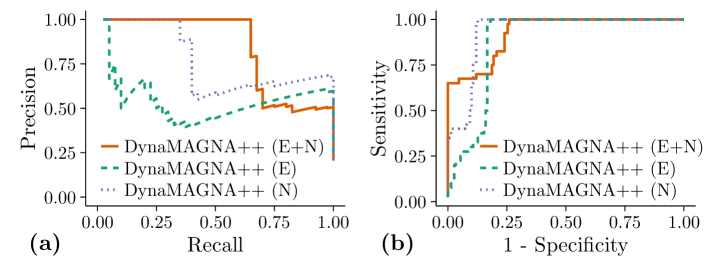
Figure 3: Network discrimination performance of DynaMAGNA++, while optimizing both dynamic edge and node conservation (E+N), dynamic edge conservation alone (E), and dynamic node conservation alone (N), for biological synthetic networks, with respect to (a) precision-recall curve and (b) ROC curve.

NA method	AUPR	F-score${}_{\mbox{cross}}$	F-score${}_{\mbox{max}}$	AUROC
DynaMAGNA++ (E+N)	0.836	0.675	0.788	0.928
DynaMAGNA++ (E)	0.551	0.400	0.750	0.878
DynaMAGNA++ (N)	0.770	0.625	0.808	0.934

Table 1: Network discrimination performance of DynaMAGNA++, while optimizing both dynamic edge and node conservation (E+N), dynamic edge conservation alone (E), and dynamic node conservation alone (N), for biological synthetic networks, with respect to the area under the precision-recall curve (AUPR), F-score at which precision and recall cross and are thus equal (F-score${}_{\mbox{cross}}$), maximum F-score (F-score${}_{\mbox{max}}$), and the area under the ROC curve (AUROC).

Evaluation measures. We calculate network discrimination performance of both methods as follows. We align all $20\choose 2$ pairs of the synthetic networks using DynaMAGNA++ and MAGNA++. The higher the alignment quality between pairs of similar networks (i.e., networks coming from the same model) and the lower the alignment between pairs of dissimilar networks (i.e., networks coming from different models), the better the NA method. Here, by alignment quality between two networks that the given method (DynaMAGNA++ or MAGNA++) identifies, we mean the method’s objective function value for the alignment of the two networks that is returned by the method (Section 2). For a given method, given all $20\choose 2$ alignment quality values, we summarize the method’s network discrimination performance using precision-recall and receiver operating characteristic (ROC) frameworks. Specifically, given the alignment quality values of all pairs of networks, for some given threshold $r$, a good NA method should result in alignment quality greater than $r$ for pairs of similar networks and in alignment quality smaller than $r$ for pairs of dissimilar networks. So, for a given threshold $r$, we compute accuracy in terms of precision, the fraction of network pairs that are similar and with alignment quality greater than $r$ out of all network pairs with alignment quality greater than $r$, and recall, the fraction of network pairs that are similar and with alignment quality greater than $r$ out of all similar network pairs. Varying the threshold $r$ for all $r\geq 0$ (i.e., for $r$ between 0 and the maximum observed alignment quality value, in increments of the smallest difference between any pair of observed alignment quality values) while plotting the resulting precision and recall values on the the $y$ and $x$ axes, respectively, gives us the precision-recall curve. Then, we compute the area under the precision-recall curve (AUPR), the F-score (harmonic mean of precision and recall) at which precision and recall cross and are thus equal (F-score${}_{\mbox{cross}}$), and the maximum F-score over all threshold $r$ values (F-score${}_{\mbox{max}}$). For a given threshold $r$, we also compute method accuracy in terms of sensitivity, which is the same as recall, and specificity, the fraction of network pairs that are dissimilar and with alignment quality less than $r$ out of all network pairs that are dissimilar. Varying the threshold $r$ for all $r\geq 0$ while plotting the resulting sensitivity and $1-$ specificity values on the the $y$ and $x$ axes, respectively, gives us the receiver operating characteristic (ROC) curve. Then, we compute the area under the ROC curve (AUROC).

Results. First, we aim to test whether optimizing both dynamic edge (event) conservation and dynamic node conservation in DynaMAGNA++ is better than optimizing either dynamic edge conservation alone or dynamic node conservation alone, since it was shown for MAGNA++ in previous studies that optimizing both static edge conservation and static node conservation performs better than optimizing either static edge conservation alone or static node conservation alone (Vijayan et al., 2015; Meng et al., 2016b). So, we compare three different versions of DynaMAGNA++ that differ in their optimization functions. Namely, the three versions optimize: (i) a combination of dynamic edge conservation and dynamic node conservation (corresponding to $\alpha=0.5$, named DynaMAGNA++ (E+N)), (ii) dynamic edge conservation only (corresponding to $\alpha=1$, named DynaMAGNA++ (E)), and (iii) dynamic node conservation only (corresponding to $\alpha=0$, named DynaMAGNA++ (N)) (Section 2). We find that overall DynaMAGNA++ (E+N) performs better than DynaMAGNA++ (E) and DynaMAGNA++ (N) (Figure 3 and Table 3.1), especially in terms of AUPR (as well as F-score${}_{\mbox{cross}}$), which is more credible than AUROC when there is an imbalance between the number of similar pairs and dissimilar pairs, as is the case in our study. So, henceforth, in the main paper, we only report results for DynaMAGNA++ (E+N) and refer to it simply as DynaMAGNA++. We report corresponding results for DynaMAGNA++ (E) and DynaMAGNA++ (N) in the Supplement. Thus, we fairly compare DynaMAGNA++ and MAGNA++, both using the $\alpha$ parameter value of 0.5.

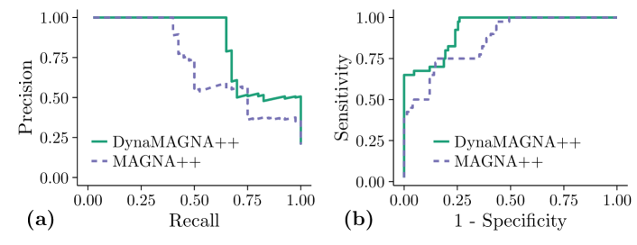
Figure 4: Network discrimination performance of DynaMAGNA++ and MAGNA++ for biological synthetic networks with respect to (a) precision-recall curve and (b) ROC curve.

Table 2: Network discrimination performance of DynaMAGNA++ and MAGNA++, for biological synthetic networks, with respect to the same measures as in Table 3.1.

Second, and most importantly, we aim to answer whether dynamic NA is better than static NA, by comparing the network discrimination performance of DynaMAGNA++ and MAGNA++. We find that DynaMAGNA++ performs better than MAGNA++ in the task of network discrimination with respect to all considered measures of NA quality (Figure 4 and Table 3.1; also, see the Supplement).

To illustrate generalizability of dynamic NA to other domains, we also evaluate the performance of DynaMAGNA++ and MAGNA++ on synthetic networks under a social network evolution model. We find that similar results (superiority of DynaMAGNA++ over MAGNA++) hold for the synthetic social networks as well (see the Supplement).

In summary, under fair comparison conditions, we demonstrate that dynamic NA is superior to static NA for synthetic dynamic networks.

3.2 Evaluation using real-world networks

Motivation. Here, we still evaluate whether the given method produces high-quality alignments for similar networks and low-quality alignments for dissimilar networks. However, here, for real-world networks, the notion of similarity that we use is different than for the synthetic networks above, because for real-world networks, we do not know which network models they belong to (Yaveroğlu et al., 2015). Specifically, here, we align an original real-world network to randomized (noisy) versions of the original network (see below), where we vary the noise level. The larger the noise level, the more dissimilar the aligned networks are, and consequently, the lower the alignment quality should be.

Zebra network. Since there is a lack of available dynamic molecular networks (Section 1), we begin our evaluation of real-world networks on an alternative biological network type, namely an ecological network. The original real-world network that we use is the Grevy’s zebra proximity network (Rubenstein et al., 2015), which contains information on interactions between 27 zebras in Kenya over 58 days. The data was collected by driving a predetermined route each day while searching for herds. There are 779 events in the network. We also report results for another animal proximity network that contains information on interactions between 28 onagers, a species that is closely related to the Grevy’s zebra, mostly in the Supplement. The onager proximity network contains 28 nodes and 522 events.

Since the difference between dynamic NA and static NA is that the former accounts for the temporal aspect of the data more explicitly than the latter, to properly validate results for dynamic NA, as strict randomization scheme as possible should be used when creating randomized (noisy) versions of the original dynamic network that will be aligned to the original network. By “as strict as possible”, we mean that we want to use a randomization scheme that preserves as much structure (i.e., topology) as possible of the dynamic network and randomizes only the temporal aspect of the network. This way, the only difference observed between DynaMAGNA++’s and MAGNA++’s performance will be the consequence of considering the temporal aspect of the data. For this reason, we randomize the original network using the following model per recommendations by Holme (2015). In order to randomize the original dynamic network $H(V,T)$ to a noise level, first, we arbitrarily number all $m$ events in the network as $T=\{e_{1},e_{2},\ldots,e_{m}\}$. Then, for each event $e_{i}$, with probability $p$ (where $p$ is the noise level) we randomly select another event $e_{j},j\neq i$, and swap the time stamps of the two events. Since we only swap the time stamps, this randomization scheme conserves the total number of events and the structure of the flattened version of the original dynamic network. We study 10 different noise levels (from 0% to 100% in smaller increments initially and larger increments toward the end). For each noise level, we generate five randomized versions of the original network and report results averaged over the five randomization runs.

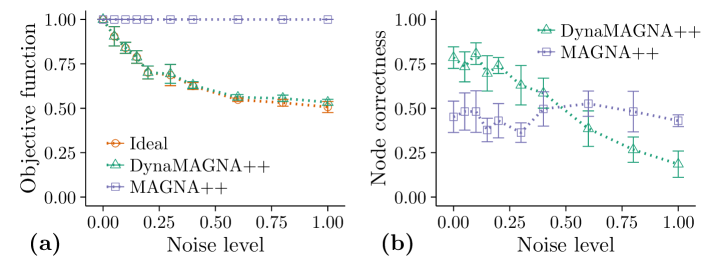
Figure 5: Alignment quality of DynaMAGNA++ and MAGNA++ as a function of noise level when aligning the original Grevy’s zebra network to randomized (noisy) versions of the original network. In this figure, the randomization is as strict as possible, as it conserves all structure of the flattened version of the original dynamic network and only randomly “shuffles” the given percentage (noise level) of its event time stamps. Alignment quality is shown with respect to (a) each method’s objective function, and (b) node correctness. “Ideal” in panel (a) shows the quality of perfect alignments, with respect to DynaMAGNA++’s objective function.

We evaluate DynaMAGNA++ and MAGNA++’s performance as follows. First, for a good method, alignment quality should decrease as the noise level increases, since the original network and its randomized version become more dissimilar with this increase. As in Section 3.1, one measure of alignment quality that we use is each method’s objective function. Another measure that we use is node correctness. Node correctness of an alignment is the fraction of correctly aligned node pairs (according to the ground truth node mapping) out of all aligned node pairs. Given that our original network and its randomized versions have the same set of nodes, we know which nodes in the original network correspond to which nodes in the given randomized network. That is, we know the ground truth mapping between the aligned networks (which henceforth we refer to as the perfect mapping). Hence, we can measure node correctness between the networks. Thus, we evaluate each method’s alignment quality using the method’s objective function as well as node correctness, with the expectation that for a good method, alignment quality should decrease with increase in the noise level.

Second, since we know the perfect alignment between the original network and each of its randomized versions, we compute the “ideal” alignment quality, i.e., the quality of the perfect alignment, as measured by DynaMAGNA++’s objective function. Here, the expectation is that a good method’s alignment quality should mimic well the quality of the perfect alignment.

Third, we expect DynaMAGNA++’s alignment quality to be superior to MAGNA++’s alignment quality with respect to node correctness for lower (meaningful) noise levels, if it is indeed true that dynamic NA is superior to static NA. We do not expect this superiority for higher noise levels, since at such noise levels, networks being aligned are highly randomized and thus a good method should produce low-quality alignments.

Indeed, our results confirm all three of the above expectations (Figure 5; also, see the Supplement). Specifically, first, DynaMAGNA++’s alignment quality indeed decreases with the increase in the noise level with respect to both its objective function (Figure 5(a)) as well as node correctness (Figure 5(b)). On the other hand, MAGNA++’s alignment quality stays constant with increase in the noise level. In other words, MAGNA++ produces alignments of the same quality for low noise levels (where network structure is meaningful) as it does for high noise levels (where network structure is random). Second, DynaMAGNA++’s alignment quality follows closely the quality of the perfect alignments (while MAGNA++ does not) (Figure 5(a)). Third, DynaMAGNA++ achieves higher node correctness than MAGNA++ at lower (meaningful) noise levels. This is not a surprise, since DynaMAGNA++ explicitly uses the temporal information in the aligned networks, while MAGNA++ does not. Thus, in summary, dynamic NA outperforms static NA. We observe similar results for the onager network (see the Supplement).

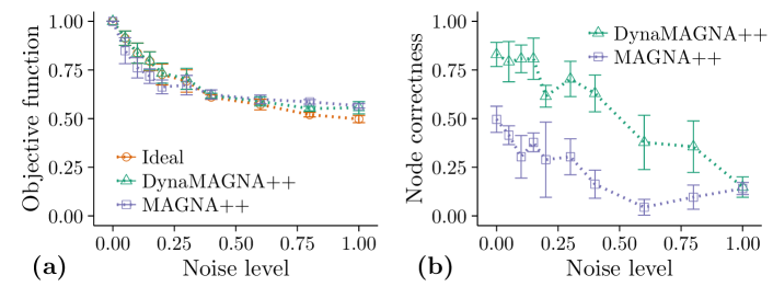
Figure 6: Alignment quality of DynaMAGNA++ and MAGNA++ for the Grevy’s zebra network. The figure can be interpreted in the same way as Figure 5, except that here, the randomization used to create the noisy networks does not conserve the structure of the flattened version of the original dynamic network.

The above complete failure of MAGNA++ to produce alignments of decreasing quality as the noise level increases is due to the strict randomization scheme that we use to create the noisy versions of the original network, which conserves all structure of the flattened version of the original dynamic network. Recall that we use the strict randomization scheme to ensure that the results of DynaMAGNA++ are meaningful. Yet, to give as fair advantage as possible to static NA, we produce a different set of noisy versions of the original network using somewhat more flexible randomization scheme that does not conserve the structure of the flattened version of the original dynamic network, per recommendations of Holme (2015). This randomization scheme works as follows. In order to randomize the original dynamic network $H(V,T)$ to a certain noise level, first, we arbitrarily number all $m$ events in the network as $T=\{e_{1},e_{2},\ldots,e_{m}\}$. Then, for each event $e_{i}$, with probability $p$ (where $p$ is the noise level) we randomly select an event $e_{i^{\prime}}$, and we rewire the two events. That is, given $e_{i}=(u,v,t_{s},t_{e})$ and $e_{i^{\prime}}=(u^{\prime},v^{\prime},t^{\prime}_{s},t^{\prime}_{e})$, we either set $e_{i}=(u,v^{\prime},t_{s},t_{e})$ and $e_{i^{\prime}}=(u^{\prime},v,t_{s},t_{e})$ with probability 0.5, or we set $e_{i}=(u,u^{\prime},t_{s},t_{e})$ and $e_{i^{\prime}}=(v,v^{\prime},t_{s},t_{e})$ with probability 0.5. If the rewiring creates a loop (i.e., an event from a node to itself) or multiple link (i.e., duplicate events between the same nodes), then we undo it and randomly select another event $e_{i^{\prime}}$. This randomization scheme conserves the entire set of time stamps of the original network, but it does not preserve the structure of the flattened network. We study 10 different noise levels (from 0% to 100% in smaller increments initially and larger increments toward the end). For each noise level, we generate five randomized versions of the original network and report results averaged over the five randomization runs. While now MAGNA++’s alignment quality also decreases with increase in the noise level and also MAGNA++ closely follows the quality of the perfect alignments, as it should (Figure 7(a); also, see the Supplement), DynaMAGNA++ is still superior to MAGNA++ with respect to node correctness (Figure 7(b)), which again implies that dynamic NA is superior to static NA.

Because the results are consistent independent of the randomization scheme that is used to produce noisy networks, and since the strict scheme should be used to correctly evaluate DynaMAGNA++’s correctness, henceforth, we report results only for the strict randomization scheme.

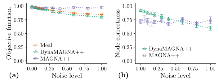
Figure 7: Alignment quality of DynaMAGNA++ and MAGNA++ for the yeast network. The figure can be interpreted in the same way as Figure 5.

Yeast network. Since there is a lack of available experimental dynamic molecular networks, we continue our evaluation of real-world networks on the next best available dynamic molecular network option. Namely, we create a dynamic yeast PIN from an artificial temporal sequence of static yeast PINs. Here, the static PINs that are used as snapshots of the dynamic PIN are are all real-world networks, it is just their temporal sequence that is artificial. The sequence consists of six static PIN snapshots: a high-confidence S. cerevisiae (yeast) PIN with 1,004 proteins and 8,323 interactions, and five lower-confidence yeast PINs constructed by adding to the high-confidence PIN 5%, 10%, 15%, 20%, or 25% of lower-confidence interactions; the higher-scoring lower-confidence interactions are added first. Clearly, the five lower-confidence PINs have the same 1,004 nodes as the high-confidence PIN, and the largest of the five lower-confidence PINs has 25% more edges than the high-confidence PIN, i.e., 10,403 of them. This network set has been used in many existing static NA studies (Kuchaiev et al., 2010; Milenković et al., 2010; Kuchaiev and Pržulj, 2011; Saraph and Milenković, 2014; Meng et al., 2016b; Vijayan and Milenković, 2016). When we use the six static PINs as snapshots to form a dynamic network, we order the six networks from the smallest one in terms of the number of edges (i.e., one of the highest confidence) to the largest one in terms of the number of edges (i.e., one of the lowest confidence). Since each static PIN contains the same set of nodes, this simulates a dynamic network that is growing as it evolves, with more and more interactions being added to the network over time. When we align the resulting (original) dynamic yeast network to its randomized versions, we find that just as for the zebra network, DynaMAGNA++’s alignment quality decreases with increase in the noise level, with respect to both its objective function (Figure 7(a)) as well as node correctness (Figure 7(b)), while MAGNA++’s alignment quality does not change. Further, DynaMAGNA++ again matches more closely the quality of the perfect alignments than MAGNA++ does with respect to DynaMAGNA++’s objective function (Figure 7(a)). Finally, DynaMAGNA++ produces higher node correctness than MAGNA++ for the lower (meaningful) noise levels. Thus, dynamic NA is superior to static NA for the yeast network as well.

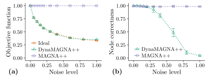
Figure 8: Alignment quality of DynaMAGNA++ and MAGNA++ for the Enron network. The figure can be interpreted in the same way as Figure 5.

Enron network. To demonstrate DynaMAGNA++’s generalizability on non-biological networks, we continue our evaluation of real-world networks on a social network. The original network that we use is the Enron e-mail communication network (Priebe et al., 2005), which is based on e-mail communications of 184 employees in the Enron corporation from 2000 to 2002, made public by the Federal Energy Regulatory Commission during its investigation. The entire two-year time period is divided into two-month periods so that if there is at least one e-mail sent between two people within a particular two-month period, then there exists an event between the two people during that period. There are 5,539 events in the Enron network. When we align the original network to its randomized versions, we find that just as for the zebra and yeast networks, DynaMAGNA++’s alignment quality decreases with increase in the noise level, while MAGNA++’s alignment quality does not change (Figure 8). Further, DynaMAGNA++ again matches more closely the quality of the perfect alignments (Figure 7(a)). So, these results again indicate that dynamic NA is superior to static NA. Interestingly, for this network, MAGNA++ also produces high-quality alignments with respect to node correctness for the low noise levels, just like DynaMAGNA++ does.

Running time. Recall that the time complexity of DynaMAGNA++ is linear with respect to the number of events in the aligned networks (Section 2.2), while the time complexity of MAGNA++ is linear with respect to the number of edges in the aligned networks (Section 2.1). Because there are typically far more events in a typical dynamic networks than edges in the flattened version of the dynamic network, and due to the more involved computations when calculating event conservation, DynaMAGNA++ is expected to be slower than MAGNA++ (yet, it is this ability of DynaMAGNA++ to capture detailed temporal event information that makes it superior to MAGNA++ in terms of accuracy). A representative runtime for DynaMAGNA++ and MAGNA++ when the methods are run on eight cores to align the yeast network to its 0% randomized version are 1.9 hours and 0.7 hours, respectively, which makes DynaMAGNA++ 2.7 times slower than MAGNA++. Yet, this somewhat slower (yet still very practical) runtime of DynaMAGNA++ is justified by DynaMAGNA++’s superiority over MAGNA++ in terms of alignment quality.

DynaMAGNA++’s availability. We implement a friendly graphical user interface (GUI) for DynaMAGNA++ (Figure 9) for easy use by domain (e.g., biological) scientists. Also, we provide the source code of DynaMAGNA++ so that computational scientists may potentially extend the work (available upon request).

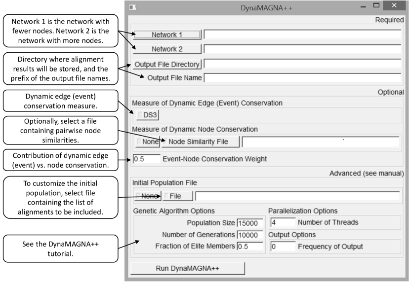
Figure 9: GUI to DynaMAGNA++. The only required parameters are the two networks to be aligned, and the output directory/file name information. While DS³ is the only currently implemented dynamic edge (event) conservation measure, other future dynamic edge conservation measures can be easily added. Any dynamic node similarity measure can be used by selecting a file containing pairwise similarities between nodes of the two networks. The $\alpha$ parameter (Section 2.2) can be set to any desired value. Other advanced parameters can also be user-specified. The default values are set according to the parameter values used in this work (Section 2.2).

4 Conclusion

We introduce the first ever dynamic NA method. We show that our method, DynaMAGNA++, produces superior alignments compared to its static NA counterpart due its explicit use of available temporal information in dynamic network data. DynaMAGNA++ is a search-based NA method that can optimize any alignment quality measure. In this work, we propose an efficient temporal information-based alignment quality measure, DS³, that DynaMAGNA++ optimizes in order to find good alignments. DynaMAGNA++ can be extended in two ways: by optimizing future, potentially more efficient alignment quality measures with the current search strategy, or by optimizing its current alignment quality measures with a future, potentially superior search strategy (Crawford et al., 2015).

We demonstrate applicability of DynaMAGNA++ and dynamic NA in general in multiple domains: biological networks (ecological networks and PINs) and social networks. Given the impact that static NA has had in computational biology, as more PIN and other molecular dynamic network data are becoming available, dynamic NA and thus our study will continue to gain importance. The same holds for other domains in which increasing amounts of real-world dynamic network data are being collected. So, we have just scratched the tip of the iceberg called dynamic NA.

Funding:

This work was supported by the National Science Foundation (NSF) [CCF-1319469] and the Air Force Office of Scientific Research (AFOSR) [YIP FA9550-16-1-0147].

References

- Bayati et al. (2013) Bayati, M., Gerritsen, M., Gleich, D., Saberi, A., and Wang, Y. (2013). Message-passing algorithms for sparse network alignment. ACM Trans. Knowl. Discov. Data, 7(1), 3:1–3:31.
- Boccaletti et al. (2006) Boccaletti, S., Latora, V., Moreno, Y., Chavez, M., and Hwang, D.-U. (2006). Complex networks: structure and dynamics. Phys. Rep., 424(4–5), 175 – 308.
- Crawford et al. (2015) Crawford, J., Sun, Y., and Milenković, T. (2015). Fair evaluation of global network aligners. Algorithms for Molecular Biology, 10(19).
- Duchenne et al. (2011) Duchenne, O., Bach, F., Kweon, I.-S., and Ponce, J. (2011). A tensor-based algorithm for high-order graph matching. Pattern Analysis and Machine Intelligence, IEEE Transactions on, 33(12), 2383–2395.
- Elmsallati et al. (2016) Elmsallati, A., Clark, C., and Kalita, J. (2016). Global alignment of protein-protein interaction networks: A survey. IEEE/ACM Trans. on Computational Biology and Bioinformormatics, 13(4), 689–705.
- Emmert-Streib et al. (2016) Emmert-Streib, F., Dehmer, M., and Shi, Y. (2016). Fifty years of graph matching, network alignment and network comparison. Info. Sciences, 346(C), 180–197.
- Faisal et al. (2015a) Faisal, F., Zhao, H., and Milenković, T. (2015a). Global network alignment in the context of aging. IEEE/ACM Transactions on Computational Biology and Bioinformatics, 12(1), 40–52.
- Faisal et al. (2015b) Faisal, F., Meng, L., Crawford, J., and Milenković, T. (2015b). The post-genomic era of biological network alignment. EURASIP Journal on Bioinformatics and Systems Biology, 2015(1), 1–19.
- Guzzi and Milenković (2017) Guzzi, P. H. and Milenković, T. (2017). Survey of local and global biological network alignment: the need to reconcile the two sides of the same coin. Briefings in Bioinformatics, doi: 10.1093/bib/bbw132.
- Hayes and Mamano (2016) Hayes, W. and Mamano, N. (2016). SANA: Simulated annealing network alignment applied to biological networks. arXiv, arXiv:1607.02642 [q-bio.MN].
- Holme (2015) Holme, P. (2015). Modern temporal network theory: a colloquium. The European Physical Journal B, 88(9), 1–30.
- Hulovatyy et al. (2014) Hulovatyy, Y., Solava, R. W., and Milenković, T. (2014). Revealing missing parts of the interactome via link prediction. PLOS ONE, 9(3), e90073.
- Hulovatyy et al. (2015) Hulovatyy, Y., Chen, H., and Milenković, T. (2015). Exploring the structure and function of temporal networks with dynamic graphlets. Bioinformatics, 31(12), 171–180.
- Ibragimov et al. (2013) Ibragimov, R., Malek, M., and Baumbach, J. (2013). GEDEVO: An evolutionary graph edit distance algorithm for biological network alignment. In GCB, pages 68–79.
- Kuchaiev and Pržulj (2011) Kuchaiev, O. and Pržulj, N. (2011). Integrative network alignment reveals large regions of global network similarity in yeast and human. Bioinformatics, 27(10), 1390–1396.
- Kuchaiev et al. (2010) Kuchaiev, O., Milenković, T., Memišević, V., Hayes, W., and Pržulj, N. (2010). Topological network alignment uncovers biological function and phylogeny. Journal of The Royal Society Interface, 7(50), 1341–1354.
- Malod-Dognin and Pržulj (2015) Malod-Dognin, N. and Pržulj, N. (2015). L-GRAAL: Lagrangian graphlet-based network aligner. Bioinformatics, 31(13), 2182–2189.
- Meng et al. (2016a) Meng, L., Crawford, J., Striegel, A., and Milenković, T. (2016a). IGLOO: Integrating global and local biological network alignment. In Proc. of Workshop on Mining and Learning with Graphs (MLG) at the Conference on Knowledge Discovery and Data Mining (KDD).
- Meng et al. (2016b) Meng, L., Striegel, A., and Milenković, T. (2016b). Local versus global biological network alignment. Bioinformatics, 32(20), 3155–3164.
- Milenković and Pržulj (2008) Milenković, T. and Pržulj, N. (2008). Uncovering biological network function via graphlet degree signatures. Cancer Informatics, 6, 257–273.
- Milenković et al. (2010) Milenković, T., Ng, W., Hayes, W., and Pržulj, N. (2010). Optimal network alignment with graphlet degree vectors. Cancer Informatics, 9, 121–137.
- Neyshabur et al. (2013) Neyshabur, B., Khadem, A., Hashemifar, S., and Shahriar Arab, S. (2013). NETAL: a new graph-based method for global alignment of protein-protein interaction networks. Bioinformatics, 29(13), 1654–1662.
- Patro and Kingsford (2012) Patro, R. and Kingsford, C. (2012). Global network alignment using multiscale spectral signatures. Bioinformatics, 28(23), 3105–3114.
- Priebe et al. (2005) Priebe, C. E., Conroy, J. M., Marchette, D. J., and Park, Y. (2005). Scan statistics on Enron graphs. Comput. Math. Organ. Theory, 11(3), 229–247.
- Pržulj et al. (2010) Pržulj, N., Kuchaiev, O., Stevanović, A., and Hayes, W. (2010). Geometric evolutionary dynamics of protein interaction networks. In Proc. of the Pacific Symposium Biocomputing, pages 4–8.
- Przytycka and Kim (2010) Przytycka, T. M. and Kim, Y.-A. (2010). Network integration meets network dynamics. BMC Bioinformatics, 8(48).
- Przytycka et al. (2010) Przytycka, T. M., Singh, M., and Slonim, D. K. (2010). Toward the dynamic interactome: it’s about time. Briefings in Bioinformatics, 11(1), 15–29.
- Rubenstein et al. (2015) Rubenstein, D. I., Sundaresan, S. R., Fischhoff, I. R., Tantipathananandh, C., and Berger-Wolf, T. Y. (2015). Similar but different: dynamic social network analysis highlights fundamental differences between the fission-fusion societies of two equid species, the onager and Grevy’s zebra. PLOS ONE, 10(10), e0138645.
- Saraph and Milenković (2014) Saraph, V. and Milenković, T. (2014). MAGNA: Maximizing accuracy in global network alignment. Bioinformatics, 30(20), 2931–2940.
- Singh et al. (2007) Singh, R., Xu, J., and Berger, B. (2007). Pairwise global alignment of protein interaction networks by matching neighborhood topology. In Research in computational molecular biology, pages 16–31. Springer.
- Sun et al. (2015) Sun, Y., Crawford, J., Tang, J., and Milenković, T. (2015). Simultaneous optimization of both node and edge conservation in network alignment via WAVE. In Proc. of Workshop on Algorithms in Bioinformatics (WABI), pages 16–39.
- Vijayan and Milenković (2016) Vijayan, V. and Milenković, T. (2016). Multiple network alignment via multiMAGNA++. In Proc. of Workshop on Data Mining in Bioinformatics (BIOKDD) at the Conference on Knowledge Discovery and Data Mining (KDD).
- Vijayan et al. (2015) Vijayan, V., Saraph, V., and Milenković, T. (2015). MAGNA++: Maximizing Accuracy in Global Network Alignment via both node and edge conservation. Bioinformatics, 31(14), 2409–2411.
- Yaveroğlu et al. (2015) Yaveroğlu, Ö., Milenković, T., and Prz̆ulj (2015). Proper evaluation of alignment-free network comparison methods. Bioinformatics, 31(16), 2697–2704.
- Zhang et al. (2015) Zhang, Y., Tang, J., Yang, Z., Pei, J., and Yu, P. S. (2015). COSNET: Connecting heterogeneous social networks with local and global consistency. In Proc. ACM SIGKDD Int. Conf. on Knowledge Discovery and Data Mining, pages 1485–1494.