Long-range interactions of hydrogen atoms in excited states. II.
Hyperfine-resolved $\bm{2S}$–$\bm{2S}$ system

Abstract

The interaction of two excited hydrogen atoms in metastable states constitutes a theoretically interesting problem because of the quasi-degenerate $2P_{1/2}$ levels which are removed from the $2S$ states only by the Lamb shift. The total Hamiltonian of the system is composed of the van der Waals Hamiltonian, the Lamb shift and the hyperfine effects. The van der Waals shift becomes commensurate with the $2S$–$2P_{3/2}$ fine-structure splitting only for close approach ($R<100\,a_{0}$, where $a_{0}$ is the Bohr radius) and one may thus restrict the discussion to the levels with $n=2$ and $J=1/2$ to good approximation. Because each $S$ or $P$ state splits into an $F=1$ triplet and an $F=0$ hyperfine singlet (eight states for each atom), the Hamiltonian matrix a priori is of dimension $64$. A careful analysis of symmetries the problem allows one to reduce the dimensionality of the most involved irreducible submatrix to $12$. We determine the Hamiltonian matrices and the leading-order van der Waals shifts for states which are degenerate under the action of the unperturbed Hamiltonian (Lamb shift plus hyperfine structure). The leading first- and second-order van der Waals shifts lead to interaction energies proportional to $1/R^{3}$ and $1/R^{6}$ and are evaluated within the hyperfine manifolds. When both atoms are metastable $2S$ states, we find an interaction energy of order $E_{h}\,\chi\,(a_{0}/R)^{6}$, where $E_{h}$ and ${\mathcal{L}}$ are the Hartree and Lamb shift energies, respectively, and $\chi=E_{h}/{\mathcal{L}}\approx 6.22\times 10^{6}$ is their ratio.

I Introduction

Inspired by recent optical measurements of the $2S$ hyperfine splitting using an atomic beam Kolachevsky et al. (2009), we here aim to carry out an analysis of the hyperfine-resolved $2S$–$2S$ system composed of two hydrogen atoms. This paper follows a previous work of ours (Ref. Adhikari et al. (2017)) in which we analyzed the long-range interaction between two hydrogen atoms, one of which was in the $1S$ ground state, and the other one in the metastable $2S$ state. Here we turn to the case where both atoms are in an excited state. For that we use the simplest case at hand, namely that where both atoms are in the $2S$ state. The $2S$–$2S$ van der Waals interaction has been analyzed before in Refs. Jonsell et al. (2002); Simonsen et al. (2011), but without any reference to the resolution of the hyperfine splitting . The entire problem needs to be treated using degenerate perturbation theory, because the van der Waals Hamiltonian couples the reference $2S$ state to neighboring quasi-degenerate $2P$ states. The latter are displaced from the former only by the Lamb shift (in the case of $2P_{1/2}$) or by the fine structure (in the case of $2P_{3/2}$). As was noted in Ref. Adhikari et al. (2017), significant modifications of the long-range interactions between two atoms result from the presence of quasi-degenerate states, and the effects lead to observable consequences. In a more general context, one may regard our investigations as example cases for a more general setting, in which two excited atoms interact, while in metastable states (with quasi-degenerate levels nearby).

The present work combines the challenges described in Ref. Jonsell et al. (2002), where the $2S$–$2S$ interaction is studied (but without taking account of the fine and hyperfine structures), with the intricacies of the hyperfine correction to the long-range interaction of two atoms, which have been studied in Refs. Ray et al. (1968a, b); Rao and Das (1969, 1970). Indeed, it had been anticipated in Ref. Jonsell et al. (2002) that a more detailed study of the combined hyperfine and van der Waals effects will be required for the $2S$–$2S$ system when a more detailed understanding is sought. The main limitation of the method followed here is that we will only consider dipole-dipole terms in the interatomic interaction, in contrast to Refs. Jonsell et al. (2002); Simonsen et al. (2011). Hence, our analysis only yields reliable results for sufficiently large interatomic separation. Inspection of the higher-order multipole terms obtained in Refs. Jonsell et al. (2002); Simonsen et al. (2011) clarifies that the dipole-dipole approximation is already largely valid for interatomic separations of the order of $R=20\,a_{0}$. [This is true for the $2S$–$2S$ system, upon which we focus here. Judging from Fig. 2 in Ref. Simonsen et al. (2011), for higher principal quantum number ($n=4$), the range of relevance of higher-order multipole terms extends further out, but these cases are beyond the scope of the current investigation.]

Throughout this article, we work in SI mksA units and keep all factors of $\hbar$ and $c$ in the formulas. In the choice of the unit system for this paper, we attempt to optimize the accessibility of the presentation to two different communities: the QED community in general uses the natural unit system with $\hbar=c=\epsilon_{0}=1$, and the electron mass is denoted as $m$. The relation $e^{2}=4\pi\alpha$ then allows to identify the expansion in the number of quantum electrodynamic corrections with powers of the fine-structure constant $\alpha$. This unit system is used, e.g., in the investigation reported in Ref. Pachucki (2005) on relativistic corrections to the Casimir–Polder interaction (with a strong overlap with QED). In the atomic unit system, we have $|e|=\hbar=m=1$, and $4\pi\epsilon_{0}=1$. The speed of light, in the atomic unit system, is $c=1/\alpha\approx 137.036$. This system of units is especially useful for the analysis of purely atomic properties without radiative effects. As the subject of the current study lies in between the two mentioned fields of interest, we choose the SI mksA unit system as the most appropriate reference frame for our calculations. The formulas do not become unnecessarily complex, and can be evaluated with ease for any experimental application.

We organize this paper as follows. The combination of the orbital and spin electron angular momenta, and the nuclear spin, add up to give the total angular momentum of the hydrogen atom; the conserved quantities are discussed in Sec. II, together with the relevant two-atom product wave functions. In Sec. III, we proceed to investigate the Hamiltonian matrices in the subspaces of the spectrum of the total Hamiltonian into which it naturally decouples. Namely, the magnetic projection of the total angular momentum (summed over both atoms) commutes with the total Hamiltonian, and this leads to matrix subspaces with $F_{z}=+2,1,0,-1,-2$. For each one of these five hyperfine subspaces, we shall identify two irreducible subspaces of equal dimensionality. This property considerably simplifies the treatment of the problem. Finally, some relevant energy differences for the $2S$ hyperfine splitting (with the spectator atom in specific states, namely either $2S$ or $2P$) are analyzed in Sec. IV. Conclusions are drawn in Sec. V.

II Formalism

II.1 Total Hamiltonian of the system

In order to evaluate the $2S$–$2S$ long-range interaction, including hyperfine effects, one needs to diagonalize the Hamiltonian

$$H=H_{{\mathrm{LS}},A}+H_{{\mathrm{LS}},B}+H_{{\mathrm{HFS}},A}+H_{{\mathrm{HFS}},B}+H_{{\mathrm{vdW}}}\,.$$ (1)

Here, $H_{\rm LS}$ is the Lamb shift Hamiltonian, while $H_{\rm HFS}$ describes hyperfine effects; these Hamiltonians have to be added for atoms $A$ and $B$. They are given as follows,

$$H_{\rm HFS}= \frac{\mu_{0}}{4\pi}\mu_{B}\mu_{N}\,g_{s}g_{p}\sum_{i=A,B}\left[\vphantom{\frac{1}{4\pi\left|\vec{r}_{i}\right|^{3}}\vec{L}_{i}\cdot\vec{I}_{i}}\frac{8\pi}{3}\vec{S}_{i}\cdot\vec{I}_{i}\,\delta^{3}\left(\vec{r}_{i}\right)\right.$$

$$\left.+\frac{3\left(\vec{S}_{i}\cdot\vec{r}_{i}\right)\left(\vec{I}_{i}\cdot\vec{r}_{i}\right)-\vec{S}_{i}\cdot\vec{I}_{i}\,\vec{r}_{i}^{2}}{\left|\vec{r}_{i}\right|^{5}}+\frac{\vec{L}_{i}\cdot\vec{I}_{i}}{\left|\vec{r}_{i}\right|^{3}}\right]$$ (2a)

$$H_{\rm LS}= \frac{4}{3}\alpha^{2}\,mc^{2}\left(\frac{\hbar}{mc}\right)^{3}\ln\left(\alpha^{-2}\right)\sum_{i=A,B}\delta^{3}\left(\vec{r}_{i}\right)\,,$$ (2b)

$$H_{\rm vdW}= \;\alpha\,\hbar c\,\frac{x_{A}\,x_{B}+y_{A}\,y_{B}-2\,z_{A}\,z_{B}}{R^{3}}\,.$$ (2c)

Here, $\alpha$ is the fine-structure constant, $m$ the electron mass, $\vec{r}_{i}$, $\vec{p}_{i}$ and $\vec{L}_{i}$ are the position (relative to the respective nucleus), linear momentum and orbital angular momentum operators for electron $i$; also, $\vec{S}_{i}$ is the spin operator for electron $i$ and $\vec{I}_{i}$ is the spin operator for proton $i$ [both are dimensionless]. The electronic and protonic $g$ factors are $g_{s}\simeq 2.002\,319$ and $g_{p}\simeq 5.585\,695$, while $\mu_{B}\simeq 9.274\,010\,\times 10^{-24}\,\mathrm{Am}^{2}$ is the Bohr magneton and $\mu_{N}\simeq 5.050\,784\,\times 10^{-27}\,\mathrm{Am}^{2}$ is the nuclear magneton. The subscripts $A$ and $B$ refer to the relative coordinates within the two atoms, while $R$ is the interatomic distance. The expression for $H_{\rm LS}$ shifts $S$ states relative to $P$ states by the Lamb shift, which is given in the Welton approximation Itzykson and Zuber (1980), which is convenient within the formalism used for the evaluation of matrix elements. (The important property of $H_{\rm LS}$ is that it shifts $S$ states upward in relation to $P$ states; the prefactor multiplying the Dirac-$\delta$ can be adjusted to the observed Lamb shift splitting.) Indeed, for the final calculation of energy shifts, we shall replace

$$\langle 2S_{1/2}|H_{LS}|2S_{1/2}\rangle-\langle 2P_{1/2}|H_{LS}|2P_{1/2}\rangle\\ =\frac{4\alpha}{3\pi}\,\frac{\alpha^{4}}{8}\,m\,c^{2}\,\ln(\alpha^{-2})\to{\mathcal{L}}\,,$$ (3)

where ${\mathcal{L}}=h\,1057.845(9)\,{\rm MHz}$ is the “classic” $2S$–$2P_{1/2}$ Lamb shift Lundeen and Pipkin (1981). The Hamiltonian $H$ given in Eq. (1) defines the zero of the energy to be the hyperfine centroid frequency of the $2P_{1/2}$ states. The result for $H_{\rm HFS}$ in the given form is taken from Ref. Jentschura and Yerokhin (2006). The Hamiltonians $H_{{\mathrm{HFS}},A}$ and $H_{{\mathrm{HFS}},B}$ are obtained from $H_{\mathrm{HFS}}$ by specializing the coordinate $\vec{r}$ to be the relative coordinate (electron-proton) in atoms $A$ and $B$, respectively, and correspondingly for $H_{{\mathrm{LS}},A}$ and $H_{{\mathrm{LS}},B}$.

We shall focus on the interatomic separation regime where the van der Waals energy is commensurate with the hyperfine splitting and Lamb shift energies, but much smaller than the fine structure (the $2P_{1/2}$–$2P_{3/2}$ splitting and likewise, the $2S$–$2P_{3/2}$ splitting). Hence,

$$E_{{\mathrm{vdW}}}\sim E_{{\mathrm{HFS}}}\sim{\mathcal{L}}\ll E_{{\mathrm{FS}}}\,.$$ (4)

This is fulfilled for $R>100\,a_{0}$, as can be seen from Eq. (2c) and will be confirmed later. Hence, we only consider $2S$ and $2P_{1/2}$ states. We shall neglect the influence of the $2P_{3/2}$ states, assuming that they are sufficiently displaced. Because the van der Waals interaction (2c) has nonvanishing diagonal elements between $2S$ and $2P$ states, the interaction energy between the two $2S$ atoms can be of order $1/R^{3}$.

The $z$ component of the total angular momentum operator of both atoms is

$$F_{z} =F_{z,A}+F_{z,B}=J_{z,A}+J_{z,B}+I_{z,A}+I_{z,B}$$ (5)

$$=L_{z,A}+L_{z,B}+S_{z,A}+S_{z,B}+I_{z,A}+I_{z,B}$$

$$=L_{z,A}+L_{z,B}+\tfrac{1}{2}\,\sigma_{e,z,A}+\tfrac{1}{2}\,\sigma_{e,z,B}$$

$$\hskip 66.25pt+\tfrac{1}{2}\,\sigma_{p,z,A}+\tfrac{1}{2}\,\sigma_{p,z,B}\,,$$

where $\vec{J}=\vec{L}+\vec{S}$ is the total angular momentum of the electron. Let us investigate if $F_{z}$ commutes with the total Hamiltonian $H$. In Eq. (5), the subscript $e$ denotes the electron, while $p$ denotes the proton. The following commutators vanish separately, $\left[S_{z,a}+S_{z,b},H_{\mathrm{LS}}\right]=\left[S_{z,a}+S_{z,b},H_{\mathrm{vdW}}\right]=\left[I_{z,a}+I_{z,b},H_{\mathrm{LS}}\right]=\left[I_{z,a}+I_{z,b},H_{\mathrm{vdW}}\right]=0$. We then turn to the non-trivial commutators. For that, it is very useful to notice that the orbital angular momentum $\vec{L}_{i}$ of electron $i$ commutes with all spherically symmetric functions of the radial position operator $|\vec{r}_{i}|$ of the same electron. This immediately yields $\left[L_{z,a}+L_{z,b},H_{\mathrm{LS}}\right]=0$. We can also show that

$$\left[S_{z,a}+S_{z,b},H_{\mathrm{HFS}}\right]+\left[I_{z,a}+I_{z,b},H_{\mathrm{HFS}}\right]\\ +\left[L_{z,a}+L_{z,b},H_{\mathrm{HFS}}\right]=0\,,\\ \left[L_{z,a}+L_{z,b},H_{\mathrm{vdW}}\right]=\alpha\,\hbar c\,\frac{\mathrm{i}\hbar}{R^{3}}\left[y_{A}\,x_{B}+x_{A}\,y_{B}\right.\\ \left.-y_{A}\,x_{B}-x_{A}\,y_{B}\right]=0.$$ (6)

The component $F_{z}$ of the total angular momentum of the two-atom system [see Eq. (5)] thus commutes with the total Hamiltonian $H$. We can classify states according to the eigenvalues of the operator $F_{z}=F_{z,a}+F_{z,b}$.

II.2 Addition of Momenta and Total Hyperfine Quantum Number

In order to calculate the matrix elements of the total Hamiltonian (1), we first need to identify the relevant states of the two atoms. For each atom, we easily identify the following quantum numbers within the hyperfine manifolds:

$$2S_{1/2}(F=0):\ell=0,\,J=\tfrac{1}{2},\,F=0\;\Rightarrow\;g_{F}=1\,,$$ (7a)

$$2S_{1/2}(F=1):\ell=0,\,J=\tfrac{1}{2},\,F=1\;\Rightarrow\;g_{F}=3\,,$$ (7b)

$$2P_{1/2}(F=0):\ell=1,\,J=\tfrac{1}{2},\,F=0\;\Rightarrow\;g_{F}=1\,,$$ (7c)

$$2P_{1/2}(F=1):\ell=1,\,J=\tfrac{1}{2},\,F=1\;\Rightarrow\;g_{F}=3\,.$$ (7d)

Here $\ell$, $J$, and $F$ are the electronic orbital angular momentum, the total (orbital$+$spin) electronic angular momentum and the total (electronic$+$protonic) atomic angular momentum, while $g_{F}=2F+1$ is the number of states. At this stage, we remember that we discarded $2P_{3/2}$ states from our treatment because of their relatively large energy separation from $2S_{1/2}$ and $2P_{1/2}$ states. Thus, we have a total of eight states per atom. For the system of two atoms, we have $8\times 8=64$ states. Due to the conservation of the total hyperfine quantum number $F_{z}=F_{z,a}+$ $F_{z,b}$, established above, the $64$-dimensional Hilbert space is decomposed into five subspaces as

$$F_{z}=F_{z,a}+F_{z,b}=\pm 2 \;\Rightarrow g=4\,,$$ (8a)

$$F_{z}=F_{z,a}+F_{z,b}=\pm 1 \;\Rightarrow g=16\,,$$ (8b)

$$F_{z}=F_{z,a}+F_{z,b}=0 \;\Rightarrow g=24\,.$$ (8c)

The most complicated case is the subspace for which $F_{z}=0$, in which case the Hamiltonian matrix is, a priori, $24$-dimensional. Thus, we have to generate the matrix, diagonalize it and choose the eigenvalues which corresponds to the unperturbed (with respect to dipole-dipole interaction) states.

Let us add angular momenta to obtain the single-atom states of definite hyperfine quantum number. First, we add the electron spin with its orbital angular momentum to obtain the $J=1/2$ states within the $n=2$ manifold of hydrogen. These are given as follows,

$$\left|\ell=0,J_{z}=\pm\tfrac{1}{2}\right\rangle= \;\left|\pm\right\rangle_{e}\;\left|\ell=0,m=0\right\rangle_{e}=\left|\pm\right\rangle_{e}\;\left|0,0\right\rangle_{e}\,,$$ (9a)

$$\left|\ell=1,J_{z}=\pm\tfrac{1}{2}\right\rangle= \;\mp\left[\frac{1}{\sqrt{3}}\;\vphantom{\sqrt{\frac{2}{3}}}\left|\pm\right\rangle_{e}\;\left|1,0\right\rangle_{e}\right.$$

$$\hskip 25.0pt\left.-\sqrt{\frac{2}{3}}\;\left|\mp\right\rangle_{e}\;\left|1,\pm 1\right\rangle_{e}\right]\,.$$ (9b)

Here, $\left|\pm\right\rangle_{e}$ is the electron spin state, and $|\ell,m\rangle_{e}$ denotes the Schrödinger eigenstate (without spin). The principal quantum is $n=2$ throughout. We also remember that the $J=3/2$ states are displaced by the fine structure shift and, therefore, far away in the energy landscape given the scale of energies considered here. With the help of Clebsch–Gordan coefficients, we add the nuclear (proton) spin $|\pm\rangle_{p}$ to obtain the eight states in the single-atom hyperfine basis. First, we have for the four $S$ states,

$$\left|\ell=0,F=0,F_{z}=0\right\rangle= \;-\frac{\left|+\right\rangle_{p}\,\left|-\right\rangle_{e}-\left|-\right\rangle_{p}\,\left|+\right\rangle_{e}}{\sqrt{2}}\;\left|0,0\right\rangle_{e}\,,$$ (10a)

$$\left|\ell=0,F=1,F_{z}=0\right\rangle= \;\frac{\left|+\right\rangle_{p}\,\left|-\right\rangle_{e}+\left|-\right\rangle_{p}\,\left|+\right\rangle_{e}}{\sqrt{2}}\left|0,0\right\rangle_{e}\,,$$ (10b)

$$\left|\ell=0,F=1,F_{z}=\pm 1\right\rangle= \;\left|\pm\right\rangle_{p}\,\left|\pm\right\rangle_{e}\,\left|0,0\right\rangle_{e}\,.$$ (10c)

The $P$ states are more complicated,

$$\left|\ell=1,F=0,F_{z}=0\right\rangle= \;\frac{1}{\sqrt{3}}\left|+\right\rangle_{p}\left|+\right\rangle_{e}\left|1,-1\right\rangle_{e}-\frac{1}{\sqrt{6}}\left|+\right\rangle_{p}\left|-\right\rangle_{e}\left|1,0\right\rangle_{e}+\frac{1}{\sqrt{3}}\left|-\right\rangle_{p}\left|-\right\rangle_{e}\left|1,1\right\rangle_{e}-\frac{1}{\sqrt{6}}\left|-\right\rangle_{p}\left|+\right\rangle_{e}\left|1,0\right\rangle_{e}$$ (11a)

$$\left|\ell=1,F=1,F_{z}=0\right\rangle= \;-\frac{1}{\sqrt{3}}\left|+\right\rangle_{p}\left|+\right\rangle_{e}\left|1,-1\right\rangle_{e}+\frac{1}{\sqrt{6}}\left|+\right\rangle_{p}\left|-\right\rangle_{e}\left|1,0\right\rangle_{e}+\frac{1}{\sqrt{3}}\left|-\right\rangle_{p}\left|-\right\rangle_{e}\left|1,1\right\rangle_{e}-\frac{1}{\sqrt{6}}\left|-\right\rangle_{p}\left|+\right\rangle_{e}\left|1,0\right\rangle_{e}$$ (11b)

$$\left|\ell=1,F=1,F_{z}=\pm 1\right\rangle= \;\mp\frac{1}{\sqrt{3}}\left|\pm\right\rangle_{p}\,\left[\left|\pm\right\rangle_{e}\left|1,0\right\rangle_{e}-\sqrt{2}\left|\mp\right\rangle_{e}\,\left|1,\pm 1\right\rangle_{e}\right]\,.$$ (11c)

In the following, we shall use the notation $|\ell,F,F_{z}\rangle$ for the eigenstates of the unperturbed Hamiltonian

$$H_{0}=H_{{\mathrm{HFS}},A}+H_{{\mathrm{HFS}},B}+H_{{\mathrm{LS}},A}+H_{{\mathrm{LS}},B}\,,$$ (12)

within the $2S$–$2P_{1/2}$ manifold. The notation $|\ell,F,F_{z}\rangle$ is rather intuitive; the first entry clarifies if we have an $S$ (with $\ell=0$) or a $P$ state (with $\ell=1$), the second entry specifies if we have a hyperfine triplet ($F=1$) or a hyperfine singlet ($F=0$) state, and the last entry is the magnetic projection of the total angular momentum.

II.3 Matrix Elements of the Total Hamiltonian

We now turn to the computation of the matrix elements of the total Hamiltonian (1) in the space spanned by the two-atom states which are product states built from any two states of the types (10) and (11). We choose a basis in which the Lamb shift and hyperfine Hamiltonians are diagonal, so that the only non-trivial task is to determine the matrix elements of the van der Waals interaction Hamiltonian.

With the definition of the spherical unit vectors Varshalovich et al. (1988),

$$\hat{e}_{+}= \;-\frac{1}{\sqrt{2}}\,(\hat{e}_{x}+{\mathrm{i}}\,\hat{e}_{y})\,,$$ (13a)

$$\hat{e}_{-}= \;\frac{1}{\sqrt{2}}\,(\hat{e}_{x}-{\mathrm{i}}\,\hat{e}_{y})\,,$$ (13b)

$$\hat{e}_{0}= \;\hat{e}_{z}\,,$$ (13c)

and the states defined by (10) and (11), we obtain the non-zero matrix elements of the electronic position operator $\vec{r}$ as follows:

$$\left\langle 0,0,0\right|\vec{r}\left|1,1,0\right\rangle =\sqrt{3}\,a_{0}\,\hat{e}_{z}\,,$$ (14a)

$$\left\langle 0,0,0\right|\vec{r}\left|1,1,\pm 1\right\rangle =\sqrt{3}\,a_{0}\,\hat{e}_{\pm}\,,$$ (14b)

$$\left\langle 0,1,0\right|\vec{r}\left|1,0,0\right\rangle =\sqrt{3}\,a_{0}\,\hat{e}_{z}\,,$$ (14c)

$$\left\langle 0,1,\pm 1\right|\vec{r}\left|1,0,0\right\rangle =\sqrt{3}\,a_{0}\left(\hat{e}_{\pm}\right)^{*}\,,$$ (14d)

$$\left\langle 0,1,\pm 1\right|\vec{r}\left|1,1,\pm 1\right\rangle =\pm\sqrt{3}\,a_{0}\,\hat{e}_{z}\,,$$ (14e)

$$\left\langle 0,1,\pm 1\right|\vec{r}\left|1,1,0\right\rangle =\pm\sqrt{3}\,a_{0}\,\hat{e}_{\mp}\,,$$ (14f)

$$\left\langle 0,1,0\right|\vec{r}\left|1,1,\pm 1\right\rangle =\mp\sqrt{3}\,a_{0}\,\hat{e}_{\pm}\,.$$ (14g)

All the other matrix elements vanish. We define the parameters

$${\mathcal{H}} \equiv\frac{\alpha^{4}}{18}\,g_{N}\,\frac{m}{m_{p}}\,m\,c^{2}\to h\,59.1856114(22)\,{\rm MHz}\,,$$ (15a)

$${\mathcal{L}} \equiv\frac{\alpha^{5}}{6\,\pi}\,\ln(\alpha^{-2})\,m\,c^{2}\to h\,1057.845(9)\,{\rm MHz}\,,$$ (15b)

$${\mathcal{V}} \equiv 3\,\alpha\,\hbar c\,\frac{a_{0}^{2}}{R^{3}}\,\,,$$ (15c)

where the data used after the replacements indicates one-third of the hyperfine splitting of the $2S$ state Kolachevsky et al. (2009) and the classic Lamb shift Lundeen and Pipkin (1981), respectively. These data are used in all figures for the plots of the distance-dependent energy levels. Note that ${\mathcal{H}}$ and ${\mathcal{L}}$ obviously are constants, whereas ${\mathcal{V}}$ depends on the interatomic separation $R$. The expectation values of the hyperfine $H_{\mathrm{HFS}}$ and Lamb shift $H_{\mathrm{LS}}$ Hamiltonians (for states of both atoms $A$ and $B$) are given as follows

$$\langle\ell,F,M_{F}|H_{\mathrm{LS}}|\ell,F,M_{F}\rangle= \;{\mathcal{L}}\,\delta_{\ell 0},$$ (16a)

$$\langle 0,1,M_{F}|H_{\mathrm{HFS}}|0,1,M_{F}\rangle= \;\frac{3}{4}\,{\mathcal{H}}\,,$$ (16b)

$$\langle 0,0,0|H_{\mathrm{HFS}}|0,0,0\rangle= \;-\frac{9}{4}\,{\mathcal{H}}\,,$$ (16c)

$$\langle 1,1,M_{F}|H_{\mathrm{HFS}}|1,1,M_{F}\rangle= \;\frac{1}{4}\,{\mathcal{H}}\,,$$ (16d)

$$\langle 1,0,0|H_{\mathrm{HFS}}|1,0,0\rangle= \;-\frac{3}{4}\,{\mathcal{H}}\,.$$ (16e)

The hyperfine splitting energy between $2P_{1/2}(F=1)$ and $2P_{1/2}(F=0)$ states thus amounts to ${\mathcal{H}}$, while the $S$-state splitting is $3{\mathcal{H}}$. Additionally, the energies of the $S$ states are lifted upward by ${\mathcal{L}}$, irrespective of the hyperfine effects. For the product state of atoms $A$ and $B$, we shall use the notation

$$|(\ell_{A},F_{A},F_{z,A})_{A}\,(\ell_{B},F_{B},F_{z,B})_{B}\,\rangle\,,$$ (17)

which summarizes the quantum numbers of both atoms. We anticipate that some of the eigenstates of the combined and total Hamiltonian (Lamb shift plus hyperfine effects plus van der Waals) do not decouple into simple unperturbed eigenstates of the form $|(\ell_{A},F_{A},F_{z,A})_{A}\,(\ell_{B},F_{B},F_{z,B})_{B}\rangle$ but may require the use of superpositions of these states, as we had already experienced for the $(1S;2S)$ interaction in Ref. Adhikari et al. (2017).

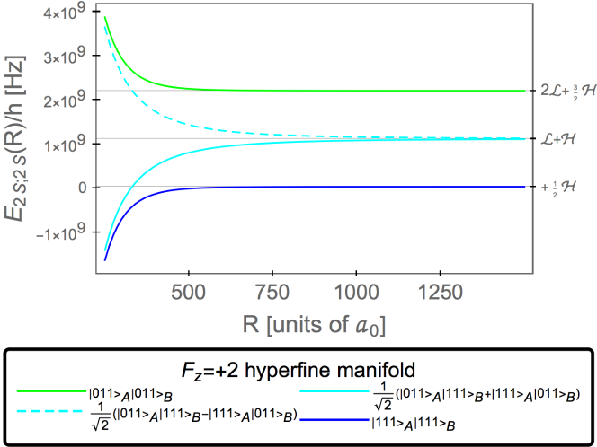
Figure 1: (Color online.) Evolution of the energy levels within the $F_{z}=+2$ hyperfine manifold as a function of interatomic separation. The eigenstates given in the legend are only asymptotic; for finite separation these states mix. One has ${\mathcal{H}}=0.055\,949\,{\mathcal{L}}$ according to Eq. (15). The unit of energy used for the ordinate axis is interaction energy divided by the Planck constant $h$ (left ordinate axis) and given in Hertz (Hz). On the right ordinate axis, we use the Lamb shift ${\mathcal{L}}$ as defined in Eq. (3) as an alternative unit of frequency. The Born–Oppenheimer approximation is used in plotting the interaction energy as a function of the internuclear distance $R$.

III Hamiltonian Matrices in the Hyperfine Subspaces

III.1 Manifold $\maybebm{F_{z}=+2}$

We have already pointed out that the $n=2$, $J=1/2$ Hilbert space naturally separates into subspaces with fixed total hyperfine quantum number $F_{z}=F_{z,a}+F_{z,b}$, according to Eq. (8). We can identify two irreducible subspaces within the $F_{z}=+2$ manifold: the subspace $\mathrm{\@slowromancap i@}$ is composed of the states

$$|\phi_{1}^{\left(\mathrm{\@slowromancap i@}\right)}\rangle =|(0,1,1)_{A}\,(0,1,1)_{B}\rangle\,,$$ (18a)

$$|\phi_{2}^{\left(\mathrm{\@slowromancap i@}\right)}\rangle =|(1,1,1)_{A}\,(1,1,1)_{B}\rangle\,,$$ (18b)

where the Hamiltonian matrix reads

$$H_{F_{z}=+2}^{\left(\mathrm{\@slowromancap i@}\right)}=\left(\begin{array}[]{cc}2{\mathcal{L}}+\tfrac{3}{2}{\mathcal{H}}&-2{\mathcal{V}}\\ -2{\mathcal{V}}&\tfrac{1}{2}{\mathcal{H}}\\ \end{array}\right)\,.$$ (19)

Subspace $\mathrm{\@slowromancap ii@}$ is composed of the states

$$|\phi_{1}^{\left(\mathrm{\@slowromancap ii@}\right)}\rangle= \;|(0,1,1)_{A}\,(1,1,1)_{B}\rangle\,,$$ (20a)

$$|\phi_{2}^{\left(\mathrm{\@slowromancap ii@}\right)}\rangle= \;|(1,1,1)_{A}\,(0,1,1)_{B}\rangle\,,$$ (20b)

where the Hamiltonian matrix reads

$$H_{F_{z}=+2}^{\left(\mathrm{\@slowromancap ii@}\right)}=\left(\begin{array}[]{cccc}{\mathcal{L}}+{\mathcal{H}}&-2{\mathcal{V}}\\ -2{\mathcal{V}}&{\mathcal{L}}+{\mathcal{H}}\\ \end{array}\right)\,.$$ (21)

These subspaces are completely uncoupled. Namely, no state in subspace $\mathrm{\@slowromancap i@}$ is coupled to a state in subspace $\mathrm{\@slowromancap ii@}$.

The eigenvalues of $H_{F_{z}=+2}^{\left(\mathrm{\@slowromancap i@}\right)}$ are given by

$$E_{+}^{\left(\mathrm{\@slowromancap i@}\right)}= \;{\mathcal{H}}+{\mathcal{L}}+\sqrt{4{\mathcal{V}}^{2}+(\tfrac{1}{2}{\mathcal{H}}+{\mathcal{L}})^{2}}$$

$$= \;\tfrac{3}{2}\,{\mathcal{H}}+2{\mathcal{L}}+4\,\frac{{\mathcal{V}}^{2}}{{\mathcal{H}}+2{\mathcal{L}}}+{\mathcal{O}}({\mathcal{V}}^{4})\,,$$ (22a)

$$E_{-}^{\left(\mathrm{\@slowromancap i@}\right)}= \;{\mathcal{H}}+{\mathcal{L}}-\sqrt{4{\mathcal{V}}^{2}+(\tfrac{1}{2}{\mathcal{H}}+{\mathcal{L}})^{2}}$$

$$= \;\tfrac{1}{2}\,{\mathcal{H}}-4\,\frac{{\mathcal{V}}^{2}}{{\mathcal{H}}+2{\mathcal{L}}}+{\mathcal{O}}({\mathcal{V}}^{4})\,,$$ (22b)

with the corresponding eigenvectors

$$|u_{+}^{\left(\mathrm{\@slowromancap i@}\right)}\rangle =\frac{1}{\sqrt{a^{2}+b^{2}}}\left(a\,|\phi_{1}^{\left(\mathrm{\@slowromancap i@}\right)}\rangle+b\,|\phi_{2}^{\left(\mathrm{\@slowromancap i@}\right)}\rangle\right)\,,$$ (23a)

$$|u_{-}^{\left(\mathrm{\@slowromancap i@}\right)}\rangle =\frac{1}{\sqrt{a^{2}+b^{2}}}\left(b\,|\phi_{1}^{\left(\mathrm{\@slowromancap i@}\right)}\rangle-a\,|\phi_{2}^{\left(\mathrm{\@slowromancap i@}\right)}\rangle\right)\,.$$ (23b)

Here the coefficients $a$ and $b$ are given by

$$a =-\frac{2{\mathcal{L}}+{\mathcal{H}}+\sqrt{\left(2{\mathcal{L}}+{\mathcal{H}}\right)^{2}+\left(4{\mathcal{V}}\right)^{2}}}{4{\mathcal{V}}}\,,$$ (24a)

$$b =1\,.$$ (24b)

The eigenenergies of $H_{F_{z}=+2}^{\left(\mathrm{\@slowromancap ii@}\right)}$ are given by

$$E_{\pm}^{\left(\mathrm{\@slowromancap ii@}\right)}={\mathcal{H}}\pm{\mathcal{L}}\pm 2{\mathcal{V}}\,,$$ (25)

with the corresponding eigenvectors,

$$|u_{\pm}^{\left(\mathrm{\@slowromancap ii@}\right)}\rangle=\frac{1}{\sqrt{2}}\,(|\phi_{1}^{\left(\mathrm{\@slowromancap ii@}\right)}\rangle\pm|\phi_{2}^{\left(\mathrm{\@slowromancap ii@}\right)}\rangle)\,.$$ (26)

For ${\mathcal{V}}\to 0$, which corresponds to the large separation limit $R\to+\infty$, these eigenvalues tend toward the (degenerate) diagonal entries of the matrix $H_{F_{z}=+2}^{\left(\mathrm{\@slowromancap ii@}\right)}$.

The eigenstates within the degenerate subspace $\mathrm{\@slowromancap ii@}$ experience a shift of first order in the van der Waals interaction energy ${\mathcal{V}}$, because of the degeneracy of the diagonal entries ${\mathcal{L}}+{\mathcal{H}}$ in Eq. (21); this pattern will be observed for other subspaces in the following. In Fig. 1, we plot the evolution of the eigenvalues (22) and (25) with respect to interatomic separation. The two levels within the subspace $\mathrm{\@slowromancap ii@}$ noticeably experience a far larger interatomic interaction shift from their asymptotic value ${\mathcal{L}}+{\mathcal{H}}$, commensurate with the parametric estimate of the corresponding energy shifts.

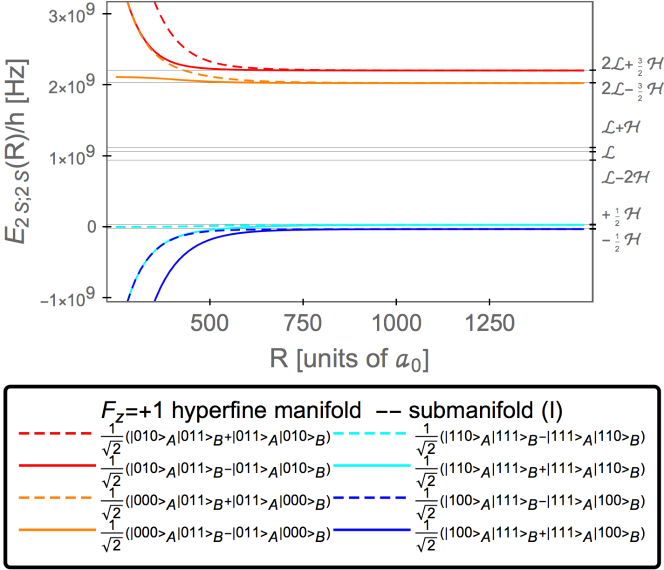
Figure 2: (Color online.) Evolution of the $S$–$S$ and $P$–$P$ energy levels of the submanifold $\mathrm{\@slowromancap i@}$ within the $F_{z}=+1$ hyperfine manifold as a function of interatomic separation. The asymptotic eigenstates given in the legend mix for finite separation. The labeling of the axes is as in Fig. 1.

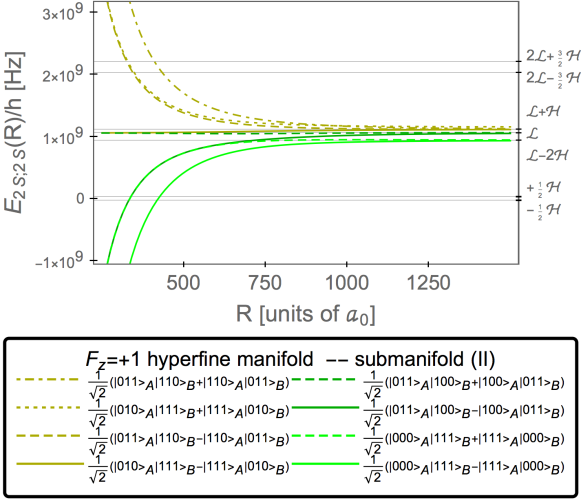
Figure 3: (Color online.) Evolution of the energy levels of the submanifold $\mathrm{\@slowromancap ii@}$ within the $F_{z}=+1$ hyperfine manifold as a function of interatomic separation. The eigenstates given in the legend are only asymptotic. The curve for the seventh state in the legend (counted from the top) has been slightly offset for better readability, in actuality it is virtually indistinguishable from that for the sixth state in the legend.

III.2 Manifold $\maybebm{F_{z}=+1}$

We can identify two irreducible subspaces within the $F_{z}=+1$ manifold. Subspace $\mathrm{\@slowromancap i@}$ is composed of the following states, with both atoms either being in $S$, or both in $P$ states,

$$|\psi_{1}^{\left(\mathrm{\@slowromancap i@}\right)}\rangle= \;|(0,0,0)_{A}\,(0,1,1)_{B}\rangle\,,\qquad|\psi_{2}^{\left(\mathrm{\@slowromancap i@}\right)}\rangle=|(0,1,0)_{A}\,(0,1,1)_{B}\rangle\,,\qquad|\psi_{3}^{\left(\mathrm{\@slowromancap i@}\right)}\rangle=|(0,1,1)_{A}\,(0,0,0)_{B}\rangle\,,$$ (27)

$$|\psi_{4}^{\left(\mathrm{\@slowromancap i@}\right)}\rangle= \;|(0,1,1)_{A}\,(0,1,0)_{B}\rangle\,,\qquad|\psi_{5}^{\left(\mathrm{\@slowromancap i@}\right)}\rangle=|(1,0,0)_{A}\,(1,1,1)_{B}\rangle\,,\qquad|\psi_{6}^{\left(\mathrm{\@slowromancap i@}\right)}\rangle=|(1,1,0)_{A}\,(1,1,1)_{B}\rangle\,,$$

$$|\psi_{7}^{\left(\mathrm{\@slowromancap i@}\right)}\rangle= \;|(1,1,1)_{A}\,(1,0,0)_{B}\rangle\,,\qquad|\psi_{8}^{\left(\mathrm{\@slowromancap i@}\right)}\rangle=|(1,1,1)_{A}\,(1,1,0)_{B}\rangle\,,$$

and the Hamiltonian matrix reads

$$H_{F_{z}=+1}^{\left(\mathrm{\@slowromancap i@}\right)}= \;\left(\begin{array}[]{cccccccc}2{\mathcal{L}}-\tfrac{3}{2}{\mathcal{H}}&0&0&0&0&-2{\mathcal{V}}&{\mathcal{V}}&-{\mathcal{V}}\\ 0&2{\mathcal{L}}+\tfrac{3}{2}{\mathcal{H}}&0&0&-2{\mathcal{V}}&0&-{\mathcal{V}}&{\mathcal{V}}\\ 0&0&2{\mathcal{L}}-\tfrac{3}{2}{\mathcal{H}}&0&{\mathcal{V}}&-{\mathcal{V}}&0&-2{\mathcal{V}}\\ 0&0&0&2{\mathcal{L}}+\tfrac{3}{2}{\mathcal{H}}&-{\mathcal{V}}&{\mathcal{V}}&-2{\mathcal{V}}&0\\ 0&-2{\mathcal{V}}&{\mathcal{V}}&-{\mathcal{V}}&-\tfrac{1}{2}{\mathcal{H}}&0&0&0\\ -2{\mathcal{V}}&0&-{\mathcal{V}}&{\mathcal{V}}&0&\tfrac{1}{2}{\mathcal{H}}&0&0\\ {\mathcal{V}}&-{\mathcal{V}}&0&-2{\mathcal{V}}&0&0&-\tfrac{1}{2}{\mathcal{H}}&0\\ -{\mathcal{V}}&\mathcal{V}&-2{\mathcal{V}}&0&0&0&0&\tfrac{1}{2}{\mathcal{H}}\end{array}\right)\,.$$ (36)

Subspace $\mathrm{\@slowromancap ii@}$ is composed of the following states, where one atom is in a $S$, and the other, in a $P$ state,

$$|\psi_{1}^{\left(\mathrm{\@slowromancap ii@}\right)}\rangle= \;|(0,0,0)_{A}\,(1,1,1)_{B}\rangle\,,\qquad|\psi_{2}^{\left(\mathrm{\@slowromancap ii@}\right)}\rangle=|(0,1,0)_{A}\,(1,1,1)_{B}\rangle\,,\qquad|\psi_{3}^{\left(\mathrm{\@slowromancap ii@}\right)}\rangle=|(0,1,1)_{A}\,(1,0,0)_{B}\rangle\,,$$ (37)

$$|\psi_{4}^{\left(\mathrm{\@slowromancap ii@}\right)}\rangle= \;|(0,1,1)_{A}\,(1,1,0)_{B}\rangle\,,\qquad|\psi_{5}^{\left(\mathrm{\@slowromancap ii@}\right)}\rangle=|(1,0,0)_{A}\,(0,1,1)_{B}\rangle\,,\qquad|\psi_{6}^{\left(\mathrm{\@slowromancap ii@}\right)}\rangle=|(1,1,0)_{A}\,(0,1,1)_{B}\rangle\,,$$

$$|\psi_{7}^{\left(\mathrm{\@slowromancap ii@}\right)}\rangle= \;|(1,1,1)_{A}\,(0,0,0)_{B}\rangle\,,\qquad|\psi_{8}^{\left(\mathrm{\@slowromancap ii@}\right)}\rangle=|(1,1,1)_{A}\,(0,1,0)_{B}\rangle\,,$$

and the Hamiltonian matrix reads

$$H_{F_{z}=+1}^{\left(\mathrm{\@slowromancap ii@}\right)}= \;\left(\begin{array}[]{cccccccc}{\mathcal{L}}-2{\mathcal{H}}&0&0&0&0&-2{\mathcal{V}}&{\mathcal{V}}&-{\mathcal{V}}\\ 0&{\mathcal{L}}+{\mathcal{H}}&0&0&-2{\mathcal{V}}&0&-{\mathcal{V}}&{\mathcal{V}}\\ 0&0&{\mathcal{L}}&0&{\mathcal{V}}&-{\mathcal{V}}&0&-2{\mathcal{V}}\\ 0&0&0&{\mathcal{L}}+{\mathcal{H}}&-{\mathcal{V}}&{\mathcal{V}}&-2{\mathcal{V}}&0\\ 0&-2{\mathcal{V}}&{\mathcal{V}}&-{\mathcal{V}}&{\mathcal{L}}&0&0&0\\ -2{\mathcal{V}}&0&-{\mathcal{V}}&{\mathcal{V}}&0&{\mathcal{L}}+{\mathcal{H}}&0&0\\ {\mathcal{V}}&-{\mathcal{V}}&0&-2{\mathcal{V}}&0&0&{\mathcal{L}}-2{\mathcal{H}}&0\\ -{\mathcal{V}}&\mathcal{V}&-2{\mathcal{V}}&0&0&0&0&{\mathcal{L}}+{\mathcal{H}}\end{array}\right)\,.$$ (46)

These two submanifolds are, again, completely uncoupled, as a consequence of the selection rules between $S$ and $P$ states. One observes that within the subspace $\mathrm{\@slowromancap i@}$, no two degenerate levels are coupled to each other, resulting in second-order van der Waals energy shifts. On the other hand, the following subspaces, within the subspace $\mathrm{\@slowromancap ii@}$, can be identified as being degenerate with respect to the unperturbed Hamiltonian, and having states coupled by nonvanishing off-diagonal elements. We first have a subspace spanned by

$$|\psi^{\left(A\right)}_{1}\rangle=|\psi^{\left(\mathrm{\@slowromancap ii@}\right)}_{1}\rangle\,,\qquad|\psi^{\left(A\right)}_{2}\rangle=|\psi^{\left(\mathrm{\@slowromancap ii@}\right)}_{7}\rangle\,.$$ (47)

These states are composed of a singlet $S$ and a triplet $P$ state, and hence the diagonal entries in the Hamiltonian matrix are $(-\tfrac{9}{4}{\mathcal{H}}+{\mathcal{L}})+(\tfrac{1}{4}{\mathcal{H}})=-2{\mathcal{H}}+{\mathcal{L}}$. The Hamiltonian matrix is

$$H_{F_{z}=+1}^{(A)}=\left(\begin{array}[]{cc}{\mathcal{L}}-2{\mathcal{H}}&{\mathcal{V}}\\ {\mathcal{V}}&{\mathcal{L}}-2{\mathcal{H}}\\ \end{array}\right).$$ (48)

The eigenvalues are

$$E^{(A)}_{\pm}={\mathcal{L}}-2{\mathcal{H}}\pm{\mathcal{V}}\,,$$ (49)

with the corresponding eigenvectors,

$$|u_{\pm}^{(A)}\rangle=\frac{1}{\sqrt{2}}\,\left(|\psi^{(A)}_{1}\rangle\pm|\psi^{(A)}_{2}\rangle\right)\,.$$ (50)

Note that the designation of a degenerate subspace, for the $F_{z}=+1$ subspace, does not imply that there are no couplings to any other states within the manifold; however, the couplings relating the degenerate states will become dominant for close approach.

A second degenerate subspace is given as

$$|\psi^{(B)}_{1}\rangle=|\psi^{\left(\mathrm{\@slowromancap ii@}\right)}_{3}\rangle\,,\qquad|\psi^{(B)}_{2}\rangle=|\psi^{\left(\mathrm{\@slowromancap ii@}\right)}_{5}\rangle\,.$$ (51)

These states are composed of a triplet $S$ and a singlet $P$ state, and hence the diagonal entries in the Hamiltonian matrix are $(\tfrac{3}{4}{\mathcal{H}}+{\mathcal{L}})-(\tfrac{3}{4}{\mathcal{H}})={\mathcal{L}}$. The Hamiltonian matrix is

$$H_{F_{z}=+1}^{(B)}=\left(\begin{array}[]{cc}{\mathcal{L}}&{\mathcal{V}}\\ {\mathcal{V}}&{\mathcal{L}}\\ \end{array}\right).$$ (52)

The eigenvalues are

$$E^{(B)}_{\pm}={\mathcal{L}}\pm{\mathcal{V}}\,,$$ (53)

with the corresponding eigenvectors,

$$|u_{\pm}^{(B)}\rangle=\frac{1}{\sqrt{2}}\,\left(|\psi^{(B)}_{1}\rangle\pm|\psi^{(B)}_{2}\right).$$ (54)

The most complicated degenerate subspace is given by the vectors

$$|\psi^{(C)}_{1}\rangle= \;|\psi^{\left(\mathrm{\@slowromancap ii@}\right)}_{2}\rangle\,,\qquad|\psi^{(C)}_{2}\rangle=|\psi^{\left(\mathrm{\@slowromancap ii@}\right)}_{4}\rangle\,,$$ (55)

$$|\psi^{(C)}_{3}\rangle= \;|\psi^{\left(\mathrm{\@slowromancap ii@}\right)}_{6}\rangle\,,\qquad|\psi^{(C)}_{4}\rangle=|\psi^{\left(\mathrm{\@slowromancap ii@}\right)}_{8}\rangle\,.$$ (56)

The Hamiltonian matrix is

$$H_{F_{z}=+1}^{(C)}=\left(\begin{array}[]{cccc}{\mathcal{L}}+{\mathcal{H}}&0&0&{\mathcal{V}}\\ 0&{\mathcal{L}}+{\mathcal{H}}&{\mathcal{V}}&0\\ 0&{\mathcal{V}}&{\mathcal{L}}+{\mathcal{H}}&0\\ {\mathcal{V}}&0&0&{\mathcal{L}}+{\mathcal{H}}\\ \end{array}\right)\,,$$ (57)

which again decouples into two $2\times 2$ matrices, just like we saw in the case of $H_{F_{z}=+2}$. The eigenvalues are

$$E^{(C)}_{\pm}={\mathcal{H}}+{\mathcal{L}}\pm{\mathcal{V}}\,,$$ (58)

where the eigenvectors for $|u_{\pm,i}^{(C)}\rangle$ (with $i=1,2$ because of the degeneracy of the eigenvalues) are given by

$$|u_{\pm,1}^{(C)}\rangle =\frac{1}{\sqrt{2}}\,\left(|\psi^{(C)}_{1}\rangle\pm|\psi^{(C)}_{4}\right)\rangle\,,$$ (59a)

$$|u_{\pm,2}^{(C)}\rangle =\frac{1}{\sqrt{2}}\,\left(|\psi^{(C)}_{2}\rangle\pm|\psi^{(C)}_{3}\right)\rangle\,.$$ (59b)

In Figs. 2 and 3, we plot the evolution of the eigenvalues of the matrices (36) and (46) with respect to interatomic separation. The larger energy shifts within the subspace $\mathrm{\@slowromancap ii@}$ are noticeable. A feature exhibited by the $F_{z}=+1$ manifold which was not present in the $F_{z}=+2$ manifold is that of level crossings: for sufficiently small interatomic separation ($R<500\,a_{0}$), the eigenenergies of some of the states from the submanifolds $\mathrm{\@slowromancap i@}$ and $\mathrm{\@slowromancap ii@}$ in fact cross (these crossings would be visible if one were to superimpose Figs. 2 and 3), while there are no level crossings between states belonging to the same submanifold.

Figure 4: (Color online.) Evolution of the energy levels of the submanifold $\mathrm{\@slowromancap i@}$ within the $F_{z}=0$ hyperfine manifold as a function of interatomic separation. Energetically, the $S$–$S$ states are above the $P$–$P$ states. The eigenstates given in the legend are only asymptotic; for finite separation these states mix. Some of the curves [namely, the third (from the top), sixth and twelfth] have been slightly offset for better readability. Notice that, for sufficiently close separation ($R<1\,000\,a_{0}$), we witness some level crossings between levels within the same submanifold $\mathrm{\@slowromancap i@}$. The coefficients $\alpha_{\pm}$ and $\beta_{\pm}$ are determined by second-order perturbation theory and given by Eq. (123).

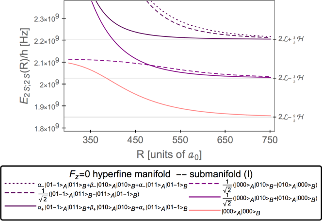
Figure 5: (Color online.) Evolution of the energy levels of the $2S$–$2S$ states within the $F_{z}=0$ hyperfine manifold (subspace $\mathrm{\@slowromancap i@}$) as a function of the interatomic separation (close-up of the “upper” levels in Fig. 4). The eigenstates given in the legend are only asymptotic; for finite separation these states mix. No offsets are used here. Notice that we witness one level crossing. The coefficients $\alpha_{\pm}$ and $\beta_{\pm}$ are determined by second-order perturbation theory and given by Eq. (123).

III.3 Manifold $\maybebm{F_{z}=0}$

We can identify two irreducible subspaces within the $F_{z}=0$ manifold: the subspace $\mathrm{\@slowromancap i@}$ is composed of states with both atoms in $S$, or both atoms in $P$ levels,

$$|\Psi_{1}^{\left(\mathrm{\@slowromancap i@}\right)}\rangle= \;|(0,0,0)_{A}\,(0,0,0)_{B}\rangle\,,\qquad|\Psi_{2}^{\left(\mathrm{\@slowromancap i@}\right)}\rangle=|(0,0,0)_{A}\,(0,1,0)_{B}\rangle\,,\qquad|\Psi_{3}^{\left(\mathrm{\@slowromancap i@}\right)}\rangle=|(0,1,-1)_{A}\,(0,1,1)_{B}\rangle\,,$$ (60)

$$|\Psi_{4}^{\left(\mathrm{\@slowromancap i@}\right)}\rangle= \;|(0,1,0)_{A}\,(0,0,0)_{B}\rangle\,,\qquad|\Psi_{5}^{\left(\mathrm{\@slowromancap i@}\right)}\rangle=|(0,1,0)_{A}\,(0,1,0)_{B}\rangle\,,\qquad|\Psi_{6}^{\left(\mathrm{\@slowromancap i@}\right)}\rangle=|(0,1,1)_{A}\,(0,1,-1)_{B}\rangle\,,$$

$$|\Psi_{7}^{\left(\mathrm{\@slowromancap i@}\right)}\rangle= \;|(1,0,0)_{A}\,(1,0,0)_{B}\rangle\,,\qquad|\Psi_{8}^{\left(\mathrm{\@slowromancap i@}\right)}\rangle=|(1,0,0)_{A}\,(1,1,0)_{B}\rangle\,,\qquad|\Psi_{9}^{\left(\mathrm{\@slowromancap i@}\right)}\rangle=|(1,1,-1)_{A}\,(1,1,1)_{B}\rangle\,,$$

$$|\Psi_{10}^{\left(\mathrm{\@slowromancap i@}\right)}\rangle= \;|(1,1,0)_{A}\,(1,0,0)_{B}\rangle\,,\qquad|\Psi_{11}^{\left(\mathrm{\@slowromancap i@}\right)}\rangle=|(1,1,0)_{A}\,(1,1,0)_{B}\rangle\,,\qquad|\Psi_{12}^{\left(\mathrm{\@slowromancap i@}\right)}\rangle=|(1,1,1)_{A}\,(1,1,-1)_{B}\rangle\,$$

and the Hamiltonian matrix reads

$$H_{F_{z}=0}^{\left(\mathrm{\@slowromancap i@}\right)}= \;\left(\begin{array}[]{cccccccccccc}2{\mathcal{L}}-\tfrac{9}{2}{\mathcal{H}}&0&0&0&0&0&0&0&-{\mathcal{V}}&0&-2{\mathcal{V}}&-{\mathcal{V}}\\ 0&2{\mathcal{L}}-\tfrac{3}{2}{\mathcal{H}}&0&0&0&0&0&0&{\mathcal{V}}&-2{\mathcal{V}}&0&-{\mathcal{V}}\\ 0&0&2{\mathcal{L}}+\tfrac{3}{2}{\mathcal{H}}&0&0&0&-{\mathcal{V}}&{\mathcal{V}}&2{\mathcal{V}}&-{\mathcal{V}}&{\mathcal{V}}&0\\ 0&0&0&2{\mathcal{L}}-\tfrac{3}{2}{\mathcal{H}}&0&0&0&-2{\mathcal{V}}&-{\mathcal{V}}&0&0&{\mathcal{V}}\\ 0&0&0&0&2{\mathcal{L}}+\tfrac{3}{2}{\mathcal{H}}&0&-2{\mathcal{V}}&0&{\mathcal{V}}&0&0&{\mathcal{V}}\\ 0&0&0&0&0&2{\mathcal{L}}+\tfrac{3}{2}{\mathcal{H}}&-{\mathcal{V}}&-{\mathcal{V}}&0&{\mathcal{V}}&{\mathcal{V}}&2{\mathcal{V}}\\ 0&0&-{\mathcal{V}}&0&-2{\mathcal{V}}&-{\mathcal{V}}&-\tfrac{3}{2}{\mathcal{H}}&0&0&0&0&0\\ 0&0&{\mathcal{V}}&-2{\mathcal{V}}&0&-{\mathcal{V}}&0&-\tfrac{1}{2}{\mathcal{H}}&0&0&0&0\\ -{\mathcal{V}}&{\mathcal{V}}&2{\mathcal{V}}&-{\mathcal{V}}&{\mathcal{V}}&0&0&0&\tfrac{1}{2}{\mathcal{H}}&0&0&0\\ 0&-2{\mathcal{V}}&-{\mathcal{V}}&0&0&{\mathcal{V}}&0&0&0&-\tfrac{1}{2}{\mathcal{H}}&0&0\\ -2{\mathcal{V}}&0&{\mathcal{V}}&0&0&{\mathcal{V}}&0&0&0&0&\tfrac{1}{2}{\mathcal{H}}&0\\ -{\mathcal{V}}&-{\mathcal{V}}&0&{\mathcal{V}}&{\mathcal{V}}&2{\mathcal{V}}&0&0&0&0&0&\tfrac{1}{2}{\mathcal{H}}\end{array}\right)\,.$$ (73)

Subspace $\mathrm{\@slowromancap ii@}$ is composed of the $S$–$P$ and $P$–$S$ combinations,

$$|\Psi_{1}^{\left(\mathrm{\@slowromancap ii@}\right)}\rangle= |(0,0,0)_{A}\,(1,0,0)_{B}\rangle\,,\qquad|\Psi_{2}^{\left(\mathrm{\@slowromancap ii@}\right)}\rangle=\;|(0,0,0)_{A}\,(1,1,0)_{B}\rangle\,,\qquad|\Psi_{3}^{\left(\mathrm{\@slowromancap ii@}\right)}\rangle=|(0,1,-1)_{A}\,(1,1,1)_{B}\rangle\,,$$ (74)

$$|\Psi_{4}^{\left(\mathrm{\@slowromancap ii@}\right)}\rangle= |(0,1,0)_{A}\,(1,0,0)_{B}\rangle\,,\qquad|\Psi_{5}^{\left(\mathrm{\@slowromancap ii@}\right)}\rangle=\;|(0,1,0)_{A}\,(1,1,0)_{B}\rangle\,,\qquad|\Psi_{6}^{\left(\mathrm{\@slowromancap ii@}\right)}\rangle=|(0,1,1)_{A}\,(1,1,-1)_{B}\rangle\,,$$

$$|\Psi_{7}^{\left(\mathrm{\@slowromancap ii@}\right)}\rangle= \;|(1,0,0)_{A}\,(0,0,0)_{B}\rangle\,,\qquad|\Psi_{8}^{\left(\mathrm{\@slowromancap ii@}\right)}\rangle=|(1,0,0)_{A}\,(0,1,0)_{B}\rangle\,,\qquad|\Psi_{9}^{\left(\mathrm{\@slowromancap ii@}\right)}\rangle=|(1,1,-1)_{A}\,(0,1,1)_{B}\rangle\,,$$

$$|\Psi_{10}^{\left(\mathrm{\@slowromancap ii@}\right)}\rangle= \;|(1,1,0)_{A}\,(0,0,0)_{B}\rangle\,,\qquad|\Psi_{11}^{\left(\mathrm{\@slowromancap ii@}\right)}\rangle=|(1,1,0)_{A}\,(0,1,0)_{B}\rangle\,,\qquad|\Psi_{12}^{\left(\mathrm{\@slowromancap ii@}\right)}\rangle=|(1,1,1)_{A}\,(0,1,-1)_{B}\rangle\,,$$

and the Hamiltonian matrix reads

$$H_{F_{z}=0}^{\left(\mathrm{\@slowromancap ii@}\right)}= \;\left(\begin{array}[]{cccccccccccc}{\mathcal{L}}-3{\mathcal{H}}&0&0&0&0&0&0&0&-{\mathcal{V}}&0&-2{\mathcal{V}}&-{\mathcal{V}}\\ 0&{\mathcal{L}}-2{\mathcal{H}}&0&0&0&0&0&0&{\mathcal{V}}&-2{\mathcal{V}}&0&-{\mathcal{V}}\\ 0&0&{\mathcal{L}}+{\mathcal{H}}&0&0&0&-{\mathcal{V}}&{\mathcal{V}}&2{\mathcal{V}}&-{\mathcal{V}}&{\mathcal{V}}&0\\ 0&0&0&{\mathcal{L}}&0&0&0&-2{\mathcal{V}}&-{\mathcal{V}}&0&0&{\mathcal{V}}\\ 0&0&0&0&{\mathcal{L}}+{\mathcal{H}}&0&-2{\mathcal{V}}&0&{\mathcal{V}}&0&0&{\mathcal{V}}\\ 0&0&0&0&0&{\mathcal{L}}+{\mathcal{H}}&-{\mathcal{V}}&-{\mathcal{V}}&0&{\mathcal{V}}&{\mathcal{V}}&2{\mathcal{V}}\\ 0&0&-{\mathcal{V}}&0&-2{\mathcal{V}}&-{\mathcal{V}}&{\mathcal{L}}-3{\mathcal{H}}&0&0&0&0&0\\ 0&0&{\mathcal{V}}&-2{\mathcal{V}}&0&-{\mathcal{V}}&0&{\mathcal{L}}&0&0&0&0\\ -{\mathcal{V}}&{\mathcal{V}}&2{\mathcal{V}}&-{\mathcal{V}}&{\mathcal{V}}&0&0&0&{\mathcal{L}}+{\mathcal{H}}&0&0&0\\ 0&-2{\mathcal{V}}&-{\mathcal{V}}&0&0&{\mathcal{V}}&0&0&0&{\mathcal{L}}-2{\mathcal{H}}&0&0\\ -2{\mathcal{V}}&0&{\mathcal{V}}&0&0&{\mathcal{V}}&0&0&0&0&{\mathcal{L}}+{\mathcal{H}}&0\\ -{\mathcal{V}}&-{\mathcal{V}}&0&{\mathcal{V}}&{\mathcal{V}}&2{\mathcal{V}}&0&0&0&0&0&{\mathcal{L}}+{\mathcal{H}}\end{array}\right)\,.$$ (87)

Again, we notice that within the subspace $\mathrm{\@slowromancap i@}$, no two degenerate levels are coupled to each other. On the other hand, the following subspaces, within the subspace $\mathrm{\@slowromancap ii@}$, can be identified as being degenerate with respect to the unperturbed Hamiltonian, and having states coupled by nonvanishing off-diagonal elements.

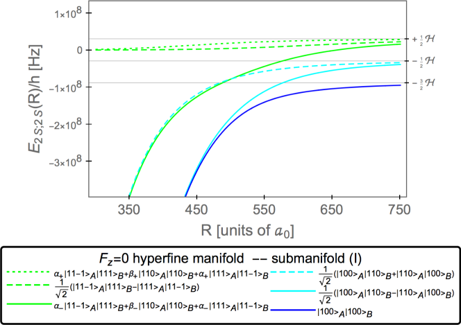
Figure 6: (Color online.) Evolution of the energy levels of the $2P$–$2P$ states within the $F_{z}=0$ hyperfine manifold (subspace $\mathrm{\@slowromancap i@}$) as a function of interatomic separation (close-up of the “lower” levels in Fig. 4). Asymptotic eigenstates used in the legend mix for finite separation. No offsets are used here. Notice that we witness one level crossing. The coefficients $\alpha_{\pm}$ and $\beta_{\pm}$ are determined by second-order perturbation theory and given by Eq. (123).

The first degenerate subspace is given as follows,

$$|\Psi^{(A)}_{1}\rangle=|\Psi^{\left(\mathrm{\@slowromancap ii@}\right)}_{2}\rangle\,,\qquad|\Psi^{(A)}_{2}\rangle=|\Psi^{\left(\mathrm{\@slowromancap ii@}\right)}_{10}\rangle\,.$$ (88)

The Hamiltonian matrix reads as

$$H_{F_{z}=0}^{(A)}=\left(\begin{array}[]{cccc}{\mathcal{L}}-2{\mathcal{H}}&-2{\mathcal{V}}\\ -2{\mathcal{V}}&{\mathcal{L}}-2{\mathcal{H}}\\ \end{array}\right)\,.$$ (89)

The eigensystem is given by

$$E^{(A)}_{\pm}={\mathcal{L}}-2{\mathcal{H}}\pm 2{\mathcal{V}}\,,\quad|u_{\pm}^{(A)}\rangle=\frac{1}{\sqrt{2}}\,(|\Psi_{1}^{(A)}\rangle\mp\Psi_{2}^{(A)}\rangle)\,.$$ (90)

The second degenerate subspace is

$$|\Psi^{(B)}_{1}\rangle=|\Psi^{\left(\mathrm{\@slowromancap ii@}\right)}_{4}\rangle\,,\qquad|\Psi^{(B)}_{2}\rangle=|\Psi^{\left(\mathrm{\@slowromancap ii@}\right)}_{8}\rangle\,,$$ (91)

with the Hamiltonian matrix

$$H_{F_{z}=0}^{(B)}=\left(\begin{array}[]{cc}{\mathcal{L}}&-2{\mathcal{V}}\\ -2{\mathcal{V}}&{\mathcal{L}}\\ \end{array}\right)$$ (92)

and the eigensystem

$$E^{(B)}_{\pm}={\mathcal{L}}\pm 2{\mathcal{V}}\,,\quad\qquad|u_{\pm}^{(B)}\rangle=\frac{1}{\sqrt{2}}\,(|\Psi_{1}^{(B)}\rangle\mp\Psi_{2}^{(B)}\rangle)\,.$$ (93)

The third degenerate subspace is more complicated, and is spanned by the six state vectors

$$|\Psi^{(C)}_{1}\rangle= \;|\Psi^{\left(\mathrm{\@slowromancap ii@}\right)}_{3}\rangle\,,\qquad|\Psi^{(C)}_{2}\rangle=|\Psi^{\left(\mathrm{\@slowromancap ii@}\right)}_{5}\rangle\,,$$ (94a)

$$|\Psi^{(C)}_{3}\rangle= \;|\Psi^{\left(\mathrm{\@slowromancap ii@}\right)}_{6}\rangle\,,\qquad|\Psi^{(C)}_{4}\rangle=|\Psi^{\left(\mathrm{\@slowromancap ii@}\right)}_{9}\rangle\,,$$ (94b)

$$|\Psi^{(C)}_{5}\rangle= \;|\Psi^{\left(\mathrm{\@slowromancap ii@}\right)}_{11}\rangle\,,\qquad|\Psi^{(C)}_{6}\rangle=|\Psi^{\left(\mathrm{\@slowromancap ii@}\right)}_{12}\rangle\,.$$ (94c)

The six-dimensional submatrix is

$$H_{F_{z}=0}^{(C)}=\left(\begin{array}[]{cccccc}{\mathcal{L}}+{\mathcal{H}}&0&0&2{\mathcal{V}}&{\mathcal{V}}&0\\ 0&{\mathcal{L}}+{\mathcal{H}}&0&{\mathcal{V}}&0&{\mathcal{V}}\\ 0&0&{\mathcal{L}}+{\mathcal{H}}&0&{\mathcal{V}}&2{\mathcal{V}}\\ 2{\mathcal{V}}&{\mathcal{V}}&0&{\mathcal{L}}+{\mathcal{H}}&0&0\\ {\mathcal{V}}&0&{\mathcal{V}}&0&{\mathcal{L}}+{\mathcal{H}}&0\\ 0&{\mathcal{V}}&2{\mathcal{V}}&0&0&{\mathcal{L}}+{\mathcal{H}}\\ \end{array}\right)\,.$$ (95)

The eigenvalues are

$$E^{(C)}_{\pm,1}= \;{\mathcal{H}}+{\mathcal{L}}\pm 2\,{\mathcal{V}}\,,$$ (96a)

$$E^{(C)}_{\pm,2}= \;{\mathcal{H}}+{\mathcal{L}}\pm(\sqrt{3}+1)\,{\mathcal{V}}\,,$$ (96b)

$$E^{(C)}_{\pm,3}= \;{\mathcal{H}}+{\mathcal{L}}\pm(\sqrt{3}-1)\,{\mathcal{V}}\,,$$ (96c)

and the eigenvectors are

$$u^{(C)}_{+,1}= \;\frac{1}{2}\,\left(|\Psi^{(C)}_{1}\rangle-|\Psi^{(C)}_{3}\rangle+|\Psi^{(C)}_{4}\rangle-|\Psi^{(C)}_{6}\rangle\right)\,,$$ (97a)

$$u^{(C)}_{-,1}= \;\frac{1}{2}\,\left(|\Psi^{(C)}_{1}\rangle-|\Psi^{(C)}_{3}\rangle-|\Psi^{(C)}_{4}\rangle+|\Psi^{(C)}_{6}\rangle\right)\,,$$ (97b)

$$u^{(C)}_{+,2}= \;\frac{1}{2\sqrt{3-\sqrt{3}}}\,\left(|\Psi^{(C)}_{1}\rangle+(\sqrt{3}-1)\,|\Psi^{(C)}_{2}\rangle+|\Psi^{(C)}_{3}\rangle+|\Psi^{(C)}_{4}\rangle+(\sqrt{3}-1)\,|\Psi^{(C)}_{5}\rangle+|\Psi^{(C)}_{6}\rangle\right)\,,$$ (97c)

$$u^{(C)}_{-,2}= \;\frac{1}{2\sqrt{3-\sqrt{3}}}\,\left(|\Psi^{(C)}_{1}\rangle+(\sqrt{3}-1)\,|\Psi^{(C)}_{2}\rangle+|\Psi^{(C)}_{3}\rangle-|\Psi^{(C)}_{4}\rangle-(\sqrt{3}-1)\,|\Psi^{(C)}_{5}\rangle-|\Psi^{(C)}_{6}\rangle\right)\,,$$ (97d)

$$u^{(C)}_{+,3}= \;\frac{1}{2\sqrt{3+\sqrt{3}}}\,\left(|\Psi^{(C)}_{1}\rangle-(\sqrt{3}+1)\,|\Psi^{(C)}_{2}\rangle+|\Psi^{(C)}_{3}\rangle-|\Psi^{(C)}_{4}\rangle+(\sqrt{3}+1)\,|\Psi^{(C)}_{5}\rangle-|\Psi^{(C)}_{6}\rangle\right)\,,$$ (97e)

$$u^{(C)}_{-,3}= \;\frac{1}{2\sqrt{3+\sqrt{3}}}\,\left(|\Psi^{(C)}_{1}\rangle-(\sqrt{3}+1)\,|\Psi^{(C)}_{2}\rangle+|\Psi^{(C)}_{3}\rangle+|\Psi^{(C)}_{4}\rangle-(\sqrt{3}+1)\,|\Psi^{(C)}_{5}\rangle+|\Psi^{(C)}_{6}\rangle\right)\,.$$ (97f)

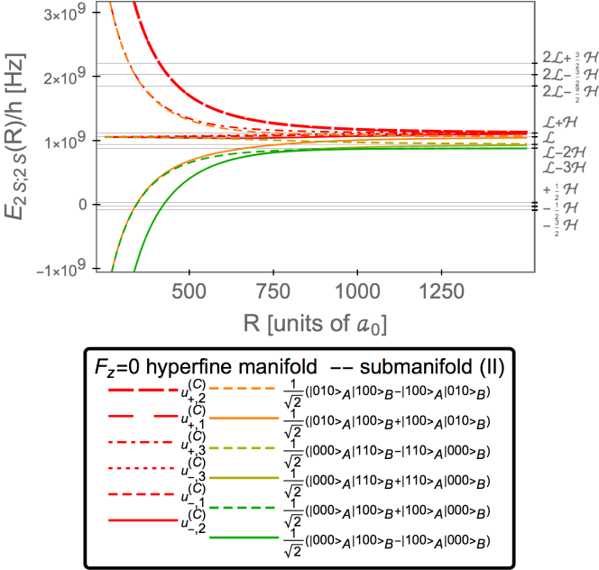
Figure 7: (Color online.) Evolution of the $S$–$P$ and $P$–$S$ energy levels within the $F_{z}=0$ hyperfine manifold (submanifold $\mathrm{\@slowromancap ii@}$) as a function of interatomic separation. The eigenstates given in the legend are only asymptotic, for finite separation these states mix. Some of the curves (namely, for the ninth and twelfth states in the legend, counted from the top) have been slightly offset for better readability. Notice that, for sufficiently close separation ($R<1\,000\,a_{0}$), we witness some level crossings between levels within the same submanifold $\mathrm{\@slowromancap ii@}$. The first six states are given in Eq. (97).

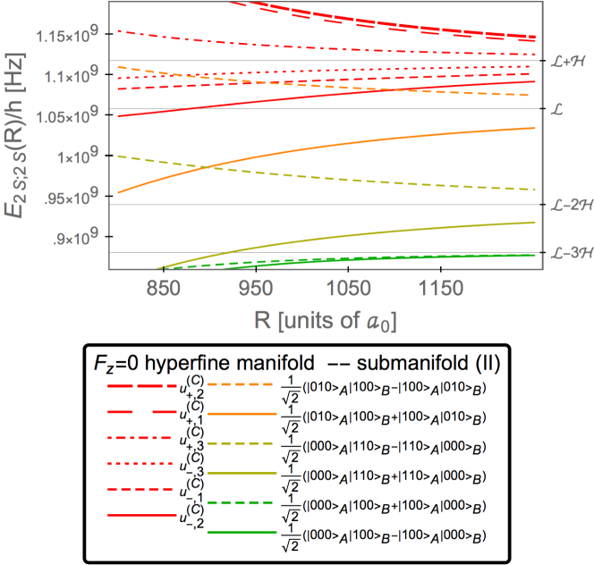
Figure 8: (Color online.) Close-up of the evolution of the energy levels of the $2S$–$2P$ and $2P$–$2S$ states (submanifold $\mathrm{\@slowromancap ii@}$) within the $F_{z}=0$ hyperfine manifold as a function of interatomic separation. For the legend, we use the asymptotic eigenstates for large separation. No offsets are used here. Notice that we witness four level crossings. The first six states are given by Eq. (97).

In Figs. 4—8, we plot the evolution of the eigenvalues of matrices (73) and (87) with respect to interatomic separation. Notice again that the twelve levels within the subspace $\mathrm{\@slowromancap ii@}$ noticeably leave their asymptotic values (of order $\sim{\mathcal{L}}$) for far larger separations than the twelve levels within the subspace $\mathrm{\@slowromancap i@}$, as predicted above by analyzing the order of the corresponding energy shifts. A feature exhibited by the $F_{z}=0$ manifold which was not present in the $F_{z}=+1$ manifold is that of level crossings between levels within the same irreducible submanifold: for sufficiently small interatomic separations ($R<1\,000\,a_{0}$), the eigenenergies of some of the states from the submanifold $\mathrm{\@slowromancap i@}$ cross between themselves, and so do some in manifold $\mathrm{\@slowromancap ii@}$. For better visibility of these intra-manifold crossings, we present them in Figs. 5 and 6, as well as in Fig. 8. For even smaller interatomic separations ($R<500\,a_{0}$) we obtain, again, crossings between levels in manifolds $\mathrm{\@slowromancap i@}$ and $\mathrm{\@slowromancap ii@}$.

As shown in Fig. 4, some levels within submanifold $\mathrm{\@slowromancap i@}$, namely, on the one hand, the levels

$$|\Psi_{3}^{\left(\mathrm{\@slowromancap i@}\right)}\rangle= \;|(0,1,-1)_{A}\,(0,1,1)_{B}\rangle\,,$$ (98a)

$$|\Psi_{5}^{\left(\mathrm{\@slowromancap i@}\right)}\rangle= \;|(0,1,0)_{A}\,(0,1,0)_{B}\rangle\,,$$ (98b)

$$|\Psi_{6}^{\left(\mathrm{\@slowromancap i@}\right)}\rangle= \;|(0,1,1)_{A}\,(0,1,-1)_{B}\rangle\,,$$ (98c)

that have asymptotic energy $2{\mathcal{L}}+\tfrac{3}{2}{\mathcal{H}}$; and, on the other hand,

$$|\Psi_{9}^{\left(\mathrm{\@slowromancap i@}\right)}\rangle= \;|(1,1,-1)_{A}\,(1,1,1)_{B}\rangle\,,$$ (99a)

$$|\Psi_{11}^{\left(\mathrm{\@slowromancap i@}\right)}\rangle= \;|(1,1,0)_{A}\,(1,1,0)_{B}\rangle\,,$$ (99b)

$$|\Psi_{12}^{\left(\mathrm{\@slowromancap i@}\right)}\rangle= \;|(1,1,1)_{A}\,(1,1,-1)_{B}\rangle\,,$$ (99c)

that have asymptotic energy $+\tfrac{1}{2}{\mathcal{H}}$; are energetically degenerate on the level of the unperturbed Hamiltonian, while experiencing no first-order van der Waals couplings among themselves. They still split for close enough interatomic distance because of higher-order couplings. This fixes the coefficients $\alpha_{\pm}$ and $\beta_{\pm}$, according to the analysis carried out in the following section [see Fig. 4 and Eq. (123)].

IV Hyperfine Shift in Specific Spectator States

Of particular importance for hyperfine structure experiments are energy differences of $2S$ singlet and triplet hyperfine sublevels, with the spectator atom in an arbitrary atomic state. This amounts to the van der Waals energy shift of the hyperfine lines, i.e., the energy differences of the triplet level $|(0,1,0)_{A}\,(\ell_{B},F_{B},F_{z,B})_{B}\rangle$ and the singlet level $|(0,0,0)_{A}\,(\ell_{B},F_{B},F_{z,B})_{B}\rangle$, for all possible states of atom $B$. We will see that the hyperfine frequencies are modified differently when the spectator atom is in a $2S$ or a $2P$ state.

Let us first examine the submanifold with $F_{z}=+1$. The following states have the atom $A$ in the singlet hyperfine $2S$ level,

$$|\psi_{1}^{\left(\mathrm{\@slowromancap i@}\right)}\rangle =|(0,0,0)_{A}\,(0,1,1)_{B}\rangle\,,$$ (100a)

$$|\psi_{1}^{\left(\mathrm{\@slowromancap ii@}\right)}\rangle =|(0,0,0)_{A}\,(1,1,1)_{B}\rangle\,,$$ (100b)

while

$$|\psi_{2}^{\left(\mathrm{\@slowromancap i@}\right)}\rangle =|(0,1,0)_{A}\,(0,1,1)_{B}\rangle\,,$$ (101a)

$$|\psi_{2}^{\left(\mathrm{\@slowromancap ii@}\right)}\rangle =|(0,1,0)_{A}\,(1,1,1)_{B}\rangle\,,$$ (101b)

have the atom $A$ in the hyperfine triplet $S$ state. The state of the spectator atom is preserved in the transitions $|\psi_{1}^{\left(\mathrm{\@slowromancap i@}\right)}\rangle\to|\psi_{2}^{\left(\mathrm{\@slowromancap i@}\right)}\rangle$ and $|\psi_{1}^{\left(\mathrm{\@slowromancap ii@}\right)}\rangle\to|\psi_{2}^{\left(\mathrm{\@slowromancap ii@}\right)}\rangle$.

For the states $|\psi_{1}^{\left(\mathrm{\@slowromancap ii@}\right)}\rangle$ and $|\psi_{2}^{\left(\mathrm{\@slowromancap ii@}\right)}\rangle$, the spectator atom is in a $P$ state. For both of these states, we can find energetically degenerate levels which are coupled to the reference state by the van der Waals interaction. Specifically, $|\psi_{1}^{\left(\mathrm{\@slowromancap ii@}\right)}\rangle$ is energetically degenerate with respect to $|\psi_{7}^{\left(\mathrm{\@slowromancap ii@}\right)}\rangle=|(1,1,1)_{A}\,(0,0,0)_{B}\rangle$, with the off-diagonal element

$$\langle\psi_{1}^{\left(\mathrm{\@slowromancap ii@}\right)}|H_{\rm vdW}|\psi_{7}^{\left(\mathrm{\@slowromancap ii@}\right)}\rangle={\mathcal{V}}\,.$$ (102)

as can be seen in Eqs. (47) and (48). Furthermore, $|\psi_{2}^{\left(\mathrm{\@slowromancap ii@}\right)}\rangle$ is energetically degenerate with respect to $|\psi_{8}^{\left(\mathrm{\@slowromancap ii@}\right)}\rangle=|(1,1,1)_{A}\,(0,1,0)_{B}\rangle$, with the off-diagonal element

$$\langle\psi_{2}^{\left(\mathrm{\@slowromancap ii@}\right)}|H_{\rm vdW}|\psi_{8}^{\left(\mathrm{\@slowromancap ii@}\right)}\rangle={\mathcal{V}}$$ (103)

as can be seen in Eqs. (55) and (57). This implies that a hyperfine transition or energy difference, with the spectator atom being in a $P$ state, undergoes a first-order van der Waals energy shift proportional to ${\mathcal{V}}$ [see Eq. (15c)].

A close inspection of the matrix (36) reveals that the levels $|\psi_{1}^{\left(\mathrm{\@slowromancap i@}\right)}\rangle$ and $|\psi_{2}^{\left(\mathrm{\@slowromancap i@}\right)}\rangle$ are not coupled to any energetically degenerate levels by the van der Waals interaction; hence, their leading-order shift is of second order in ${\mathcal{V}}$. From the previous analysis Adhikari et al. (2017) of the $(1S;nS)$ van der Waals interaction, however, we know that this observation does not imply that $|\psi_{1}^{\left(\mathrm{\@slowromancap i@}\right)}\rangle$ and $|\psi_{2}^{\left(\mathrm{\@slowromancap i@}\right)}\rangle$ decouple from any other levels in terms of the eigenstates of the total Hamiltonian $H$ given in Eq. (1); there may still be admixtures due to second-order effects in $H_{\rm vdW}$ which involve energetically degenerate levels, even if these are not coupled directly to the reference state. In the case of the $(1S;nS)$ van der Waals interaction, we had constructed an “effective Hamiltonian” $H_{\rm vdW}[1/(E_{0}-H)]^{\prime}H_{\rm vdW}$, and evaluated its matrix elements in the basis of degenerate states. The same approach is taken here, but with the Hamiltonian matrix restricted to the relevant $F_{z}$ submanifold of states.

Let us illustrate the procedure. We have the degenerate state

$$|\psi_{3}^{\left(\mathrm{\@slowromancap i@}\right)}\rangle=|(0,1,1)_{A}\,(0,0,0)_{B}\rangle\,,$$ (104)

which is obtained from $|\psi_{1}^{\left(\mathrm{\@slowromancap i@}\right)}\rangle$ by permuting the atoms $A$ and $B$, and construct the restricted Hamiltonian matrix

$$h_{1,3}^{\left(\mathrm{\@slowromancap i@}\right)}=\lim_{\epsilon\to 0}\left(\begin{array}[]{cc}\langle\psi_{1}^{\left(\mathrm{\@slowromancap i@}\right)}|H^{(\epsilon)}_{\rm eff}|\psi_{1}^{\left(\mathrm{\@slowromancap i@}\right)}\rangle&\langle\psi_{1}^{\left(\mathrm{\@slowromancap i@}\right)}|H^{(\epsilon)}_{\rm eff}|\psi_{3}^{\left(\mathrm{\@slowromancap i@}\right)}\rangle\\[4.33871pt] \langle\psi_{3}^{\left(\mathrm{\@slowromancap i@}\right)}|H^{(\epsilon)}_{\rm eff}|\psi_{1}^{\left(\mathrm{\@slowromancap i@}\right)}\rangle&\langle\psi_{3}^{\left(\mathrm{\@slowromancap i@}\right)}|H^{(\epsilon)}_{\rm eff}|\psi_{3}^{\left(\mathrm{\@slowromancap i@}\right)}\rangle\end{array}\right)\,.$$ (105)

One defines the effective Hamiltonian $H_{\rm eff}^{\left(\epsilon\right)}$ as follows. Let $H_{1}$ be the off-diagonal part of $H_{F_{z}=+1}^{\left(\mathrm{\@slowromancap i@}\right)}$, equivalently given by the expression of $H_{F_{z}=+1}^{\left(\mathrm{\@slowromancap i@}\right)}$ given in Eq. (36) with ${\mathcal{H}}\to 0$ and ${\mathcal{L}}\to 0$. Also, let $H_{0}$ be the diagonal part of $H_{F_{z}=+1}^{\left(\mathrm{\@slowromancap i@}\right)}$, equivalently given by the expression of $H_{F_{z}=+1}^{\left(\mathrm{\@slowromancap i@}\right)}$ with ${\mathcal{V}}\to 0$. Then

$$H_{\rm eff}^{\left(\epsilon\right)}=H_{1}\cdot\left(\frac{1}{E_{0,\psi_{1}^{\left(\mathrm{\@slowromancap i@}\right)}}-H_{0}+\epsilon}\right)\cdot H_{1}\,,$$ (106)

where the dot (“$\cdot$”) denotes the matrix multiplication and the Green function matrix $[1/(E_{0,\psi_{1}^{\left(\mathrm{\@slowromancap i@}\right)}}-H_{0}+\epsilon)]$ is obtained as the inverse of the diagonal matrix $\mathbbm{1}E_{0,\psi_{1}^{\left(\mathrm{\@slowromancap i@}\right)}}-H_{0}=\mathbbm{1}E_{0,\psi_{3}^{\left(\mathrm{\@slowromancap i@}\right)}}-H_{0}$. Since $\langle\psi_{1}^{\left(\mathrm{\@slowromancap i@}\right)}|H_{1}|\psi_{3}^{\left(\mathrm{\@slowromancap i@}\right)}\rangle=0$, it is not necessary to use the reduced Green function (which excludes degenerate states); the limit $\epsilon\to 0$ is finite for all elements in $h_{1,3}^{\left(\mathrm{\@slowromancap i@}\right)}$. The matrix $h_{1,3}^{\left(\mathrm{\@slowromancap i@}\right)}$ takes the following form,

$$h_{1,3}^{\left(\mathrm{\@slowromancap i@}\right)}=\left(\begin{array}[]{cc}\dfrac{5}{2}\,\dfrac{{\mathcal{V}}^{2}}{{\mathcal{L}}-{\mathcal{H}}}+\dfrac{{\mathcal{V}}^{2}}{2{\mathcal{L}}-{\mathcal{H}}}&\dfrac{2{\mathcal{V}}^{2}}{{\mathcal{L}}-{\mathcal{H}}}\\[8.61108pt] \dfrac{2{\mathcal{V}}^{2}}{{\mathcal{L}}-{\mathcal{H}}}&\dfrac{5}{2}\,\dfrac{{\mathcal{V}}^{2}}{{\mathcal{L}}-{\mathcal{H}}}+\dfrac{{\mathcal{V}}^{2}}{2{\mathcal{L}}-{\mathcal{H}}}\end{array}\right)\,,$$ (107)

with eigenvalues

$$\epsilon_{1,3}^{\left(\mathrm{\@slowromancap i@}\right)\pm}=\dfrac{5}{2}\,\dfrac{{\mathcal{V}}^{2}}{{\mathcal{L}}-{\mathcal{H}}}+\dfrac{{\mathcal{V}}^{2}}{2{\mathcal{L}}-{\mathcal{H}}}\pm\dfrac{2{\mathcal{V}}^{2}}{{\mathcal{L}}-{\mathcal{H}}}\,,$$ (108)

akin to the formula $C_{6}=D_{6}\pm M_{6}$ encountered in Ref. Adhikari et al. (2017), with eigenvectors

$$|\psi_{1,3}^{\left(\mathrm{\@slowromancap i@}\right)\pm}\rangle=\frac{1}{\sqrt{2}}\,\left(|\psi_{1}^{\left(\mathrm{\@slowromancap i@}\right)}\rangle\pm|\psi_{3}^{\left(\mathrm{\@slowromancap i@}\right)}\rangle\right)\,.$$ (109)

Note that the eigenvalues $\epsilon_{1,3}^{\pm}$ only refer to the interaction energy; in order to obtain the eigenvalue of the total Hamiltonian $H$ given in Eq. (1), one has to add the unperturbed entry $2{\mathcal{L}}-\tfrac{3}{2}{\mathcal{H}}$.

For the reference state $|\psi_{2}^{\left(\mathrm{\@slowromancap i@}\right)}\rangle$, we have the degenerate state $|\psi_{4}^{\left(\mathrm{\@slowromancap i@}\right)}\rangle=|(0,1,1)_{A}\,(0,1,0)_{B}\rangle$ [see Eq. (27)]. The matrix $h_{2,4}^{\left(\mathrm{\@slowromancap i@}\right)}$ has the same structure as (but different elements from) $h_{1,3}^{\left(\mathrm{\@slowromancap i@}\right)}$ given in Eq. (107), and we find [see Eq. (36)]

$$\epsilon_{2,4}^{\left(\mathrm{\@slowromancap i@}\right)\pm}=\dfrac{5}{2}\,\dfrac{{\mathcal{V}}^{2}}{{\mathcal{L}}+{\mathcal{H}}}+\dfrac{{\mathcal{V}}^{2}}{2{\mathcal{L}}+{\mathcal{H}}}\pm\dfrac{2{\mathcal{V}}^{2}}{{\mathcal{L}}+{\mathcal{H}}}\,.$$ (110)

The expression for $\epsilon_{2,4}^{\pm}$ is obtained from $\epsilon_{1,3}^{\pm}$ by a sign change in ${\mathcal{H}}$. The eigenvectors are

$$|\psi_{2,4}^{\left(\mathrm{\@slowromancap i@}\right)\pm}\rangle=\frac{1}{\sqrt{2}}\,\left(|\psi_{2}^{\left(\mathrm{\@slowromancap i@}\right)}\rangle\pm|\psi_{4}^{\left(\mathrm{\@slowromancap i@}\right)}\rangle\right)\,.$$ (111)

The unperturbed energy for the states $|\psi_{2}^{\left(\mathrm{\@slowromancap i@}\right)}\rangle$ and $|\psi_{4}^{\left(\mathrm{\@slowromancap i@}\right)}\rangle$ is $2{\mathcal{L}}+\tfrac{3}{2}{\mathcal{H}}$. Hence, in the transition $|\psi_{1}^{\left(\mathrm{\@slowromancap i@}\right)}\rangle\to|\psi_{2}^{\left(\mathrm{\@slowromancap i@}\right)}\rangle$, where both atoms are in $S$ states, one has only second-order van der Waals shifts. We recall that the transition is $|(0,0,0)_{A}\,(0,1,1)_{B}\rangle\to|(0,1,0)_{A}\,(0,1,1)_{B}\rangle$.

We also need to analyze the space with $F_{z}=0$. The following states have the atom $A$ in the singlet hyperfine $2S$ level,

$$|\Psi_{1}^{\left(\mathrm{\@slowromancap i@}\right)}\rangle =|(0,0,0)_{A}\,(0,0,0)_{B}\rangle\,,$$ (112a)

$$|\Psi_{2}^{\left(\mathrm{\@slowromancap i@}\right)}\rangle =|(0,0,0)_{A}\,(0,1,0)_{B}\rangle\,,$$ (112b)

$$|\Psi_{1}^{\left(\mathrm{\@slowromancap ii@}\right)}\rangle =|(0,0,0)_{A}\,(1,0,0)_{B}\rangle\,,$$ (112c)

$$|\Psi_{2}^{\left(\mathrm{\@slowromancap ii@}\right)}\rangle =|(0,0,0)_{A}\,(1,1,0)_{B}\rangle\,,$$ (112d)

while the $2S$ hyperfine triplet state of atom $A$ is present in the states

$$|\Psi_{4}^{\left(\mathrm{\@slowromancap i@}\right)}\rangle =|(0,1,0)_{A}\,(0,0,0)_{B}\rangle\,,$$ (113a)

$$|\Psi_{5}^{\left(\mathrm{\@slowromancap i@}\right)}\rangle =|(0,1,0)_{A}\,(0,1,0)_{B}\rangle\,,$$ (113b)

$$|\Psi_{4}^{\left(\mathrm{\@slowromancap ii@}\right)}\rangle =|(0,1,0)_{A}\,(1,0,0)_{B}\rangle\,,$$ (113c)

$$|\Psi_{5}^{\left(\mathrm{\@slowromancap ii@}\right)}\rangle =|(0,1,0)_{A}\,(1,1,0)_{B}\rangle\,.$$ (113d)

The transitions in question are $|\Psi_{1}^{\left(\mathrm{\@slowromancap i@}\right)}\rangle\to|\Psi_{4}^{\left(\mathrm{\@slowromancap i@}\right)}\rangle$, $|\Psi_{2}^{\left(\mathrm{\@slowromancap i@}\right)}\rangle\to|\Psi_{5}^{\left(\mathrm{\@slowromancap i@}\right)}\rangle$, $|\Psi_{1}^{\left(\mathrm{\@slowromancap ii@}\right)}\rangle\to|\Psi_{4}^{\left(\mathrm{\@slowromancap ii@}\right)}\rangle$, and $|\Psi_{2}^{\left(\mathrm{\@slowromancap ii@}\right)}\rangle\to|\Psi_{5}^{\left(\mathrm{\@slowromancap ii@}\right)}\rangle$. In view of the results

$$\langle\Psi_{4}^{\left(\mathrm{\@slowromancap ii@}\right)}|H_{\rm vdW}|\Psi_{8}^{\left(\mathrm{\@slowromancap ii@}\right)}\rangle=\langle\Psi_{2}^{\left(\mathrm{\@slowromancap ii@}\right)}|H_{\rm vdW}|\Psi_{10}^{\left(\mathrm{\@slowromancap ii@}\right)}\rangle=-2{\mathcal{V}}$$ (114)

and

$$\langle\Psi_{5}^{\left(\mathrm{\@slowromancap ii@}\right)}|H_{\rm vdW}|\Psi_{9}^{\left(\mathrm{\@slowromancap ii@}\right)}\rangle=\langle\Psi_{5}^{\left(\mathrm{\@slowromancap ii@}\right)}|H_{\rm vdW}|\Psi_{12}^{\left(\mathrm{\@slowromancap ii@}\right)}\rangle=-2{\mathcal{V}}\,,$$ (115)

which we obtain from Eq. (87), both transitions $|\Psi_{1}^{\left(\mathrm{\@slowromancap ii@}\right)}\rangle\to|\Psi_{4}^{\left(\mathrm{\@slowromancap ii@}\right)}\rangle$, and $|\Psi_{2}^{\left(\mathrm{\@slowromancap ii@}\right)}\rangle\to|\Psi_{5}^{\left(\mathrm{\@slowromancap ii@}\right)}\rangle$ undergo first-order van der Waals shifts. The spectator atom in these cases is in a $P$ state.

By contrast, for the transitions within the submanifold $\mathrm{\@slowromancap i@}$, namely, $|\Psi_{1}^{\left(\mathrm{\@slowromancap i@}\right)}\rangle\to|\Psi_{4}^{\left(\mathrm{\@slowromancap i@}\right)}\rangle$ and $|\Psi_{2}^{\left(\mathrm{\@slowromancap i@}\right)}\rangle\to|\Psi_{5}^{\left(\mathrm{\@slowromancap i@}\right)}\rangle$, the van der Waals shift only enters in second order. We first analyze the transition $|\Psi_{1}^{\left(\mathrm{\@slowromancap i@}\right)}\rangle\to|\Psi_{4}^{\left(\mathrm{\@slowromancap i@}\right)}\rangle=|(0,0,0)_{A}\,(0,0,0)_{B}\rangle\to|(0,1,0)_{A}\,(0,0,0)_{B}\rangle$. There is no energetically degenerate state available for $|\Psi_{1}^{\left(\mathrm{\@slowromancap i@}\right)}\rangle$, and hence one obtains

$$\Delta E_{\Psi_{1}^{\left(\mathrm{\@slowromancap i@}\right)}}=\frac{6{\mathcal{V}}^{2}}{{\color[rgb]{0,0,0}2}{\mathcal{L}}-5{\mathcal{H}}}{\color[rgb]{0,0,0}+\left(\frac{{\mathcal{V}}^{2}}{2{\mathcal{L}}-{\mathcal{H}}}\right)}$$ (116)

from Eq. (73). The levels $|\Psi_{2}^{\left(\mathrm{\@slowromancap i@}\right)}\rangle$ and $|\Psi_{4}^{\left(\mathrm{\@slowromancap i@}\right)}\rangle$ are energetically degenerate with respect to their unperturbed energy $2{\mathcal{L}}-\tfrac{3}{2}{\mathcal{H}}$, but there is no direct van der Waals coupling between them. The matrix $H_{2,4}^{\mathrm{\@slowromancap i@}}$ is easily calculated in analogy to $h_{1,3}^{\mathrm{\@slowromancap i@}}$ given in Eq. (107), the difference being that the effective interaction Hamiltonian (106) needs to be calculated with respect to $H_{F_{z}=0}$, not $H_{F_{z}=+1}$. We find the eigenvalues

$$E_{2,4}^{\left(\mathrm{\@slowromancap i@}\right)\pm}=\dfrac{{\mathcal{V}}^{2}}{{\mathcal{L}}-{\mathcal{H}}}+\dfrac{4{\mathcal{V}}^{2}}{2{\mathcal{L}}-{\mathcal{H}}}\pm\dfrac{{\mathcal{V}}^{2}}{-{\mathcal{L}}+{\mathcal{H}}}\,.$$ (117)

with eigenvectors

$$|\Psi_{2,4}^{\left(\mathrm{\@slowromancap i@}\right)\pm}\rangle=\frac{1}{\sqrt{2}}\,\left(|\Psi_{2}^{\left(\mathrm{\@slowromancap i@}\right)}\rangle\pm|\Psi_{4}^{\left(\mathrm{\@slowromancap i@}\right)}\rangle\right)\,.$$ (118)

The last state whose van der Waals interaction energy needs to be analyzed is $|\Psi_{5}^{\left(\mathrm{\@slowromancap i@}\right)}\rangle$. This state forms a degenerate set together with the states $|\Psi_{3}^{\left(\mathrm{\@slowromancap i@}\right)}\rangle$ and $|\Psi_{6}^{\left(\mathrm{\@slowromancap i@}\right)}\rangle$,

$$|\Psi_{3}^{\left(\mathrm{\@slowromancap i@}\right)}\rangle= \;|(0,1,-1)_{A}\,(0,1,1)_{B}\rangle\,,$$ (119a)

$$|\Psi_{5}^{\left(\mathrm{\@slowromancap i@}\right)}\rangle= \;|(0,1,0)_{A}\,(0,1,0)_{B}\rangle\,,$$ (119b)

$$|\Psi_{6}^{\left(\mathrm{\@slowromancap i@}\right)}\rangle= \;|(0,1,1)_{A}\,(0,1,-1)_{B}\rangle\,,$$ (119c)

which are both composed of two hyperfine triplet $S$ states. Under the additional approximation ${\mathcal{H}}\ll{\mathcal{L}}$, one finds through Eq. (73) the Hamiltonian matrix

$$H_{3,5,6}^{\left(\mathrm{\@slowromancap i@}\right)}\approx\left(\begin{array}[]{ccc}\dfrac{4{\mathcal{V}}^{2}}{{\mathcal{L}}}&\dfrac{2{\mathcal{V}}^{2}}{{\mathcal{L}}}&0\\[8.61108pt] \dfrac{2{\mathcal{V}}^{2}}{{\mathcal{L}}}&\dfrac{3{\mathcal{V}}^{2}}{{\mathcal{L}}}&\dfrac{2{\mathcal{V}}^{2}}{{\mathcal{L}}}\\[8.61108pt] 0&\dfrac{2{\mathcal{V}}^{2}}{{\mathcal{L}}}&\dfrac{4{\mathcal{V}}^{2}}{{\mathcal{L}}}\end{array}\right)\,.$$ (120)

The energy eigenvalues are

$$E^{\left(\mathrm{\@slowromancap i@}\right)\left(1\right)}_{3,5,6}\approx \;\frac{7+\sqrt{33}}{2}\,\frac{{\mathcal{V}}^{2}}{{\mathcal{L}}}\,,$$ (121a)

$$E^{\left(\mathrm{\@slowromancap i@}\right)\left(2\right)}_{3,5,6}\approx \;\frac{4{\mathcal{V}}^{2}}{{\mathcal{L}}}\,,$$ (121b)

$$E^{\left(\mathrm{\@slowromancap i@}\right)\left(3\right)}_{3,5,6}\approx \;\frac{7-\sqrt{33}}{2}\,\frac{{\mathcal{V}}^{2}}{{\mathcal{L}}}\,,$$ (121c)

with eigenvectors

$$\Psi^{\left(\mathrm{\@slowromancap i@}\right)\left(1\right)}_{3,5,6}\approx \;\alpha_{-}\,|\Psi_{3}^{\left(\mathrm{\@slowromancap i@}\right)}\rangle+\beta_{-}\,|\Psi_{5}^{\left(\mathrm{\@slowromancap i@}\right)}\rangle+\alpha_{-}\,|\Psi_{6}^{\left(\mathrm{\@slowromancap i@}\right)}\rangle\,,$$ (122a)

$$\Psi^{\left(\mathrm{\@slowromancap i@}\right)\left(2\right)}_{3,5,6}\approx \;-\frac{1}{\sqrt{2}}|\Psi_{3}^{\left(\mathrm{\@slowromancap i@}\right)}\rangle+\frac{1}{\sqrt{2}}|\Psi_{6}^{\left(\mathrm{\@slowromancap i@}\right)}\rangle\,,$$ (122b)

$$\Psi^{\left(\mathrm{\@slowromancap i@}\right)\left(3\right)}_{3,5,6}\approx \;\alpha_{+}\,|\Psi_{3}^{\left(\mathrm{\@slowromancap i@}\right)}\rangle+\beta_{+}\,|\Psi_{5}^{\left(\mathrm{\@slowromancap i@}\right)}\rangle+\alpha_{+}\,|\Psi_{6}^{\left(\mathrm{\@slowromancap i@}\right)}\rangle\,$$ (122c)

where we introduced the notation

$$\alpha_{\pm} =2\sqrt{\frac{2}{33\pm\sqrt{33}}}\,,$$ (123a)

$$\beta_{\pm} =\mp\frac{\sqrt{33}\pm 1}{\sqrt{2\left(33\pm\sqrt{33}\right)}}\,.$$ (123b)

The transitions $|\Psi_{1}^{\left(\mathrm{\@slowromancap i@}\right)}\rangle\to|\Psi_{4}^{\left(\mathrm{\@slowromancap i@}\right)}\rangle$ and $|\Psi_{2}^{\left(\mathrm{\@slowromancap i@}\right)}\rangle\to|\Psi_{5}^{\left(\mathrm{\@slowromancap i@}\right)}\rangle$ thus undergo only second-order van der Waals shifts of order ${\mathcal{V}}^{2}/{\mathcal{L}}$; these are the only hyperfine transitions with both atoms in metastable states.

Finally, we briefly mention the $F_{z}=-1$ subspace. The analysis carried out for the $F_{z}=+1$ subspace holds when we perform the substitutions [see also Appendix A.1]

$$|\psi_{1}^{\left(\mathrm{\@slowromancap i@}\right)}\rangle \rightarrow|\psi_{1}^{\prime\left(\mathrm{\@slowromancap i@}\right)}\rangle\,,\quad|\psi_{2}^{\left(\mathrm{\@slowromancap i@}\right)}\rangle\rightarrow|\psi_{4}^{\prime\left(\mathrm{\@slowromancap i@}\right)}\rangle\,,\quad|\psi_{3}^{\left(\mathrm{\@slowromancap i@}\right)}\rangle\rightarrow|\psi_{2}^{\prime\left(\mathrm{\@slowromancap i@}\right)}\rangle\,,$$ (124)

$$|\psi_{4}^{\left(\mathrm{\@slowromancap i@}\right)}\rangle \rightarrow|\psi_{3}^{\prime\left(\mathrm{\@slowromancap i@}\right)}\rangle\,,\quad|\psi_{5}^{\left(\mathrm{\@slowromancap i@}\right)}\rangle\rightarrow|\psi_{5}^{\prime\left(\mathrm{\@slowromancap i@}\right)}\rangle\,,\quad|\psi_{6}^{\left(\mathrm{\@slowromancap i@}\right)}\rangle\rightarrow|\psi_{8}^{\prime\left(\mathrm{\@slowromancap i@}\right)}\rangle\,,$$

$$|\psi_{7}^{\left(\mathrm{\@slowromancap i@}\right)}\rangle \rightarrow|\psi_{6}^{\prime\left(\mathrm{\@slowromancap i@}\right)}\rangle\,,\quad|\psi_{8}^{\left(\mathrm{\@slowromancap i@}\right)}\rangle\rightarrow|\psi_{7}^{\prime\left(\mathrm{\@slowromancap i@}\right)}\rangle\,.$$

In Tables 1, 2, 3 and 4, we provide some numerical values for the modification of the $2S$ hyperfine splitting, as a function of interatomic distance. The spectator atom is in an $S$ state for Tables 1 and 3 and in a $P$ state for Tables 2 and 4. Tables 1 and 2 treat of the relevant transitions within the $F_{z}=+1$ manifold, while Tables 3 and 4 treat of (some of) the relevant transitions within the $F_{z}=0$ manifold. The relevant transitions within the $F_{z}=-1$ manifold have the same transition energies as those within the $F_{z}=+1$ for all separations, and the corresponding results can thusly be read from Tables 1 and 2, with the substitutions

$$|(0,0,0)_{A}\,(0,1,1)_{B}\rangle \rightarrow|(0,0,0)_{A}\,(0,1,-1)_{B}\rangle\,,$$ (125a)

$$|(0,1,0)_{A}\,(0,1,1)_{B}\rangle \rightarrow|(0,1,0)_{A}\,(0,1,-1)_{B}\rangle\,,$$ (125b)

$$|(0,0,0)_{A}\,(1,1,1)_{B}\rangle \rightarrow|(0,0,0)_{A}\,(1,1,-1)_{B}\rangle\,,$$ (125c)

$$|(0,1,0)_{A}\,(1,1,1)_{B}\rangle \rightarrow|(0,1,0)_{A}\,(1,1,-1)_{B}\rangle\,.$$ (125d)

R	$\Delta\epsilon_{+}^{\left(\mathrm{\@slowromancap i@}\right)}$	$\Delta\epsilon_{-}^{\left(\mathrm{\@slowromancap i@}\right)}$
$\infty$	$0$	$0$
$750\,a_{0}$	$-1.1099\text{\times}{10}^{-2}$	$-2.1156\text{\times}{10}^{-3}$
$500\,a_{0}$	$5.5547\text{\times}{10}^{-1}$	$6.8788\text{\times}{10}^{-2}$
$250\,a_{0}$	$3.7979\text{\times}{10}^{1}$	$2.5507\text{\times}{10}^{1}$

Table 1: Energy shifts with the spectator atom in an $S$ state with $F=1$: numerical values of the van der Waals shift to the energy difference $\Delta\epsilon_{+}^{\left(\mathrm{\@slowromancap i@}\right)}$ between the symmetric superpositions $\left(1/\sqrt{2}\right)\left(|(0,1,0)_{A}\,(0,1,1)_{B}\rangle+|(0,1,1)_{A}\,(0,1,0)_{B}\rangle\right)$ and $\left(1/\sqrt{2}\right)\left(|(0,0,0)_{A}\,(0,1,1)_{B}\rangle+|(0,1,1)_{A}\,(0,0,0)_{B}\rangle\right)$, and to the energy difference $\Delta\epsilon_{-}^{\left(\mathrm{\@slowromancap i@}\right)}$ between the antisymmetric superpositions $\left(1/\sqrt{2}\right)\left(|(0,1,0)_{A}\,(0,1,1)_{B}\rangle-|(0,1,1)_{A}\,(0,1,0)_{B}\rangle\right)$ and $\left(1/\sqrt{2}\right)\left(|(0,0,0)_{A}\,(0,1,1)_{B}\rangle-|(0,1,1)_{A}\,(0,0,0)_{B}\rangle\right)$; as a function of the interatomic separation $R$. We recall that the asymptotic value of these energy differences is given by $3{\mathcal{H}}$; the unperturbed energies are $2{\mathcal{L}}\pm\tfrac{3}{2}{\mathcal{H}}$ [see the text surrounding Eqs. (109) and (111)]. All energies are given in units of the hyperfine splitting constant ${\mathcal{H}}$ defined by (15a).

R	$\Delta\epsilon_{+}^{\left(\mathrm{\@slowromancap ii@}\right)}$	$\Delta\epsilon_{-}^{\left(\mathrm{\@slowromancap ii@}\right)}$
$\infty$	$0$	$0$
$750\,a_{0}$	$2.6396$	$2.6396$
$500\,a_{0}$	$1.3276\text{\times}{10}^{1}$	$1.3276\text{\times}{10}^{1}$
$250\,a_{0}$	$1.2510\text{\times}{10}^{2}$	$1.2510\text{\times}{10}^{2}$

Table 2: Energy shifts with the spectator atom in a $P$ state with $F=1$: numerical values of the van der Waals shift to the energy difference $\Delta\epsilon_{+}^{\left(\mathrm{\@slowromancap ii@}\right)}$ between the symmetric superpositions $\left(1/\sqrt{2}\right)\left(|(0,1,0)_{A}\,(1,1,1)_{B}\rangle+|(1,1,1)_{A}\,(0,1,0)_{B}\rangle\right)$ and $\left(1/\sqrt{2}\right)\left(|(0,0,0)_{A}\,(1,1,1)_{B}\rangle+|(1,1,1)_{A}\,(0,0,0)_{B}\rangle\right)$, and of the energy difference $\Delta\epsilon_{-}^{\left(\mathrm{\@slowromancap ii@}\right)}$ between the antisymmetric superpositions $\left(1/\sqrt{2}\right)\left(|(0,1,0)_{A}\,(1,1,1)_{B}\rangle-|(1,1,1)_{A}\,(0,1,0)_{B}\rangle\right)$ and $\left(1/\sqrt{2}\right)\left(|(0,0,0)_{A}\,(1,1,1)_{B}\rangle-|(1,1,1)_{A}\,(0,0,0)_{B}\rangle\right)$; as a function of the interatomic separation $R$. All energies are given in units of the hyperfine splitting constant ${\mathcal{H}}$ defined by (15a).

R	$\Delta E_{+}^{\left(\mathrm{\@slowromancap i@}\right)}$	$\Delta E_{-}^{\left(\mathrm{\@slowromancap i@}\right)}$
$\infty$	$0$	$0$
$750\,a_{0}$	$-4.7272\text{\times}{10}^{-2}$	$1.9331\text{\times}{10}^{-2}$
$500\,a_{0}$	$-2.9284$	$-1.8165$
$250\,a_{0}$	$2.4319\text{\times}{10}^{1}$	$-2.9082$

Table 3: Energy shifts with the spectator atom in an $S$ state with $F=0$: numerical values of the van der Waals shift to the energy difference $\Delta E_{+}^{\left(\mathrm{\@slowromancap i@}\right)}$ between the symmetric superposition $\left(1/\sqrt{2}\right)\left(|(0,1,0)_{A}\,(0,0,0)_{B}\rangle+|(0,0,0)_{A}\,(0,1,0)_{B}\rangle\right)$ and $|(0,0,0)_{A}\,(0,0,0)_{B}\rangle$, and of the energy difference $\Delta E_{-}^{\left(\mathrm{\@slowromancap i@}\right)}$ between the antisymmetric superposition $\left(1/\sqrt{2}\right)\left(|(0,1,0)_{A}\,(0,0,0)_{B}\rangle-|(0,0,0)_{A}\,(0,1,0)_{B}\rangle\right)$ and $|(0,0,0)_{A}\,(0,0,0)_{B}\rangle$; as a function of the interatomic separation $R$. The energies are given in units of the hyperfine splitting constant ${\mathcal{H}}$ defined by (15a).

R	$\Delta E_{+}^{\left(\mathrm{\@slowromancap ii@}\right)}$	$\Delta E_{-}^{\left(\mathrm{\@slowromancap ii@}\right)}$
$\infty$	$0$	$0$
$750\,a_{0}$	$-1.4673$	$2.1880$
$500\,a_{0}$	$-2.4855$	$1.2326\text{\times}{10}^{1}$
$250\,a_{0}$	$8.2368\text{\times}{10}^{1}$	$8.2379\text{\times}{10}^{1}$

Table 4: Energy shifts with the spectator atom in a $P$ state with $F=0$: numerical values of the van der Waals shift to the energy difference $\Delta E_{+}^{\left(\mathrm{\@slowromancap ii@}\right)}$ between the symmetric superpositions $\left(1/\sqrt{2}\right)\left(|(0,1,0)_{A}\,(1,0,0)_{B}\rangle+|(1,0,0)_{A}\,(0,1,0)_{B}\rangle\right)$ and $\left(1/\sqrt{2}\right)\left(|(0,0,0)_{A}\,(1,0,0)_{B}\rangle+|(1,0,0)_{A}\,(0,0,0)_{B}\rangle\right)$, and of the energy difference $\Delta E_{-}^{\left(\mathrm{\@slowromancap ii@}\right)}$ between the antisymmetric superpositions $\left(1/\sqrt{2}\right)\left(|(0,1,0)_{A}\,(1,0,0)_{B}\rangle-|(1,0,0)_{A}\,(0,1,0)_{B}\rangle\right)$ and $\left(1/\sqrt{2}\right)\left(|(0,0,0)_{A}\,(1,0,0)_{B}\rangle-|(1,0,0)_{A}\,(0,0,0)_{B}\rangle\right)$; as a function of the interatomic separation $R$. All energies are given in units of the hyperfine splitting constant ${\mathcal{H}}$ defined by (15a).

V Conclusions

We analyze the $(2S;2S)$ interaction at the dipole-dipole level with respect to degenerate subspaces of the hyperfine-resolved unperturbed Hamiltonian. Full account is taken of the manifolds with $n=2$ and $J=1/2$ ($2S$ and $2P_{1/2}$ states), while the fine-structure splitting is supposed to be large against the van der Waals energy shifts ($2P_{3/2}$ state not included in the treatment).

We find that the total Hamiltonian given in Eq. (1) commutes with the magnetic projection $F_{z}$ of the total angular momentum of the two atoms. Hence, we can separate the manifolds with $n=2$ and $J=1/2$ into submanifolds with $F_{z}=+2,1,0,-1,-2$. In each of these manifolds, we can identify two irreducible submanifolds, uncoupled to one another because of the usual selection rules of atomic physics. In each of these submanifolds the Hamiltonian matrix can readily be evaluated [see Eqs. (19), (21), (36), (46), (73), (87), (137), (147), (151) and (154)]. Several degenerate subspaces with first-order van der Waals shifts [in the parameter ${\mathcal{V}}$ defined by (15c), and hence, of order $1/R^{3}$] can be identified. The corresponding shifts are of course the relevant ones for large interatomic separations.

However, it should be noted that those hyperfine transitions where both atoms are in $S$ states, actually undergo only second-order van der Waals shifts, where the energy shifts are given by expressions proportional to ${\mathcal{V}}^{2}/{\mathcal{L}}$, with ${\mathcal{V}}$ being defined in Eq. (15c). The relevant states and energy shifts are given in Eqs. (100a), (101a), (108) and (110) (for the $F_{z}=1$ manifold). For the $F_{z}=0$ manifold, we have the states given in Eqs. (112a), (113a), as well as (112b) and (113b), and the energy eigenvalues are provided in Eqs. (116), (117), and (121). The transitions are labeled $|\Psi_{1}^{\left(\mathrm{\@slowromancap i@}\right)}\rangle\to|\Psi_{4}^{\left(\mathrm{\@slowromancap i@}\right)}\rangle$ and $|\Psi_{2}^{\left(\mathrm{\@slowromancap i@}\right)}\rangle\to|\Psi_{5}^{\left(\mathrm{\@slowromancap i@}\right)}\rangle$ in Sec. IV. Experimentally, the states with both atoms in an $S$ level are most interesting, because they are the only ones that survive for an appreciable time in an atomic beam; $P$ states (and thus, states with $P$ admixtures) decay with typical lifetimes on the order of $10^{-8}\,{\rm s}$ (see Ref. Bethe and Salpeter (1957)).

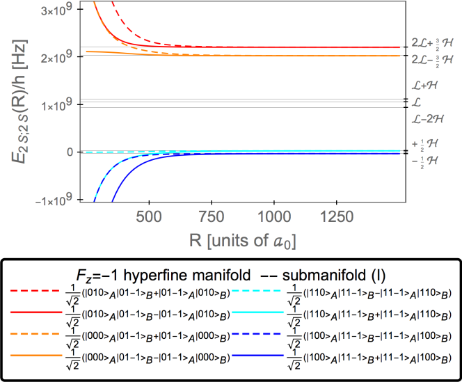
Figure 9: (Color online.) Evolution of the energy levels of the submanifold $\mathrm{\@slowromancap i@}$ within the $F_{z}=-1$ hyperfine manifold as a function of interatomic separation. The eigenstates given in the legend are only asymptotic, for finite separation these states mix.

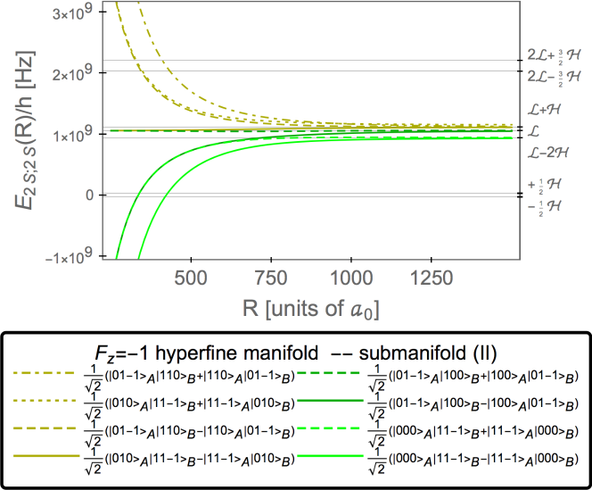
Figure 10: (Color online.) Evolution of the energy levels of the submanifold $\mathrm{\@slowromancap ii@}$ within the $F_{z}=-1$ hyperfine manifold as a function of interatomic separation. The eigenstates given in the legend are only asymptotic, for finite separation these states mix. The curve for the seventh state in the legend (counted from the top) has been slightly offset for better readability, in actuality it is virtually indistinguishable from that for the sixth state.

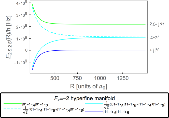
Figure 11: (Color online.) Evolution of the energy levels within the $F_{z}=-2$ hyperfine manifold as a function of interatomic separation. The eigenstates given in the legend are only asymptotic, for finite separation these states mix.

The dipole-dipole interaction results in level crossings (see Figs. 4—10), which is a feature of the hyperfine-resolved treatment of the problem. We are able to confirm that, in the coarse-structure limit ${\mathcal{L}}\rightarrow 0$, $\mathcal{F}\rightarrow 0$, no such level crossings are present (as found in Ref. Jonsell et al. (2002)). We note that, in the hyperfine resolved problem, there are no level crossings for the $F_{z}=\pm 2$ manifolds (see Figs. 1 and 11); for the $F_{z}=\pm 1$ manifolds, only crossings between levels belonging to different irreducible submanifolds take place (in other words, the energies of states which are asymptotically of the $2S$–$2P$ type on the one side, and of states of the $2S$–$2S$ and $2P$–$2P$ type on the other, cross for $R<500\,a_{0}$, see Figs. 2, 3, 9 and 10); while, for the $F_{z}=0$ manifold, both intra-submanifold (for $R<1\,000\,a_{0}$) and inter-submanifold (for $R<500\,a_{0}$) level crossings take place (see Figs. 4, 5, 6, 7 and 8).

Of particular phenomenological interest are the $2S$ hyperfine singlet to hyperfine triplet transitions with $|(0,0,0)_{A}\rangle\to|(0,1,0)_{A}\rangle$ with the spectator atom $B$ in a specific state. We find that all transitions with the spectator atom in a $P$ state undergo first-order van der Waals shifts (of order $1/R^{3}$), while the shift is of order $1/R^{6}$ if the spectator atom is in an $S$ state, that is, of second order in ${\mathcal{V}}$. This is due to the fact that $2S$–$2S$ states are not coupled to energetically degenerate states (they are only coupled to $2P$–$2P$ states), while $2S$–$2P$ states are coupled to $2P$–$2S$ states with which they are energetically degenerate. In other words, these different behaviors are ultimately due to the selection rules. The spectator atom in a $P$ state, however, decays very fast to the ground state by one-photon emission, with a lifetime of approximately $1.60\times 10^{-9}\,\mathrm{s}$ Bethe and Salpeter (1957), so that, depending on the exact experimental setup, the large van der Waals interaction energy shifts of the $2S(F=0)\to 2S(F=1)$ hyperfine transition (with the spectator atom being in a $2P$ state) do not play a role in the analysis of atomic beam experiments. Otherwise, we observe that a spectator atom in a $P$ state induces larger frequency shifts, comparing, e.g., the shifts in Tables 1 and 2 for $R=750\,a_{0}$ and $R=500\,a_{0}$.

As shown in Sec. IV, the precise numerical coefficients of the van der Waals shifts of the hyperfine singlet to hyperfine triplet transitions $|(0,0,0)_{A}\rangle\to|(0,1,0)_{A}\rangle$ depend on the symmetry of the wave function superposition of atoms $A$ and $B$, and cannot be uniquely expressed in terms of a specific state of the spectator atom $B$ alone; a symmetrization term is required [see the term prefixed with $\pm$ in Eqs. (108), (110) and (117), the same is true in the $F_{z}=-1$ subspace]. For spectroscopy, one essential piece of information to be derived from the results given in Eqs. (108), (110), (117) and (121) is that the van der Waals interaction energy shift for $2S(F=0)\to 2S(F=1)$ hyperfine transitions (with the spectator atom in a metastable $2S$ state) is of order ${\mathcal{V}}^{2}/{\mathcal{L}}$, where the parameters are defined in Eq. (15) [see also the remark in the text following Eq. (123)]. It is straightforward to see from Eq. (15c) that, for interatomic separation $R\sim 5\times 10^{5}\,a_{0}\simeq 2.6\times 10^{-5}\,\mathrm{m}$, the van der Waals shift reaches the experimental accuracy of the $2S$ hyperfine frequency measurements Kolachevsky et al. (2009).

Expressed more conveniently, still in SI mksA units, the shift is of order

$$E_{2S;2S}(R)\sim\frac{{\mathcal{V}}^{2}}{{\mathcal{L}}}\sim E_{h}\left(\frac{a_{0}}{R}\right)^{6}\,\frac{E_{h}}{{\mathcal{L}}}$$ (126)

where $E_{h}$ is the Hartree energy, $a_{0}$ is the Bohr radius, and ${\mathcal{L}}\sim\alpha^{3}\,E_{h}$ is the Lamb shift energy [see Eq. (3)].

A quick word is in order about how the present results can be transposed to hydrogen-like systems such as positronium and muonium. For positronium, the hierarchy between the fine structure, Lamb shift and hyperfine structure is not the same as that for hydrogen, so that the treatment used here; based on that hierarchy, does not apply. For muonium, on the other hand, our analysis remains relevant. Given that the reduced mass for the muonium system is very close to that of the hydrogen atom, the fine structure and Lamb shift-type splittings are almost identical to those of hydrogen. The hyperfine splitting is $(g_{s}/g_{N})\,(m_{p}/m_{\mu})\sim 3.2$ times larger than that of atomic hydrogen. Finally, given the close proximity of the reduced masses, muonium has a Bohr radius very close to that of hydrogen, so that the intensity of the dipole-dipole interactions will be essentially identical, for equal separations, between two hydrogen atoms and between two muonium atoms.

In this work as well as in the previous paper Adhikari et al. (2017) of this series, we have treated dipole-dipole interactions between atoms sitting in $S$ states (though, in the present case, we had to treat the $2P_{1/2}$ state on the same footing as $2S$, given their quasi-degeneracy). Finally, we should comment on the distance range for which our calculations remain applicable. We have used the nonretardation approximation in Eq. (2c). For the $2S$–$2S$ interaction via adjacent $2P_{1/2}$ states, retardation sets in when the phase of the atomic oscillation during a virtual (Lamb shift) transition changes appreciably on the time scale it takes light to travel the interatomic separation distance $R$, i.e., when

$$\frac{R}{c}\sim\frac{\hbar}{{\mathcal{L}}}\,.$$ (127)

We have $R\sim\hbar c/{\mathcal{L}}$ when $R$ is on the order of the Lamb shift wavelength of about $30\,{\rm cm}$. The nonretardation approximation thus is valid over all distance ranges of physical interest, for the ($2S$;$2S$)-system.

Appendix A Further Manifolds

A.1 Manifold $\maybebm{F_{z}=-1}$

We can identify two irreducible subspaces within the $F_{z}=-1$ manifold: the subspace $\mathrm{\@slowromancap i@}$ composed of the states

$$|\psi_{1}^{\prime\left(\mathrm{\@slowromancap i@}\right)}\rangle= \;|(0,0,0)_{A}\,(0,1,-1)_{B}\rangle\,,\qquad|\psi_{2}^{\prime\left(\mathrm{\@slowromancap i@}\right)}\rangle=|(0,1,-1)_{A}\,(0,0,0)_{B}\rangle\,,\qquad|\psi_{3}^{\prime\left(\mathrm{\@slowromancap i@}\right)}\rangle=|(0,1,-1)_{A}\,(0,1,0)_{B}\rangle\,,$$ (128)

$$|\psi_{4}^{\prime\left(\mathrm{\@slowromancap i@}\right)}\rangle= \;|(0,1,0)_{A}\,(0,1,-1)_{B}\rangle\,,\qquad|\psi_{5}^{\prime\left(\mathrm{\@slowromancap i@}\right)}\rangle=\;|(1,0,0)_{A}\,(1,1,-1)_{B}\rangle\,,\qquad|\psi_{6}^{\prime\left(\mathrm{\@slowromancap i@}\right)}\rangle=|(1,1,-1)_{A}\,(1,0,0)_{B}\rangle\,,$$

$$|\psi_{7}^{\prime\left(\mathrm{\@slowromancap i@}\right)}\rangle= \;|(1,1,-1)_{A}\,(1,1,0)_{B}\rangle\,,\qquad|\psi_{8}^{\prime\left(\mathrm{\@slowromancap i@}\right)}\rangle=|(1,1,0)_{A}\,(1,1,-1)_{B}\rangle\,$$

where the Hamiltonian matrix reads

$$H_{F_{z}=-1}^{\prime\left(\mathrm{\@slowromancap i@}\right)}= \;\left(\begin{array}[]{cccccccc}2{\mathcal{L}}-\tfrac{3}{2}{\mathcal{H}}&0&0&0&0&{\mathcal{V}}&{\mathcal{V}}&2{\mathcal{V}}\\ 0&2{\mathcal{L}}-\tfrac{3}{2}{\mathcal{H}}&0&0&{\mathcal{V}}&0&2{\mathcal{V}}&{\mathcal{V}}\\ 0&0&2{\mathcal{L}}+\tfrac{3}{2}{\mathcal{H}}&0&{\mathcal{V}}&2{\mathcal{V}}&0&{\mathcal{V}}\\ 0&0&0&2{\mathcal{L}}+\tfrac{3}{2}{\mathcal{H}}&2{\mathcal{V}}&{\mathcal{V}}&{\mathcal{V}}&0\\ 0&{\mathcal{V}}&{\mathcal{V}}&2{\mathcal{V}}&-\tfrac{1}{2}{\mathcal{H}}&0&0&0\\ {\mathcal{V}}&0&2{\mathcal{V}}&{\mathcal{V}}&0&-\tfrac{1}{2}{\mathcal{H}}&0&0\\ {\mathcal{V}}&2{\mathcal{V}}&0&{\mathcal{V}}&0&0&\tfrac{1}{2}{\mathcal{H}}&0\\ 2{\mathcal{V}}&\mathcal{V}&{\mathcal{V}}&0&0&0&0&\tfrac{1}{2}{\mathcal{H}}\end{array}\right)\,,$$ (137)

and the subspace $\mathrm{\@slowromancap ii@}$ composed of the states

$$|\psi_{1}^{\prime\left(\mathrm{\@slowromancap ii@}\right)}\rangle= \;|(0,0,0)_{A}\,(1,1,-1)_{B}\rangle\,,\qquad|\psi_{2}^{\prime\left(\mathrm{\@slowromancap ii@}\right)}\rangle=|(0,1,-1)_{A}\,(1,0,0)_{B}\rangle\,,\qquad|\psi_{3}^{\prime\left(\mathrm{\@slowromancap ii@}\right)}\rangle=|(0,1,-1)_{A}\,(1,1,0)_{B}\rangle\,,$$ (138)

$$|\psi_{4}^{\prime\left(\mathrm{\@slowromancap ii@}\right)}\rangle= \;|(0,1,0)_{A}\,(1,1,-1)_{B}\rangle\,,\qquad|\psi_{5}^{\prime\left(\mathrm{\@slowromancap ii@}\right)}\rangle=|(1,0,0)_{A}\,(0,1,-1)_{B}\rangle\,,\qquad|\psi_{6}^{\prime\left(\mathrm{\@slowromancap ii@}\right)}\rangle=|(1,1,-1)_{A}\,(0,0,0)_{B}\rangle\,,$$

$$|\psi_{7}^{\prime\left(\mathrm{\@slowromancap ii@}\right)}\rangle= \;|(1,1,-1)_{A}\,(0,1,0)_{B}\rangle\,,\qquad|\psi_{8}^{\prime\left(\mathrm{\@slowromancap ii@}\right)}\rangle=|(1,1,0)_{A}\,(0,1,-1)_{B}\rangle\,,$$

where the Hamiltonian matrix reads

$$H_{F_{z}=-1}^{\left(\mathrm{\@slowromancap ii@}\right)}= \;\left(\begin{array}[]{cccccccc}{\mathcal{L}}-2{\mathcal{H}}&0&0&0&0&{\mathcal{V}}&{\mathcal{V}}&2{\mathcal{V}}\\ 0&{\mathcal{L}}&0&0&{\mathcal{V}}&0&2{\mathcal{V}}&{\mathcal{V}}\\ 0&0&{\mathcal{L}}+{\mathcal{H}}&0&{\mathcal{V}}&2{\mathcal{V}}&0&{\mathcal{V}}\\ 0&0&0&{\mathcal{L}}+{\mathcal{H}}&2{\mathcal{V}}&{\mathcal{V}}&{\mathcal{V}}&0\\ 0&{\mathcal{V}}&{\mathcal{V}}&2{\mathcal{V}}&{\mathcal{L}}&0&0&0\\ {\mathcal{V}}&0&2{\mathcal{V}}&{\mathcal{V}}&0&{\mathcal{L}}-2{\mathcal{H}}&0&0\\ {\mathcal{V}}&2{\mathcal{V}}&0&{\mathcal{V}}&0&0&{\mathcal{L}}+{\mathcal{H}}&0\\ 2{\mathcal{V}}&\mathcal{V}&{\mathcal{V}}&0&0&0&0&{\mathcal{L}}+{\mathcal{H}}\end{array}\right).$$ (147)

Surprisingly, the Hamiltonian matrix is a little different from the case with $F_{z}=+1$, even if one reorders the basis vectors accordingly. The energy eigenvalues of course are the same.

Again within the $\mathrm{\@slowromancap i@}$ subspace there are no degenerate subspaces with nonzero coupling, while, in the $\mathrm{\@slowromancap ii@}$ subspace we can identify degenerate states coupled to each other. The analysis carried out in Sec. III.2 applies here if we make the following substitutions:

$$|\psi_{1}^{\left(\mathrm{\@slowromancap ii@}\right)}\rangle \rightarrow|\psi_{1}^{\prime\left(\mathrm{\@slowromancap ii@}\right)}\rangle\,,\;\;|\psi_{2}^{\left(\mathrm{\@slowromancap ii@}\right)}\rangle\rightarrow|\psi_{3}^{\prime\left(\mathrm{\@slowromancap ii@}\right)}\rangle\,,\;\;|\psi_{3}^{\left(\mathrm{\@slowromancap ii@}\right)}\rangle\rightarrow|\psi_{4}^{\prime\left(\mathrm{\@slowromancap ii@}\right)}\rangle\,,$$ (148)

$$|\psi_{4}^{\left(\mathrm{\@slowromancap ii@}\right)}\rangle \rightarrow|\psi_{2}^{\prime\left(\mathrm{\@slowromancap ii@}\right)}\rangle\,,\;\;|\psi_{5}^{\left(\mathrm{\@slowromancap ii@}\right)}\rangle\rightarrow|\psi_{5}^{\prime\left(\mathrm{\@slowromancap ii@}\right)}\rangle\,,\;\;|\psi_{6}^{\left(\mathrm{\@slowromancap ii@}\right)}\rangle\rightarrow|\psi_{7}^{\prime\left(\mathrm{\@slowromancap ii@}\right)}\rangle\,,$$

$$|\psi_{7}^{\left(\mathrm{\@slowromancap ii@}\right)}\rangle \rightarrow|\psi_{8}^{\prime\left(\mathrm{\@slowromancap ii@}\right)}\rangle\,,\;\;|\psi_{8}^{\left(\mathrm{\@slowromancap ii@}\right)}\rangle\rightarrow|\psi_{6}^{\prime\left(\mathrm{\@slowromancap ii@}\right)}\rangle\,,$$

so that we need not go over the analysis of degenerate subspaces again. (Even when making this reordering, many off-diagonal terms have different signs in $H_{F_{z}=+1}^{\left(\mathrm{\@slowromancap ii@}\right)}$ and $H_{F_{z}=-1}^{\left(\mathrm{\@slowromancap ii@}\right)}$. But only the couplings between non-degenerate states have different signs, while coupling between degenerate states remain identical. This latter point means that the analysis of Sec. III.2 also applies to $H_{F_{z}=-1}^{\left(\mathrm{\@slowromancap ii@}\right)}$.) However, for the sake of completeness and clarity, in Figs. 9 and 10, we plot the evolution of the eigenvalues with respect to interatomic separation. Notice that the evolution of the energy eigenstates is identical to the eigenstates in the $F_{z}=+1$ manifold.

A.2 Manifold $\maybebm{F_{z}=-2}$

We can identify two irreducible subspaces within the $F_{z}=+2$ manifold: the subspace $\mathrm{\@slowromancap i@}$ composed of the states

$$|\phi_{1}^{\prime\left(\mathrm{\@slowromancap i@}\right)}\rangle =|(0,1,-1)_{A}\,(0,1,-1)_{B}\rangle\,,$$ (149)

$$|\phi_{2}^{\prime\left(\mathrm{\@slowromancap i@}\right)}\rangle =|(1,1,-1)_{A}\,(1,1,-1)_{B}\rangle\,,$$ (150)

where the Hamiltonian matrix reads

$$H_{F_{z}=-2}^{\left(\mathrm{\@slowromancap i@}\right)}=\left(\begin{array}[]{cc}2{\mathcal{L}}+\tfrac{3}{2}{\mathcal{H}}&-2{\mathcal{V}}\\ -2{\mathcal{V}}&\tfrac{1}{2}{\mathcal{H}}\\ \end{array}\right)\,,$$ (151)

and the subspace $\mathrm{\@slowromancap ii@}$ is composed of the states

$$|\phi_{1}^{\prime\left(\mathrm{\@slowromancap ii@}\right)}\rangle =|(0,1,-1)_{A}\,(1,1,-1)_{B}\rangle\,,$$ (152)

$$|\phi_{2}^{\prime\left(\mathrm{\@slowromancap ii@}\right)}\rangle =|(1,1,-1)_{A}\,(0,1,-1)_{B}\rangle\,,$$ (153)

where the Hamiltonian matrix reads

$$H_{F_{z}=-2}^{\left(\mathrm{\@slowromancap ii@}\right)}=\left(\begin{array}[]{cccc}{\mathcal{L}}+{\mathcal{H}}&-2{\mathcal{V}}\\ -2{\mathcal{V}}&{\mathcal{L}}+{\mathcal{H}}\\ \end{array}\right)\,.$$ (154)

We do not repeat the analysis of the eigensystem and refer the reader to Sec. III.1. The results given there are immediately transposed to the present case, by the simple substitution $|\phi_{i}\rangle\rightarrow|\phi^{\prime}_{i}\rangle$. However, for the sake of completeness and clarity, in Fig. 11, we still plot the evolution of the eigenvalues with respect to interatomic separation. Notice that the evolution of the energy eigenstates is identical to the eigenstates in the $F_{z}=+2$ manifold.

References

- Kolachevsky et al. (2009) N. Kolachevsky, A. Matveev, J. Alnis, C. G. Parthey, S. G. Karshenboim, and T. W. Hänsch, “Measurement of the Hyperfine Interval in Atomic Hydrogen,” Phys. Rev. Lett. 102, 213002 (2009).
- Adhikari et al. (2017) C. M. Adhikari, V. Debierre, A. Matveev, N. Kolachevsky, and U. D. Jentschura, Long-range interactions of hydrogen atoms in excited states. I. – interactions and Dirac– perturbations, accepted for publication in Physical Review A (2017).
- Jonsell et al. (2002) S. Jonsell, A. Saenz, P. Froelich, R. C. Forrey, R. Côté, and A. Dalgarno, “Long-range interactions between two 2s excited hydrogen atoms,” Phys. Rev. A 65, 042501 (2002).
- Simonsen et al. (2011) S. I. Simonsen, L. Kocbach, and J. P. Hansen, “Long-range interactions and state characteristics of interacting Rydberg atoms,” J. Phys. B 44, 165001 (2011).
- Note (1) More accurately, the conclusions of Ref. Jonsell et al. (2002) announce a future work where “the effects of spin-orbit coupling and the Lamb shift” would be taken into account. As far as we could find, no such work has been published yet.
- Ray et al. (1968a) S. Ray, J. D. Lyons, and T. P. Das, “Hyperfine Pressure Shift and van der Waals Interactions. I. Hydrogen–Helium System,” Phys. Rev. 174, 104–112 (1968a), erratum Phys. Rev. 181, 465 (1969)].
- Ray et al. (1968b) S. Ray, J. D. Lyons, and T. P. Das, “Hyperfine Pressure Shift and van der Waals Interactions. II. Nitrogen–Helium System,” Phys. Rev. 174, 112–118 (1968b), erratum Phys. Rev. 181, 465 (1969)].
- Rao and Das (1969) B. K. Rao and T. P. Das, “Hyperfine Pressure Shift and van der Waals Interactions. III. Temperature Dependence,” Phys. Rev. 185, 95–97 (1969).
- Rao and Das (1970) B. K. Rao and T. P. Das, “Hyperfine Pressure Shift and van der Waals Interactions. IV. Hydrogen–Rare–Gas Systems,” Phys. Rev. A 2, 1411–1421 (1970).
- Pachucki (2005) K. Pachucki, “Relativistic corrections to the long-range interaction between closed-shell atoms,” Phys. Rev. A 72, 062706 (2005).
- Itzykson and Zuber (1980) C. Itzykson and J. B. Zuber, Quantum Field Theory (McGraw-Hill, New York, 1980).
- Lundeen and Pipkin (1981) S. R. Lundeen and F. M. Pipkin, “Measurement of the Lamb Shift in Hydrogen, ,” Phys. Rev. Lett. 46, 232–235 (1981).
- Jentschura and Yerokhin (2006) U. D. Jentschura and V. A. Yerokhin, “Quantum electrodynamic corrections to the hyperfine structure of excited states,” Phys. Rev. A 73, 062503 (2006).
- Varshalovich et al. (1988) D. A. Varshalovich, A. N. Moskalev, and V. K. Khersonskii, Quantum Theory of Angular Momentum (World Scientific, Singapore, 1988).
- Bethe and Salpeter (1957) H. A. Bethe and E. E. Salpeter, Quantum Mechanics of One- and Two-Electron Atoms (Springer, Berlin, 1957).