Long-range interactions of hydrogen atoms in excited states. I.
$\bm{2S}$ $\bm{1S}$ interactions and Dirac–$\bm{\delta}$ perturbations

C. M. Adhikari Department of Physics, Missouri University of Science and Technology, Rolla, Missouri 65409-0640, USA    V. Debierre Department of Physics, Missouri University of Science and Technology, Rolla, Missouri 65409-0640, USA    A. Matveev P. N. Lebedev Physics Institute, Leninsky prosp. 53, Moscow, 119991 Russia Max–Planck–Institut für Quantenoptik, Hans–Kopfermann-Straße 1, 85748 Garching, Germany    N. Kolachevsky P. N. Lebedev Physics Institute, Leninsky prosp. 53, Moscow, 119991 Russia Max–Planck–Institut für Quantenoptik, Hans–Kopfermann-Straße 1, 85748 Garching, Germany Russian Quantum Center, Business-center “Ural”, 100A Novaya street, Skolkovo, Moscow, 143025 Russia    U. D. Jentschura Department of Physics, Missouri University of Science and Technology, Rolla, Missouri 65409-0640, USA
Abstract

The theory of the long-range interaction of metastable excited atomic states with ground-state atoms is analyzed. We show that the long-range interaction is essentially modified when quasi-degenerate states are available for virtual transitions. A discrepancy in the literature regarding the van der Waals coefficient $C_{6}(2S;1S)$ describing the interaction of metastable atomic hydrogen ($2S$ state) with a ground-state hydrogen atom is resolved. In the the van der Waals range $a_{0}\ll R\ll a_{0}/\alpha$, where $a_{0}=\hbar/(\alpha mc)$ is the Bohr radius and $\alpha$ is the fine structure constant, one finds the symmetry-dependent result $E_{2S;1S}(R)\approx(-176.75\pm 27.98)\,E_{h}\,(a_{0}/R)^{6}$ ($E_{h}$ denotes the Hartree energy). In the Casimir–Polder range $a_{0}/\alpha\ll R\ll\hbar c/{\mathcal{L}}$, where ${\mathcal{L}}\equiv E\left(2S_{1/2}\right)-E\left(2P_{1/2}\right)$ is the Lamb shift energy, one finds $E_{2S;1S}(R)\approx(-121.50\pm 46.61)\,E_{h}\,(a_{0}/R)^{6}$. In the the Lamb shift range $R\gg\hbar c/{\cal L}$, we find an oscillatory tail with a negligible interaction energy below $10^{-36}\,{\rm Hz}$. Dirac–$\delta$ perturbations to the interaction are also evaluated and results are given for all asymptotic distance ranges; these effects describe the hyperfine modification of the interaction, or, expressed differently, the shift of the hydrogen $2S$ hyperfine frequency due to interactions with neighboring $1S$ atoms. The $2S$ hyperfine frequency has recently been measured very accurately in atomic beam experiments.

pacs:
31.30.jh, 31.30.J-, 31.30.jf

I Introduction

The purpose of this paper is twofold. First, we aim to revisit the calculation of the long-range (van der Waals and Casimir–Polder interaction) for ground-state hydrogen interacting with an excited-state atom in an $2S$ state. Second, we aim to study the perturbation of the van der Waals interactions by a Dirac-$\delta$ potential perturbing the metastable excited state which participates in the interaction. Such a Dirac-$\delta$ potential can be due to the electron-nucleus (hyperfine) interaction in one of the atoms Jentschura and Yerokhin (2006) or due to a self-energy radiative correction Bethe (1947). Special emphasis is laid on the role of quasi-degenerate levels and on the exchange term, which is due to the possibility of $1S$ $2S$ atoms becoming a $2S$ $1S$ pair after the exchange of two virtual photons Chibisov (1972).

It is interesting to notice that two results given in the literature for the so-called van der Waals coefficient of the $1/R^{6}$ nonretarded interaction between $1S$ and $2S$ states, are in significant mutual disagreement (numerically, the authors of Refs. Deal and Young (1973) obtain a value of roughly $177$ in atomic units, while a result of about $57$ has been derived in Refs. Chibisov (1972); Tang and Chan (1986)). We attempt a thorough analysis of the discrepancy. Two different methods of calculation were employed in Ref. Deal and Young (1973) (direct sum over virtual atomic states, including the continuum) and Refs. Chibisov (1972); Tang and Chan (1986) (integration over analytic expressions representing the polarizability).

The role of the virtual, quasi-degenerate $2P$ states deserves special attention. For $2S$ reference states, the $2P_{1/2}$ and $2P_{3/2}$ levels are displaced only by the Lamb shift and fine structure, respectively. Significant modifications of the long-range interactions result from the presence of the quasi-degenerate states.

Recently, precision measurements of the $2S$ hyperfine splitting have been carried out using an atomic beam consisting of a mixture of ground-state $1S$ hydrogen atoms, and metastable $2S$ atoms Kolachevsky et al. (2004, 2009). To leading order, the van der Waals interaction shifts all hyperfine structure components equally. However, there is a correction to the van der Waals interaction due to the the hyperfine structure (HFS), which depends on the total (electron$+$nucleus) angular momentum quantum number $F$. This correction shifts HFS components closer to each other. This latter effect is analyzed in the current paper; it is of phenomenological significance because of van der Waals interactions inside the atomic beam. Again, special attention is required in the treatment of the quasi-degenerate atomic levels.

Let us recall here that the general subject of long-range interactions of simple atoms is very well known to the physics community, and a few investigations on simple atomic systems can be found in Refs. Dalgarno and Davidson (1966); Dalgarno (1967); Ray et al. (1968a, b); Rao and Das (1969, 1970); Dalgarno et al. (1968); Dutta et al. (1970); Deal and Young (1973); Tang and Chan (1986); Yan et al. (1996, 1997). Various aspects of the problem have been studied in depth: e.g., the importance of multipole mixing effects, and of perturbations by hyperfine effects, has been stressed in Ref. Ray et al. (1968a, b); Rao and Das (1969, 1970). Higher-order effects such as dipole-octupole mixing terms were discussed in detail for hydrogen in Ref. Tang and Chan (1986) and for helium in Ref. Yan et al. (1996). The dipole-dipole interaction potential of helium, including retardation, has been discussed in great detail in Refs. Jamieson et al. (1995); Chen and Chung (1996), including a number of numerical examples. More complex alkali-metal dimers have been considered in Refs. Marinescu et al. (1994); Marinescu and Dalgarno (1995).

Throughout this article, we work in SI mksA units and keep all factors of $\hbar$ and $c$ in the formulas. With this choice, we attempt to enhance the accessibility of the presentation to two different communities, namely, the quantum electrodynamics (QED) community which in general uses the natural unit system, and the atomic physics community where the atomic unit system is canonically employed. In the former, one sets $\hbar=c=\epsilon_{0}=1$, and the electron mass is denoted as $m$. The relation $e^{2}=4\pi\alpha$ then allows to identify the expansion in the number of quantum electrodynamic corrections with powers of the fine structure constant $\alpha\approx 1/137.036$. This unit system is used, e.g., in the investigation reported in Ref. Pachucki (2005) on relativistic corrections to the Casimir–Polder interaction (with a strong overlap with QED). In the atomic unit system, we have $\left|e\right|=\hbar=m=1$, and $4\pi\epsilon_{0}=1$. The speed of light, in the atomic unit system, is $c=1/\alpha\approx 137.036$. This system of units is especially useful for the analysis of purely atomic properties without radiative effects. As the subject of the current study lies in between the two mentioned fields of interest, we choose the SI unit system as the most appropriate reference frame for our calculations. The formulas do not become unnecessarily complex, and can be evaluated with ease for any experimental application.

We organize this paper as follows. The problem is somewhat involved, as such, we attempt to orient ourselves in Sec. II. The direct term in the $2S$ $1S$ interaction is analyzed in Sec. III. In Sec. III.2, we study that interaction in the van der Waals range. The very-large-distance limit is discussed in Sec. III.3 (atomic distance larger than the wavelength of the Lamb shift transition), and the intermediate Casimir–Polder range in Sec. III.4. The mixing term in the $2S$ $1S$ interaction is analyzed in Sec. IV. We then analyze a Dirac-$\delta$ (HFS induced) induced modification both for the $2S$ $1S$ interaction as well as for the $1S$ $1S$ interaction in Sec. V. In Sec. VI, we numerically evaluate the shift of the $2S$ hyperfine frequency due to the long-range interaction with a ground state hydrogen atom. Conclusions are drawn in Sec. VII.

II Orientation

In order to evaluate the van der Waals correction to the $2S$ $1S$ hyperfine frequency, one needs to diagonalize the total Hamiltonian

$$H_{\rm total}=H_{S}+H_{\rm FS}+H_{\rm LS}+H_{\rm HFS}+H_{\rm vdW}\,.$$ (1)

Here, $H_{S}$ is the Schrödinger Hamiltonian, $H_{\rm FS}$ is the fine structure Hamiltonian, which can be approximated as (see Chap. 34 of Ref. Berestetskii et al. (1982))

$\displaystyle H_{\rm FS}=$ $\displaystyle\;\sum_{i=A,B}\left[-\frac{\vec{p}_{i}^{\,4}}{8m^{3}c^{2}}+\frac{1}{2}\alpha\left(\frac{\hbar^{2}g_{s}}{2m^{2}\,c}\right)\frac{\vec{L}_{i}\cdot\vec{S}_{i}}{|\vec{r}_{i}|^{3}}\right.$
$\displaystyle\;\left.+\frac{\hbar^{3}}{8m^{2}c}\,4\pi\alpha\,\delta^{(3)}(\vec{r}_{i})\right],$ (2)

where $m$ is the electron mass, the $\vec{p}_{i}$ denote the momenta of the two atomic electrons relative to their nuclei ($i$ runs over the atoms $A$ and $B$), and the $\vec{r}_{i}=\vec{x}_{i}-\vec{R}_{i}$ denote the coordinates relative to the nuclei (the electron and nucleus coordinates are $\vec{x}_{i}$ and $\vec{R}_{i}$, respectively). We restrict the discussion to neutral hydrogen atoms and thus assume a nuclear charge number of $Z=1$. We shall use the following approximation to the “Lamb shift Hamiltonian”, which constitutes an effective Hamiltonian useful in the evaluation of the leading radiative correction to dynamic processes Karshenboim and Ivanov (1997); Jentschura (2004),

$$H_{\mathrm{LS}}=\sum_{i=A,B}\frac{4}{3}\,\alpha^{2}mc^{2}\left(\frac{\hbar}{mc}\right)^{3}\ln\left(\alpha^{-2}\right)\,\delta^{\left(3\right)}\left(\vec{r}_{i}\right)\,.$$ (3)

We shall use this Hamiltonian later in the analysis of the radiative correction to the long-range interatomic interaction. The Hamiltonian for the hyperfine interaction Itzykson and Zuber (1980); Jentschura and Yerokhin (2006) reads as

$\displaystyle H_{\rm HFS}=$ $\displaystyle\;\frac{\mu_{0}}{4\pi}\;\mu_{B}\,\mu_{N}\,g_{s}\,g_{p}\sum_{i=A,B}\left[\frac{8\pi}{3}\,\vec{S}_{i}\cdot\vec{I}_{i}\,\delta^{(3)}(\vec{r}_{i})\right.$
$\displaystyle\;\left.+\frac{3\,(\vec{S}_{i}\cdot\hat{r}_{i})(\vec{I}_{i}\cdot\hat{r}_{i})-(\vec{S}_{i}\cdot\vec{I}_{i})}{|\vec{r}_{i}|^{3}}+\frac{\vec{L}_{i}\cdot\vec{\mu}_{i}}{\hbar|\vec{r}_{i}|^{3}}\right]\,.$ (4)

Here, the unit vectors are $\hat{r}_{i}=\vec{r}_{i}/|\vec{r}_{i}|$. The spin operator for the electron $i$ is $\vec{S}_{i}=\vec{\sigma}_{i}/2$, while $\vec{I}_{i}$ is the spin operator for proton $i$ (both spin operators are dimensionless). The electronic and protonic $g$ factors are $g_{s}\simeq 2.002\,319$ and $g_{p}\simeq 5.585\,695$, while $\mu_{B}\simeq 9.274\,010\,\times 10^{-24}\,\mathrm{Am}^{2}$ is the Bohr magneton and $\mu_{N}\simeq 5.050\,784\,\times 10^{-27}\,\mathrm{Am}^{2}$ is the nuclear magneton Mohr et al. (2012). It is well known that, for $S$ states, the second term in the fine structure Hamiltonian (II), and the second and third terms in the hyperfine structure Hamiltonian (II) have vanishing contributions. For $S$ states, the relevant term in the hyperfine Hamiltonian therefore is of the Dirac-$\delta$ type. Hence, we put special emphasis on the modifications occasioned by such Dirac-$\delta$ potentials.

The van der Waals energy is normally derived as follows. One first writes the attractive and repulsive terms that describe the electron-electron, electron-proton, and proton-proton interactions in the two atoms (excluding the intra-atomic terms). This leads to the total Coulomb interaction

$\displaystyle V_{\mathrm{C}}$ $\displaystyle=\frac{e^{2}}{4\pi\epsilon_{0}}\left(\frac{1}{|\vec{R}_{A}-\vec{R}_{B}|}+\frac{1}{\left|\vec{x}_{A}-\vec{x}_{B}\right|}\right.$ (5)
$\displaystyle\;\left.-\frac{1}{|\vec{x}_{A}-\vec{R}_{B}|}-\frac{1}{|\vec{x}_{B}-\vec{R}_{A}|}\right)\,.$

One then uses the fact that the separation $|\vec{R}_{A}-\vec{R}_{B}|$ between the two nuclei (protons) is much larger than that between a given proton and its respective electron, that is, much larger than both $|\vec{r}_{A}|=|\vec{x}_{A}-\vec{R}_{A}|$ and $|\vec{r}_{B}|=|\vec{x}_{B}-\vec{R}_{B}|$. One then writes $\vec{x}_{A}-\vec{R}_{B}=\vec{r}_{A}+(\vec{R}_{A}-\vec{R}_{B})$ and $\vec{x}_{B}-\vec{R}_{A}=\vec{r}_{B}+(\vec{R}_{B}-\vec{R}_{A})$. Expanding in $\vec{r}_{A}$ and $\vec{r}_{B}$, one obtains

$\displaystyle H_{\rm vdW}=$ $\displaystyle\;\frac{e^{2}}{4\pi\epsilon_{0}}\,\frac{\vec{r}_{A}\cdot\vec{r}_{B}-3\,(\vec{r}_{A}\cdot\hat{R})\,(\vec{r}_{B}\cdot\hat{R})}{R^{3}}$
$\displaystyle=$ $\displaystyle\;\frac{e^{2}}{4\pi\epsilon_{0}\,R^{3}}\,\left(\delta_{k\ell}-3\,\hat{R}_{k}\hat{R}_{\ell}\right)r_{Ak}\,r_{B\ell}\,,$ (6)

where $\vec{R}=\vec{R}_{A}-\vec{R}_{B}$, $R=|\vec{R}|$ and $\hat{R}=\vec{R}/R$. The indices $k$ and $\ell$ corresponding to the Cartesian coordinates are summed over (Einstein summation convention). The van der Waals interaction term, for a $2S$ $1S$ system, has vanishing elements in first-order perturbation theory. Both atoms $A$ and $B$ have to undergo a virtual dipole transition to a $P$ state for a nonvanishing effect, and the leading-order van der Waals interaction is obtained in second-order perturbation theory, leading to a $1/R^{6}$ interaction energy. The propagator denominator in the standard Rayleigh–Schrödinger expression for the second-order energy shift due to $H_{\rm vdW}$ is equal to the sum of the virtual excitation energies of both atoms Deal and Young (1973). The close-range asymptotics of the interatomic interaction energy thus goes as $1/R^{6}$ Deal and Young (1973). For an interatomic distance of $R\sim 30a_{0}\ldots 100\,a_{0}$ (one hundred atomic units), the energy shift is on the order of $10^{-8}\ldots 10^{-12}$ atomic units (Hartrees). The hierarchy

$$\left<H_{\rm vdW}\right>\ll\left<H_{\rm HFS}\right>\ll\left<H_{\rm LS}\right>\ll\left<H_{\rm FS}\right>$$ (7)

is thus fulfilled for $R\gtrsim 30\,a_{0}$. For sufficiently large interatomic distance, the Dirac $\delta$ potential of the HFS acts as a perturbation and can be treated as such, and we shall focus on this regime in the current manuscript.

For clarity, we should point out that the Hamiltonian (II) remains valid in the nonretardation approximation. One can understand retardation as follows: When the phase of the atomic oscillation during a virtual transition changes appreciably on the time scale it takes light to travel the interatomic separation distance $R$, then the retarded form of the van der Waals interaction has to be used. The criterion for the validity of the nonretardation approximation thus is

$$\frac{R}{c}\ll\frac{\hbar}{E_{h}}=\frac{a_{0}}{\alpha\,c}\,,$$ (8)

or, more precisely,

$$a_{0}=\frac{\hbar}{\alpha mc}\ll R\ll\frac{\hbar}{\alpha^{2}mc}=\frac{a_{0}}{\alpha}\,,$$ (9)

if we take into account that substantial overlap of the electronic wavefunctions is to be avoided.

The retarded interatomic interaction cannot be obtained on the basis of Eq. (II) alone; one has to use the atom-field interaction term [see Eq. (85.4) of Ref. Berestetskii et al. (1982)],

$$V(t)=-\vec{E}(\vec{R}_{A},t)\cdot\vec{d}_{A}(t)-\vec{E}(\vec{R}_{B},t)\cdot\vec{d}_{B}(t)\,,$$ (10)

where $\vec{d}_{i}=e\,\vec{r}_{i}$ is the dipole operator for atom $i$ (for atoms with more than one electron, one has to sum over all the electrons in the atoms $i=A,B$). The $\vec{R}_{A}$ and $\vec{R}_{B}$ are the positions of the atomic nuclei, and $\vec{E}$ denotes the operator of the quantized electric field. An elegant way of deriving the retarded Casimir–Polder interaction, described in Eq. (85.4) of Ref. Berestetskii et al. (1982), then consists in the matching of the scattering amplitude obtained from quantum electrodynamics, against the effective interatomic interaction Hamiltonian. Alternative derivations use time-ordered perturbation theory Power and Thirunamachandran (1995).

The functional form of the interaction depends on the distance range In the van der Waals range (9) of interatomic distances, the interaction of ground-state atoms is of the usual $R^{-6}$ functional form. This remains valid if one atom is in a metastable excited state. In the so-called Casimir–Polder range,

$$R\gg\frac{\hbar}{\alpha^{2}mc}\,,$$ (11)

the interatomic distance is much larger than the wavelength of an optical transition, and the interaction of ground-state atoms has an $R^{-7}$ function form. For the long-range interaction involving excited metastable atoms, however, we have to distinguish a third range of very large interatomic distances,

$$\mbox{Casimir--Polder~{}II (or Lamb shift):}\quad R\gg\frac{\hbar c}{\cal L}\,,$$ (12)

which we would like to refer to as the Lamb shift range. Here, $\cal L$ is the Lamb shift energy. For metastable atoms, the Casimir–Polder range is bounded from above by the Lamb shift range, and the condition (11) should be modified to read

$$\mbox{Casimir--Polder~{}I:}\quad\frac{\hbar c}{\cal L}\gg R\gg\frac{\hbar}{\alpha^{2}mc}\,,$$ (13)

For the $1S$ $1S$ interaction, the interaction energy reaches the Casimir–Polder asymptotic form, proportional to $1/R^{7}$, in both regimes described by Eqs. (12) and (13). For the $2S$ $1S$ interaction, it is only in the very long-range regime (12) that we have a $R^{-7}$ interaction, with competing oscillatory terms Safari and Karimpour (2015); Donaire et al. (2015); Jentschura and Debierre (2016) proportional to $({\mathcal{L}}^{4}/R^{2})\cos[{\mathcal{L}}R/(\hbar c)]$.

A further complication arises. The state with atom $A$ in an excited state and atom $B$ in the ground state, $|2S\rangle_{A}\,|1S\rangle_{B}$, is degenerate with the state $|1S\rangle_{A}\,|2S\rangle_{B}$ with the quantum numbers reversed among the atoms. There is no direct first-order coupling between $|2S\rangle_{A}\,|1S\rangle_{B}$ and $|1S\rangle_{A}\,|2S\rangle_{B}$ due to the van der Waals interaction (II), but in second order, an off-diagonal term is obtained which is of the same order-of-magnitude as the diagonal term, i.e., the term with the same in and out states. The Hamiltonian matrix in the basis of the degenerate states $|2S\rangle_{A}\,|1S\rangle_{B}$ and $|1S\rangle_{A}\,|2S\rangle_{B}$ has off-diagonal (exchange) terms of second order in the van der Waals interaction Chibisov (1972). The energy eigenvalues and eigenstates are easily found in the degenerate basis and are studied here in Sec. IV.

III $\maybebm{2S}$ $\maybebm{1S}$ Direct Interaction

III.1 Formalism

According to Eq. (85.17) in Chap. 85 of Ref. Berestetskii et al. (1982), the interaction energy between two atoms $A$ and $B$ in states $\left|A\right>$ and $\left|B\right>$ is given by

$\displaystyle E_{A;B}^{\left(\mathrm{dir}\right)}(R)={\rm Re}\frac{{\mathrm{i}}\hbar}{\pi c^{4}(4\pi\epsilon_{0})^{2}}\int\limits_{0}^{\infty}{\rm d}\omega\alpha_{A}(\omega)\alpha_{B}(\omega){\rm e}^{2{\mathrm{i}}\omega R/c}\,\frac{\omega^{4}}{R^{2}}\,$
$\displaystyle\times\left[1+2{\mathrm{i}}\frac{c}{\omega R}-5\left(\frac{c}{\omega R}\right)^{2}-6{\mathrm{i}}\left(\frac{c}{\omega R}\right)^{3}+3\left(\frac{c}{\omega R}\right)^{4}\right]\,.$ (14)

Here the superscript $\left(\mathrm{dir}\right)$ stands for “direct”, as we anticipate that this interaction energy is to be supplemented by the so-called exchange interaction, to be discussed in Sec. IV. The integral (III.1) constitutes the generalization of the second-order van der Waals shift given by the application of Eq. (II), to the long-range limit, where retardation sets in. Eq. (III.1) contains the atom-field interaction at the lowest relevant order in the elastic scattering case, where the initial and final states are identical (e.g. all photons emitted are reabsorbed and vice versa). We here restrict the discussion to the leading effect in the multipole expansion, given by the dipole polarizability $\alpha_{i}$ ($i=A,B$). The designation of the real part of the energy shift is necessary because the integrand constitutes a complex rather than real quantity, and the poles of the integrand are displaced from the real axis according to the Feynman prescription. For the dipole polarizability $\alpha_{A}(\omega)$ (of atom $A$), we have

$\displaystyle\alpha_{A}(\omega)=$ $\displaystyle\;P_{A}(\omega)+P_{A}(-\omega)\,,$
$\displaystyle P_{A}(\omega)=$ $\displaystyle\;\frac{e^{2}}{3}\,\left<\psi_{A}\left|\vec{r}\,\frac{1}{H-E_{A}+\hbar\omega-{\mathrm{i}}\,\epsilon}\,\vec{r}\right|\psi_{A}\right>$
$\displaystyle=$ $\displaystyle\;\frac{e^{2}}{3}\,\sum_{n}\sum_{i=1}^{3}\frac{\left|\left<\psi_{A}\left|\vec{r}\right|\psi_{n}\right>\right|^{2}}{E_{n}-E_{A}+\hbar\omega-{\mathrm{i}}\,\epsilon}\,,$ (15)

where $H$ in the propagator denominator denotes the Schrödinger Hamiltonian of the relevant atom. The $\epsilon$ parameter in Eq. (III.1), ensures that the integration (III.1) is carried along the Feynman contour; the limit $\epsilon\rightarrow 0^{+}$ is taken after the integration is carried out. Under appropriate conditions, which are discussed in detail below, we may perform a Wick rotation ${\mathrm{d}}\omega\to{\mathrm{i}}\,{\mathrm{d}}\omega$ in the integral (III.1). The resulting Wick (W) rotated expression is the familiar one which is usually taken as the starting point of the investigations (see, e.g., Ref. Pachucki (2005)),

$\displaystyle E^{\left(\mathrm{dir}\right)\mathrm{W}}_{A;B}(R)=$ $\displaystyle\;-\frac{\hbar}{\pi\,c^{4}\,(4\pi\epsilon_{0})^{2}}\,\int\limits_{0}^{\infty}{\rm d}\omega\,\alpha_{A}({\mathrm{i}}\omega)\alpha_{B}({\mathrm{i}}\omega)$
$\displaystyle\;\times{\rm e}^{-2\omega R/c}\,\frac{\omega^{4}\,}{R^{2}}\left[1+2\left(\frac{c}{\omega R}\right)+5\left(\frac{c}{\omega R}\right)^{2}\right.$
$\displaystyle\;\left.+6\left(\frac{c}{\omega R}\right)^{3}+3\left(\frac{c}{\omega R}\right)^{4}\right].$ (16)

We do not explicitly indicate the “real part” on the right-hand side of the above equation, because the polarizability $\alpha_{A}({\mathrm{i}}\omega)$ is manifestly real if we set $\epsilon=0$ in Eq. (III.1), and there are no poles near the integration contour in Eq. (III.1) to be considered. If both atoms are in their $\left|1S\right>$ ground state, then the expressions (III.1) and (III.1) are equal [$E_{1S;1S}^{\left(\mathrm{dir}\right)}(R)=E^{\left(\mathrm{dir}\right)\mathrm{W}}_{1S;1S}(R)$], and the Wick rotation is permissible.

Let us now study the case $\left|A\right>=\left|2S\right>$ and $\left|B\right>=\left|1S\right>$ for atomic hydrogen as a paradigmatic example of a long-range interaction involving a metastable excited state. In this case, the Wick rotated integral (III.1) is not equal to (III.1), and extra care is needed [see also App. A]. The dipole polarizability $\alpha_{2S}$ can naturally be split into two contributions, the first of which is due to the quasi-degenerate $\left|2P_{1/2}\right>$ and $\left|2P_{3/2}\right>$ states which are displaced from $\left|2S\right>$ only by the Lamb shift and by the fine structure, respectively. The second contribution is due to $nP$ states with principal quantum number $n\geq 3$. After doing the angular algebra for the $\left|2P_{1/2}\right>$ and $\left|2P_{3/2}\right>$ states whose oscillator strengths Bethe and Salpeter (1957) with respect to $2S$ are distributed in a ratio $\tfrac{1}{3}:\tfrac{2}{3}$, we obtain

$\displaystyle\alpha_{2S}(\omega)=$ $\displaystyle\;\overline{\alpha}_{2S}(\omega)+\widetilde{\alpha}_{2S}(\omega)\,,$ (17a)
$\displaystyle\overline{\alpha}_{2S}(\omega)=$ $\displaystyle\;\overline{P}_{2S}(\omega)+\overline{P}_{2S}(-\omega)\,,$ (17b)
$\displaystyle\widetilde{\alpha}_{2S}(\omega)=$ $\displaystyle\;\widetilde{P}_{2S}(\omega)+\widetilde{P}_{2S}(-\omega)\,,$ (17c)
$\displaystyle\overline{P}_{2S}(\omega)=$ $\displaystyle\;\frac{e^{2}}{9}\,\sum_{\mu}\frac{\left|\left<2S\left|\vec{r}\right|2P(m\!=\!\mu)\right>\right|^{2}}{-{\cal L}+\hbar\omega-{\mathrm{i}}\,\epsilon}$ (17d)
$\displaystyle\;+\frac{2e^{2}}{9}\,\sum_{\mu}\frac{\left|\left<2S\left|\vec{r}\right|2P(m\!=\!\mu)\right>\right|^{2}}{{\cal F}+\hbar\omega-{\mathrm{i}}\,\epsilon}$
$\displaystyle=$  $\displaystyle\;3e^{2}\,a_{0}^{2}\,\left(\frac{1}{-{\cal L}+\hbar\omega-{\mathrm{i}}\epsilon}+\frac{2}{{\cal F}+\hbar\omega-{\mathrm{i}}\epsilon}\right)\,,$
$\displaystyle\widetilde{P}_{2S}(\omega)=$ $\displaystyle\;\frac{e^{2}}{3}\,\sum_{n\geq 3}\sum_{\mu}\frac{\left|\left<2S\left|\vec{r}\right|nP(m\!=\!\mu)\right>\right|^{2}}{E_{n}-E_{2S}+\hbar\omega-{\mathrm{i}}\,\epsilon}\,.$ (17e)

The nondegenerate contribution to the $2S$ polarizability is denoted as $\widetilde{\alpha}_{2S}$ (the quasi-degenerate $2P$ levels are excluded). The quasi-degenerate $2P$ levels are contained in $\overline{\alpha}_{2S}$. All sums are over the nonrelativistic $P$ states with magnetic projection quantum numbers $\mu=-1,0,1$. The Lamb shift energy ${\cal L}$ and the fine structure energy ${\cal F}$ are defined as

$\displaystyle E(2S_{1/2})-E(2P_{1/2})\equiv{\cal L}\,,$
$\displaystyle E(2P_{3/2})-E(2S_{1/2})\equiv{\cal F}\,.$ (18)

The leading-order expressions for ${\cal L}$ and ${\cal F}$ read as ${\cal L}=\frac{\alpha}{6\pi}\alpha^{4}mc^{2}\,\ln[\alpha^{-2}]$ and ${\cal F}=\alpha^{4}mc^{2}/32$, respectively Itzykson and Zuber (1980) [see also Eq. (3)].

III.2 van der Waals range $\bm{a_{0}\ll R\ll a_{0}/\alpha}$

We investigate the $2S$ $1S$ interaction in the van der Waals regime (9). There is no exponential or oscillatory suppression of any atomic transition in this regime, but we can approximate

$\displaystyle E^{(\mathrm{dir})}_{A;B}(R)={\rm Re}\frac{{\mathrm{i}}\hbar}{\pi\,c^{4}\,(4\pi\epsilon_{0})^{2}}\int\limits_{0}^{\infty}{\rm d}\omega\,\alpha_{A}(\omega)\,\alpha_{B}(\omega)\,{\rm e}^{2{\mathrm{i}}\omega R/c}\,$
$\displaystyle\times\frac{\omega^{4}}{R^{2}}\,\left[1+2{\mathrm{i}}\frac{c}{\omega R}-5\left(\frac{c}{\omega R}\right)^{2}-6{\mathrm{i}}\left(\frac{c}{\omega R}\right)^{3}+3\left(\frac{c}{\omega R}\right)^{4}\right]$
$\displaystyle\approx\frac{3}{\pi}\frac{\hbar}{(4\pi\epsilon_{0})^{2}\,R^{6}}\,{\rm Re}\,{\mathrm{i}}\int\limits_{0}^{\infty}{\rm d}\omega\,\alpha_{A}(\omega)\,\alpha_{B}(\omega)\,.$ (19)

The functional form therefore is of the van der Waals type

$$E^{(\mathrm{dir})}_{A;B}\left(R\right)\approx-\frac{D_{6}(A;B)}{R^{6}}\,,$$ (20)

with the van der Waals coefficient

$$D_{6}(A;B)=\frac{3}{\pi}\frac{\hbar}{(4\pi\epsilon_{0})^{2}}{\rm Re}\left(-{\mathrm{i}}\int\limits_{0}^{\infty}{\rm d}\omega\,\alpha_{A}(\omega)\,\alpha_{B}(\omega)\right)\,.$$ (21)

For the $2S$ $1S$ interaction, this implies that

$\displaystyle D_{6}(2S;1S)=\frac{3}{\pi}\frac{\hbar}{(4\pi\epsilon_{0})^{2}}$
$\displaystyle\;\times{\rm Re}\left(-{\mathrm{i}}\int\limits_{0}^{\infty}{\rm d}\omega\,\left[\overline{\alpha}_{2S}(\omega)+\widetilde{\alpha}_{2S}(\omega)\right]\,\alpha_{1S}(\omega)\right)$ (22a)
$\displaystyle={\overline{D}}_{6}(2S;1S)+\widetilde{D}_{6}(2S;1S)\,.$ (22b)

For $\left|A\right>=\left|2S\right>$ and $\left|B\right>=\left|1S\right>$, $D_{6}$ therefore is the sum of two contributions ${\overline{D}}_{6}$ and $\widetilde{D}_{6}$, which correspond to the degenerate $\overline{\alpha}_{2S}$ and nondegenerate $\widetilde{\alpha}_{2S}$ contributions to the $2S$ polarizability, respectively. The degenerate contribution to $D_{6}$ can be handled analytically. We use the integral identity

$$-\frac{\mathrm{i}}{\pi}\int\limits_{-\infty}^{\infty}{\mathrm{d}}x\,\frac{a\,b}{\left[\left(a-\mathrm{i}\epsilon\right)^{2}-x^{2}\right]\,\left[\left(b-\mathrm{i}\epsilon\right)^{2}-x^{2}\right]}\underset{\epsilon\to 0^{+}}{\rightarrow}\frac{1}{a+b},$$ (23)

which is valid for $a$ and $b$ real (regardless of their sign). A change in integration limits to the interval $(0,\infty)$ can be absorbed in a prefactor $2$. The result for ${\overline{D}}_{6}(2S;1S)$ reads

$\displaystyle{\overline{D}}_{6}(2S;1S)=$ $\displaystyle\;\frac{3}{\pi}\frac{\hbar}{(4\pi\epsilon_{0})^{2}}\;\frac{2e^{2}}{3}\sum_{k}\left|\left<1S\right|\vec{r}\left|k\right>\right|^{2}$
$\displaystyle\times\frac{2e^{2}}{9}\sum_{\mu}\left|\left<2S\left|\vec{r}\right|2P(m\!=\!\mu)\right>\right|^{2}$
$\displaystyle\times\frac{\pi}{2\hbar}\left(\frac{1}{E_{k}-E_{1S}-\mathcal{L}}+\frac{2}{E_{k}-E_{1S}+\mathcal{F}}\right)$
$\displaystyle\approx$ $\displaystyle\;\frac{3}{\pi}\frac{\hbar}{(4\pi\epsilon_{0})^{2}}\;\left\{\frac{2e^{2}}{3}\sum_{k}\frac{\left|\left<1S\right|\vec{r}\left|k\right>\right|^{2}}{E_{k}-E_{1S}}\right\}$
$\displaystyle\times\left(\frac{2e^{2}}{9}\left(27\,a_{0}^{2}\right)\right)\times 3\frac{\pi}{2\hbar}$
$\displaystyle\approx$ $\displaystyle\;\frac{3}{\pi}\frac{\hbar\,e^{2}\,a_{0}^{2}}{(4\pi\epsilon_{0})^{2}}\;\left\{\alpha_{1S}\left(0\right)\right\}\,\times\left(6\right)\times 3\frac{\pi}{2\hbar}$
$\displaystyle=$ $\displaystyle\;\frac{243}{2}E_{h}\,a_{0}^{6}\,,$ (24)

where we took the limit $\mathcal{L}\rightarrow 0$, $\mathcal{F}\rightarrow 0$ at the end of the calculation. We have used the known result

$$\alpha_{1S}\left(0\right)=\frac{9}{2}\frac{e^{2}a_{0}^{2}}{E_{h}}\,,$$ (25)

where $E_{h}=\alpha^{2}mc^{2}$ is the Hartree energy. We can now give a more thorough analysis of the discrepancy of the results for the $(2S;1S)$ van der Waals coefficient reported in Refs. Chibisov (1972); Deal and Young (1973); Tang and Chan (1986). Namely, the denominator $a+b$ in Eq. (23) just corresponds to the sum of the excitation energies of the two atoms in the calculation of the van der Waals coefficient; the contribution of a virtual $P$ state in one of the atoms is seen to be nonvanishing even if it is displaced from the reference state only by an infinitesimal shift $a={\mathcal{L}},{\mathcal{F}}\to 0$. By contrast, if one takes the limit ${\mathcal{L}},{\mathcal{F}}\to 0$ too early, i.e., before evaluating the integral (23), then in Eq. (17b), one obtains $\overline{\alpha}_{2S}(\omega)=0$, because the two terms $\overline{P}_{2S}(\pm\omega)$ just cancel each other. Or, expressed more concisely, because of the exact energetic degeneracy of the $2S$ and $2P$ states in the nonrelativistic theory, the virtual $2P$ states are excluded from the sum over virtual states in the nonrelativistic expression of the polarizability, which leads to the erroneous result reported in Refs. Chibisov (1972); Tang and Chan (1986). Only if the formulation of the nonrelativistic expression of the polarizability is enhanced by the fine structure and Lamb shift denominators, as in Eq. (17), can we obtain the missing contribution ${\overline{D}}_{6}(2S;1S)$ given in Eq. (III.2). The contribution of the quasi-degenerate levels is more obvious in the sum-over-states approach chosen in Ref. Deal and Young (1973), where according to Eq. (23), the sum of the excitation energies of both atoms enters the propagator denominator [see also Eqs. (12a) and (12b) of Ref. Deal and Young (1973)].

For the nondegenerate contribution, we can perform the Wick rotation and obtain the following integral representation

$\displaystyle\widetilde{D}_{6}(2S;1S)$ $\displaystyle=\frac{3}{\pi}\frac{\hbar}{(4\pi\epsilon_{0})^{2}}{\rm Re}\left(-{\mathrm{i}}\int\limits_{0}^{\infty}{\rm d}\omega\,\widetilde{\alpha}_{2S}(\omega)\,\alpha_{1S}(\omega)\right)$ (26)
$\displaystyle=\frac{3}{\pi}\frac{\hbar}{(4\pi\epsilon_{0})^{2}}\int_{0}^{\infty}{\rm d}\omega\,\widetilde{\alpha}_{2S}({\mathrm{i}}\omega)\,\alpha_{1S}({\mathrm{i}}\omega)\,,$

which is convenient for a numerical evaluation. Namely, according to Eq. (III.1), one can write the corresponding polarizabilities as the sum over two matrix elements $P(\omega)$ and $P(-\omega)$ of a resolvent operator, where the $P$ matrix elements can be written in terms of hypergeometric functions. The calculation of a convenient representation of the polarizability of low-lying $S$ states Gavrila and Costescu (1970); Pachucki (1993); Jentschura and Pachucki (1996) becomes easier if one uses a coordinate-space integration based on the Sturmian decomposition of the radial hydrogen Green function in terms of Laguerre polynomials Swainson and Drake (1991). After the radial integrals, one evaluates the sum over the Sturmian integrals in terms of hypergeometric functions with the help of formulas contained in Ref. Bateman (1953). The result of this calculation for the ground state is

$\displaystyle P_{1S}(\omega)=-\frac{e^{2}\,a_{0}^{2}}{E_{h}}\,\left[\frac{2t^{2}}{3(1-t)^{5}(1+t)^{4}}\left(38t^{7}+26t^{6}\right.\right.$
$\displaystyle\left.\left.+19t^{5}-19t^{4}-12t^{3}+12t^{2}+3t-3\right)\right.$
$\displaystyle\left.+\frac{256\,t^{9}}{3\,(t-1)^{5}\,(t+1)^{5}}\,{}_{2}F_{1}\left(1,-t,1-t,\left(\frac{1-t}{1+t}\right)^{2}\right)\right],$
$\displaystyle t=\left(1+\frac{2\hbar\omega}{\alpha^{2}mc^{2}}\right)^{-1/2}\,,$ (27a)
where
$$P_{1S}(\omega)=\frac{e^{2}}{3}\,\sum_{n\geq 3}\sum_{\mu}\frac{\left|\left<1S\left|\vec{r}\right|nP(m\!=\!\mu)\right>\right|^{2}}{E_{n}-E_{1S}+\hbar\omega-{\mathrm{i}}\,\epsilon}\,,$$ (27b)
and the sum includes the continuum. We here take the opportunity to correct a typographical error in Eq. (3a) of Ref. Adhikari et al. (2016) which led to an inconsistent sign of the term involving the hypergeometric function. For the $2S$ state, one obtains the nondegenerate matrix element
$\displaystyle\widetilde{P}_{2S}(\omega)=\frac{e^{2}\,a_{0}^{2}}{E_{h}}\,\bigg{[}\frac{16\tau^{2}}{3(\tau-1)^{6}(1+\tau)^{4}}(1181\tau^{8}-314\tau^{7}$
$\displaystyle-16\tau^{6}-166\tau^{5}+14\tau^{4}+138\tau^{3}-48\tau^{2}-42\tau+21)$
$\displaystyle-\frac{16384\,\tau^{9}\,(4\tau^{2}-1)}{3\,(\tau-1)^{6}\,(\tau+1)^{6}}\,{}_{2}F_{1}\left(1,-2\tau,1-2\tau,\left(\frac{1-\tau}{1+\tau}\right)^{2}\right)$
$\displaystyle-\frac{72\tau^{2}}{1-\tau^{2}}\bigg{]},\qquad\qquad\tau=\left(1+\frac{8\hbar\omega}{\alpha^{2}mc^{2}}\right)^{-1/2}\,.$ (27c)

Indeed, the $2P$ state is excluded from the sum over states in Eq. (27) by the subtraction of the term $72\tau^{2}/(\tau^{2}-1)$: one can verify that the expression (27) is finite in the limit $\tau\to 1$, which is equivalent to vanishing photon energy $\omega\to 0$.

A numerical integration of Eq. (26) then yields the following value for $\widetilde{D}_{6}(2S;1S)$,

$$\widetilde{D}_{6}(2S;1S)=55.252\,266\,285\,E_{h}\,a_{0}^{6}\,.$$ (28)

We have verified this result using discrete numerical methods Salomonson and Öster (1989), where the radial Schrödinger equation is evaluated on a lattice, and a discrete pseudospectrum (due to the finite size of the lattice) represents the continuum spectrum. The result for $D_{6}(2S;1S)$ according to Table VI of Ref. Tang and Chan (1986) reads $56.7999\,E_{h}\,a_{0}^{6}$, while according to Table 2 of Ref. Chibisov (1972), it is $(56.5\pm 0.5)\,E_{h}\,a_{0}^{6}$. Both results are not in perfect agreement with our result, though numerically close. This observation is consistent with the derivations outlined in Refs. Chibisov (1972); Tang and Chan (1986), which suggest that the results reported in the cited investigation may correspond to the nondegenerate contribution. The total van der Waals coefficients $D_{6}$ is obtained as the sum of the contributions given in Eqs. (III.2) and (28),

$\displaystyle D_{6}(2S;1S)=$ $\displaystyle\;\widetilde{D}_{6}(2S;1S)+\overline{D}_{6}(2S;1S)$
$\displaystyle=$  $\displaystyle\;176.752\,266\,285\,E_{h}\,a_{0}^{6}\,,$ (29)

where we confirm all significant digits of the previously reported result Deal and Young (1973) of $176.752$. For the $1S$ $1S$ interaction, we confirm the known result Kołos (1967); Deal and Young (1973) of $D_{6}(1S;1S)=6.499\,026\,705\,E_{h}\,a_{0}^{6}$, and add a few digits of numerical significance. In particular, this result shows that the result for $D_{6}(1S;1S)$ is numerically close to $\tfrac{13}{2}$, but not exactly equal to a rational number. We should add that the numerical accuracy of the strictly nonrelativistic results given in Eqs. (28) and (III.2) extends to all digits indicated. However, reduced-mass, relativistic and radiative corrections contribute on the level of $10^{-4}\ldots 10^{-3}$. For definiteness, we should also clarify that the electron mass $m$ is used as the mass of the hydrogen atom, not the reduced mass of the electron-proton system (see also the discussion in Sec. VI).

An alternative treatment is possible in the present van der Waals range. There exists an integral identity similar to (23), namely

$$\frac{1}{\pi}a^{\prime}b^{\prime}\int_{-\infty}^{\infty}\frac{\mathrm{d}x}{\left(a^{\prime 2}+x^{2}\right)\left(b^{\prime 2}+x^{2}\right)}=\frac{\mathrm{sgn}\left(a^{\prime}\right)\,\mathrm{sgn}\left(b^{\prime}\right)}{\left|a^{\prime}\right|+\left|b^{\prime}\right|}\,.$$ (30)

The two integrals (23) and (30) are thus equal for $a+b=a^{\prime}+b^{\prime}$; if and only if $a^{\prime}$ and $b^{\prime}$ are both positive.

Notice from (III.1) and (22) that $D_{6}\left(2S;1S\right)$ is given by an integral of the type (23), namely, by

$\displaystyle D_{6}(2S;1S)\equiv$ $\displaystyle\;\mathrm{Re}\,-\mathrm{i}\frac{4\hbar}{3\pi}\frac{e^{4}}{(4\pi\epsilon_{0})^{2}}\sum_{mn}\int\limits_{0}^{\infty}\mathrm{d}\omega\,$
$\displaystyle\;\times\frac{(E_{m}-E_{1S})\,\left<1S\right|\vec{r}\left|m\right>\cdot\left<m\right|\vec{r}\left|1S\right>}{\left[\left(E_{m}-E_{1S}-\mathrm{i}\epsilon\right)^{2}-\left(\hbar\omega\right)^{2}\right]}$
$\displaystyle\;\times\frac{(E_{n}-E_{2S})\,\left<2S\right|\vec{r}\left|n\right>\cdot\left<n\right|\vec{r}\left|2S\right>}{\left[\left(E_{n}-E_{2S}-\mathrm{i}\epsilon\right)^{2}-\left(\hbar\omega\right)^{2}\right]}.$ (31)

At this point we may not perform the Wick rotation that takes us from an integral of the type (23) to an integral of the type (30). Indeed, for $n=2P_{1/2}$, we have $b=E_{n}-E_{2S}=-\mathcal{L}<0$ and the conditions for the equality of (23) and (30) is not fulfilled. However, as was noticed by Deal and Young in Deal and Young (1973), any integral of the type (30) is equivalent to an integral of the type (23) provided we are able to replace the (possibly negative) quantities $a$ and $b$ by two positive quantities $a^{\prime}$ and $b^{\prime}$ so that $a+b=a^{\prime}+b^{\prime}$. Hence, we can rewrite (III.2) as

$\displaystyle D_{6}\left(2S;1S\right)=\mathrm{Re}-\mathrm{i}\frac{4\hbar}{3\pi}\frac{e^{4}}{(4\pi\epsilon_{0})^{2}}\sum_{mn}\int\limits_{0}^{\infty}\mathrm{d}\omega\,$
$\displaystyle\qquad\times\frac{\left(E_{m}-\frac{1}{2}\left(E_{1S}+E_{2S}\right)\right)\,\left<1S\right|\vec{r}\left|m\right>\cdot\left<m\right|\vec{r}\left|1S\right>}{\left[\left(E_{m}-\frac{1}{2}\left(E_{1S}+E_{2S}\right)-\mathrm{i}\epsilon\right)^{2}-\left(\hbar\omega\right)^{2}\right]}$
$\displaystyle\qquad\times\frac{\left(E_{n}-\frac{1}{2}\left(E_{1S}+E_{2S}\right)\right)\,\left<2S\right|\vec{r}\left|n\right>\cdot\left<n\right|\vec{r}\left|2S\right>}{\left[\left(E_{n}-\frac{1}{2}\left(E_{1S}+E_{2S}\right)-\mathrm{i}\epsilon\right)^{2}-\left(\hbar\omega\right)^{2}\right]}\,.$ (32)

In what follows we will make use of the space-saving notation

$$E_{\overline{1S2S}}\equiv\frac{1}{2}\left(E_{1S}+E_{2S}\right).$$ (33)

Notice that for all single-atom hydrogen eigenstates [except for $1S$, which never enters as a virtual state in the expression of $2S$ polarizabilities], we have $E_{m},E_{n}>E_{\overline{1S2S}}$. In other words, identifying (III.2) with the model integral (23), we have $a$ and $b$ positive. Hence the condition for the equality of (23) and (30) is fulfilled. We then perform the Wick rotation and rewrite (III.2) as

$\displaystyle D_{6}\left(2S;1S\right)=\frac{4\hbar}{3\pi}\frac{e^{4}}{(4\pi\epsilon_{0})^{2}}\sum_{mn}\int\limits_{0}^{\infty}\mathrm{d}\omega\,$
$\displaystyle\qquad\times\frac{\left(E_{m}-\frac{1}{2}\left(E_{1S}+E_{2S}\right)\right)\,\left<1S\right|\vec{r}\left|m\right>\cdot\left<m\right|\vec{r}\left|1S\right>}{\left[\left(E_{m}-\frac{1}{2}\left(E_{1S}+E_{2S}\right)\right)^{2}+\left(\hbar\omega\right)^{2}\right]}$
$\displaystyle\qquad\times\frac{\left(E_{n}-\frac{1}{2}\left(E_{1S}+E_{2S}\right)\right)\,\left<2S\right|\vec{r}\left|n\right>\cdot\left<n\right|\vec{r}\left|2S\right>}{\left[\left(E_{n}-\frac{1}{2}\left(E_{1S}+E_{2S}\right)\right)^{2}+\left(\hbar\omega\right)^{2}\right]}\,.$ (34)

We introduce the following polarizabilities, which have the mean energy $E_{\overline{1S2S}}$ in the propagator denominators,

$\displaystyle\alpha_{1S\left(2S\right)}\left(\omega\right)=$ $\displaystyle\;\frac{e^{2}}{3}\sum_{\pm}\left<1S\right|\vec{r}\,\frac{1}{H-E_{\overline{1S2S}}\pm\hbar\omega}\,\vec{r}\left|1S\right>$
$\displaystyle=$ $\displaystyle\;P_{1S\left(2S\right)}\left(\omega\right)+P_{1S\left(2S\right)}\left(-\omega\right)\,,$ (35a)
$\displaystyle\alpha_{2S\left(1S\right)}\left(\omega\right)=$ $\displaystyle\;\frac{e^{2}}{3}\sum_{\pm}\left<2S\right|\vec{r}\,\frac{1}{H-E_{\overline{1S2S}}\pm\hbar\omega}\,\vec{r}\left|2S\right>$
$\displaystyle=$ $\displaystyle\;P_{2S\left(1S\right)}\left(\omega\right)+P_{2S\left(1S\right)}\left(-\omega\right)\,.$ (35b)

We finally obtain

$\displaystyle D_{6}\left(2S;1S\right)=$ $\displaystyle\;\frac{3}{\pi}\frac{\hbar}{(4\pi\epsilon_{0})^{2}}\int\limits_{0}^{\infty}{\mathrm{d}}\omega\,\alpha_{1S\left(2S\right)}\left(\mathrm{i}\omega\right)\alpha_{2S\left(1S\right)}\left(\mathrm{i}\omega\right)$
$\displaystyle=$  $\displaystyle\;176.752\,266\,285\,E_{h}\,a_{0}^{6}\,.$ (36)

This matches the value (III.2) found by the previously followed method. With such a choice of the reference energies in the denominators, we have shown that the Wick rotation is made automatically valid by the inequality $E_{m}>E_{\overline{1S2S}}$ for the virtual $P$ states with energies $E_{m}$. This procedure also results in the automatic inclusion of the quasi-degenerate states.

III.3 Very large interatomic distance $\bm{R\gg\hbar c/\mathcal{L}}$

For very large interatomic separations, the classic result is that of Casimir and Polder Casimir and Polder (1948), and it is given, when both atoms are in the ground state, by

$$E^{(\mathrm{dir})}_{1S;1S}(R)\approx\;-\frac{23}{4\pi}\frac{\hbar c}{(4\pi\epsilon_{0})^{2}}\frac{1}{R^{7}}\;\alpha_{1S}(0)\,\alpha_{1S}(0)\,.$$ (37)

which can be obtained by the Wick-rotated version (III.1) of the integral. When one of the atoms sits in an excited state, however (here, the $2S$ state), there is an extra term coming from the contribution of the pole that is picked up when carrying out the Wick rotation. The pole corresponds to the $2P_{1/2}$ level. We thus have two competing contributions in the very-long-range limit, the first being the generalization of Eq. (37) to the $2S$ $1S$ interaction,

$$E^{(\mathrm{dir})\,\rm I}_{2S;1S}\left(R\right)\approx\;-\frac{23}{4\pi}\frac{\hbar c}{(4\pi\epsilon_{0})^{2}}\frac{1}{R^{7}}\;\alpha_{1S}(0)\,\alpha_{2S}(0)\,,$$ (38)

the other being an oscillatory term Safari and Karimpour (2015); Donaire et al. (2015); Jentschura and Debierre (2016) of the functional form

$$E^{(\mathrm{dir})\,\rm II}_{2S;1S}\left(R\right)\sim\frac{e^{2}}{(4\pi\epsilon_{0})^{2}\,R^{2}}\,\left(\frac{{\mathcal{L}}}{\hbar c}\right)^{4}\,\cos\left(\frac{2{\mathcal{L}}R}{\hbar c}\right)\,\\[0.4878pt] \times\sum_{\mu}|\langle 2S|\vec{r}|2P(m\!=\!\mu)\rangle|^{2}\,\alpha_{1S}(0)\,.$$ (39)

The term $E^{(\mathrm{dir})\,\rm I}_{2S;1S}$ is the Wick-rotated term (III.1) in the long-range limit. The term $E^{(\mathrm{dir})\,\rm II}_{2S;1S}$ is the pole contribution from the $2P_{1/2}$ level, which lies lower than the $2S$ level. In the van der Waals range (9), both the Wick-rotated and pole contribution decay as $1/R^{6}$. However, in the present large separation regime (12), we see that the pole term exhibits a long-range tail proportional to $R^{-2}$. For the $2S$ $1S$ interaction, it is the ratio $\left(\mathcal{L}R\right)/\left(\hbar c\right)$ that determines which one of these powers yields the dominant contribution. Hence, we have a the regime change around $R=\hbar c/\mathcal{L}$, with long-range tails extending beyond such separations. Parametrically, using ${\mathcal{L}}\sim\alpha^{5}\,m\,c^{2}$, and $\hbar c/{\mathcal{L}}\sim a_{0}/\alpha^{4}$, one obtains the following estimates,

$\displaystyle E^{(\mathrm{dir})\,\rm I}_{2S;1S}\left(R\right)\sim$ $\displaystyle\;\frac{E_{h}}{\alpha^{4}\,(R/a_{0})^{7}}\,,$ (40a)
$\displaystyle E^{(\mathrm{dir})\,\rm II}_{2S;1S}\left(R\right)\sim$ $\displaystyle\;\frac{\alpha^{16}\,\cos(2\alpha^{4}R/a_{0})\,E_{h}}{(R/a_{0})^{2}}\,.$ (40b)

Both of these estimates are relevant for $R\gtrsim\hbar c/{\mathcal{L}}$. The transition region where $E^{\rm I}_{2S;1S}\left(R\right)$ becomes commensurate with $E^{\rm II}_{2S;1S}\left(R\right)$ is thus reached for

$$R\sim\frac{\hbar c}{\cal L}\sim\frac{a_{0}}{\alpha^{4}}\,,\qquad E^{\rm I}_{2S;1S}\left(R\right)\sim E^{\rm II}_{2S;1S}\left(R\right)\sim\alpha^{24}E_{h}\,.$$ (41)

The frequency shift in this region is of the order of $10^{-36}\,{\rm Hz}$, and thus far too small to be of any relevance for experiments. In view of the prefactor ${\mathcal{L}}^{4}$ in Eq. (39), the same conclusion is reached as recently found in Ref. Jentschura (2015) for atom-surface interactions: Namely, for long-range interactions involving the metastable $2S$ state, a potentially interesting oscillating long-range is found, but its numerical coefficient is too small to be of significance.

Our very-long-range regime is given by (12). Expressed in units of the Hartree energy $E_{h}$, the physical values of the Lamb shift and fine structure energies are

ℒ=ℒabsent\displaystyle{\cal L}=  1.61×10⁻⁷​Eh,1.61superscript107subscript𝐸ℎ\displaystyle\;1.61\times 10^{-7}\,E_{h}\,, (42a)
ℱ=ℱabsent\displaystyle{\cal F}=  1.67×10⁻⁶​Eh≈10​ℒ.1.67superscript106subscript𝐸ℎ10ℒ\displaystyle\;1.67\times 10^{-6}\,E_{h}\approx 10\,{\cal L}\,. (42b)

The long-range approximation is thus valid in the region

R≫ℏ​cℒ=a0α​Ehℒ=8.206×10⁸​a0=0.0434​m.much-greater-than𝑅Planck-constant-over-2-pi𝑐ℒsubscript𝑎0𝛼subscript𝐸ℎℒ8.206superscript108subscript𝑎00.0434mR\gg\frac{\hbar c}{\cal L}=\frac{a_{0}}{\alpha}\frac{E_{h}}{\cal L}=8.206\times 10^{8}a_{0}=0.0434\,{\rm m}\,. (43)

According to Eq. (41), the oscillatory tail and the $1/R^{7}$ Casimir–Polder term have comparable magnitude as we enter the very-long-range regime (12), but the oscillatory tail given in Eq. (40b) could be assumed to dominate for distances exceeding the Lamb shift transition wavelength. This consideration, though, should be taken with a grain of salt. Namely, in the long-range limit, one has to take into consideration the fact that the width of the $2P_{1/2}$ state is of the same order-of-magnitude ($\alpha^{5}mc^{2}$) as the Lamb shift itself Bethe and Salpeter (1957). For $R\gg\hbar c/{\mathcal{L}}$, the oscillatory tails are thus exponentially suppressed according to the factor $\exp[2{\mathrm{i}}({\mathcal{L}}+{\mathrm{i}}\Gamma/2)R)/\left(\hbar c\right)]\sim\exp(-2\Gamma R/\left(\hbar c\right))$, where $\Gamma$ is the natural energy width of the $2P_{1/2}$ state. Still, it is of Academic interest to note that the oscillatory long-range tail exists.

III.4 Intermediate distance $\bm{a_{0}/\alpha\ll R\ll\hbar c/\mathcal{L}}$

It is very interesting indeed to also investigate the intermediate range of interatomic distances, given by (13). The treatment becomes a little sophisticated. Namely, as far as virtual transitions with a change in the principal quantum number are concerned, we are in the Casimir–Polder regime where the result is given by an $R^{-7}$ interaction [only the virtual $2P_{1/2}$ state gives rise to an oscillatory tail, and this occurs–without any change in the principal quantum number—only for the $2S$ $1S$ interaction]. The $2S$ $1S$ interaction would therefore be proportional to $R^{-7}$ if the $2S$ polarizability were restricted to the term $\widetilde{\alpha}_{2S}$. However, the frequency range corresponding to the intermediate distance range (13) is so low that the frequency-dependent quasi-degenerate polarizability $\overline{\alpha}_{2S}$ in the integral (III.1) is not exponentially suppressed. We thus have

$\displaystyle E_{2S;1S}^{\left(\mathrm{dir}\right)}\left(R\right)\approx$ $\displaystyle\;{\overline{E}}_{2S;1S}^{\left(\mathrm{dir}\right)}\left(R\right)$
$\displaystyle=$  $\displaystyle\;3\frac{\hbar}{(4\pi\epsilon_{0})^{2}}{\rm Re}\left({\mathrm{i}}\int\limits_{0}^{\infty}{\rm d}\omega\,\alpha_{1S}(0)\,{\overline{\alpha}}_{2S}(\omega)\right)\,.$ (44)

The static ground-state polarizability $\alpha_{1S}(0)$ is given in Eq. (25). Furthermore, on the scale of distances in the intermediate range, we may approximate the Lamb shift and the fine structure energy by zero after doing the integrals. This yields

$\displaystyle\lim_{{\cal L}\to 0}{\rm Re}\left({\mathrm{i}}\int\limits_{0}^{\infty}{\rm d}\omega\,\frac{2{\cal L}}{(-{\cal L}-{\mathrm{i}}\epsilon)^{2}-(\hbar\omega)^{2}}\right)=\frac{\pi}{\hbar}\,.$ (45a)
Due to the different pole structure under the sign change from the Lamb shift as compared to the fine structure transition ($-{\cal L}<0$, but ${\cal F}>0$), it is nontrivial to check that
$\displaystyle\lim_{{\cal F}\to 0}{\rm Re}\left(-{\mathrm{i}}\int\limits_{0}^{\infty}{\rm d}\omega\,\frac{2{\cal F}}{({\cal F}-{\mathrm{i}}\epsilon)^{2}-(\hbar\omega)^{2}}\right)=\frac{\pi}{\hbar}\,,$ (45b)

The result for the asymptotics in the intermediate range thus reads as

$\displaystyle\overline{E}_{2S;1S}^{\left(\mathrm{dir}\right)}\left(R\right)=$ $\displaystyle\;-\frac{\overline{D}_{6}(2S;1S)}{R^{6}}=-\frac{243}{2}E_{h}\left(\frac{a_{0}}{R}\right)^{6}\,.$ (46)

The interaction is thus still of the $R^{-6}$ form, as it is in the van der Waals range, but the coefficient is reduced in magnitude as compared to Eq. (III.2).

A few words on the precise formulation of the intermediate distance range are perhaps in order. Namely, in principle, one might argue that the intermediate range should be bounded from above by $\hbar c/\mathcal{F}$, instead of $\hbar c/\mathcal{L}$, as the former quantity is smaller than the latter. In the rather narrow window where $\hbar c/\mathcal{F}<R<\hbar c/\mathcal{L}$, transitions between $2S$ and $2P_{3/2}$ states are suppressed while those between $2S$ and $2P_{1/2}$ states are not. We do not dwell further on the details of this regime, because an order-of-magnitude estimate of the frequency shifts, analogous to the one carried out in Sec. III.3, reveals that they do not exceed $10^{-21}\,{\rm Hz}$ in the discussed distance range. Mathematically speaking, the inequality $R\ll\hbar c/\mathcal{L}$ implies $R\ll\hbar c/\mathcal{F}$ because ${\mathcal{F}}$ and ${\mathcal{L}}$ are apart by only a single order-of-magnitude [see Eq. (42)]. The regime $\hbar c/\mathcal{F}<R<\hbar c/\mathcal{L}$ can only be accessed reliably by a numerical calculation (see Sec. VI).

IV $\bm{2S}$ $\bm{1S}$ Exchange Interaction

IV.1 Formalism

We now consider the $2S$ $1S$ exchange interaction. The states $\left|1S\right>_{A}\left|2S\right>_{B}$ and $\left|2S\right>_{A}\left|1S\right>_{B}$ are energetically degenerate, which induces the need for special care in the treatment of the van der Waals interaction. The general eigenvalue problem reads as follows,

$$\left(H_{S}+H_{\rm vdW}\right)\left|\Psi\right>=E\left|\Psi\right>\,,$$ (47)

where $H_{S}$ is the Schrödinger Hamiltonian (sum over both atoms). In what follows we shall attempt to give a somewhat streamlined derivation of the van der Waals mixing term resulting from the energetic degeneracy, which confirms the results obtained in Ref. Chibisov (1972). The basis states are

$\displaystyle|\Psi_{1}\rangle=$ $\displaystyle\;\left|1S\right>_{A}\left|2S\right>_{B}\,,$ (48a)
$\displaystyle|\Psi_{2}\rangle=$ $\displaystyle\;\left|2S\right>_{A}\left|1S\right>_{B}\,.$ (48b)

The first-order perturbations to these wave functions are

$$|\delta\Psi_{j=1,2}\rangle=\left(\frac{1}{E_{0}-H_{S}}\right)^{\prime}\,H_{\rm vdW}|\Psi_{j=1,2}\rangle\,,$$ (49)

where $E_{0}=E_{1S}+E_{2S}$ is the unperturbed energy of the metastable, noninteracting two-atom system. The prime on the Green function indicates that the degenerate states have been excluded from the sum over virtual states. One calculates the Hamiltonian matrix with elements

$$H_{ij}=\left(\langle\Psi_{i}|+\langle\delta\Psi_{i}|\right)\left(H_{S}+H_{\rm vdW}\right)\left(|\Psi_{j}\rangle+|\delta\Psi_{j}\rangle\right)\,,$$ (50)

with $i,j=1,2$. The result has the structure

$$H=\left(\begin{array}[]{cc}E_{0}+X&Y\\ Y&E_{0}+X\end{array}\right)\,,$$ (51)

where

$\displaystyle X=$ $\displaystyle\;{\sum_{mn}}^{\prime}\frac{\left|\left<1S\,2S\right|H_{\rm vdW}\left|m\,n\right>\right|^{2}}{E_{1S}+E_{2S}-\left(E_{m}+E_{n}\right)},$ (52a)
$\displaystyle Y=$ $\displaystyle\;{\sum_{mn}}^{\prime}\frac{\left<2S\,1S\right|H_{\rm vdW}\left|m\,n\right>\,\left<m\,n\right|H_{\rm vdW}\left|1S\,2S\right>}{E_{1S}+E_{2S}-\left(E_{m}+E_{n}\right)}\,.$ (52b)

Again, the prime on the sum denotes the exclusion of the reference state. This matrix thus assumes the form

$$H=\left(\begin{array}[]{cc}E_{0}-\dfrac{D_{6}(2S;1S)}{R^{6}}&-\dfrac{M_{6}(2S;1S)}{R^{6}}\\[9.1837pt] -\dfrac{M_{6}(2S;1S)}{R^{6}}&E_{0}-\dfrac{D_{6}(2S;1S)}{R^{6}}\end{array}\right)\,,$$ (53)

where we define the two coefficients

$\displaystyle D_{6}(2S;1S)=\frac{2}{3}\frac{e^{4}}{\left(4\pi\epsilon_{0}\right)^{2}}{\sum_{mn}}^{\prime}\frac{\left|\left<1S\right|\vec{r}\left|m\right>|^{2}\,|\left<2S\right|\vec{r}\left|n\right>\right|^{2}}{E_{m}+E_{n}-(E_{1S}+E_{2S})}\,,$ (54a)
$\displaystyle M_{6}(2S;1S)=\frac{2}{3}\frac{e^{4}}{\left(4\pi\epsilon_{0}\right)^{2}}{\sum_{mn}}^{\prime}\frac{1}{E_{m}+E_{n}-(E_{1S}+E_{2S})}$
$\displaystyle\qquad\times\left<1S\right|\vec{r}\left|n\right>\cdot\left<n\right|\vec{r}\left|2S\right>\,\left<2S\right|\vec{r}\left|m\right>\cdot\left<m\right|\vec{r}\left|1S\right>.$ (54b)

It can be shown that $D_{6}(2S;1S)$, as defined by (54a), agrees with the earlier expression (21). The eigenenergies and corresponding eigenvectors of matrix (53) are

$\displaystyle E_{\pm}=$ $\displaystyle\;E_{0}-\frac{D_{6}\pm M_{6}}{R^{6}}\,,$ (55a)
$\displaystyle|\psi_{\pm}\rangle=$ $\displaystyle\;\frac{1}{\sqrt{2}}\,\left(|\Psi_{1}\rangle\pm|\Psi_{2}\rangle\right)\,,$ (55b)

so that we obtain a symmetry-dependent van der Waals coefficient

$$C_{6}=D_{6}\pm M_{6}$$ (56)

which is obtained from a direct and a mixing term, depending on the sign in the coherent superposition (55b). Using the integral representation (23), one can bring $M_{6}$ into the form (III.2)

$$M_{6}(2S;1S)\equiv\mathrm{Re}\,-\mathrm{i}\frac{4\hbar}{3\pi}\frac{e^{4}}{(4\pi\epsilon_{0})^{2}}\sum_{mn}\int\limits_{0}^{\infty}\mathrm{d}\omega\,\\ \times\frac{(E_{m}-E_{1S})\,\left<1S\right|\vec{r}\left|m\right>\cdot\left<m\right|\vec{r}\left|2S\right>}{\left[\left(E_{m}-E_{1S}-\mathrm{i}\epsilon\right)^{2}-\left(\hbar\omega\right)^{2}\right]}\\ \times\frac{(E_{n}-E_{2S})\,\left<2S\right|\vec{r}\left|n\right>\cdot\left<n\right|\vec{r}\left|1S\right>}{\left[\left(E_{n}-E_{2S}-\mathrm{i}\epsilon\right)^{2}-\left(\hbar\omega\right)^{2}\right]}.$$ (57)

Expressed in terms of polarizabilities, one obtains

$\displaystyle D_{6}(2S;1S)=$ $\displaystyle\;\mathrm{Re}\frac{-3{\mathrm{i}}\hbar}{\pi(4\pi\epsilon_{0})^{2}}\int\limits_{0}^{\infty}{\mathrm{d}}\omega\,\alpha_{1S}\left(\omega\right)\alpha_{2S}\left(\omega\right)\,,$ (58a)
$\displaystyle M_{6}(2S;1S)=$ $\displaystyle\;\mathrm{Re}\frac{-3{\mathrm{i}}\hbar}{\pi(4\pi\epsilon_{0})^{2}}\int\limits_{0}^{\infty}\mathrm{d}\omega\,\alpha_{\underline{1S}2S}\left(\omega\right)\alpha_{1S\underline{2S}}^{*}\left(\omega\right)\,,$ (58b)

where we define the mixed polarizabilities via

$\displaystyle\alpha_{\underline{A}B}\left(\omega\right)=$ $\displaystyle\;\frac{e^{2}}{3}\sum_{\pm}\left<A\right|\vec{r}\frac{1}{H-E_{A}-\mathrm{i}\epsilon\pm\hbar\omega}\vec{r}\left|B\right>$ (59a)
$\displaystyle=P_{\underline{A}B}\left(\omega\right)+P_{\underline{A}B}\left(-\omega\right)\,,$ (59b)
$\displaystyle\alpha_{A\underline{B}}\left(\omega\right)=$ $\displaystyle\;\frac{e^{2}}{3}\sum_{\pm}\left<A\right|\vec{r}\frac{1}{H-E_{B}-\mathrm{i}\epsilon\pm\hbar\omega}\vec{r}\left|B\right>$ (59c)
$\displaystyle=P_{A\underline{B}}\left(\omega\right)+P_{A\underline{B}}\left(-\omega\right)\,.$ (59d)

For the $(2S;1S)$ system, one obtains

$$P_{1S2S}\left(\omega\right)=\frac{e^{2}\,a_{0}^{2}}{E_{h}}\frac{512\sqrt{2}\,\nu^{2}}{729\left(-1+\nu^{2}\right)^{2}\left(-4+\nu^{2}\right)^{3}}\\ \times\left(\vphantom{\left(1,-\nu;1-\nu;\frac{1-\nu}{1+\nu}\frac{2-\nu}{2+\nu}\right)}128-272\nu^{2}+120\nu^{4}+253\nu^{6}+972\nu^{7}+419\nu^{8}\right.\\ \left.-1\,944\nu^{7}\,{}_{2}F_{1}\left(1,-\nu;1-\nu;\frac{1-\nu}{1+\nu}\frac{2-\nu}{2+\nu}\right)\right),\\ \nu=n_{\mathrm{eff}}\left(1+\frac{2n_{\mathrm{eff}}^{2}\hbar\omega}{\alpha^{2}mc^{2}}\right)^{-1/2}\,.$$ (60)

Here we will typically choose the effective quantum number $n_{\mathrm{eff}}$ to be either $1$ (which yields $P_{\underline{1S}2S}$) or $2$ (which yields $P_{1S\underline{2S}}$), as required for input into Eq. (58). Another possibility, less physically transparent but quite handy for numerical calculations, is to choose $n_{\mathrm{eff}}$ such that the reference energy $E_{n_{\mathrm{eff}}}=-\alpha^{2}\,m\,c^{2}/\left(2n_{\mathrm{eff}}^{2}\right)$ in the propagator corresponds to the average (33) of the energies of the $n=1$ and $n=2$ levels (see Secs. III.2 and IV.2). The latter choice corresponds to $n_{\mathrm{eff}}=2\sqrt{2/5}$.

Taking retardation into account, the generalization of Eq. (55) (minus the unperturbed energy $E_{0}$) to the Casimir-Polder energy is

$\displaystyle E_{\pm}={\rm Re}\frac{\mathrm{i}}{\pi}\frac{\hbar}{c^{4}\left(4\pi\epsilon_{0}\right)^{2}}\,\int\limits_{0}^{\infty}{\rm d}\omega\,{\rm e}^{2{\mathrm{i}}\omega R/c}\,\frac{\omega^{4}}{R^{2}}\,$
$\displaystyle\times\left[\alpha_{1S}\left(\omega\right)\,\alpha_{2S}\left(\omega\right)\pm\alpha_{\underline{1S}2S}\left(\omega\right)\,\alpha_{1S\underline{2S}}^{*}\left(\omega\right)\right]$
$\displaystyle\times\left[1+2{\mathrm{i}}\frac{c}{\omega R}-5\left(\frac{c}{\omega R}\right)^{2}-6{\mathrm{i}}\left(\frac{c}{\omega R}\right)^{3}+3\left(\frac{c}{\omega R}\right)^{4}\right]$
$\displaystyle=E_{2S;1S}^{\left(\mathrm{dir}\right)}\left(R\right)\pm E_{2S;1S}^{\left(\mathrm{mxd}\right)}\left(R\right)\,.$ (61)

This result generalizes Eq. (55a) to the Casimir–Polder regime. It involves the mixed polarizabilities defined in Eq. (59). We refer to the second summand $E_{2S;1S}^{\left(\mathrm{mxd}\right)}$ as the exchange term. Diagrammatically, it is obtained from a process in which an initial $\left|1S\right>_{A}\left|2S\right>_{B}$ atoms makes a transition to a $\left|2S\right>_{A}\left|1S\right>_{B}$ state via the exchange of two photons. As was the case for the direct $2S$ $1S$ interaction term, we can single out three different distance regimes for the exchange term, which we now investigate.

IV.2 van der Waals range $\bm{a_{0}\ll R\ll a_{0}/\alpha}$

In the van der Waals range (9), we proceed in a similar way to Sec. III.2, and have

$\displaystyle E_{2S;1S}^{\left(\mathrm{mxd}\right)}\left(R\right)\approx$ $\displaystyle\;{\rm Re}\,\frac{3\mathrm{i}}{\pi}\frac{\hbar}{(4\pi\epsilon_{0})^{2}}\frac{1}{R^{6}}\,\int\limits_{0}^{\infty}{\rm d}\omega\,\alpha_{\underline{1S}2S}(\omega)\,\alpha_{1S\underline{2S}}(\omega)$
$\displaystyle=$ $\displaystyle\;{\rm Re}\,\frac{3\mathrm{i}}{\pi}\frac{\hbar}{(4\pi\epsilon_{0})^{2}}\frac{1}{R^{6}}\,\int\limits_{0}^{\infty}{\rm d}\omega\,\alpha_{\underline{1S}2S}(\omega)$
$\displaystyle\times\left[\widetilde{\alpha}_{1S\underline{2S}}(\omega)+\overline{\alpha}_{1S\underline{2S}}(\omega)\right].$ (62a)
This can be rewritten as
$$E_{2S;1S}^{\left(\mathrm{mxd}\right)}\left(R\right)=-\frac{M_{6}\left(2S;1S\right)}{R^{6}}\,.$$ (62b)

where $M_{6}\left(2S;1S\right)=\widetilde{M}_{6}\left(2S;1S\right)+\overline{M}_{6}\left(2S;1S\right)$ is the sum of the nondegenerate $\widetilde{M}_{6}\left(2S;1S\right)$ and degenerate $\overline{M}_{6}\left(2S;1S\right)$ contributions to the mixed van der Waals coefficient, with notations obvious from (62). As was done before, we can, for the nondegenerate contribution, perform the Wick rotation. For the degenerate contribution, we follow the same procedure as in Sec. III.2, centered on the integral identity (23). This yields

$\displaystyle E_{2S;1S}^{\left(\mathrm{mxd}\right)}\left(R\right)$ $\displaystyle=-\left(-18.630\,786\,871+\frac{917504}{19683}\right)E_{h}\left(\frac{a_{0}}{R}\right)^{6}$
$\displaystyle=-27.983\,245\,543\,E_{h}\left(\frac{a_{0}}{R}\right)^{6}$ (63)

where we make use of (60), whence

$$M_{6}=27.983\,245\,543\,E_{h}\,a_{0}^{6}\,,$$ (64)

to be compared to $D_{6}$ as given by Eq. (III.2). The two terms in Eq. (IV.2) correspond to the nondegenerate ($-18.630\,786\ldots$) and degenerate ($\frac{917504}{19683}$) contributions, respectively. Their sum matches the results found in Refs. Chibisov (1972); Deal and Young (1973).

As was the case for the direct interaction (see Sec. III.2), an alternative treatment exists whereby we make use of the integral identities (23) and (30). This yields the following expression for the van der Waals coefficient $M_{6}$:

$$M_{6}\left(2S;1S\right)=\frac{3}{\pi}\frac{\hbar}{(4\pi\epsilon_{0})^{2}}\int_{0}^{\infty}{\mathrm{d}}\omega\,\left|\alpha_{\overline{1S2S}}\left(\omega\right)\right|^{2}\,$$ (65)

where the mixed polarizability $\alpha_{\overline{1S2S}}$ with average reference energy (33) is defined by

$\displaystyle\alpha_{\overline{1S2S}}\left(\omega\right)=$ $\displaystyle\;\frac{e^{2}}{3}\sum_{\pm}\left<1S\right|\vec{r}\frac{1}{H-E_{\overline{1S2S}}\pm\hbar\omega}\vec{r}\left|2S\right>$
$\displaystyle=$ $\displaystyle\;P_{\overline{1S2S}}\left(\omega\right)+P_{\overline{1S2S}}\left(-\omega\right)\,.$ (66)

A numerical calculation based on Eq. (65) confirms the result given in Eq. (IV.2).

IV.3 Very large interatomic distance $\bm{R\gg\hbar c/\mathcal{L}}$

For very large interatomic separations, the paradigm of Sec. III.3 applies. In particular, the order-of-magnitude estimates given in Eq. (40) apply to the mixing term as well. We do not consider the tiny frequency shifts of order $10^{-36}\,{\rm Hz}$ or less in this range any further, here.

IV.4 Intermediate distance $\bm{a_{0}/\alpha\ll R\ll\hbar c/\mathcal{L}}$

In the intermediate range of interatomic distances, the treatment follows that of Sec. III.4. Namely, only quasi-degenerate intermediate states contribute non-negligibly to the interaction, and we find

$\displaystyle E_{2S;1S}^{\left(\mathrm{mxd}\right)}\left(R\right)\approx$ $\displaystyle\;-\frac{\overline{M}_{6}(2S;1S)}{R^{6}}=-\frac{917\,504}{19\,683}E_{h}\left(\frac{a_{0}}{R}\right)^{6}\,.$ (67)

The interaction is thus still of the $R^{-6}$ form, as it is in the van der Waals range, but the coefficient ($-46.614\,032\,414$) is different from the one relevant to the van der Waals range, given in Eq. (IV.2).

V Dirac–$\maybebm{\delta}$ Induced Modification of the Long–Range Interaction

V.1 Formalism and notations

In order to analyze the perturbation of the Casimir–Polder energy by an external potential proportional to a Dirac–$\delta$ acting one of the two atoms (say, atom $A$), we now have to consider the perturbation of the polarizability of atom $A$ in Eq. (IV.1). For the perturbation of the Casimir–Polder interaction due to a Dirac-$\delta$ potential, we use this potential in the “standard normalization” Jentschura (2003), which results in a unit prefactor in the energy shift,

$\displaystyle\delta V=\alpha mc^{2}\left(\frac{\hbar}{mc}\right)^{3}\pi\,\delta^{\left(3\right)}\left(\vec{r}_{A}\right)\,,$
$\displaystyle\left<nS\left|\delta V\right|nS\right>=\frac{\alpha^{4}mc^{2}}{n^{3}}\,.$ (68)

We shall consider atom $A$ (not $B$) to be perturbed. The perturbation of the interaction energy (IV.1) is

$\displaystyle\delta_{A}E_{A;B}(R)={\rm Re}\frac{{\mathrm{i}}\hbar}{\pi c^{4}}\int\limits_{0}^{\infty}{\rm d}\omega\,\frac{{\mathrm{e}}^{2{\mathrm{i}}\omega R/c}}{(4\pi\epsilon_{0})^{2}}\left\{\vphantom{\left[\left(\delta_{A}\alpha_{\underline{A}B}(\omega)\right)\alpha_{A\underline{B}}(\omega)+\alpha_{\underline{A}B}(\omega)\,\left(\delta_{A}\alpha_{A\underline{B}}(\omega)\right)\right]}\left(\delta_{A}\alpha_{A}(\omega)\right)\alpha_{B}(\omega)\right.$
$\displaystyle\left.\pm\left[\left(\delta_{A}\alpha_{\underline{A}B}(\omega)\right)\alpha_{A\underline{B}}(\omega)+\alpha_{\underline{A}B}(\omega)\,\left(\delta_{A}\alpha_{A\underline{B}}(\omega)\right)\right]\right\}$
$\displaystyle\times\frac{\omega^{4}}{R^{2}}\left[1+2{\mathrm{i}}\frac{c}{\omega R}-5\left(\frac{c}{\omega R}\right)^{2}-6{\mathrm{i}}\left(\frac{c}{\omega R}\right)^{3}+3\left(\frac{c}{\omega R}\right)^{4}\right].$ (69)

Here, $\delta_{A}\alpha_{A}(\omega)$ is the Dirac-$\delta$ perturbation of the polarizability of atom $A$ due to the potential $\delta V$, and $\delta_{A}\alpha_{\underline{A}B}$ and $\delta_{A}\alpha_{A\underline{B}}$ are the corrections to the mixed polarizabilities of the type (59). All of these corrections entail both an energy as well as a wave function correction. We do not consider atom $B$ to be perturbed in our treatment. We will focus in what follows on the $\delta$-corrections to the Casimir-Polder interaction of the system $|A\rangle=|2S\rangle$, and $|B\rangle=|1S\rangle$. As evident from Eq. (V.1), and expected from Secs. III and IV, we need to investigate the correction to the direct and exchange terms.

More concretely, in the case of the $2S$ $1S$ system, we have

$\displaystyle\delta_{2S}E_{2S;1S}(R)={\rm Re}\frac{{\mathrm{i}}\hbar}{\pi\,c^{4}\,(4\pi\epsilon_{0})^{2}}\,\int\limits_{0}^{\infty}{\rm d}\omega\,{\rm e}^{2{\mathrm{i}}\omega R/c}\,\frac{\omega^{4}}{R^{2}}\,$
$\displaystyle\;\times\left\{\left(\delta_{2S}\alpha_{2S}(\omega)\right)\,\alpha_{1S}(\omega)\pm\left[\left(\delta_{2S}\alpha_{\underline{1S}2S}(\omega)\right)\,\alpha_{1S\underline{2S}}(\omega)\right.\right.$
$\displaystyle\;\left.\left.\qquad+\alpha_{\underline{1S}2S}(\omega)\,\left(\delta_{2S}\alpha_{1S\underline{2S}}(\omega)\right)\right]\right\}$
$\displaystyle\;\times\left[1+2{\mathrm{i}}\frac{c}{\omega R}-5\left(\frac{c}{\omega R}\right)^{2}-6{\mathrm{i}}\left(\frac{c}{\omega R}\right)^{3}+3\left(\frac{c}{\omega R}\right)^{4}\right]\,,$ (70)

with the corrections to the various polarizabilities given by

$\displaystyle\delta_{2S}\alpha_{2S}(\omega)=$ $\displaystyle\;\delta_{2S}P_{2S}(\omega)+\delta_{2S}P_{2S}(-\omega)\,,$
$\displaystyle\delta_{2S}P_{2S}(\omega)=$ $\displaystyle\;\frac{e^{2}}{3}\left<2S\right|\vec{r}\,\frac{1}{\left(H-E_{2S}-\mathrm{i}\epsilon+\hbar\omega\right)^{2}}\,\vec{r}\left|2S\right>$
$\displaystyle\times\left<2S\right|\delta V\left|2S\right>$
$\displaystyle+\frac{2}{3}e^{2}\,\left<2S\right|\vec{r}\,\frac{1}{H-E_{2S}-\mathrm{i}\epsilon+\hbar\omega}\,\vec{r}\left|\delta 2S\right>\,,$ (71a)
$\displaystyle\delta_{2S}\alpha_{\underline{1S}2S}(\omega)=$ $\displaystyle\;\delta_{2S}P_{\underline{1S}2S}(\omega)+\delta_{2S}P_{\underline{1S}2S}(-\omega)\,,$
$\displaystyle\delta_{2S}P_{\underline{1S}2S}(\omega)=$ $\displaystyle\;\frac{e^{2}}{3}\left<1S\right|\vec{r}\,\frac{1}{\left(H-E_{1S}-\mathrm{i}\epsilon+\hbar\omega\right)^{2}}\,\vec{r}\left|\delta 2S\right>\,,$ (71b)
$\displaystyle\delta_{2S}\alpha_{1S\underline{2S}}(\omega)=$ $\displaystyle\;\delta_{2S}P_{1S\underline{2S}}(\omega)+\delta_{2S}P_{1S\underline{2S}}(-\omega),$
$\displaystyle\delta_{2S}P_{1S\underline{2S}}(\omega)=$ $\displaystyle\;\frac{e^{2}}{3}\left<1S\right|\vec{r}\frac{1}{\left(H-E_{2S}-\mathrm{i}\epsilon+\hbar\omega\right)^{2}}\,\vec{r}\left|2S\right>$
$\displaystyle\times\left<2S\right|\delta V\left|2S\right>$
$\displaystyle+\frac{e^{2}}{3}\left<1S\right|\vec{r}\,\frac{1}{H-E_{2S}-\mathrm{i}\epsilon+\hbar\omega}\,\vec{r}\left|\delta 2S\right>\,.$ (71c)

The first term in (71a) and that in (71c) are identified as energy-type corrections, because they describe modifications to the respective polarizabilities due to the change in the $2S$ reference energy. We refer to the corresponding corrections to the respective polarizabilities as $\delta_{2S}\alpha_{2S}^{\left(E\right)}$ and $\delta_{2S}\alpha_{1S\underline{2S}}^{\left(E\right)}$.

Notice that (71b) does not feature such a term, as the reference energy in the denominator of $\alpha_{\underline{1S}2S}$ is that of the $1S$ state. The second term in (71a) and that in (71c), as well as the lone term in (71b) are called wave function-type corrections, because the corresponding terms are modifications to the respective polarizabilities due to the change in the $2S$ state (and hence wave function). We refer to the corresponding corrections to the respective polarizabilities as $\delta_{2S}\alpha_{2S}^{\left(\psi\right)}$, $\delta_{2S}\alpha_{\underline{1S}2S}^{\left(\psi\right)}$ and $\delta_{2S}\alpha_{1S\underline{2S}}^{\left(\psi\right)}$. The correction $\left|\delta 2S\right>$ to the $\left|2S\right>$ state is given by the usual expression

$$\left|\delta 2S\right>=\frac{1}{\left(E_{2S}-H\right)^{\prime}}\,\delta V\left|2S\right>\,.$$ (72)

The corresponding wave function is

$$\delta\psi_{2S}(\vec{r})=\frac{\alpha^{2}}{\sqrt{2}}\frac{1}{\sqrt{4\pi}}\left(\frac{1}{a_{0}}\right)^{5/2}\,\exp\left(-\frac{r}{2\,a_{0}}\right)\\ \left[-\frac{a_{0}^{2}}{2r}-\frac{a_{0}\left(3-4\gamma_{E}-4\ln\left(\frac{r}{a_{0}}\right)\right)}{4}\right.\\ \left.-\frac{r\left(-13+4\gamma_{E}+4\,\ln\left(\frac{r}{a_{0}}\right)\right)}{8}-\frac{r^{2}}{8a_{0}}\right]\,,$$ (73)

where $\gamma_{E}\simeq 0.577\,216$ is the Euler–Mascheroni constant. Finally, the first-order correction to the Hamiltonian due to $\delta V$ in the propagator vanishes because the only contributing states are $P$ states whose probability density vanishes at the origin. Namely,

$$\left<nS\left|\vec{r}\,\frac{1}{(H-E+\hbar\omega)^{\prime}}\delta V\frac{1}{(H-E+\hbar\omega)^{\prime}}\,\vec{r}\right|mS\right>=0\,$$ (74)

regardless of the choice of $E$ and that of the principal quantum numbers $n$ and $m$. With (V.1) and (71) we are equipped for the investigation of the various distance regimes.

V.2 Dirac-$\bm{\delta}$ perturbation in the van der Waals range $\bm{a_{0}\ll R\ll a_{0}/\alpha}$

For small separations, the energy shift (V.1) is approximated by an $R^{-6}$ interaction, as was done in Secs. III.2 and IV.2. We shall use intermediate reference energies of the type (33) in the propagators and thus start from the expressions (III.2) and (65) for the direct ($D_{6}$) and mixed ($M_{6}$) coefficients, duly perturbed by the Dirac-$\delta$ potential. This allows us to treat both nondegenerate and quasi-degenerate contributions to these coefficients at once. Both energy and wave function corrections contribute to $\delta C_{6}=\delta D_{6}\pm\delta M_{6}$. This adds complexity on top of the degenerate-nondegenerate dichotomy, and the use of the intermediate reference energies in the propagator denominators ensures that we can avoid dealing with the degenerate and nondegenerate states separately.

We obtain the correction to the $D_{6}$ and $M_{6}$ coefficients either by taking the short-range limit of (V.1) and using the mean excitation energy $E_{\overline{1S2S}}$, or by perturbing the explicit expressions (III.2) and (65) by the Dirac-$\delta$. In both approaches, the result is

$\displaystyle\delta D_{6}(2S;1S)=$ $\displaystyle\;\frac{3}{\pi}\frac{\hbar}{c^{4}\,(4\pi\epsilon_{0})^{2}}\,$
$\displaystyle\;\times\int\limits_{0}^{\infty}{\rm d}\omega\left[\delta_{2S}\alpha_{1S\left(2S\right)}({\mathrm{i}}\omega)\,\alpha_{2S\left(1S\right)}({\mathrm{i}}\omega)\right.$
$\displaystyle\;\left.+\alpha_{1S\left(2S\right)}({\mathrm{i}}\omega)\,\delta_{2S}\alpha_{2S\left(1S\right)}({\mathrm{i}}\omega)\right]$ (75)

and

$\displaystyle\delta M_{6}(2S;1S)=$ $\displaystyle\;\frac{6}{\pi}\frac{\hbar}{c^{4}\,(4\pi\epsilon_{0})^{2}}\,\int\limits_{0}^{\infty}{\rm d}\omega\,$
$\displaystyle\;\alpha_{\overline{1S2S}}\left({\mathrm{i}}\omega\right)\,\delta_{2S}\alpha_{\overline{1S2S}}\left({\mathrm{i}}\omega\right).$ (76)

The Dirac-$\delta$ corrections to the polarizabilities (35) and (IV.2) involve the mean excitation energy (33) in the propagator,

$\displaystyle\delta_{2S}\alpha_{1S\left(2S\right)}(\omega)=$ $\displaystyle\;\delta_{2S}P_{1S\left(2S\right)}(\omega)+\delta_{2S}P_{1S\left(2S\right)}(-\omega)\,,$
$\displaystyle\delta_{2S}P_{1S\left(2S\right)}(\omega)=$ $\displaystyle\;\frac{e^{2}}{3}\left<1S\right|\vec{r}\,\frac{1}{\left(H-E_{\overline{1S2S}}+\hbar\omega\right)^{2}}\,\vec{r}\left|1S\right>$
$\displaystyle\;\times\frac{1}{2}\left<2S\right|\delta V\left|2S\right>,$ (77a)
$\displaystyle\delta_{2S}\alpha_{2S\left(1S\right)}(\omega)=$ $\displaystyle\;\delta_{2S}P_{2S\left(1S\right)}(\omega)+\delta_{2S}P_{2S\left(1S\right)}(-\omega)\,,$
$\displaystyle\delta_{2S}P_{2S\left(1S\right)}(\omega)=$ $\displaystyle\;\frac{e^{2}}{3}\left<2S\right|\vec{r}\,\frac{1}{\left(H-E_{\overline{1S2S}}+\hbar\omega\right)^{2}}\,\vec{r}\left|2S\right>$
$\displaystyle\;\times\frac{1}{2}\left<2S\right|\delta V\left|2S\right>$
$\displaystyle\;+\frac{2}{3}e^{2}\left<2S\right|\vec{r}\,\frac{1}{H-E_{\overline{1S2S}}+\hbar\omega}\,\vec{r}\left|\delta 2S\right>,$ (77b)
$\displaystyle\delta_{2S}\alpha_{\overline{1S2S}}(\omega)=$ $\displaystyle\;\delta_{2S}P_{\overline{1S2S}}(\omega)+\delta_{2S}P_{\overline{1S2S}}(-\omega)\,$
$\displaystyle\delta_{2S}P_{\overline{1S2S}}(\omega)=$ $\displaystyle\;\frac{e^{2}}{3}\left<1S\right|\vec{r}\,\frac{1}{\left(H-E_{\overline{1S2S}}+\hbar\omega\right)^{2}}\,\vec{r}\left|2S\right>$
$\displaystyle\;\times\frac{1}{2}\left<2S\right|\delta V\left|2S\right>$
$\displaystyle\;+\frac{e^{2}}{3}\left<1S\right|\vec{r}\,\frac{1}{H-E_{\overline{1S2S}}+\hbar\omega}\,\vec{r}\left|\delta 2S\right>.$ (77c)

We recall that the use of the mean energy $E_{\overline{1S2S}}$ amounts to making the choice of the intermediate effective quantum number $n_{\mathrm{eff}}=2\sqrt{2/5}$ [see discussion below Eq. (60)]. Again, we distinguish the energy-type corrections, which correspond to the first summand in (77b) and that in (77c), as well as the lone term in (77a). We write them as $\delta_{2S}\alpha_{2S\left(1S\right)}^{\left(E\right)}$, $\delta_{2S}\alpha_{\overline{1S2S}}^{\left(E\right)}$, and $\delta_{2S}\alpha_{1S\left(2S\right)}^{\left(E\right)}$ respectively. The wave function-type corrections correspond to the second summand in (77b) and that in (77c), and we write them as $\delta_{2S}\alpha_{2S\left(1S\right)}^{\left(\psi\right)}$, $\delta_{2S}\alpha_{\overline{1S2S}}^{\left(\psi\right)}$, respectively.

By a generalization of numerical techniques described previously Pachucki (1993); Jentschura and Pachucki (1996), we find that the numerical value of (V.2) is

$\displaystyle\delta D_{6}(2S;1S)=$  $\displaystyle\;367.914\,605\,710\,\alpha^{2}\,a_{0}^{6}\,E_{h}\,.$ (78)

By a similar procedure we find the numerical value of (V.2),

$\displaystyle\delta M_{6}(2S;1S)=-58.095\,351\,093\,\alpha^{2}\,a_{0}^{6}\,E_{h}\,.$ (79)

Details on the calculation of (78) and (79) are given in Appendix B.

V.3 Dirac-$\maybebm{\delta}$ perturbation for intermediate distance $\bm{a_{0}/\alpha\ll R\ll\hbar c/\mathcal{L}}$

As was the case for the unperturbed interaction, it is very interesting to focus on the intermediate distance range. Here again, as far as virtual transitions with a change in the principal quantum number are concerned, we are deeply in the Casimir–Polder regime where the result is given by an $R^{-7}$ interaction. However, for virtual transitions to the quasi-degenerate states, the frequency range is so low that the contribution to the Casimir-Polder integral (V.1) is not exponentially suppressed. We therefore obtain

$\displaystyle\delta_{A}E_{A;B}(R)\approx{\rm Re}\frac{{\mathrm{i}}\hbar}{\pi c^{4}(4\pi\epsilon_{0})^{2}}\int\limits_{0}^{\infty}{\rm d}\omega\,{\rm e}^{2{\mathrm{i}}\omega R/c}\,\frac{\omega^{4}}{R^{2}}\,$
$\displaystyle\;\times\bigl{\{}\left(\delta_{A}\overline{\alpha}_{A}(\omega)\right)\,\alpha_{B}(0)\pm\left[\left(\delta_{A}\alpha_{\underline{A}B}(0)\right)\,\overline{\alpha}_{A\underline{B}}(\omega)\right.$
$\displaystyle\;\left.\qquad+\alpha_{\underline{A}B}(0)\,\left(\delta_{A}\overline{\alpha}_{A\underline{B}}(\omega)\right)\right]\bigr{\}}$
$\displaystyle\times\left[1+2{\mathrm{i}}\frac{c}{\omega R}-5\left(\frac{c}{\omega R}\right)^{2}-6{\mathrm{i}}\left(\frac{c}{\omega R}\right)^{3}+3\left(\frac{c}{\omega R}\right)^{4}\right]\,.$ (80)

The rationale here is that the the quasi-resonant terms (overlined $\alpha$’s) have to be kept in dynamic form (the dependence on $\omega$ is retained), while the complementary terms can be taken in the static limit.

We shall treat the energy-type and wave function-type corrections separately. In the present Casimir-Polder range (13), the energy-type correction to the direct $2S$ $1S$ interaction is

$\displaystyle\delta_{2S}E_{2S;1S}^{\left(\mathrm{dir}\right)\left(E\right)}(R)={\rm Re}\frac{{\mathrm{i}}\hbar\alpha_{1S}(0)}{\pi c^{4}}\int\limits_{0}^{\infty}{\rm d}\omega\,\frac{{\mathrm{e}}^{2{\mathrm{i}}\omega R/c}}{(4\pi\epsilon_{0})^{2}}\,\delta_{2S}\overline{\alpha}_{2S}^{\left(E\right)}(\omega)$
$\displaystyle\times\frac{\omega^{4}}{R^{2}}\left[1+2{\mathrm{i}}\frac{c}{\omega R}-5\left(\frac{c}{\omega R}\right)^{2}-6{\mathrm{i}}\left(\frac{c}{\omega R}\right)^{3}+3\left(\frac{c}{\omega R}\right)^{4}\right]$
$\displaystyle=-{\rm Re}\frac{{\mathrm{i}}\hbar\,\alpha_{1S}(0)}{\pi c^{4}(4\pi\epsilon_{0})^{2}}\,\left<2S\right|\delta V\left|2S\right>\int\limits_{0}^{\infty}{\rm d}\omega\,{\mathrm{e}}^{2{\mathrm{i}}\omega R/c}\,\frac{\omega^{4}}{R^{2}}$
$\displaystyle\times\left[\frac{\partial}{\partial\mathcal{L}}\frac{(-\mathcal{L})}{\left(-\mathcal{L}-\mathrm{i}\epsilon\right)^{2}-\left(\hbar\omega\right)^{2}}+2\frac{\partial}{\partial\mathcal{F}}\frac{\mathcal{F}}{\left(\mathcal{F}-{\mathrm{i}}\epsilon\right)^{2}-\left(\hbar\omega\right)^{2}}\right]$
$\displaystyle\times\left[1+2{\mathrm{i}}\frac{c}{\omega R}-5\left(\frac{c}{\omega R}\right)^{2}-6{\mathrm{i}}\left(\frac{c}{\omega R}\right)^{3}+3\left(\frac{c}{\omega R}\right)^{4}\right]$
$\displaystyle\times\frac{e^{2}}{3}\sum_{\mu}\left<2S\right|\vec{r}\left|2P\left(m\!=\!\mu\right)\right>\cdot\left<2P\left(m\!=\!\mu\right)\right|\vec{r}\left|2S\right>\,.$ (81)

Because of the pole structure of the integrand, it is not possible to simply set the retardation function

$$R(\omega)=\mathrm{e}^{2\mathrm{i}\omega R/c}\frac{\omega^{4}}{R^{2}}\left[1+2{\mathrm{i}}\frac{c}{\omega R}-5\left(\frac{c}{\omega R}\right)^{2}\right.\\ \left.-6{\mathrm{i}}\left(\frac{c}{\omega R}\right)^{3}+3\left(\frac{c}{\omega R}\right)^{4}\right]$$ (82)

equal to unity (as was done in Secs. III.4 and IV.4); the residue at the poles of the integrand in Eq. (V.3) otherwise cannot be calculated correctly. In the $\mathcal{L}\rightarrow 0$, $\mathcal{F}\rightarrow 0$ limit, this gives

$$\delta_{2S}E_{2S;1S}^{\left(\mathrm{dir}\right)\left(E\right)}(R)=-\frac{11}{6\pi}\,\frac{\alpha_{1S}(0)}{(4\pi\epsilon_{0})^{2}\,\hbar c\,R^{5}}\,\left<2S\right|\delta V\left|2S\right>\\[0.57262pt] \times\frac{e^{2}}{3}\sum_{\mu}\left<2S\right|\vec{r}\left|2P\left(m\!=\!\mu\right)\right>\cdot\left<2P\left(m\!=\!\mu\right)\right|\vec{r}\left|2S\right>.$$ (83)

Note that the individual terms of the retardation function $R(\omega)$, when used in Eq. (V.3), give rise to logarithmic terms proportional to $\ln(2{\mathcal{F}}R)/R^{5}$ and $\ln(2{\mathcal{L}}R)/R^{5}$; these cancel in the final result. From a similar procedure we obtain the correction to the exchange $2S$ $1S$ interaction as

$\displaystyle\delta_{2S}E_{2S;1S}^{\left(\mathrm{mxd}\right)\left(E\right)}(R)=-\frac{11}{6\pi}\,\frac{\alpha_{\underline{1S}2S}(0)}{(4\pi\epsilon_{0})^{2}\,\hbar c\,R^{5}}\,\left<2S\right|\delta V\left|2S\right>$
$\displaystyle\times\frac{e^{2}}{3}\sum_{\mu}\left<1S\right|\vec{r}\left|2P\left(m\!=\!\mu\right)\right>\cdot\left<2P\left(m\!=\!\mu\right)\right|\vec{r}\left|2S\right>.$ (84)

The energy-type correction induces an $R^{-5}$ interaction [see App. A]. The wave function-type corrections, on the other hand, are treated in exactly the same way as the degenerate $\overline{D}_{6}$ and $\overline{M}_{6}$ coefficients of Secs. III.4 and IV.4, respectively. We can make use of (45a) and (45b) and obtain

$$\delta\overline{D}_{6}^{\left(\psi\right)}(2S;1S)=\frac{2}{(4\pi\epsilon_{0})^{2}}\,\alpha_{1S}\left(0\right)\\[0.57262pt] \times\sum_{\mu}\left<2S\right|\vec{r}\left|2P\left(m\!=\!\mu\right)\right>\cdot\left<2P\left(m\!=\!\mu\right)\right|\vec{r}\left|\delta 2S\right>$$ (85)

and

$$\delta\overline{M}_{6}^{\left(\psi\right)}(2S;1S)=\frac{1}{(4\pi\epsilon_{0})^{2}}\,\sum_{\mu}\left<1S\right|\vec{r}\left|2P\left(m\!=\!\mu\right)\right>\\[0.57262pt] \cdot\left[\delta\alpha_{\underline{1S}2S}^{\left(\psi\right)}\left(0\right)\,\left<2P\left(m\!=\!\mu\right)\right|\vec{r}\left|2S\right>\right.\\[0.57262pt] +\left.\alpha_{\underline{1S}2S}\left(0\right)\,\left<2P\left(m\!=\!\mu\right)\right|\vec{r}\left|\delta 2S\right>\right]\,.$$ (86)

From Eq. (83), we find that for intermediate distances the energy-type correction to the interaction is given by

$$\delta_{2S}E_{2S;1S}^{\left(\mathrm{dir}\right)\left(E\right)}(R)=-\frac{891}{32}\,\frac{\alpha^{3}}{\pi}\left(\frac{a_{0}}{R}\right)^{5}\,E_{h}\,.$$ (87)

while the wave-function correction is

$$\delta_{2S}E_{2S;1S}^{\left(\mathrm{dir}\right)\left(\psi\right)}(R)=-\frac{81}{4}\,\alpha^{2}\left(\frac{a_{0}}{R}\right)^{6}E_{h}\,.$$ (88)

It is thus seen that, in the present intermediate range (13), the dominant contribution comes from the energy-type correction (87).

From (V.3) we find that for intermediate distances the energy-type correction to the exchange interaction is given by

$$\delta_{2S}E_{2S;1S}^{\left(\mathrm{mxd}\right)\left(E\right)}(R)=\frac{630\,784}{59\,049}\,\frac{\alpha^{3}}{\pi}\,\left(\frac{a_{0}}{R}\right)^{5}\,E_{h}\,,$$ (89)

while the wave-function correction is

$$\delta_{2S}E_{2S;1S}^{\left(\mathrm{mxd}\right)\left(\psi\right)}(R)=-\frac{8\,192}{19\,683}\\ \times\left[95+112\ln\left(\frac{3}{2}\right)\right]\,\alpha^{2}\left(\frac{a_{0}}{R}\right)^{6}\,E_{h}\,.$$ (90)

As was the case for the direct interaction above, the dominant contribution comes from the energy-type correction (89).

V.4 Very-long range Dirac-$\maybebm{\delta}$ perturbation $\bm{R\gg\hbar c/\mathcal{L}}$

For very large interatomic separation, the considerations from Secs. III.3 and IV.3 carry over. Perturbing the Lamb shift ${\mathcal{L}}$ in Eq. (40) by the Dirac-$\delta$ potential (V.1), one realizes that the Dirac-$\delta$ induced modification of the long-range interaction does not exceed $(\langle 2S|\delta V|2S\rangle/{\mathcal{L}})\times 10^{-36}\,{\rm Hz}$. This shift is too small to be of conceivable experimental relevance and thus not considered any further.

VI Numerical Examples: Modification to the Hyperfine Structure and Transition Frequencies

In order to estimate the relevance of the current study, let us recall that, e.g., the hyperfine frequency of a hydrogen atom in an $S$ state is determined by a Dirac-$\delta$ potential [see Eq. (II) and discussion below]. Hyperfine frequencies belong to the most accurately measured frequencies today Essen et al. (1971, 1973); Petit et al. (1980). Consequently, it becomes necessary to investigate small perturbations to these frequencies caused, e.g., by interactions with buffer gas atoms or by interactions with other atoms in the atomic beam (the latter would be an atom of the same kind as that whose hyperfine frequency is being studied). The perturbations of hyperfine frequencies due to van der Waals interactions have been considered in Refs. Ray et al. (1968a, b); Rao and Das (1969, 1970); Dutta et al. (1970). Hyperfine-perturbation coefficients in the van der Waals range have been given in Table II of Ref. Dutta et al. (1970) for H–He and H–Ne. (The hyperfine modification of the long-range interaction for two hydrogen atoms, however, is not indicated in Ref. Dutta et al. (1970). Also, in Ref. Dutta et al. (1970), only ground-state interactions were considered.)

In Eqs. (78), (79), (87), (89), we had indicated results for the Dirac-$\delta$ induced perturbation to the van der Waals interaction, in the close-range limit and in the intermediate range. These results, which are reproduced for convenience in Eqs. (95) and (96) below, can be used directly in order to calculate the modification of the hyperfine frequency under the influence of the long-range interaction. As explained in Sec. II, a possible interference term due to the non–Dirac-$\delta$ terms in the hyperfine Hamiltonian [see Eq. (II)], which might be assumed to influence the virtual $P$ states that are responsible for the van der Waals interaction, vanishes after doing the angular Racah algebra Varshalovich et al. (1988). In order to interpolate between the three asymptotic regimes, a numerical integration of Eq. (V.1) is required. The leading asymptotic terms indicated in Eqs. (95) and (96) contain the essence of the changes in the interaction in a very concise form and can be used in order to estimate the effect of the long-range $2S$ $1S$ interaction on, e.g., the $2S$ hyperfine frequency.

Let us now calculate the van der Waals shift of the hyperfine frequency of an atom $A$ in a $1S$ or metastable $2S$ state due to its long-range interaction with a ground-state atom $B$. The first summand in $H_{\mathrm{HFS}}$ in Eq. (II) is used as the perturbative potential instead of the standard potential (V.1). Only the term acting on atom $A$ is required. One can check that

$$\delta H_{\rm HFS}=\frac{2}{3}g_{s}g_{p}\frac{m}{M}\delta V(\vec{r}_{A})\,\vec{S}_{A}\cdot\vec{I}_{A}\,.$$ (91)

where $M$ is the proton mass. The splitting between the two hyperfine components of the $1S_{1/2}$ level is given by $1\,420\,405\,751.773(1)\,\mathrm{Hz}$ Essen et al. (1971, 1973); Petit et al. (1980). This experimental value is very accurate (up to $10^{-3}\,\mathrm{Hz}$), which indicates that modifications to it due to long-range interatomic interactions could be relevant for future experiments and, in particular, measurable. We can work out how this splitting is affected by the interaction of the $1S$ atom with another $1S$ hydrogen atom. The corresponding values are given in Table 1. Note that the interaction reduces the energy splitting between the two hyperfine components of the $1S_{1/2}$ level. Likewise, the splitting between the two hyperfine components of the $2S_{1/2}$ level has been measured Kolachevsky et al. (2009) as $177\,556\,834.3(6.7)\,\mathrm{Hz}$. From Eqs. (95) and (96) (as well as numerical computations for the separations that do not clearly find themselves either in the van der Waals or Casimir-Polder ranges) we can work out how this splitting is affected by the interaction of the $2S$ atom with a $1S$ hydrogen atom. The corresponding values are given in Table 2. Again, the interaction reduces the energy splitting between the two hyperfine components of the $2S_{1/2}$ level.

distance $\delta\nu_{\mathrm{HFS}}(1S)$
$20\,\mbox{\AA}$ $-3.387\times 10^{1}\,\mathrm{Hz}$
40​Å40Å40\,\mbox{\AA} −5.291×10⁻¹​Hz5.291superscript101Hz-5.291\times 10^{-1}\,\mathrm{Hz}
80​Å80Å80\,\mbox{\AA} −8.806×10⁻³​Hz8.806superscript103Hz-8.806\times 10^{-3}\,\mathrm{Hz}
200​Å200Å200\,\mbox{\AA} −3.019×10⁻⁵​Hz3.019superscript105Hz-3.019\times 10^{-5}\,\mathrm{Hz}
400​Å400Å400\,\mbox{\AA} −3.919×10⁻⁷​Hz3.919superscript107Hz-3.919\times 10^{-7}\,\mathrm{Hz}
800​Å800Å800\,\mbox{\AA} −4.296×10⁻⁹​Hz4.296superscript109Hz-4.296\times 10^{-9}\,\mathrm{Hz}
2 000​Å2000Å2\,000\,\mbox{\AA} −1.059×10⁻¹²​Hz1.059superscript1012Hz-1.059\times 10^{-12}\,\mathrm{Hz}
20 000​Å20000Å20\,000\,\mbox{\AA} −1.059×10⁻¹⁹​Hz1.059superscript1019Hz-1.059\times 10^{-19}\,\mathrm{Hz}
Table 1: Numerical values of the modification $\delta\nu_{\mathrm{HFS}\left(1S\right)}$ to the frequency splitting between the $1S$ hyperfine components in hydrogen, due to the long-range interaction with a $1S$ atom, as a function of the inter-atomic separation.
distance $\delta\nu_{\mathrm{HFS}}(2S)$
$20\mbox{\AA}$ $-\left(3.592\mp 0.567\right)\times 10^{2}\,\mathrm{Hz}$
$40\mbox{\AA}$ $-\left(5.612\mp 0.886\right)\times 10^{0}\,\mathrm{Hz}$
$80\mbox{\AA}$ $-\left(8.769\mp 1.441\right)\times 10^{-2}\,\mathrm{Hz}$
$200\mbox{\AA}$ $-\left(3.592\mp 0.549\right)\times 10^{-4}\,\mathrm{Hz}$
$400\mbox{\AA}$ $-\left(5.635\mp 0.781\right)\times 10^{-6}\,\mathrm{Hz}$
$800\mbox{\AA}$ $-\left(9.023\mp 0.861\right)\times 10^{-8}\,\mathrm{Hz}$
$2\,000\mbox{\AA}$ $-\left(2.584\mp 1.486\right)\times 10^{-10}\,\mathrm{Hz}$
$20\,000\mbox{\AA}$ $-\left(2.406\mp 0.973\right)\times 10^{-15}\,\mathrm{Hz}$
Table 2: Numerical values of the modification $\delta\nu_{\mathrm{HFS}\left(2S\right)}$ to the frequency splitting between the $2S$ hyperfine components in hydrogen, due to the long-range interaction with a $1S$ atom, as a function of the inter-atomic separation. The $\mp$ sign corresponds to the $\pm$ sign in the $\left(\left|1S\right>\left|2S\right>\pm\left|2S\right>\left|1S\right>\right)$ superposition.

From the results of Secs. III and IV, we can also deduce the modifications to the $2S$ $1S$ transition frequency due to long-range interaction with a ground state hydrogen atom. We indicate numerical values for various interatomic separations in the van der Waals and Casimir-Polder (intermediate) ranges in Table 3. The $2S$ $1S$ transition has been measured Parthey et al. (2011) to be $2\,466\,061\,413\,187\,035(10)\,\mathrm{Hz}$ (for the hyperfine centroid). The experimental accuracy is thus more than sufficient for the modifications predicted here to be relevant (see Table 3). For the values $R=2\,000\mbox{\AA}$ and $R=20\,000\mbox{\AA}$ of the distance that we choose for the Casimir-Polder (intermediate) range ($\hbar c/{\mathcal{L}}\gg R\gg a_{0}/\alpha$), the $R^{-7}$ contribution due to the $P$ levels that are nondegenerate with $2S$ is not quite negligible, in contrast to larger $R$. We therefore include the nondegenerate contributions in the calculation of the numerical value of the frequency shifts. For definiteness, the value of the mass $m$ used in the numerical calculations is always chosen as the electron mass, not the reduced mass of the electron-proton system. If we were to choose the reduced mass instead, then we would have to differentiate in the Dirac-$\delta$ term given in Eq. (V.1) the factor $1/m^{2}$, which still goes with the electron mass, and the reduced mass cubed, which enters the numerator as it is proportional to the probability density at the origin, $|\psi(\vec{0})|^{2}$. For definiteness, and in order to facilitate a numerical comparison of the results to other (conceivably, future) investigations, we neglect further relativistic and reduced-mass corrections, as well as quantum electrodynamic radiative corrections. When applied to hydrogen, these approximations limit the accuracy of the results given in Tables 1—3 to a relative accuracy of about $10^{-4}\ldots 10^{-3}$.

distance $\delta\nu_{1S-2S}$
$20\mbox{\AA}$ $-\left(3.843\pm 0.631\right)\times 10^{8}\,\mathrm{Hz}$
$40\mbox{\AA}$ $-\left(6.005\pm 0.987\right)\times 10^{6}\,\mathrm{Hz}$
$80\mbox{\AA}$ $-\left(9.365\pm 1.552\right)\times 10^{4}\,\mathrm{Hz}$
$200\mbox{\AA}$ $-\left(3.806\pm 0.651\right)\times 10^{2}\,\mathrm{Hz}$
$400\mbox{\AA}$ $-\left(5.838\pm 1.069\right)\times 10^{0}\,\mathrm{Hz}$
$800\mbox{\AA}$ $-\left(8.776\pm 1.821\right)\times 10^{-2}\,\mathrm{Hz}$
$2\,000\mbox{\AA}$ $-\left(3.521\pm 1.310\right)\times 10^{-4}\,\mathrm{Hz}$
$20\,000\mbox{\AA}$ $-\left(2.820\pm 1.078\right)\times 10^{-10}\,\mathrm{Hz}$
Table 3: Numerical values of the modification $\delta\nu_{1S-2S}$ to the hydrogen $2S$ $1S$ transition frequency, due to the long-range interaction with a $1S$ atom, as a function of the inter-atomic separation. The $\pm$ sign corresponds to the $\pm$ sign in the $\left(\left|1S\right>\left|2S\right>\pm\left|2S\right>\left|1S\right>\right)$ superposition.

It is also interesting to look at how these results are modified if we consider the positronium instead of the hydrogen atom as the system of interest. It can be shown that the plain (unperturbed) van der Waals interaction energies will be scaled by a factor of approximately 26=64superscript26642^{6}=64, as a result of the fact that the reduced mass of positronium is roughly half the reduced mass of hydrogen [and hence, the expectation values of r→→𝑟\vec{r} operators will scale with a factor of two, as will the resolvent operators 1/(H−E)1𝐻𝐸1/(H-E)]. The latter scaling factor is due to the fact that the transition frequencies are only half of those of the hydrogen atom (E.g., the 2​S2𝑆2S–1​S1𝑆1S transition in positronium has been measured at a value of ≈1.233×10¹⁵​Hzabsent1.233superscript1015Hz\approx 1.233\times 10^{15}\,\mathrm{Hz}, see Ref. Fee et al. (1993).) The van der Waals modifications to the 2​S2𝑆2S–1​S1𝑆1S transition frequency in positronium as compared to hydrogen will exhibit the same scaling. The relative modification of a positronium transition frequency will thus be 128128128 times larger than for hydrogen. Similar scaling arguments show that the modification to the hyperfine splittings will be scaled by a factor of 27​gs/gp≃45.845 112similar-to-or-equalssuperscript27subscript𝑔𝑠subscript𝑔𝑝45.8451122^{7}g_{s}/g_{p}\simeq 45.845\,112.

Likewise, the leading effective QED radiative Lamb shift Hamiltonian for atom $A$ can be obtained as a specialization of the expression given in Eq. (3) to atom $A$,

$$\delta H_{\rm rad}=\frac{4\alpha}{3\pi}\ln\left(\alpha^{-2}\right)\,\delta V\,,$$ (92)

where again we express the relevant Hamiltonian in terms of the standard potential $\delta V$ defined in Eq. (V.1). The ratio of the prefactors as compared to the hyperfine Hamiltonian (91) is

$$\frac{2}{\pi}\,\alpha\ln\left(\alpha^{-2}\right)\frac{1}{g_{s}\,g_{p}}\,\frac{m_{p}}{m}\frac{1}{\langle\vec{S}_{A}\cdot\vec{I}_{A}\rangle}\simeq 7.505\,166\,.$$

The operator $\vec{S}_{A}\cdot\vec{I}_{A}$ assumes the numerical value $+1/4$ for an $F=1$ state, and the numerical value $-3/4$ for an $F=0$ state. Hence, for the hyperfine splitting, it can be replaced by unity. We thus note that the leading logarithmic QED radiative corrections to the $1S$ $1S$ and $2S$ $1S$ van der Waals interactions are larger than the van der Waals modification of the hyperfine splitting, by a factor of roughly $7.5$. The results given in Tables 1 and 2 should be multiplied by this factor to obtain the leading radiative term. The QED radiative correction to the van der Waals interaction shifts both hyperfine components by the same frequency and in the same direction, and thus does not additionally modify the hyperfine splitting. We also note that the QED radiative correction to the van der Waals interaction could be interpreted alternatively as a van der Waals correction to the Lamb shift. However, it is not the dominant modification of atomic transition frequencies mediated by long-range atomic interactions. Namely, the main effect on an atomic transition frequency with a change in the principal quantum number is caused by the direct van der Waals effect on the atomic levels, which is given (for the $2S$ $1S$) in Table 3.

VII Conclusion

We have studied $2S$ $1S$ van der Waals interactions among hydrogen atoms in detail, and carefully differentiate three distance ranges given in Eqs. (9), (11), and (12). In the van der Waals range, the interatomic interaction is described to good accuracy by a functional form $-C_{6}(A;B)/R^{6}$, where $C_{6}(A;B)=D_{6}(A;B)\pm M_{6}(A;B)$ is the van der Waals coefficient, which depends on the atomic states $\left|A\right>$ and $\left|B\right>$ of the two atoms. As mentioned above, a paradigmatic example for an interaction involving metastable atoms is the $2S$ state of atomic hydrogen. Indeed, for the interaction of a $2S$ hydrogen atom with a ground-state atom, the result of $D_{6}(2S;1S)=176.752\,E_{h}\,a_{0}^{6}$ has been obtained in Ref. Deal and Young (1973).

As discussed, there is an interesting discrepancy with the results $D_{6}(2S;1S)=56.8\,E_{h}\,a_{0}^{6}$ (Ref. Tang and Chan (1986)) and $D_{6}(2S;1S)=(56.5\pm 0.5)\,E_{h}\,a_{0}^{6}$ (Ref. Chibisov (1972)). We find that the result given in Ref. Deal and Young (1973) is the correct one and trace the likely explanation for the discrepancy to the rather subtle treatment of the quasi-degenerate $2P$ levels of the excited atom (see Sec. III.2).

In an atomic beam, one typically has a few excited metastable $2S$ atoms interacting with a “background” of $1S$ atoms. The $2S$ atoms are typically of interest, and that is why we have chosen the sequence $2S$ $1S$ in order to designate their interaction in our mathematical formulas (the first atom mentioned is the one of primary spectroscopic interest). A typical application would consist in the measurement of the $2S$ hyperfine interval by optical spectroscopy Kolachevsky et al. (2004, 2009).

For the plain interaction of a $2S$ atom with a ground-state hydrogen atom, we find for the van der Waals regime ($a_{0}\ll R\ll\tfrac{a_{0}}{\alpha}$) [see Eqs. (III.2) and (IV.2)]

$$E_{2S;1S}\left(R\right)\approx-\left(176.752\,266\pm 27.983\,245\right)E_{h}\left(\frac{a_{0}}{R}\right)^{6}\,.$$ (93)

The term with the $\pm$ sign depends on the symmetry of the wave function of the two-atom state, as explained in Sec. IV. In Eq. (93), we thus confirm the result presented in Ref. Deal and Young (1973) but add a few more significant decimal digits of nominal numerical accuracy [see Eq. (III.2)]. In the Casimir–Polder range ($\tfrac{a_{0}}{\alpha}\ll R\ll\tfrac{\hbar c}{\cal L}$), we also have an interaction of the $R^{-6}$ type, with a coefficient determined by the quasi-degenerate states [see Eqs. (46) and (67)]

$$E_{2S;1S}\left(R\right)\approx-\left(\frac{243}{2}\pm\frac{917\,504}{19\,683}\right)E_{h}\left(\frac{a_{0}}{R}\right)^{6}\,.$$ (94)

In the Lamb shift range $R\gg\hbar c/\mathcal{L}$, the plain interaction changes to a superposition of a Casimir-Polder term of the form $1/R^{7}$, and a long-range oscillating term of the type $\cos\left(2\mathcal{L}R/\hbar c\right)/R^{2}$, while the magnitude of the interaction is too small to be of conceivable relevance for experiments. For details, see Secs. III and IV.

For the correction $\delta E_{2S;1S}(R)$ caused by a Dirac-$\delta$ potential, due to the long-range interaction, the evolution of the asymptotic behavior is interesting. For the van der Waals range ($a_{0}\ll R\ll\tfrac{a_{0}}{\alpha}$), our leading-order result is [see Eqs. (78) and (79)]

$$\delta_{2S}E_{2S;1S}\left(R\right)\approx-\left(367.914\,605\mp 58.095\,351\right)\\ \times\alpha^{2}E_{h}\left(\frac{a_{0}}{R}\right)^{6}\,.$$ (95)

In the Casimir–Polder range ($\tfrac{a_{0}}{\alpha}\ll R\ll\tfrac{\hbar c}{\cal L}$), the result is [see Eqs. (87) and (89)]

$$\delta_{2S}E_{2S;1S}\left(R\right)\approx-\left(\frac{891}{32}\mp\frac{630\,784}{59\,049}\right)\frac{\alpha^{3}}{\pi}E_{h}\left(\frac{a_{0}}{R}\right)^{5}\,,$$ (96)

where the coefficient is exclusively given by the quasi-degenerate states. In the Lamb shift range $R\gg\hbar c/\mathcal{L}$, the perturbed interaction also changes to a superposition of a Casimir-Polder term and a long-range oscillating term, while the overall perturbation of the interaction is negligibly small. All these results are derived in Secs. III and IV.

Recently, long-range oscillatory tails of van der Waals interactions have received renewed interest in the literature Safari and Karimpour (2015); Donaire et al. (2015). These oscillatory tails are caused by states with a lower energy than the excited reference state, in an interaction of excited-state and ground-state atoms, which can be reached from the excited state by an allowed dipole transition. As discussed in this paper, for the $2S$ $1S$ interaction, the $2S\rightarrow 2P_{1/2}$ Lamb shift transition provides for such a transition. However, the energy shifts typically are proportional to the fourth power of the transition energy (or wave number of the transition). For the Lamb shift transition, this transition energy is very low, and in consequence, the oscillatory tails are suppressed in the van der Waals interaction of the $2S$ $1S$ system [see Eq. (40)].

Acknowledgments

The high-precision experiments carried out at MPQ Garching under the guidance of Professor T. W. Hänsch have been a major motivation and inspiration for the current theoretical work. This research was supported by the National Science Foundation (Grant PHY–1403973).

Refer to caption
Figure 1: (Color online) Numerical illustration of the model integral (97) in its asymptotic regions, for the parameters given in Eq. (99).
Refer to caption
Figure 2: (Color online) Same as Fig. 1 for the model integral (98).

Appendix A Model Integrals

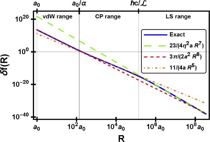
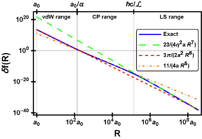
In order to illustrate the analytic considerations in Secs. III, IV and V, we numerically study the model integrals

$$I\left(a,\eta,R\right)\equiv\int_{0}^{\infty}\mathrm{d}x\,\frac{a}{\left(a-\mathrm{i}\epsilon\right)^{2}+x^{2}}\,\frac{\left(-\eta\right)}{\left(-\eta-\mathrm{i}\epsilon\right)^{2}+x^{2}}\\ \times\mathrm{e}^{-2Rx}\,\frac{x^{4}}{R^{2}}\left[1+\frac{2}{Rx}+\frac{5}{\left(Rx\right)^{2}}+\frac{6}{\left(Rx\right)^{3}}+\frac{3}{\left(Rx\right)^{4}}\right]\,,$$ (97)

which models the plain Casimir-Polder interaction as well as wave function-type corrections thereto; and

$$J\left(a,\eta,R\right)\equiv\int_{0}^{\infty}\mathrm{d}x\,\frac{a}{\left(a-\mathrm{i}\epsilon\right)^{2}+x^{2}}\\ \times\frac{\partial}{\partial\eta}\frac{\left(-\eta\right)}{\left(-\eta-\mathrm{i}\epsilon\right)^{2}+x^{2}}\\ \times\mathrm{e}^{-2Rx}\,\frac{x^{4}}{R^{2}}\left[1+\frac{2}{Rx}+\frac{5}{\left(Rx\right)^{2}}+\frac{6}{\left(Rx\right)^{3}}+\frac{3}{\left(Rx\right)^{4}}\right]$$ (98)

which models energy-type corrections to the Casimir-Polder interaction. Our choices for the numerical values of the parameters are

$\displaystyle\eta=$  $\displaystyle\;10^{-3}\;,$ (99a)
$\displaystyle a=$ $\displaystyle 1\;,$ (99b)
$\displaystyle\epsilon=$ $\displaystyle 10^{-6}\;\,.$ (99c)

These values are adapted to the investigation of the quasi-degenerate contributions to the interatomic interaction, $a$ playing the role of the energy of a transition between quantum levels with different principal quantum numbers, while $\eta$ corresponds to the energy of a transition between quasi-degenerate neighbors. These parameters and arguments are dimensionless. The transition from the $1/R^{6}$ short-range asymptotics to the $1/R^{7}$ long-range limit is clearly displayed in Fig. 1, while the intermediate $1/R^{5}$ regime for $J$ is discernible in Fig. 2.

Appendix B Details on Dirac-$\maybebm{\delta}$ corrections to the van der Waals interaction

Here we present some details on how the numerical results (78) and (79) were obtained. We recall that for the $2S$ $1S$ system, $\delta D_{6}$ is given by

$$\delta D_{6}(2S;1S)=\frac{3}{\pi}\frac{\hbar}{(4\pi\epsilon_{0})^{2}}\,\int\limits_{0}^{\infty}{\mathrm{d}}\omega\,\left[\delta_{2S}\alpha_{1S\left(2S\right)}({\mathrm{i}}\omega)\right.\\ \times\left.\alpha_{2S\left(1S\right)}({\mathrm{i}}\omega)+\alpha_{1S\left(2S\right)}({\mathrm{i}}\omega)\,\delta_{2S}\alpha_{2S\left(1S\right)}({\mathrm{i}}\omega)\right]\,,$$ (100)

where the corrected polarizabilities read

$$\delta_{2S}\alpha_{1S\left(2S\right)}(\omega)=\\ \frac{e^{2}}{3}\sum_{\pm}\left<1S\right|\vec{r}\frac{1}{\left(H-E_{\overline{1S2S}}-\mathrm{i}\epsilon\pm\hbar\omega\right)^{2}}\vec{r}\left|1S\right>\\ \times\frac{1}{2}\left<2S\right|\delta V\left|2S\right>\equiv\delta_{2S}\alpha_{1S\left(2S\right)}^{\left(E\right)}(\omega),$$ (101a)
because we perturb only the $2S$ energy, and
$$\delta_{2S}\alpha_{2S\left(1S\right)}(\omega)=\\ \frac{e^{2}}{3}\sum_{\pm}\left<2S\right|\vec{r}\frac{1}{\left(H-E_{\overline{1S2S}}-\mathrm{i}\epsilon\pm\hbar\omega\right)^{2}}\vec{r}\left|2S\right>\\ \times\frac{1}{2}\left<2S\right|\delta V\left|2S\right>\\ +\frac{2e^{2}}{3}\sum_{\pm}\left<2S\right|\vec{r}\,\frac{1}{H-E_{\overline{1S2S}}-\mathrm{i}\epsilon\pm\hbar\omega}\,\vec{r}\left|\delta 2S\right>\\ =\delta_{2S}\alpha_{2S\left(1S\right)}^{\left(E\right)}(\omega)+\delta_{2S}\alpha_{2S\left(1S\right)}^{\left(\psi\right)}(\omega).$$ (101b)

Here the $\left(E\right)$ superscript refers to the contribution from the energy correction and the $\left(\psi\right)$ superscript refers to the contribution from the wave function correction. It can be checked that the two summands in

$$\delta D_{6}^{\left(E\right)}(2S;1S)=\frac{3}{\pi}\frac{\hbar}{(4\pi\epsilon_{0})^{2}}\,\int\limits_{0}^{\infty}{\rm d}\omega\left[\delta_{2S}\alpha_{1S\left(2S\right)}^{\left(E\right)}({\mathrm{i}}\omega)\right.\\ \times\alpha_{2S\left(1S\right)}({\mathrm{i}}\omega)\left.+\alpha_{1S\left(2S\right)}({\mathrm{i}}\omega)\,\delta_{2S}\alpha_{2S\left(1S\right)}^{\left(E\right)}({\mathrm{i}}\omega)\right]$$ (102)

contribute equally. This can be traced back to the integral identity (23). The easiest way to compute the energy correction to a polarizability is to notice that

$\displaystyle\left<nS\right|\vec{r}\,\frac{1}{\left(H-E-\mathrm{i}\epsilon+\hbar\omega\right)^{2}}\,\vec{r}\left|mS\right>$
$\displaystyle=-\frac{1}{\hbar}\frac{\partial}{\partial\omega}\left<nS\right|\vec{r}\,\frac{1}{H-E-\mathrm{i}\epsilon+\hbar\omega}\,\vec{r}\left|mS\right>\,,$ (103)

which is just the $\omega$-derivative of a typical $P$ matrix element. To see that the summands in the integrand on the right-hand side of (102) contribute equally, however, one rather notices that

$\displaystyle\left<nS\right|\vec{r}\,\frac{1}{\left(H-E-\mathrm{i}\epsilon+\hbar\omega\right)^{2}}\,\vec{r}\left|mS\right>$
$\displaystyle=\frac{\partial}{\partial E}\left<nS\right|\vec{r}\,\frac{1}{H-E-\mathrm{i}\epsilon+\hbar\omega}\,\vec{r}\left|mS\right>\,,$ (104)

and the equality follows from (23). In the end, we obtain

$\displaystyle\delta D_{6}^{\left(E\right)}(2S;1S)=$  $\displaystyle\;49.733\,193\,536\,\alpha^{2}\,a_{0}^{6}\,E_{h}\,.$ (105)

It is considerably harder to compute the contribution to the van der Waals coefficient from the wave function correction

$$\delta D_{6}^{\left(\psi\right)}(2S;1S)=\frac{3\hbar}{\pi(4\pi\epsilon_{0})^{2}}\\ \times\int\limits_{0}^{\infty}{\mathrm{d}}\omega\,\alpha_{1S\left(2S\right)}({\mathrm{i}}\omega)\delta_{2S}\alpha_{2S\left(1S\right)}^{\left(\psi\right)}({\mathrm{i}}\omega).$$ (106)

The first step is to obtain the correction (73) to the $2S$ wave function, from which we deduce

$$\delta P_{2S}^{\left(\psi\right)}\left(\omega\right)=\frac{e^{2}a_{0}^{2}}{m\,c^{2}}\left(-\frac{8}{9}\,\frac{\tau^{2}Q(\tau)}{\left(1-\tau\right)^{7}\,\left(1+\tau\right)^{8}}\right.\\ +\frac{4\,096\,\tau^{9}\,(-2+\tau+7\tau^{2})}{3\,(\tau-1)^{6}\,(1+\tau)^{5}}\,\ln\left(\frac{2\tau}{1+\tau}\right)\\ +\frac{512\tau^{7}\,(1+\tau^{2})}{(1-\tau)^{5}\,(1+\tau)^{5}}{}_{2}F_{1}\left(1,-2\tau;1-2\tau;-\frac{1-\tau}{1+\tau}\right)\\ -\frac{512\tau^{7}\,R(\tau)}{9\,(1-\tau)^{7}\,(1+\tau)^{7}}{}_{2}F_{1}\left(1,-2\tau;1-2\tau;\left(\frac{1-\tau}{1+\tau}\right)^{2}\right)\\ +\frac{32\,768}{3}\frac{\tau^{10}\left(-1+4\tau^{2}\right)}{\left(-1+\tau\right)^{2}\left(1+\tau\right)^{10}}\\ \left.\times\sum_{k=0}^{\infty}\left(\frac{-1+\tau}{1+\tau}\right)^{k}\frac{\partial_{2}\,{}_{2}F_{1}\left(-k,4;4;\frac{2}{1+\tau}\right)}{\left(2+k-2\tau\right)}\right)\,,$$ (107)

where

$$Q(\tau)=-123-123\tau+801\tau^{2}+801\tau^{3}-2\,124\tau^{4}\\ -1\,932\tau^{5}+4\,002\tau^{6}+11\,234\tau^{7}+3\,661\tau^{8}-20\,979\tau^{9}\\ +2\,285\tau^{10}+9\,645\tau^{11}+26\,314\tau^{12}+3\,402\tau^{13}$$ (108)

and

$$R(\tau)=-3+113\,\tau^{2}-193\,\tau^{4}+371\tau^{6}\\ +96\tau^{2}\,(1-\tau^{2})\,(1-4\tau^{2})\,\ln\left(\frac{2\tau}{1+\tau}\right)\,.$$ (109)

Furthermore,

$$\tau=\left(1+\frac{8\hbar\omega}{\alpha^{2}mc^{2}}\right)^{-1/2}.$$ (110)

We can then easily deduce $\delta_{2S}\alpha_{2S\left(1S\right)}^{\left(\psi\right)}\left(\omega\right)$ from (107) via

$$\delta_{2S}\alpha_{2S\left(1S\right)}^{\left(\psi\right)}(\omega)=\delta_{2S}P_{2S\left(1S\right)}^{\left(\psi\right)}(\omega)+\delta_{2S}P_{2S\left(1S\right)}^{\left(\psi\right)}(-\omega)$$ (111)

where $\delta_{2S}P_{2S\left(1S\right)}^{\left(\psi\right)}\left(\omega\right)$ has the same expression as (107), with $\tau$ replaced by

$$t_{\mathrm{eff}}=\left(1+\frac{16\hbar\omega}{5\alpha^{2}mc^{2}}\right)^{-1/2}.$$ (112)

From all of this we obtain

$\displaystyle\delta D_{6}^{\left(\psi\right)}(2S;1S)=$  $\displaystyle\;318.181\,412\,174\,\alpha^{2}\,a_{0}^{6}\,E_{h}\,.$ (113)

We now recall that for the $2S$ $1S$ system, $\delta M_{6}$ is given by

$$\delta M_{6}(2S;1S)=\frac{3}{\pi}\frac{\hbar}{(4\pi\epsilon_{0})^{2}}\,\int\limits_{0}^{\infty}{\rm d}\omega\,\delta_{2S}\alpha_{\overline{1S2S}}({\mathrm{i}}\omega)\,\alpha_{\overline{1S2S}}({\mathrm{i}}\omega)$$ (114)

where the corrected mixed polarizability reads

$\displaystyle\delta_{2S}\alpha_{\overline{1S2S}}(\omega)$ $\displaystyle=\sum_{\pm}\left<1S\right|\vec{r}\frac{1}{\left(H-E_{\overline{1S2S}}-\mathrm{i}\epsilon\pm\hbar\omega\right)^{2}}\vec{r}\left|2S\right>$
$\displaystyle\times\frac{e^{2}}{3}\frac{1}{2}\left<2S\right|\delta V\left|2S\right>$
$\displaystyle+\frac{e^{2}}{3}\sum_{\pm}\left<1S\right|\vec{r}\frac{1}{H-E_{\overline{1S2S}}-\mathrm{i}\epsilon\pm\hbar\omega}\vec{r}\left|\delta 2S\right>$
$\displaystyle=\delta_{2S}\alpha_{\overline{1S2S}}^{\left(E\right)}(\omega)+\delta_{2S}\alpha_{\overline{1S2S}}^{\left(\psi\right)}(\omega)\,.$ (115)

Here again, the $\left(E\right)$ subscript refers to the contribution from the energy correction and the $\left(\psi\right)$ subscript refers to the contribution from the wave function correction. We again compute

$$\delta M_{6}^{\left(E\right)}(2S;1S)=\frac{6}{\pi}\frac{\hbar}{(4\pi\epsilon_{0})^{2}}\\ \times\int\limits_{0}^{\infty}{\rm d}\omega\,\delta_{2S}\alpha_{\overline{1S2S}}^{\left(E\right)}({\mathrm{i}}\omega)\,\alpha_{\overline{1S2S}}({\mathrm{i}}\omega)$$ (116)

by using (B). For that we need

$$P_{\overline{1S2S}}\left(\omega\right)=\frac{e^{2}a_{0}^{2}}{E_{h}}\frac{512\sqrt{2}\,t_{\mathrm{eff}}^{2}}{729\left(-1+t_{\mathrm{eff}}^{2}\right)^{2}\,\left(-4+t_{\mathrm{eff}}^{2}\right)^{3}}\\ \left[128-272t_{\mathrm{eff}}^{2}+120t_{\mathrm{eff}}^{4}+253t_{\mathrm{eff}}^{6}+972t_{\mathrm{eff}}^{7}+419t_{\mathrm{eff}}^{8}\right.\\ \left.-1944t_{\mathrm{eff}}^{7}\,{}_{2}F_{1}\left(1,-t_{\mathrm{eff}};1-t_{\mathrm{eff}};\frac{1-t_{\mathrm{eff}}}{1+t_{\mathrm{eff}}}\frac{2-t_{\mathrm{eff}}}{2+t_{\mathrm{eff}}}\right)\right]$$ (117)

with $t_{\mathrm{eff}}$ given by (112). In the end, we obtain

$\displaystyle\delta M_{6}^{\left(E\right)}(2S;1S)=$  $\displaystyle\;12.556\,663\,547\,\alpha^{2}\,a_{0}^{6}\,E_{h}\,.$ (118)

Finally, we calculate the wave-function contribution to the mixing coefficient for the Dirac-$\delta$ correction,

$$\delta M_{6}^{\left(\psi\right)}(2S;1S)=\frac{6}{\pi}\frac{\hbar}{(4\pi\epsilon_{0})^{2}}\\ \times\int\limits_{0}^{\infty}{\rm d}\omega\,\delta_{2S}\,\alpha_{\overline{1S2S}}^{\left(\psi\right)}({\mathrm{i}}\omega)\,\alpha_{\overline{1S2S}}({\mathrm{i}}\omega)\,.$$ (119)

From (73), we deduce

$$\delta P_{1S\underline{2S}}^{\left(\psi\right)}\left(\omega\right)=\frac{e^{2}a_{0}^{2}}{m\,c^{2}}\,\left(-\frac{128\sqrt{2}\tau^{2}\,S(\tau)}{2187\,\left(1-\tau^{2}\right)^{4}\,\left(1-4\tau^{2}\right)^{3}}\right.\\ -\frac{2\,048\,\sqrt{2}\,\tau^{2}\,T(\tau)}{729\,(1-\tau)^{3}\,(1+\tau)^{2}\,(1-4\tau^{2})^{2}}\,\ln\left(\frac{2\tau}{1+\tau}\right)\\ -\frac{2\,048\,\sqrt{2}\,\tau^{2}\,(1+2\tau^{2})\,U(\tau)}{729\,(1-\tau^{2})^{2}\,(1-4\tau^{2})^{3}}\,\ln\left(\frac{3\tau}{1+\tau}\right)\\ +\frac{1\,024\,\sqrt{2}\,\tau^{7}\,(1+\tau^{2})}{(1-\tau^{2})^{2}\,(1-4\tau^{2})^{3}}\,{}_{2}F_{1}\left(1,-2\tau;1-2\tau;-\frac{1-2\tau}{1+2\tau}\right)\\ +\frac{1\,024\,\sqrt{2}\,\tau^{7}\,R(\tau)}{9(1-\tau^{2})^{4}\,(1-4\tau^{2})^{3}}\\ \times{}_{2}F_{1}\left(1,-2\tau;1-2\tau;-\frac{1-\tau}{1+\tau}\,\frac{1-2\tau}{1+2\tau}\right)\\ +\frac{65\,536\sqrt{2}}{3}\,\frac{\tau^{10}}{\left(-1+\tau\right)\left(1+\tau\right)^{5}\left(1+2\tau\right)^{4}}\\ \left.\times\sum_{k=0}^{\infty}\left(-\frac{1-2\tau}{1+2\tau}\right)^{k}\frac{\partial_{2}\,{}_{2}F_{1}\left(-k,4;4;\frac{2}{1+\tau}\right)}{\left(2+k-2\tau\right)}\right)\,,$$ (120)

with $\tau$ given by (110), and $R(\tau)$ is defined in Eq. (109). The function $S(\tau)$ is given as follows,

$$S(\tau)=-157+2\,436\tau^{2}-13\,326\tau^{4}+5\,832\tau^{5}+58\,868\tau^{6}\\ +225\,504\tau^{7}-283\,245\tau^{8}+99\,144\tau^{9}\\ -431\,184\tau^{10}+695\,952\tau^{11}+200\,048\tau^{12}\,,$$ (121)

while $T(\tau)$ reads as

$$T(\tau)=2-2\tau-15\tau^{2}+15\tau^{3}+15\tau^{4}\\ -15\tau^{5}+268\tau^{6}+1\,676\tau^{7}\,,$$ (122)

and $U(\tau)$ is

$$U(\tau)=-2+27\tau^{2}-129\tau^{4}+50\tau^{6}\,.$$ (123)

We can then easily deduce $\delta_{2S}\alpha_{\overline{1S2S}}^{\left(\psi\right)}\left(\omega\right)$ from (120) via

$$\delta_{2S}\alpha_{\overline{1S2S}}^{\left(\psi\right)}(\omega)=\delta_{2S}P_{\overline{1S2S}}^{\left(\psi\right)}(\omega)+\delta_{2S}P_{\overline{1S2S}}^{\left(\psi\right)}(-\omega)$$ (124)

where again $\delta_{2S}P_{\overline{1S2S}}^{\left(\psi\right)}\left(\omega\right)$ has the same expression as (120), with $\tau$ replaced by $t_{\mathrm{eff}}$ [see (112)]. From all of this we obtain

$\displaystyle\delta M_{6}^{\left(\psi\right)}(2S;1S)=$ $\displaystyle\;-70.652\,014\,640\,\alpha^{2}\,a_{0}^{6}\,E_{h}\,.$ (125)

References

  • Jentschura and Yerokhin (2006) U. D. Jentschura and V. A. Yerokhin, “Quantum electrodynamic corrections to the hyperfine structure of excited $S$ states,” Phys. Rev. A 73, 062503 (2006).
  • Bethe (1947) H. A. Bethe, “The Electromagnetic Shift of Energy Levels,” Phys. Rev. 72, 339–341 (1947).
  • Chibisov (1972) M. I. Chibisov, “Dispersion Interaction of Neutral Atoms,” Opt. Spectrosc. 32, 1–3 (1972).
  • Deal and Young (1973) W. J. Deal and R. H. Young, “Long–Range Dispersion Interactions Involving Excited Atoms; the H(1s)—H(2s) Interaction,” Int. J. Quantum Chem. 7, 877–892 (1973).
  • Tang and Chan (1986) A. Z. Tang and F. T. Chan, “Dynamic Multipole polarizability of atomic hydrogen,” Phys. Rev. A 33, 3671–3678 (1986).
  • Kolachevsky et al. (2004) N. Kolachevsky, M. Fischer, S. G. Karshenboim,  and T. W. Hänsch, “High-Precision Optical Measurement of the $2S$ Hyperfine Interval in Atomic Hydrogen,” Phys. Rev. Lett. 92, 033003 (2004).
  • Kolachevsky et al. (2009) N. Kolachevsky, A. Matveev, J. Alnis, C. G. Parthey, S. G. Karshenboim,  and T. W. Hänsch, “Measurement of the $2S$ Hyperfine Interval in Atomic Hydrogen,” Phys. Rev. Lett. 102, 213002 (2009).
  • Dalgarno and Davidson (1966) A. Dalgarno and W. D. Davidson, “The Calculation of Van Der Waals Interactions,” Adv. At. Mol. Opt. Phys. 2, 1–32 (1966).
  • Dalgarno (1967) A. Dalgarno, “New Methods for Calculating Long–Range Intermolecular Forces,” Adv. Chem. Phys. 12, 143–166 (1967).
  • Ray et al. (1968a) S. Ray, J. D. Lyons,  and T. P. Das, “Hyperfine Pressure Shift and van der Waals Interactions. I. Hydrogen–Helium System,” Phys. Rev. 174, 104–112 (1968a), erratum Phys. Rev. 181, 465 (1969)].
  • Ray et al. (1968b) S. Ray, J. D. Lyons,  and T. P. Das, “Hyperfine Pressure Shift and van der Waals Interactions. II. Nitrogen–Helium System,” Phys. Rev. 174, 112–118 (1968b), erratum Phys. Rev. 181, 465 (1969)].
  • Rao and Das (1969) B. K. Rao and T. P. Das, “Hyperfine Pressure Shift and van der Waals Interactions. III. Temperature Dependence,” Phys. Rev. 185, 95–97 (1969).
  • Rao and Das (1970) B. K. Rao and T. P. Das, “Hyperfine Pressure Shift and van der Waals Interactions. IV. Hydrogen–Rare–Gas Systems,” Phys. Rev. A 2, 1411–1421 (1970).
  • Dalgarno et al. (1968) A. Dalgarno, G. W. F. Drake,  and G. A. Victor, “Nonadiabatic Long–Range Forces,” Phys. Rev. 176, 194–197 (1968).
  • Dutta et al. (1970) C. M. Dutta, N. C. Dutta,  and T. P. Das, “Many–Body Approach to the Hyperfine Pressure Shift in Optical–Pumping Experiments,” Phys. Rev. A 2, 30–37 (1970).
  • Yan et al. (1996) Z. C. Yan, J. F. Babb, A. Dalgarno,  and G. W. F. Drake, “Variational calculations of dispersion coefficients for interactions among h, he, and li atoms,” Phys. Rev. A 54, 2824–2833 (1996).
  • Yan et al. (1997) Z. C. Yan, A. Dalgarno,  and J. F. Babb, “Long-range interactions of lithium atoms,” Phys. Rev. A 55, 2882–2887 (1997).
  • Jamieson et al. (1995) M. J. Jamieson, G. W. F. Drake,  and A. Dalgarno, “Retarded dipole-dipole dispersion interaction potential for helium,” Phys. Rev. A 51, 3358–3361 (1995).
  • Chen and Chung (1996) M. K. Chen and K. T. Chung, “Retardation long-range potentials between two helium atoms,” Phys. Rev. A 53, 1439–1446 (1996).
  • Marinescu et al. (1994) M. Marinescu, H. R. Sadeghpour,  and A. Dalgarno, “Dispersion coefficients for alkali-metal dimers,” Phys. Rev. A 49, 982–988 (1994).
  • Marinescu and Dalgarno (1995) M. Marinescu and A. Dalgarno, “Dispersion forces and long-range electronic transition dipole moments of alkali-metal dimer excited states,” Phys. Rev. A 52, 311–328 (1995).
  • Pachucki (2005) K. Pachucki, “Relativistic corrections to the long-range interaction between closed-shell atoms,” Phys. Rev. A 72, 062706 (2005).
  • Berestetskii et al. (1982) V. B. Berestetskii, E. M. Lifshitz,  and L. P. Pitaevskii, Quantum Electrodynamics, Volume 4 of the Course on Theoretical Physics, 2nd ed. (Pergamon Press, Oxford, UK, 1982).
  • Karshenboim and Ivanov (1997) S. G. Karshenboim and V. G. Ivanov, “Radiative Corrections to the $2E1$ Decay Rate of the $2s$-State in Hydrogen-Like Atoms,” Opt. Spectrosc. 83, 1–5 (1997).
  • Jentschura (2004) U. D. Jentschura, “Self–Energy Correction to the Two–Photon Decay Width in Hydrogenlike Atoms,” Phys. Rev. A 69, 052118 (2004).
  • Itzykson and Zuber (1980) C. Itzykson and J. B. Zuber, Quantum Field Theory (McGraw-Hill, New York, 1980).
  • Mohr et al. (2012) P. J. Mohr, B. N. Taylor,  and D. B. Newell, “CODATA Recommended Values of the Fundamental Physical Constants: 2010,” Rev. Mod. Phys. 84, 1527–1605 (2012).
  • Power and Thirunamachandran (1995) E. A. Power and T. Thirunamachandran, “Dispersion forces between molecules with one or both molecules excited,” Phys. Rev. A 51, 3660–3666 (1995).
  • Safari and Karimpour (2015) H. Safari and M. R. Karimpour, “Body-Assisted van der Waals Interaction between Excited Atoms,” Phys. Rev. Lett. 114, 013201 (2015).
  • Donaire et al. (2015) M. Donaire, R. GuĂŠrout,  and A. Lambrecht, “Quasiresonant van der Waals Interaction between Nonidentical Atoms,” Phys. Rev. Lett. 115, 033201 (2015).
  • Jentschura and Debierre (2016) U. D. Jentschura and V. Debierre, Long–Range Tails in van der Waals Interactions of Excited–State and Ground–State Atoms, in preparation (2016).
  • Bethe and Salpeter (1957) H. A. Bethe and E. E. Salpeter, Quantum Mechanics of One- and Two-Electron Atoms (Springer, Berlin, 1957).
  • Gavrila and Costescu (1970) M. Gavrila and A. Costescu, “Retardation in the Elastic Scattering of Photons by Atomic Hydrogen,” Phys. Rev. A 2, 1752–1758 (1970).
  • Pachucki (1993) K. Pachucki, “Higher-Order Binding Corrections to the Lamb Shift,” Ann. Phys. (N.Y.) 226, 1–87 (1993).
  • Jentschura and Pachucki (1996) U. Jentschura and K. Pachucki, “Higher-order binding corrections to the Lamb shift of $2{P}$ states,” Phys. Rev. A 54, 1853–1861 (1996).
  • Swainson and Drake (1991) R. A. Swainson and G. W. F. Drake, “A unified treatment of the non-relativistic and relativistic hydrogen atom II: the Green functions,” J. Phys. A 24, 95–120 (1991).
  • Bateman (1953) H. Bateman, Higher Transcendental Functions, Vol. 1 (McGraw-Hill, New York, 1953).
  • Adhikari et al. (2016) C. M. Adhikari, A. Kawasaki,  and U. D. Jentschura, “Magic Wavelength for the hydrogen $1S$ $2S$ transition: Contribution of the continuum and the reduced-mass correction,” Phys. Rev. A 94, 032510 (2016).
  • Salomonson and Öster (1989) S. Salomonson and P. Öster, “Solution of the pair equation using a finite discrete spectrum,” Phys. Rev. A 40, 5559–5567 (1989).
  • Kołos (1967) W. Kołos, “Long-range interaction between $1S$ and $2S$ or $2p$ hydrogen atoms,” Int. J. Quantum Chem. 1, 169–186 (1967).
  • Casimir and Polder (1948) H. B. G. Casimir and D. Polder, “The Influence of Radiation on the London-van-der-Waals Forces,” Phys. Rev. 73, 360–372 (1948).
  • Jentschura (2015) U. D. Jentschura, “Long-range atom-wall interactions and mixing terms: Metastable hydrogen,” Phys. Rev. A 91, 010502(R) (2015).
  • Jentschura (2003) U. D. Jentschura, “Corrections to Bethe Logarithms induced by Local Potentials,” J. Phys. A 36, L229 (2003).
  • Essen et al. (1971) L. Essen, R. W. Donaldson, M. J. Bangham,  and E. G. Hope, “Frequency of the Hydrogen Maser,” Nature (London) 229, 110 (1971).
  • Essen et al. (1973) L. Essen, R. W. Donaldson, E. G. Hope,  and M. J. Bangham, “Hydrogen Maser Work at the National Physical Laboratory,” Metrologia 9, 128 (1973).
  • Petit et al. (1980) P. Petit, M. Descaintfuscien,  and C. Audoin, “Temperature Dependence of the Hydrogen Maser Wall Shift in the Temperature Range 295–395K,” Metrologia 16, 7–14 (1980).
  • Varshalovich et al. (1988) D. A. Varshalovich, A. N. Moskalev,  and V. K. Khersonskii, Quantum Theory of Angular Momentum (World Scientific, Singapore, 1988).
  • Parthey et al. (2011) C. G. Parthey, A. Matveev, J. Alnis, B. Bernhardt, A. Beyer, R. Holzwarth, A. Maistrou, R. Pohl, K. Predehl, T. Udem, T. Wilken, N. Kolachevsky, M. Abgrall, D. Rovera, C. Salomon, P. Laurent,  and T. W. Hänsch, “Improved Measurement of the Hydrogen 1S–2S Transition Frequency,” Phys. Rev. Lett. 107, 203001 (2011).
  • Fee et al. (1993) M. S. Fee, A. P. Mills, S. Chu, E. D. Shaw, K. Danzmann, R. J. Chichester,  and D. M. Zuckerman, “Measurement of the positronium $1{}^{3}S_{1}$ $2{}^{3}S_{1}$ interval by continuous-wave two-photon excitation,” Phys. Rev. Lett. 70, 1397–1400 (1993).