$B_{c}\to(J/\Psi,\,\eta_{c})\tau\nu$ semileptonic decays within Standard model and beyond.

Abstract

Deviations from the standard model prediction have been observed not only in $b\to c$ charged current interactions but also in $b\to s$ flavor changing neutral current interactions. In particular, the deviation observed in the measured ratio of branching fractions $R_{D}=\mathcal{B}(B\to D\tau\nu)/\mathcal{B}(B\to D\,l\,\nu)$ and $R_{D^{\ast}}=\mathcal{B}(B\to D^{\ast}\tau\nu)/\mathcal{B}(B\to D^{\ast}\,l\,\nu)$, where $l=(e,\,\mu)$, is more pronounced and the combined excess currently stands at $3.9\sigma$ level. If it persists and confirmed by future experiments, it would be a definite hint of new physics. In this context, we consider $B_{c}\to\eta_{c}\,l\,\nu$ and $B_{c}\to J/\Psi\,l\,\nu$ decays mediated via $b\to c\,l\,\nu$ charged current interactions and employ the most general effective Lagrangian in the presence of new physics to give prediction on various observables such as ratio of branching ratio, tau polarization fraction, and forward backward asymmetry for these decay modes.

I Introduction

Although, no direct evidence of new physics has been reported so far, there still exists some discrepancies with the standard model (SM) prediction. In particular, deviations from the SM expectation in both charged current $b\to c\tau\nu$ transitions as well as neutral current $b\to s\,l\bar{l}$ transitions have been observed in various measurements. The decays $B\to(D,\,D^{\ast})\tau\nu$ and the lepton flavor universality ratios $R_{D}$ and $R_{D^{\ast}}$ have been studied by BABAR Lees:2012xj ; Lees:2013uzd , BELLE Huschle:2015rga ; Sato:2016svk ; Abdesselam:2016xqt , and LHCb Aaij:2015yra experiments. Various measurements of $R_{D}$ and $R_{D^{\ast}}$ are collected in Table. 1.

Experiments	$R_{D^{\ast}}$	$R_{D}$
BABAR	$0.332\pm 0.024\pm 0.018$	$0.440\pm 0.058\pm 0.042$
BELLE	$0.293\pm 0.038\pm 0.015$	$0.375\pm 0.064\pm 0.026$
BELLE	$0.302\pm 0.030\pm 0.011$
LHCb	$0.336\pm 0.027\pm 0.030$
BELLE	$0.276\pm 0.034^{+0.029}_{-0.026}$
AVERAGE	$0.310\pm 0.015\pm 0.008$	$0.403\pm 0.040\pm 0.024$

Table 1: Current status of $R_{D}$ and $R_{D^{\ast}}$ hfag .

The first unquenched lattice determination of the ratio of branching ratio $R_{D}=0.299\pm 0.011$ Lattice:2015rga was reported by FNAL/MILC collaboration which is in excellent agreement with the the value of $R_{D}=0.300\pm 0.008$ Na:2015kha reported by HPQCD collaboration. In Ref. Bigi:2016mdz , the authors obtain $R_{D}=0.299\pm 0.003$ by combining the two lattice calculations, with the experimental form factor of the $B\to D\,l\,\nu$ from BABAR and BELLE. The result is compatible with the results above, but more accurate. The FLAG working group combine the two lattice calculations and report the value of $R_{D}$ to be $0.300\pm 0.008$ Aoki:2016frl . The SM prediction for $R_{D^{\ast}}$ is $0.252\pm 0.003$ Fajfer:2012vx . At present, the deviation of the measured values of $R_{D}$ and $R_{D^{\ast}}$ from the SM expectation exceeded by $2.2\sigma$ and $3.4\sigma$ respectively hfag . Considering the $R_{D}$-$R_{D^{\ast}}$ correlation, the difference with the SM predictions currently stands at about $3.9\sigma$ hfag . For theoretical implications of these anomalies, we refer to Refs. Fajfer:2012vx ; Fajfer1 ; Hou ; Akeroyd ; tanaka ; Nierste ; miki ; Wahab ; Deschamps ; Blankenburg ; Ambrosio ; Buras ; Pich ; Jung ; Crivellin ; datta ; datta1 ; datta2 ; datta3 ; datta4 ; fazio ; Crivellin1 ; Celis ; He ; dutta ; Tanaka:2016ijq ; Deshpand:2016cpw ; Li:2016vvp ; Du:2015tda ; Bernlochner:2015mya ; Soffer:2014kxa ; Bordone:2016tex ; Bardhan:2016uhr ; Alok:2016qyh ; Ivanov:2015tru ; Ivanov:2016qtw ; Boucenna:2016wpr ; Boucenna:2016qad ; Nandi:2016wlp ; Dutta:2016eml ; Alonso:2016oyd ; Becirevic:2016yqi ; Celis:2016azn and references therein. Very recently, the first measurement of the tau polarization fraction $P_{\tau}^{D^{\ast}}=-0.44\pm 0.47^{+0.20}_{-0.17}$ in the decay $B\to D^{\ast}\tau\nu$ was reported by BELLE Abdesselam:2016xqt .

$B_{c}$ meson, a pseudoscalar ground state composed of two heavy quarks $b$ and $c$, first observed by CDF collaboration in $p\bar{p}$ collisions Abe:1998fb , has a promising prospect on the hadron colliders as around $5\times 10^{10}$ $B_{c}$ events per year are expected at LHC experiments Gouz:2002kk ; Altarelli:2008xy . Being composed of two heavy quarks, $B_{c}$ meson has the unique ability to decay via both $b$ and $c$ quark. Although the $b$ decays are cabbibo suppressed, the charm quark decays, however, are cabbibo favored decays as the CKM matrix element $V_{cs}=1$ is much larger than $V_{cb}=0.04$. The estimates of the $B_{c}$ total decay width indicate that the $c$ quark transitions provide the dominant contribution while the $b$ quark transitions and weak annihilation contribute less. The $c$ quark decays provide around $70\%$ to the total decay width of $B_{c}$ meson Gouz:2002kk . Although an indirect constraint can be imposed on various new physics (NP) from the experimentally measured total decay width of $B_{c}$ meson, however, measurement of various taunic decays of $B_{c}$ meson in future will give direct access to the beyond the SM physics. The mean lifetime of $B_{c}$ meson $\tau_{B_{c}}=0.52^{+0.18}_{-0.12}\,{\rm ps}$ in the SM, calculated using operator product expansion and non relativistic QCD Bigi:1995fs ; Beneke:1996xe ; Chang:2000ac , is consistant with the measured mean lifetime $\tau_{B_{c}}=0.507(8){\rm ps}$ pdg . One can infer from this calculation that no more than $5\%$ of the total decay width of $B_{c}$ meson can be explained by the semi(taunic) decays of $B_{c}$ meson. This was confirmed by various other SM caculations as well Gershtein:1994jw ; Kiselev:2000pp . The constraint, however, can be relaxed upto around $30\%$ depending on the value of the total decay width of $B_{c}$ meson that is used as input for the SM calculation of various partonic transitions.

The $B_{c}$ meson and its decays have been widely studied in the literature Dhir:2008hh ; Hernandez:2006gt ; Ivanov:2000aj ; Ivanov:2005fd ; Ivanov:2006ni ; Ebert:2002pp ; Ebert:2003cn ; Ebert:2003wc ; Du:1988ws ; Chang:1992pt ; Liu:1997hr ; AbdElHady:1999xh ; Colangelo:1999zn ; Sun:2008wa ; Wang:2008xt ; Qiao:2012vt ; Xiao:2011zz ; Liu:2009qa ; Cheng:2005um ; Sun:2008ew ; Wen-Fei:2013uea ; Pathak:2013dra ; Hsiao:2016pml . The decays $B_{c}\to(J/\Psi,\,\eta_{c})\,l\,\nu$ are mediated via $b\to c\,l\,\nu$ transitions and, in principle, NP effects might enter into these decay modes as well. The SM prediction of these decay modes are already studied by various authors Hernandez:2006gt ; Ivanov:2000aj ; Ivanov:2005fd ; Ivanov:2006ni ; Ebert:2003cn ; AbdElHady:1999xh ; Colangelo:1999zn ; Qiao:2012vt ; Wen-Fei:2013uea ; Pathak:2013dra ; Hsiao:2016pml . Earlier discussions, however, have not looked into possible NP effects in these decay modes. In this study, we wish to study systematically the effect of NP couplings on various observables such as ratio of branching ratios, forward backward asymmetry, and $\tau$ polarization fraction pertaining to $B_{c}\to(J/\Psi,\,\eta_{c})\,\tau\,\nu$ decays. To analyse the effect of NP couplings on various observables, we use the most general effective Lagrangian for the $b\to c\,l\,\nu$ decay processes in the presence of NP that is valid at the renormalization scale $\mu=m_{b}$. We use $2\sigma$ constraint coming from the measured values of the ratio of branching ratios $R_{D}$ and $R_{D^{\ast}}$ to explore various NP scenarios. Constraint coming from total decay width of $B_{c}$ meson is also discussed in details. We, however, do not use the constraint coming from the measured value of $P_{\tau}^{D^{\ast}}$ as the uncertainty associated with this observable reported by BELLE is rather large.

Our paper is organised as follows. In section II, we introduce the most general effective Lagrangian for the $b\to c\,l\,\nu$ transition decays in the presence of NP. The two body $B_{c}\to\tau\nu$ and three body $B_{c}\to(J/\Psi,\,\eta_{c})\,l\,\nu$ decay branching ratios are calculated and reported in section II. Various observables such as ratio of branching ratios, forward backward asymmetries, and the $\tau$ polarization are defined. We report our analysis in section III with a conclusion and summary in section IV.

II Effective weak Lagrangian, helicity amplitudes, and observables

II.1 Effective weak Lagrangian

We employ the effective field theory approach for the computation of various decay branching fractions in a model independent way. The most general effective weak Lagrangian at energy scale $\mu=m_{b}$ for the $b\to c\,l\,\nu$ transition decays can be expressed as Bhattacharya ; Cirigliano

$$\mathcal{L}_{\rm eff} = -\frac{4\,G_{F}}{\sqrt{2}}\,V_{cb}\,\Bigg{\{}(1+V_{L})\,\bar{l}_{L}\,\gamma_{\mu}\,\nu_{L}\,\bar{c}_{L}\,\gamma^{\mu}\,b_{L}+V_{R}\,\bar{l}_{L}\,\gamma_{\mu}\,\nu_{L}\,\bar{c}_{R}\,\gamma^{\mu}\,b_{R}+\widetilde{V}_{L}\,\bar{l}_{R}\,\gamma_{\mu}\,\nu_{R}\,\bar{c}_{L}\,\gamma^{\mu}\,b_{L}$$ (1)

$$+\widetilde{V}_{R}\,\bar{l}_{R}\,\gamma_{\mu}\,\nu_{R}\,\bar{c}_{R}\,\gamma^{\mu}\,b_{R}+S_{L}\,\bar{l}_{R}\,\nu_{L}\,\bar{c}_{R}\,b_{L}+S_{R}\,\bar{l}_{R}\,\nu_{L}\,\bar{c}_{L}\,b_{R}+\widetilde{S}_{L}\,\bar{l}_{L}\,\nu_{R}\,\bar{c}_{R}\,b_{L}+\widetilde{S}_{R}\,\bar{l}_{L}\,\nu_{R}\,\bar{c}_{L}\,b_{R}$$

$$+T_{L}\,\bar{l}_{R}\,\sigma_{\mu\nu}\,\nu_{L}\,\bar{c}_{R}\,\sigma^{\mu\nu}\,b_{L}+\widetilde{T}_{L}\,\bar{l}_{L}\,\sigma_{\mu\nu}\,\nu_{R}\,\bar{c}_{L}\,\sigma^{\mu\nu}\,b_{R}\Bigg{\}}+{\rm h.c.}\,,$$

Neglecting the tensor NP couplings and following the same notation as in Ref. dutta , the effective Lagrangian can be expressed as

$$\mathcal{L}_{\rm eff} = -\frac{G_{F}}{\sqrt{2}}\,V_{cb}\,\Bigg{\{}G_{V}\,\bar{l}\,\gamma_{\mu}\,(1-\gamma_{5})\,\nu_{l}\,\bar{c}\,\gamma^{\mu}\,b-G_{A}\,\bar{l}\,\gamma_{\mu}\,(1-\gamma_{5})\,\nu_{l}\,\bar{c}\,\gamma^{\mu}\,\gamma_{5}\,b+G_{S}\,\bar{l}\,(1-\gamma_{5})\,\nu_{l}\,\bar{c}\,b$$ (2)

$$-G_{P}\,\bar{l}\,(1-\gamma_{5})\,\nu_{l}\,\bar{c}\,\gamma_{5}\,b+\widetilde{G}_{V}\,\bar{l}\,\gamma_{\mu}\,(1+\gamma_{5})\,\nu_{l}\,\bar{c}\,\gamma^{\mu}\,b-\widetilde{G}_{A}\,\bar{l}\,\gamma_{\mu}\,(1+\gamma_{5})\,\nu_{l}\,\bar{c}\,\gamma^{\mu}\,\gamma_{5}\,b$$

$$+\widetilde{G}_{S}\,\bar{l}\,(1+\gamma_{5})\,\nu_{l}\,\bar{c}\,b-\widetilde{G}_{P}\,\bar{l}\,(1+\gamma_{5})\,\nu_{l}\,\bar{c}\,\gamma_{5}\,b\Bigg{\}}+{\rm h.c.}\,,$$

where

$$G_{V}=1+V_{L}+V_{R}\,,\qquad\qquad G_{A}=1+V_{L}-V_{R}\,,\qquad\qquad G_{S}=S_{L}+S_{R}\,,\qquad\qquad G_{P}=S_{L}-S_{R}\,$$

$$\widetilde{G}_{V}=\widetilde{V}_{L}+\widetilde{V}_{R}\,,\qquad\qquad\widetilde{G}_{A}=\widetilde{V}_{L}-\widetilde{V}_{R}\,,\qquad\qquad\widetilde{G}_{S}=\widetilde{S}_{L}+\widetilde{S}_{R}\,,\qquad\qquad\widetilde{G}_{P}=\widetilde{S}_{L}-\widetilde{S}_{R}\,.$$

Here $G_{F}$ is the Fermi coupling constant and $V_{cb}$ is the CKM matrix element. The new vector and scalar NP interactions that involve left handed neutrinos are denoted by $V_{L,\,R}$ and $S_{L,\,R}$ NP couplings. Similarly for the right handed neutrinos the NP interactions are denoted by $\widetilde{V}_{L,\,R}$ and $\widetilde{S}_{L,\,R}$ NP couplings, respectively. All these NP couplings are defined at the renormalization scale $\mu=m_{b}$. In the SM, all the NP couplings will be zero leading to $G_{V,A}=1$, $G_{S,P}=0$ and $\widetilde{G}_{V,A,S,P}=0$.

II.2 Helicity amplitudes and observables

We follow Refs. Korner ; Kadeer to calculate the various helicity amplitudes for a $B_{q}$ meson decaying to a pseudoscalar or to a vector meson along with a charged lepton and an antineutrino in the final state. Again, in order to calculate the partial decay width of $B_{q}\to l\nu$ and differential decay rate of three body $B_{q}\to(P,\,V)l\nu$ decays, we need information on various nonperturbative hadronic matrix elements which are parameterized in terms of $B_{q}$ meson decay constants and $B_{q}\to(P,\,V)$ transition form factors. We refer to Refs. dutta ; Wen-Fei:2013uea for a more detailed discussion.

In the presence of NP, the partial decay width of $B_{q}\to l\,\nu$ and differential decay width of three body $B_{q}\to(P,\,V)\,l\,\nu$ decays, where $P(V)$ stands for a pseudoscalar(vector) meson, can be expressed as dutta

$$\Gamma(B_{q}\to l\nu) = \frac{G_{F}^{2}\,|V_{cb}|^{2}}{8\,\pi}\,f_{B}^{2}\,m_{l}^{2}\,m_{B_{q}}\,\Big{(}1-\frac{m_{l}^{2}}{m_{B_{q}}^{2}}\Big{)}^{2}\,\Bigg{\{}\Big{[}G_{A}-\frac{m_{B_{q}}^{2}}{m_{l}\,(m_{b}(\mu)+m_{c}(\mu))}\,G_{P}\Big{]}^{2}$$ (3)

$$+\Big{[}\widetilde{G}_{A}-\frac{m_{B_{q}}^{2}}{m_{l}\,(m_{b}(\mu)+m_{c}(\mu))}\,\widetilde{G}_{P}\Big{]}^{2}\Bigg{\}}\,,$$

$$\frac{d\Gamma^{P}}{dq^{2}} = \frac{8\,N\,|\overrightarrow{p}_{P}|\,}{3}\Bigg{\{}\,H_{0}^{2}\,\Big{(}G_{V}^{2}+\widetilde{G}_{V}^{2}\Big{)}\,\Big{(}1+\frac{\,m_{l}^{2}}{2\,q^{2}}\Big{)}$$ (4)

$$+\frac{3\,m_{l}^{2}}{2\,q^{2}}\,\Big{[}\Big{(}H_{t}\,G_{V}+\frac{\sqrt{q^{2}}}{m_{l}}\,H_{S}\,G_{S}\Big{)}^{2}+\Big{(}H_{t}\,\widetilde{G}_{V}+\frac{\sqrt{q^{2}}}{m_{l}}\,H_{S}\,\widetilde{G}_{S}\Big{)}^{2}\Big{]}\Bigg{\}}\,$$

and

$$\frac{d\Gamma^{V}}{dq^{2}} = \frac{8\,N\,|\overrightarrow{p}_{V}|}{3}\,\Bigg{\{}\mathcal{A}_{AV}^{2}+\,\frac{m_{l}^{2}}{2\,q^{2}}\Big{[}\mathcal{A}_{AV}^{2}+3\mathcal{A}_{tP}^{2}\Big{]}+\widetilde{\mathcal{A}}_{AV}^{2}+\,\frac{m_{l}^{2}}{2\,q^{2}}\Big{[}\widetilde{\mathcal{A}}_{AV}^{2}+3\mathcal{\widetilde{A}}_{tP}^{2}\Big{]}\Bigg{\}}\,,$$ (5)

where

$$N=\frac{G_{F}^{2}\,|V_{c\,b}|^{2}\,q^{2}}{256\,\pi^{3}\,m_{B_{q}}^{2}}\,\Big{(}1-\frac{m_{l}^{2}}{q^{2}}\Big{)}^{2}\,,\qquad\qquad H_{0}=\frac{2\,m_{B_{q}}\,|\overrightarrow{p}_{P}|}{\sqrt{q^{2}}}\,F_{+}(q^{2})$$

$$H_{t}=\frac{m_{B_{q}}^{2}-m_{P}^{2}}{\sqrt{q^{2}}}\,F_{0}(q^{2})\,,\qquad\qquad H_{S}=\frac{m_{B_{q}}^{2}-m_{P}^{2}}{m_{b}(\mu)-m_{c}(\mu)}\,F_{0}(q^{2})\,,$$

$$\mathcal{A}_{AV}^{2}=\mathcal{A}_{0}^{2}\,G_{A}^{2}+\mathcal{A}_{\parallel}^{2}\,G_{A}^{2}+\mathcal{A}_{\perp}^{2}\,G_{V}^{2}\,,\qquad\qquad\widetilde{\mathcal{A}}_{AV}^{2}=\mathcal{A}_{0}^{2}\,\widetilde{G}_{A}^{2}+\mathcal{A}_{\parallel}^{2}\,\widetilde{G}_{A}^{2}+\mathcal{A}_{\perp}^{2}\,\widetilde{G}_{V}^{2}\,,$$

$$\mathcal{A}_{tP}=\mathcal{A}_{t}\,G_{A}+\frac{\sqrt{q^{2}}}{m_{l}}\,\mathcal{A}_{P}\,G_{P}\,,\qquad\qquad\mathcal{\widetilde{A}}_{tP}=\mathcal{A}_{t}\,\widetilde{G}_{A}+\frac{\sqrt{q^{2}}}{m_{l}}\,\mathcal{A}_{P}\,\widetilde{G}_{P}\,.$$ (6)

and

$$\mathcal{A}_{0}=\frac{1}{2\,m_{V}\,\sqrt{q^{2}}}\Big{[}\Big{(}\,m_{B_{q}}^{2}-m_{V}^{2}-q^{2}\Big{)}(m_{B_{q}}+m_{V})A_{1}(q^{2})\,-\,\frac{4M_{B}^{2}|\vec{p}_{V}|^{2}}{m_{B_{q}}+m_{V}}A_{2}(q^{2})\Big{]}\,,$$

$$\mathcal{A}_{\parallel}=\frac{2(m_{B_{q}}+m_{V})A_{1}(q^{2})}{\sqrt{2}}\,,\qquad\qquad\mathcal{A}_{\perp}=-\frac{4m_{B_{q}}V(q^{2})|\vec{p}_{V}|}{\sqrt{2}(m_{B_{q}}+m_{V})}\,,$$

$$\mathcal{A}_{t}=\frac{2m_{B_{q}}|\vec{p}_{V}|A_{0}(q^{2})}{\sqrt{q^{2}}}\,,\qquad\qquad\mathcal{A}_{P}=-\frac{2m_{B_{q}}|\vec{p}_{V}|A_{0}(q^{2})}{(m_{b}(\mu)+m_{c}(\mu))}\,.$$ (7)

Here $|\overrightarrow{p}_{P(V)}|=\sqrt{\lambda(m_{B_{q}}^{2},\,m_{P(V)}^{2},\,q^{2})}/2\,m_{B_{q}}$ is the three momentum vector of the outgoing meson and $\lambda(a,\,b,\,c)=a^{2}+b^{2}+c^{2}-2\,(a\,b+b\,c+c\,a)$.

We define several observables such as ratio of branching ratios and tau polarization fraction for various semileptonic $b\to c$ transition decays. Those are

$$R_{M}=\frac{\mathcal{B}(B_{q}\to M\tau\nu)}{\mathcal{B}(B_{q}\to M\,l\nu)}\,,\qquad\qquad P_{\tau}^{M}=\frac{\Gamma^{M}(+)-\Gamma^{M}(-)}{\Gamma^{M}(+)+\Gamma^{M}(-)}\,,$$ (8)

where, $l$ is either an electron or a muon and $B_{q}$ is either a $B$ meson or a $B_{c}$ meson. Similarly, $M$ refers to the outgoing pseudoscalar or vector meson. Again, $\Gamma(+)$ and $\Gamma(-)$ denote the decay widths of positive and negative helicity $\tau$ lepton, respectively. It is also worth mentioning that, for $B_{q}\to P\tau\nu$ decays, the tau polarization fraction does not depend on $V_{L,\,R}$ and $\widetilde{V}_{L,\,R}$ NP couplings if we assume that NP effect is coming from new vector interactions only. We also construct various $q^{2}$ dependent observables such as differential branching fractions DBR$(q^{2})$, the ratio of branching fractions $R(q^{2})$, and the forward-backward asymmetry parameter $A^{FB}(q^{2})$ for the $B_{c}\to(\eta_{c},\,J/\Psi)\tau\nu$ decays such that

$$DBR(q^{2})=\Big{(}\frac{d\Gamma}{dq^{2}}\Big{)}/\Gamma_{tot}\,,\qquad\qquad R(q^{2})=\frac{DBR(q^{2})\Big{(}B\to(P,\,V)\,\tau\,\nu\Big{)}}{DBR(q^{2})\Big{(}B\to(P,\,V)\,l\,\nu\Big{)}}$$

$$[A^{FB}]_{(P,\,V)}(q^{2})=\frac{\Big{(}\int_{-1}^{0}-\int_{0}^{1}\Big{)}d\cos\theta_{l}\frac{d\Gamma^{(P,\,V)}}{dq^{2}\,d\cos\theta_{l}}}{\frac{d\Gamma^{(P,\,V)}}{dq^{2}}}\,.$$ (9)

In the presence of various NP couplings, the forward backward asymmetry parameter for $B_{q}\to P\,l\,\nu$ decays can be written as

$$A^{FB}_{P}(q^{2}) = \frac{3\,m_{l}^{2}}{2\,q^{2}}\frac{H_{0}\,G_{V}\,\Big{[}\Big{(}H_{t}\,G_{V}+\frac{\sqrt{q^{2}}}{m_{l}}\,H_{S}\,G_{S}\Big{)}+\Big{(}H_{t}\,\widetilde{G}_{V}+\frac{\sqrt{q^{2}}}{m_{l}}\,H_{S}\,\widetilde{G}_{S}\Big{)}\,\Big{]}}{H_{0}^{2}\,(G_{V}^{2}+\widetilde{G}_{V}^{2})(1+\frac{m_{l}^{2}}{2\,q^{2}})+\frac{3\,m_{l}^{2}}{2\,q^{2}}\,\Big{[}\Big{(}H_{t}\,G_{V}+\frac{\sqrt{q^{2}}}{m_{l}}\,H_{S}\,G_{S}\Big{)}^{2}+\Big{(}H_{t}\,\widetilde{G}_{V}+\frac{\sqrt{q^{2}}}{m_{l}}\,H_{S}\,\widetilde{G}_{S}\Big{)}^{2}\,\Big{]}}\,.$$

Similarly, for $B_{q}\to V\,l\,\nu$ decay mode, the explicit expression for the forward backward asymmetry parameter is

$$A^{FB}_{V}(q^{2}) = \frac{3}{2}\frac{\mathcal{A}_{\parallel}\,\mathcal{A}_{\perp}\,\Big{(}G_{A}\,G_{V}-\widetilde{G}_{A}\widetilde{G}_{V}\Big{)}+\frac{m_{l}^{2}}{q^{2}}\mathcal{A}_{0}\,G_{A}\Big{[}\mathcal{A}_{t}\,G_{A}-\frac{\sqrt{q^{2}}}{m_{l}}\,\mathcal{A}_{P}\,G_{P}+\mathcal{A}_{t}\,\widetilde{G}_{A}-\frac{\sqrt{q^{2}}}{m_{l}}\,\mathcal{A}_{P}\,\widetilde{G}_{P}\Big{]}}{\mathcal{A}_{AV}^{2}+\frac{m_{l}^{2}}{2\,q^{2}}\Big{[}\mathcal{A}_{AV}^{2}+3\mathcal{A}_{tP}^{2}\Big{]}+\widetilde{\mathcal{A}}_{AV}^{2}+\frac{m_{l}^{2}}{2\,q^{2}}\Big{[}\widetilde{\mathcal{A}}_{AV}^{2}+3\mathcal{\widetilde{A}}_{tP}^{2}\Big{]}}\,$$

It is worth mentioning that, although, the forward backward asymmetry parameter does depend on all the NP couplings for $B_{q}\to V\,\tau\nu$ decays, it, however, does not depend on $V_{L,\,R}$ and $\widetilde{V}_{L,\,R}$ NP couplings for the $B_{q}\to P\,\tau\nu$ decays if we assume that only vector type NP couplings contribute to these decay modes. The dependancy gets cancelled in the ratio. The tau polarization fraction and the forward backward asymmetry parameter can, in principle, provide useful information regarding the various Lorentz structures of beyond the SM physics. We now proceed to discuss the results of our analysis.

III Numerical calculations

We first report in Table. 2 all the relevant input parameters that are used for our numerical estimates. For the quark, lepton, and meson masses, we use the most recent values reported in Ref. pdg . Similarly, for the mean lifetime of $B^{-}$ and $B_{c}$ meson, we use the values reported in Ref. pdg . We use Ref. Alonso:2016oyd for the $B_{c}$ meson decay constant. The mass and decay constant reported in Table. 2 are in $\rm GeV$ units, whereas, the mean lifetime of $B^{-}$ and $B_{c}$ meson are in seconds. The uncertainty associated with $f_{B_{c}}$ and $V_{cb}$ are indicated by the number in parentheses. The errors in all the other input parameters are unimportant for us and hence not included in the Table. 2.

$m_{b}(m_{b})$	$4.18$	$m_{J/\Psi}$	$3.0969$	$m_{{D^{\ast}}^{0}}$	$2.00685$
$m_{c}(m_{b})$	$0.91$	$m_{\eta_{c}}$	$2.9834$	$\tau_{B^{-}}$	$1.638\times 10^{-12}$
$m_{e}$	$0.510998928\times 10^{-3}$	$m_{B^{-}}$	$5.27931$	$\tau_{B_{c}}$	$0.507\times 10^{-12}$
$m_{\mu}$	$0.1056583715$	$m_{B_{c}}$	$6.2751$	$f_{B_{c}}$	$0.434(0.015)$
$m_{\tau}$	$1.77682$	$m_{D^{0}}$	$1.86483$	$V_{cb}$	$0.0409(0.0011)$

Table 2: Theory input parameters

For the $B_{c}\to\eta_{c}$ and $B_{c}\to J/\Psi$ hadronic form factors, we follow Ref. Wen-Fei:2013uea . The relevant formula for $F_{0}(q^{2})$, $F_{+}(q^{2})$, $V(q^{2})$, $A_{0}(q^{2})$, $A_{1}(q^{2})$, and $A_{2}(q^{2})$ pertinent for our discussion, taken from Ref. Wen-Fei:2013uea is

$$F(q^{2})=F(0)\,\exp\Big{[}a\,q^{2}+b\,(q^{2})^{2}\Big{]}\,,$$ (12)

where $F$ stands for the form factors $F_{0}$, $F_{+}$, $V$, $A_{0}$, $A_{1}$, and $A_{2}$ and $a$, $b$ are the fitted parameters. The numerical values of $B_{c}\to\eta_{c}$ and $B_{c}\to J/\Psi$ form factors at $q^{2}=0$ and their fitted parameters $a$ and $b$, calculated in perturbative QCD (PQCD) approach, collected from Ref. Wen-Fei:2013uea , are listed in Table 3. For our numerical analysis, we added the errors in quadrature. We also report the most important experimental input parameters $R_{D}$ and $R_{D^{\ast}}$ with their uncertainties measured by BABAR, BELLE, and LHCb in Table. 1. We use the average values of $R_{D}$ and $R_{D^{\ast}}$ for our analysis. In our analysis, we added the statistical and systematic uncertainties in quadrature.

Form factors	$F_{0}$	$a$	$b$	Form factors	$F_{0}$	$a$	$b$
$F_{0}^{B_{c}\to\eta_{c}}$	$0.48\pm 0.06\pm 0.01$	$0.037$	$0.0007$	$A_{0}^{B_{c}\to J/\Psi}$	$0.52\pm 0.02\pm 0.01$	$0.047$	$0.0017$
$F_{+}^{B_{c}\to\eta_{c}}$	$0.48\pm 0.06\pm 0.01$	$0.055$	$0.0014$	$A_{1}^{B_{c}\to J/\Psi}$	$0.46\pm 0.02\pm 0.01$	$0.038$	$0.0015$
$V^{B_{c}\to J/\Psi}$	$0.42\pm 0.01\pm 0.01$	$0.065$	$0.0015$	$A_{2}^{B_{c}\to J/\Psi}$	$0.64\pm 0.02\pm 0.01$	$0.064$	$0.0041$

Table 3: $B_{c}\to\eta_{c}$ and $B_{c}\to J/\Psi$ form factors at $q^{2}=0$ taken from Ref. Wen-Fei:2013uea .

The SM branching ratios, ratio of branching ratios, and the tau polarization fraction for all the relevant decay modes are presented in Table. 4. Uncertainties in each observable may come from mainly two different sourses: first it may come from not very well known input parameters such as CKM matrix elements and second it may come from the hadronic input parameters such as meson to meson form factors and meson decay constants. To see the effect of above mentioned uncertainties on various observables, we perform a random scan of all the input parameters such as CKM matrix element, form factors, and decay constants within $1\sigma$ of their central values. The central values of all the observables obtained using the central values of all the input parameters and the $1\sigma$ range obtained from our random scan are reported in Table. 4.

Observables	Central value	$1\sigma$ range	Observables	Central value	$1\sigma$ range
$\mathcal{B}(B_{c}\to\tau\nu)\times 10^{2}$	$2.20$	$[1.95,2.48]$	$R_{\eta_{c}}$	$0.308$	$[0.235,0.429]$
$\mathcal{B}(B_{c}\to\eta_{c}\,l\nu)\times 10^{3}$	$4.85$	$[3.50,6.49]$	$R_{J/\Psi}$	$0.289$	$[0.279,0.301]$
$\mathcal{B}(B_{c}\to\eta_{c}\,\tau\nu)\times 10^{3}$	$1.49$	$[1.09,1.99]$	$P_{\tau}^{\eta_{c}}$	$0.345$	$[0.141,0.530]$
$\mathcal{B}(B_{c}\to J/\Psi\,l\nu)\times 10^{3}$	$11.36$	$[9.44,13.53]$	$P_{\tau}^{J/\Psi}$	$-0.465$	$[-0.433,-0.492]$
$\mathcal{B}(B_{c}\to J/\Psi\,\tau\nu)\times 10^{3}$	$3.29$	$[2.80,3.83]$	$P_{\tau}^{D}$	$0.336$	$[0.334,0.338]$
			$P_{\tau}^{D^{\ast}}$	$-0.505$	$[-0.475,-0.532]$

Table 4: SM prediction of various observables

We wish to determine the NP effect on each observable in a model independent way. We assume four different NP scenarios. All the NP couplings are assumed to be real for our analysis. Again, we consider that NP affects the third generation leptons only. The allowed NP parameter space is obtained by imposing $2\sigma$ constraint coming from the measured values of the ratio of branching ratios $R_{D}$ and $R_{D^{\ast}}$. This automatically guarantee that the resulting NP parameter space can simultaneously explain the anomalies persisted in $R_{D}$ and $R_{D^{\ast}}$. Now we proceed to discuss various NP scenarios.

III.1 Scenario I: only $V_{L}$ and $V_{R}$ type NP couplings

In this scenario, we have considered the effect of only $V_{L}$ and $V_{R}$ type NP couplings on various observables. In the left panel of Fig. 1, we show the allowed range of new vector couplings $V_{L}$ and $V_{R}$ that satisfies the $2\sigma$ experimental constraint coming from $R_{D}$ and $R_{D^{\ast}}$. The range of each observable for $V_{L}$ and $V_{R}$ type NP couplings is tabulated in Table. 5. We also show in the right panel of Fig. 1 the allowed ranges of $\mathcal{B}(B_{c}\to\tau\nu)$ and the tau polarization fraction $P_{\tau}^{D^{\ast}}$. We want to emphasize that the central value of $P_{\tau}^{D^{\ast}}$ reported by BELLE lies outside the allowed range of $P_{\tau}^{D^{\ast}}$ obtained in this scenario. However, the measured $1\sigma$ range of the observable $P_{\tau}^{D^{\ast}}$ does overlap with the allowed range. Again, the uncertainty associated with the measured value of $P_{\tau}^{D^{\ast}}$ is rather large. The allowed range of $\mathcal{B}(B_{c}\to\tau\nu)$ is also compatible with the total decay width of $B_{c}$ meson. As expected, the tau polarization fraction pertaining to $B\to D\tau\nu$ and $B_{c}\to\eta_{c}\tau\nu$ decays does not vary at all as the NP effects coming from $V_{L}$ and $V_{R}$ couplings cancel in the ratios.

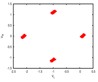
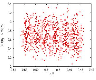
Figure 1: Allowed ranges of $V_{L}$ and $V_{R}$ NP couplings are shown in the left panel once $2\sigma$ constraint coming from the measured values of the ratio of branching ratios $R_{D}$ and $R_{D^{\ast}}$ is imposed. We show in the right panel the allowed ranges in $\mathcal{B}(B_{c}\to\tau\nu)$ and $P_{\tau}^{D^{\ast}}$ in the presence of these NP couplings.

Observables	Range	Observables	Range	Observables	Range
$\mathcal{B}(B_{c}\to\tau\nu)\times 10^{2}$	$[2.06,3.32]$	$R_{\eta_{c}}$	$[0.240,0.658]$	$P_{\tau}^{J/\Psi}$	$[-0.435,-0.491]$
$\mathcal{B}(B_{c}\to\eta_{c}\,\tau\nu)\times 10^{3}$	$[1.14,2.97]$	$R_{J/\Psi}$	$[0.300,0.413]$	$P_{\tau}^{D}$	$[0.334,0.338]$
$\mathcal{B}(B_{c}\to J/\Psi\,\tau\nu)\times 10^{3}$	$[3.12,5.09]$	$P_{\tau}^{\eta_{c}}$	$[0.141,0.530]$	$P_{\tau}^{D^{\ast}}$	$[-0.477,-0.533]$

Table 5: Allowed ranges of various observables in the presence of $V_{L}$ and $V_{R}$ NP couplings

In Fig. 2, we show the effect of $V_{L}$ and $V_{R}$ NP couplings on various observables such as ratio of branching ratio $R(q^{2})$, the forward backward asymmetry $A^{FB}(q^{2})$, and differential branching ratio ${\rm DBR}(q^{2})$ as a function of $q^{2}$ for the $B_{c}\to\eta_{c}\tau\nu$ and $B_{c}\to J/\Psi\tau\nu$ decays. We show in dark (blue) band the SM range and show in light (green) band the allowed range of each observable once the NP couplings $V_{L}$ and $V_{R}$ are switched on. We see significant deviation from the SM prediction of all the observables. The forward backward asymmetry parameter, $A^{FB}(q^{2})$, does not vary with the NP couplings $V_{L}$ and $V_{R}$ for the $B_{c}\to\eta_{c}\tau\nu$ decay mode. It is expected as the NP dependency cancels in the ratio since $B_{c}\to\eta_{c}\tau\nu$ decay mode depends on $G_{V}$ couplings only.

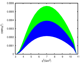
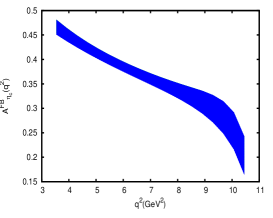
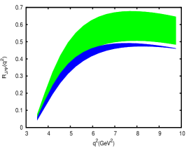
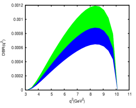
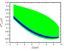
Figure 2: Range in various $q^{2}$ dependent observables such as DBR$(q^{2})$, $R(q^{2})$, and $A^{FB}(q^{2})$ for the $B_{c}\to\eta_{c}\tau\nu$  (upper panel) and $B_{c}\to J/\Psi\tau\nu$ (lower panel) decays. The allowed range is each observable is shown in light (green) band once the NP couplings $(V_{L},\,V_{R})$ are varied within the allowed ranges shown in the left panel of Fig. 1. We show in dark (blue) band the corresponding SM prediction.

III.2 Scenario II: only $S_{L}$ and $S_{R}$ type NP couplings

In this scenario, we vary only the new scalar interactions $S_{L}$ and $S_{R}$ while keeping all other NP couplings to be zero. We restrict the $S_{L}$ and $S_{R}$ parameter space using the $2\sigma$ experimental constraint coming from measured values of $R_{D}$ and $R_{D^{\ast}}$. The allowed range of $S_{L}$ and $S_{R}$ is shown in the left panel of Fig. 3. We also show in the right panel of Fig. 3 the allowed ranges of $\mathcal{B}(B_{c}\to\tau\nu)$ and $P_{\tau}^{D^{\ast}}$ in this scenario. We see significant deviation of all the observables from the SM expectation in this scenario. It is also worth mentioning that the tau polarization $P_{\tau}^{D^{\ast}}$ deviates significantly from the central value reported by BELLE. However, the uncertainty associated with the measured value of $P_{\tau}^{D^{\ast}}$ is rather large. Again, we notice that, in this scenario, the value of $\mathcal{B}(B_{c}\to\tau\nu)$ can exceed the total decay width of $B_{c}$ meson for some particular values of $S_{L}$ and $S_{R}$. We note that only $\leq 5\%$ of the total decay width of $B_{c}$ meson can be explained by semitaunic decays. However, this constraint can be relaxed upto $30\%$. If we assume that $\mathcal{B}(B_{c}\to\tau\nu)$ can not be greater than $5\%$, then although $S_{L}$ and $S_{R}$ type NP couplings can explain the anomalies in $R_{D}$ and $R_{D^{\ast}}$, it, however, can not accommodate $\mathcal{B}(B_{c}\to\tau\nu)$. Even with $30\%$ constraint, a large part of the NP parameter space prefered by $R_{D}$ and $R_{D^{\ast}}$ can be excluded. The allowed ranges of each observable obtained in the presence of $S_{L}$ and $S_{R}$ NP couplings are tabulated in Table. 6.

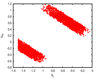
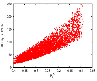
Figure 3: Allowed ranges of $S_{L}$ and $S_{R}$ NP couplings are shown in the left panel once $2\sigma$ constraint coming from the measured values of the ratio of branching ratios $R_{D}$ and $R_{D^{\ast}}$ is imposed. We show in the right panel the allowed ranges in $\mathcal{B}(B_{c}\to\tau\nu)$ and $P_{\tau}^{D^{\ast}}$ in the presence of these NP couplings.

Observables	Range	Observables	Range	Observables	Range
$\mathcal{B}(B_{c}\to\tau\nu)\times 10^{2}$	$[13.84,248.94]$	$R_{\eta_{c}}$	$[0.213,0.706]$	$P_{\tau}^{J/\Psi}$	$[-0.405,0.117]$
$\mathcal{B}(B_{c}\to\eta_{c}\,\tau\nu)\times 10^{3}$	$[1.05,3.02]$	$R_{J/\Psi}$	$[0.299,0.486]$	$P_{\tau}^{D}$	$[0.301,0.597]$
$\mathcal{B}(B_{c}\to J/\Psi\,\tau\nu)\times 10^{3}$	$[3.08,5.71]$	$P_{\tau}^{\eta_{c}}$	$[0.053,0.714]$	$P_{\tau}^{D^{\ast}}$	$[-0.090,-0.398]$

Table 6: Allowed ranges of various observables in the presence of $S_{L}$ and $S_{R}$ NP couplings

Now we wish to see the effect of $S_{L}$ and $S_{R}$ NP couplings on various $q^{2}$ dependent observables such as ratio of branching ratio $R(q^{2})$, forward backward asymmetry $A^{FB}(q^{2})$, and the differential branching ratio ${\rm DBR}(q^{2})$. The effect of NP couplings on these observables are shown in Fig. 4. Significant deviation from the SM expectation is observed for all the observables in this scenario. We see that, in this scenario, all the observables are quite sensitive to the NP couplings for $B_{c}\to\eta_{c}\tau\nu$ and $B_{c}\to J/\Psi\tau\nu$ decay modes. We also observe that, although, in the SM there is no zero crossing in the forward backward asymmetry parameter for the $B_{c}\to\eta_{c}\tau\nu$ decays; however, depending on the value of new scalar couplings $S_{L}$ and $S_{R}$, we might observe a zero crossing for this decay mode.

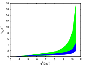
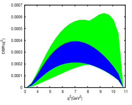
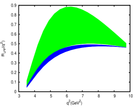
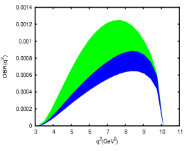
Figure 4: Range in various $q^{2}$ dependent observables such as DBR$(q^{2})$, $R(q^{2})$, and $A^{FB}(q^{2})$ for the $B_{c}\to\eta_{c}\tau\nu$  (upper panel) and $B_{c}\to J/\Psi\tau\nu$ (lower panel) decays. The allowed range is each observable is shown in light (green) band once the NP couplings $(S_{L},\,S_{R})$ are varied within the allowed ranges shown in the left panel of Fig. 3. We show in dark (blue) band the corresponding SM prediction.

III.3 Scenario III: only $\widetilde{V}_{L}$ and $\widetilde{V}_{R}$ type NP couplings

In this scenario, we wish to see the effect of right handed neutrino couplings $\widetilde{V}_{L}$ and $\widetilde{V}_{R}$ on various observables. To realize this we vary only $\widetilde{V}_{L}$ and $\widetilde{V}_{R}$ and fix all other NP couplings to zero. The allowed ranges of $\widetilde{V}_{L}$ and $\widetilde{V}_{R}$ obtained by using the $2\sigma$ constraint coming from the measured values of the ratio of branching ratios $R_{D}$ and $R_{D^{\ast}}$ are shown in the left panel of Fig. 5. The effect of $\widetilde{V}_{L}$ and $\widetilde{V}_{R}$ NP couplings on various observables are reported in Table. 7. We also show, in particular, the effect of $\widetilde{V}_{L}$ and $\widetilde{V}_{R}$ on the branching ratio of $B_{c}\to\tau\nu$ and the on tau polarization fraction $P_{\tau}^{D^{\ast}}$ in the right panel of Fig. 5. Although, very recently BELLE has reported their results on $P_{\tau}^{D^{\ast}}$, the error is quite large. More precise data on $P_{\tau}^{D^{\ast}}$ in future will help constraining the NP parameter space even more. Tau polarization fractions $P_{\tau}^{D}$ and $P_{\tau}^{\eta_{c}}$ do not vary at all with these NP couplings. It is expected since $B_{c}\to\eta_{c}\tau\nu$ and $B\to D\tau\nu$ decays depend only on $\widetilde{G}_{V}$ and hence the NP effect gets cancelled in the ratios. Deviation from the SM expectation observed in this scenario is quite similar to the deviations observed in scenario I of section. III.1.

Figure 5: Allowed ranges of $\widetilde{V}_{L}$ and $\widetilde{V}_{R}$ NP couplings are shown in the left panel once $2\sigma$ constraint coming from the measured values of the ratio of branching ratios $R_{D}$ and $R_{D^{\ast}}$ is imposed. We show in the right panel the allowed ranges in $\mathcal{B}(B_{c}\to\tau\nu)$ and $P_{\tau}^{D^{\ast}}$ in the presence of these NP couplings.

Observables	Range	Observables	Range	Observables	Range
$\mathcal{B}(B_{c}\to\tau\nu)\times 10^{2}$	$[2.11,3.39]$	$R_{\eta_{c}}$	$[0.238,0.690]$	$P_{\tau}^{J/\Psi}$	$[-0.434,-0.492]$
$\mathcal{B}(B_{c}\to\eta_{c}\,\tau\nu)\times 10^{3}$	$[1.11,3.07]$	$R_{J/\Psi}$	$[0.296,0.416]$	$P_{\tau}^{D}$	$[0.334,0.338]$
$\mathcal{B}(B_{c}\to J/\Psi\,\tau\nu)\times 10^{3}$	$[3.08,5.19]$	$P_{\tau}^{\eta_{c}}$	$[0.141,0.530]$	$P_{\tau}^{D^{\ast}}$	$[-0.474,-0.533]$

Table 7: Allowed ranges of various observables in the presence of $\tilde{V}_{L}$ and $\tilde{V}_{R}$ NP couplings

The allowed ranges of various $q^{2}$ dependent observables such as ratio of branching ratio $R(q^{2})$, the forward backward asymmetry $A^{FB}(q^{2})$, and the differential branching ratio ${\rm DBR}(q^{2})$ are shown in Fig. 6. The SM prediction is shown in dark (blue) band whereas, the effect of NP couplings is shown in light (green) band. The $q^{2}$ distribution looks quite similar to what we obtain in scenario I of section III.1. Although we see a significant deviation of all the observables in this scenario, the forward backward asymmetry parameter $A^{FB}_{\eta_{c}}(q^{2})$ for the $B_{c}\to\eta_{c}\tau\nu$ decay mode does not seem to vary with the $\tilde{V}_{L}$ and $\tilde{V}_{R}$ NP couplings. This is obvious because the $B_{c}\to\eta_{c}\tau\nu$ differential branching ratio depends only on $\widetilde{G}_{V}$ and hence the NP effect gets cancelled in the ratio. On the other hand, $B_{c}\to J/\Psi\tau\nu$ decay differntial branching ratio depends not only on $\widetilde{G}_{V}$ but also on $\widetilde{G}_{A}$ and no such cancellation of the NP effects in the forward backward asymmetry parameter occurs for this decay mode. Hence we observe a significant deviation of $A^{FB}_{J/\Psi}$ from the SM expectation.

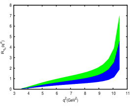
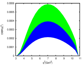
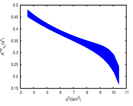
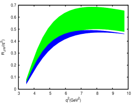
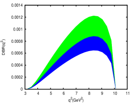
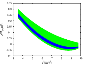
Figure 6: Range in various $q^{2}$ dependent observables such as DBR$(q^{2})$, $R(q^{2})$, and $A^{FB}(q^{2})$ for the $B_{c}\to\eta_{c}\tau\nu$  (upper panel) and $B_{c}\to J/\Psi\tau\nu$ (lower panel) decays. The allowed range is each observable is shown in light (green) band once the NP couplings $(\widetilde{V}_{L},\,\widetilde{V}_{R})$ are varied within the allowed ranges shown in the left panel of Fig. 5. We show in dark (blue) band the corresponding SM prediction.

III.4 Scenario IV: only $\widetilde{S}_{L}$ and $\widetilde{S}_{R}$ type NP couplings

To see the effect of new $\widetilde{S}_{L}$ and $\widetilde{S}_{R}$ couplings, associated with right handed neutrino, on various observables we vary $\widetilde{S}_{L}$ and $\widetilde{S}_{R}$ while keeping all other NP couplings to zero. We impose the $2\sigma$ constraint coming from the measured values of the ratio of branching ratios $R_{D}$ and $R_{D^{\ast}}$ and the resulting allowed ranges of $\widetilde{S}_{L}$ and $\widetilde{S}_{R}$ NP couplings are shown in the left panel of Fig. 7. The decay rate depends on $\widetilde{S}_{L}$ and $\widetilde{S}_{R}$ NP couplings quadratically and we obtain a less constrained NP parameter space. We also show in the right panel of Fig. 7 the allowed ranges of $\mathcal{B}(B_{c}\to\tau\nu)$ and the tau polarization fraction $P_{\tau}^{D^{\ast}}$. The branching ratio of $B_{c}\to\tau\nu$ decays obtained in this scenario is rather large; more than $45\%$. However, from the total decay width of $B_{c}$ meson one can infer that branching ratio of $B_{c}\to\tau\nu$ decays should not be more than $5\%$. Even if we relax the constraint upto $30\%$, the $\widetilde{S}_{L}$ and $\widetilde{S}_{R}$ NP couplings are ruled out although it can explain the anomalies persisted in the ratio of branching ratios $R_{D}$ and $R_{D^{\ast}}$. The allowed ranges of each observable obtained in this scenario are reported in Table. 8. All the observables are very sensitive to the new $\widetilde{S}_{L}$ and $\widetilde{S}_{R}$ NP couplings.

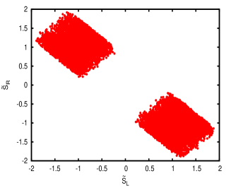
Figure 7: Allowed ranges of $\widetilde{S}_{L}$ and $\widetilde{S}_{R}$ NP couplings are shown in the left panel once $2\sigma$ constraint coming from the measured values of the ratio of branching ratios $R_{D}$ and $R_{D^{\ast}}$ is imposed. We show in the right panel the allowed ranges in $\mathcal{B}(B_{c}\to\tau\nu)$ and $P_{\tau}^{D^{\ast}}$ in the presence of these NP couplings.

Observables	Range	Observables	Range	Observables	Range
$\mathcal{B}(B_{c}\to\tau\nu)\times 10^{2}$	$[45.14,467.22]$	$R_{\eta_{c}}$	$[0.238,0.696]$	$P_{\tau}^{J/\Psi}$	$[-0.402,0.122]$
$\mathcal{B}(B_{c}\to\eta_{c}\,\tau\nu)\times 10^{3}$	$[1.10,3.15]$	$R_{J/\Psi}$	$[0.299,0.490]$	$P_{\tau}^{D}$	$[0.335,0.596]$
$\mathcal{B}(B_{c}\to J/\Psi\,\tau\nu)\times 10^{3}$	$[3.08,5.79]$	$P_{\tau}^{\eta_{c}}$	$[0.150,0.710]$	$P_{\tau}^{D^{\ast}}$	$[-0.092,-0.403]$

Table 8: Allowed ranges of various observables in the presence of $\tilde{S}_{L}$ and $\tilde{S}_{R}$ NP couplings

We wish to see the effect of these NP couplings on various $q^{2}$ dependent observables for the $B_{c}\to\eta_{c}\tau\nu$ and $B_{c}\to J/\Psi\tau\nu$ decay modes. The allowed ranges of various observables such as $R(q^{2})$, $A^{FB}(q^{2})$, and ${\rm DBR}(q^{2})$ are shown in Fig. 8. We see that all the observables deviate significantly from the SM expectation. Variation in $B_{c}\to\eta_{c}\tau\nu$ and $B_{c}\to J/\Psi\tau\nu$ decays, however, are quite different. This is what we expect because $B_{c}\to\eta_{c}\tau\nu$ decay branching ratio depends on these NP couplings through $\widetilde{G}_{S}$ term, whereas, $B_{c}\to J/\Psi\tau\nu$ decay branching ratio depend on these NP couplings through $\widetilde{G}_{P}$ term. Although the effects of $\tilde{S}_{L}$ and $\tilde{S}_{R}$ NP couplings are quite similar to $S_{L}$ and $S_{R}$ NP couplings of section. III.2, there are some differences. Unlike scenario II, we do not observe any zero crossing in the $q^{2}$ distribution of the forward backward asymmetry parameter $A^{FB}_{\eta_{c}}$ in this scenario.

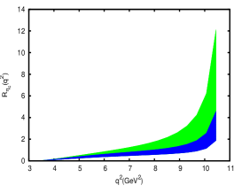
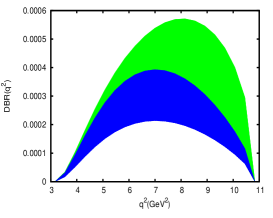
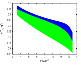
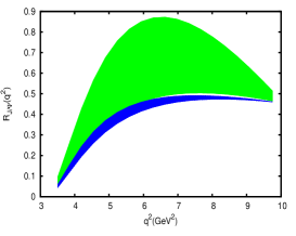
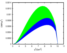
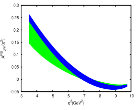
Figure 8: Range in various $q^{2}$ dependent observables such as DBR$(q^{2})$, $R(q^{2})$, and $A^{FB}(q^{2})$ for the $B_{c}\to\eta_{c}\tau\nu$  (upper panel) and $B_{c}\to J/\Psi\tau\nu$ (lower panel) decays. The allowed range is each observable is shown in light (green) band once the NP couplings $(\widetilde{S}_{L},\,\widetilde{S}_{R})$ are varied within the allowed ranges shown in the left panel of Fig. 7. We show in dark (blue) band the corresponding SM prediction.

IV Conclusion

Deviations from the SM prediction have been observed not only in decays mediated via $b\to c$ charged current process but also in decays mediated via $b\to s$ neutral current process. In particular, the deviation of the measured ratios $R_{D}$ and $R_{D^{\ast}}$ from the SM prediction is more pronounced and it currently stands at $3.9\sigma$ level. Similarly, there are significant deviations from the SM prediction in $b\to s\,l^{+}\l^{-}$ decays as well. The measured ratio $R_{K}$ deviates from the SM prediction by $2.6\sigma$. Again, various other interesting tensions between the experimental results and SM prediction have been observed in rare $B\to K^{\ast}\mu^{+}\mu^{-}$ and $B\to\phi\mu^{+}\mu^{-}$ decays. If it persists and confirmed by future experiments, these could provide the necessary information to unravel the flavor structure of beyond the SM physics. Study of $B_{c}\to\eta_{c}\tau\nu$ and $B_{c}\to J/\Psi\tau\nu$ decays is interesting because similar to $B\to(D,\,D^{\ast})\tau\nu$ decays, these decays are also mediated via $b\to c$ charged current interactions. Thus if NP is present in $B\to(D,\,D^{\ast})\tau\nu$ decays, then it would show up in these decay modes as well. A detailed study of these decay modes theoretically as well as experimentally is necessary in order to explore physics beyond the SM. Although, SM prediction of various observables related to these decay modes has been reported by various authors, NP contribution has not been studied in details. To see the effect of NP on various observables, we consider the most general effective Lagrangian in the presence of NP for the $b\to c\,l\,\nu$ process. We assume that NP is present only for the third generation leptons. We study four different NP scenarios. We summarise our results below.

We first report the central values and the $1\sigma$ ranges of all the observables within the SM. The branching ratios of $B_{c}\to\eta_{c}\tau\nu$ and $B_{c}\to J/\Psi\tau\nu$ decays are at the order of $10^{-3}$. Again, we find the branching ratio of $B_{c}\to\tau\nu$ to be of the order of $2\%$. The values of ratio of branching ratios $R_{\eta_{c}}$ and $R_{J/\Psi}$ are quite similar to the values reported in Ref. Wen-Fei:2013uea . We also give the first prediction of the tau polarization fraction $P_{\tau}^{\eta_{c}}$ and $P_{\tau}^{J/\Psi}$ for the $B_{c}\to\eta_{c}\tau\nu$ and $B_{c}\to J/\Psi\tau\nu$ decay modes.

We include vector-and scalar type NP interactions that involve both right handed as well as left handed neutrinos in our analysis and explore four different NP scenarios. In the first scenario, we consider only vector type NP interactions that involve left handed neutrinos. We vary $V_{L}$ and $V_{R}$ while keeping all other NP couplings to zero. Deviation from the SM expectation is observed for all the observables. The central value of $P_{\tau}^{D^{\ast}}$ reported by BELLE lies outside the allowed range of $P_{\tau}^{D^{\ast}}$ obtained in this scenario. However, the uncertainty associated with the measured value of $P_{\tau}^{D^{\ast}}$ is rather large. More precise data in future on $P_{\tau}^{D^{\ast}}$ will definitely help constraining the NP parameter space even more. The allowed range of $\mathcal{B}(B_{c}\to\tau\nu)$ is consistent with the total decay width of $B_{c}$ meson. We see no deviation from the SM prediction of tau polarization fraction $P_{\tau}^{D}$ and $P_{\tau}^{\eta_{c}}$ as the NP effects coming from $V_{L}$ and $V_{R}$ couplings cancel in the ratios. We also see the effect of these NP couplings on various $q^{2}$ dependent observables. Significant deviation from the SM expectation is observed once the NP couplings are included. There is, however, no deviation from the SM prediction of the forward backward asymmetry parameter $A^{FB}_{\eta_{c}}$.

In the second scenario, we consider that NP effect is due to the scalar type interactions that involves left handed neutrinos only, i.e, $S_{L,\,R}\neq 0$, whereas all other NP couplings are zero. Significant deviation from the SM expectation is observed for all the observables. It is also worth mentioning that the tau polarization $P_{\tau}^{D^{\ast}}$ deviates significantly from the central value reported by BELLE. Again, we notice that, in this scenario, for some particular values of $S_{L}$ and $S_{R}$, the value of $\mathcal{B}(B_{c}\to\tau\nu)$ exceeds the total decay width of $B_{c}$ meson. However, only less than $5\%$ of the total decay width of $B_{c}$ meson can be explained by semi(taunic) mode. Even if we relaxed the constraint upto $30\%$, a substantial part of NP parameter space can be excluded. Hence, $B_{c}$ total decay width put a severe constraint on $S_{L}$ and $S_{R}$ type NP couplings. We also see the effect of NP couplings on various $q^{2}$ dependent observables. The deviation observed in this scenario is more pronounced than the deviation observed in scenario I.

In the third scenario, we set $\widetilde{V}_{L,\,R}\neq 0$ while keeping all other NP couplings to zero. Similar to scenario I, we see significant deviation of all the observables from the SM prediction. We want to mention that, branching ratio of $B_{c}\to\tau\nu$ obtained in this scenario is consistent with the experimentally measured total decay width of $B_{c}$ meson. Again, although the central value of $P_{\tau}^{D^{\ast}}$ reported by BELLE lies outside the allowed range obtained, however, the $1\sigma$ range of the experimental value does overlap with the allowed range. More precise data on $P_{\tau}^{D^{\ast}}$ observable is needed to constrain the NP parameter even further. The deviation in various $q^{2}$ dependent observables observed in this scenario is similar to the ones that we observed in scenario I. The forward backward asymmetry parameter $A^{FB}_{\eta_{c}}$ does not vary at all as the NP dependency cancels in the ratio.

In the fourth scenario we consider only $\widetilde{S}_{L}$ and $\widetilde{S}_{R}$ type NP couplings. Again, as expected, the deviations from the SM prediction in this scenario is quite high. We notice that the branching ratio of $B_{c}\to\tau\nu$ decays obtained in this scenario is rather large; more than $45\%$. However, from the total decay width of $B_{c}$ meson one can infer that branching ratio of $B_{c}\to\tau\nu$ decays should not be more than $5\%$. Even if the constraint is relaxed upto $30\%$, the $\widetilde{S}_{L}$ and $\widetilde{S}_{R}$ NP couplings are ruled out although it can explain the anomalies persisted in the ratio of branching ratios $R_{D}$ and $R_{D^{\ast}}$. It is worth mentioning that, all the observables are very sensitive to the new $\widetilde{S}_{L}$ and $\widetilde{S}_{R}$ NP couplings, similar to scenario II. All the $q^{2}$ dependent observables are also very sensitive to the new $\widetilde{S}_{L}$ and $\widetilde{S}_{R}$ NP couplings.

In conclusion, we observe that, $B_{c}$ lifetime put a severe constraint on $S_{L,\,R}$ and $\widetilde{S}_{L,\,R}$ type NP couplings. More precise calculations of the $B_{c}$ lifetime and measurements of the branching fractions of its various decay channels in future should help constrain the NP parameter space even further. Again, the observable $P_{\tau}^{D^{\ast}}$ has the potential to distinguish between various NP scenarios once more precise data is available. At present, however, the experimental uncertainty associated with the tau polarization fraction $P_{\tau}^{D^{\ast}}$ is rather large. More precise data in future will difinitely help identifying the nature of NP. Measurement of all the observables for the $B_{c}\to\eta_{c}\tau\nu$ and $B_{c}\to J/\Psi\tau\nu$ decay modes will be crucial to explore the nature of NP patterns.

References

- (1) J. P. Lees et al. [BaBar Collaboration], Phys. Rev. Lett. 109, 101802 (2012) doi:10.1103/PhysRevLett.109.101802 [arXiv:1205.5442 [hep-ex]].
- (2) J. P. Lees et al. [BaBar Collaboration], Phys. Rev. D 88, no. 7, 072012 (2013) doi:10.1103/PhysRevD.88.072012 [arXiv:1303.0571 [hep-ex]].
- (3) M. Huschle et al. [Belle Collaboration], Phys. Rev. D 92, no. 7, 072014 (2015) doi:10.1103/PhysRevD.92.072014 [arXiv:1507.03233 [hep-ex]].
- (4) Y. Sato et al. [Belle Collaboration], Phys. Rev. D 94, no. 7, 072007 (2016) doi:10.1103/PhysRevD.94.072007 [arXiv:1607.07923 [hep-ex]].
- (5) A. Abdesselam et al., arXiv:1608.06391 [hep-ex].
- (6) R. Aaij et al. [LHCb Collaboration], Phys. Rev. Lett. 115, no. 11, 111803 (2015) Addendum: [Phys. Rev. Lett. 115, no. 15, 159901 (2015)] doi:10.1103/PhysRevLett.115.159901, 10.1103/PhysRevLett.115.111803 [arXiv:1506.08614 [hep-ex]].
- (7) Y. Amhis et al., arXiv:1612.07233 [hep-ex].
- (8) J. A. Bailey et al. [MILC Collaboration], Phys. Rev. D 92, no. 3, 034506 (2015) doi:10.1103/PhysRevD.92.034506 [arXiv:1503.07237 [hep-lat]].
- (9) H. Na et al. [HPQCD Collaboration], Phys. Rev. D 92, no. 5, 054510 (2015) Erratum: [Phys. Rev. D 93, no. 11, 119906 (2016)] doi:10.1103/PhysRevD.93.119906, 10.1103/PhysRevD.92.054510 [arXiv:1505.03925 [hep-lat]].
- (10) D. Bigi and P. Gambino, Phys. Rev. D 94, no. 9, 094008 (2016) doi:10.1103/PhysRevD.94.094008 [arXiv:1606.08030 [hep-ph]].
- (11) S. Aoki et al., arXiv:1607.00299 [hep-lat].
- (12) S. Fajfer, J. F. Kamenik and I. Nisandzic, Phys. Rev. D 85, 094025 (2012) doi:10.1103/PhysRevD.85.094025 [arXiv:1203.2654 [hep-ph]].
- (13) S. Fajfer, J. F. Kamenik, I. Nisandzic and J. Zupan, Phys. Rev. Lett. 109, 161801 (2012) [arXiv:1206.1872 [hep-ph]].;
- (14) W. S. Hou, Phys. Rev. D 48, 2342 (1993).;
- (15) A. G. Akeroyd and S. Recksiegel, J. Phys. G 29, 2311 (2003) [hep-ph/0306037].;
- (16) M. Tanaka, Z. Phys. C 67, 321 (1995) [hep-ph/9411405].;
- (17) U. Nierste, S. Trine and S. Westhoff, Phys. Rev. D 78, 015006 (2008) [arXiv:0801.4938 [hep-ph]].;
- (18) T. Miki, T. Miura and M. Tanaka, hep-ph/0210051.;
- (19) A. Wahab El Kaffas, P. Osland and O. M. Ogreid, Phys. Rev. D 76, 095001 (2007) [arXiv:0706.2997 [hep-ph]].;
- (20) O. Deschamps, S. Descotes-Genon, S. Monteil, V. Niess, S. T’Jampens and V. Tisserand, Phys. Rev. D 82, 073012 (2010) [arXiv:0907.5135 [hep-ph]].;
- (21) G. Blankenburg and G. Isidori, Eur. Phys. J. Plus 127, 85 (2012) [arXiv:1107.1216 [hep-ph]].;
- (22) G. D’Ambrosio, G. F. Giudice, G. Isidori and A. Strumia, Nucl. Phys. B 645, 155 (2002) [hep-ph/0207036].;
- (23) A. J. Buras, M. V. Carlucci, S. Gori and G. Isidori, JHEP 1010, 009 (2010) [arXiv:1005.5310 [hep-ph]].;
- (24) A. Pich and P. Tuzon, Phys. Rev. D 80, 091702 (2009) [arXiv:0908.1554 [hep-ph]].;
- (25) M. Jung, A. Pich and P. Tuzon, JHEP 1011, 003 (2010) [arXiv:1006.0470 [hep-ph]].;
- (26) A. Crivellin, C. Greub and A. Kokulu, Phys. Rev. D 86, 054014 (2012) [arXiv:1206.2634 [hep-ph]].;
- (27) A. Datta, M. Duraisamy and D. Ghosh, Phys. Rev. D 86, 034027 (2012) [arXiv:1206.3760 [hep-ph]].;
- (28) M. Duraisamy and A. Datta, JHEP 1309, 059 (2013) [arXiv:1302.7031 [hep-ph]].
- (29) M. Duraisamy, P. Sharma and A. Datta, Phys. Rev. D 90, no. 7, 074013 (2014) doi:10.1103/PhysRevD.90.074013 [arXiv:1405.3719 [hep-ph]].
- (30) B. Bhattacharya, A. Datta, D. London and S. Shivashankara, Phys. Lett. B 742, 370 (2015) doi:10.1016/j.physletb.2015.02.011 [arXiv:1412.7164 [hep-ph]].
- (31) B. Bhattacharya, A. Datta, J. P. Guvin, D. London and R. Watanabe, arXiv:1609.09078 [hep-ph].
- (32) P. Biancofiore, P. Colangelo and F. De Fazio, Phys. Rev. D 87, 074010 (2013) [arXiv:1302.1042 [hep-ph]].;
- (33) A. Crivellin, Phys. Rev. D 81, 031301 (2010) [arXiv:0907.2461 [hep-ph]].;
- (34) A. Celis, M. Jung, X. -Q. Li and A. Pich, JHEP 1301, 054 (2013) [arXiv:1210.8443 [hep-ph]].;
- (35) X. -G. He and G. Valencia, Phys. Rev. D 87, 014014 (2013) [arXiv:1211.0348 [hep-ph]].;
- (36) R. Dutta, A. Bhol and A. K. Giri, Phys. Rev. D 88, no. 11, 114023 (2013) doi:10.1103/PhysRevD.88.114023 [arXiv:1307.6653 [hep-ph]].
- (37) M. Tanaka and R. Watanabe, arXiv:1608.05207 [hep-ph].
- (38) N. G. Deshpande and X. G. He, arXiv:1608.04817 [hep-ph].
- (39) X. Q. Li, Y. D. Yang and X. Zhang, JHEP 1608, 054 (2016) doi:10.1007/JHEP08(2016)054 [arXiv:1605.09308 [hep-ph]].
- (40) D. Du, A. X. El-Khadra, S. Gottlieb, A. S. Kronfeld, J. Laiho, E. Lunghi, R. S. Van de Water and R. Zhou, Phys. Rev. D 93, no. 3, 034005 (2016) doi:10.1103/PhysRevD.93.034005 [arXiv:1510.02349 [hep-ph]].
- (41) F. U. Bernlochner, Phys. Rev. D 92, no. 11, 115019 (2015) doi:10.1103/PhysRevD.92.115019 [arXiv:1509.06938 [hep-ph]].
- (42) A. Soffer, Mod. Phys. Lett. A 29, no. 07, 1430007 (2014) doi:10.1142/S0217732314300079 [arXiv:1401.7947 [hep-ex]].
- (43) M. Bordone, G. Isidori and D. van Dyk, Eur. Phys. J. C 76, no. 7, 360 (2016) doi:10.1140/epjc/s10052-016-4202-x [arXiv:1602.06143 [hep-ph]].
- (44) D. Bardhan, P. Byakti and D. Ghosh, arXiv:1610.03038 [hep-ph].
- (45) A. K. Alok, D. Kumar, S. Kumbhakar and S. U. Sankar, arXiv:1606.03164 [hep-ph].
- (46) M. A. Ivanov, J. G. Körner and C. T. Tran, Phys. Rev. D 92, no. 11, 114022 (2015) doi:10.1103/PhysRevD.92.114022 [arXiv:1508.02678 [hep-ph]].
- (47) M. A. Ivanov, J. G. Körner and C. T. Tran, arXiv:1607.02932 [hep-ph].
- (48) S. M. Boucenna, A. Celis, J. Fuentes-Martin, A. Vicente and J. Virto, Phys. Lett. B 760, 214 (2016) doi:10.1016/j.physletb.2016.06.067 [arXiv:1604.03088 [hep-ph]].
- (49) S. M. Boucenna, A. Celis, J. Fuentes-Martin, A. Vicente and J. Virto, arXiv:1608.01349 [hep-ph].
- (50) S. Nandi, S. K. Patra and A. Soni, arXiv:1605.07191 [hep-ph].
- (51) R. Dutta and A. Bhol, arXiv:1611.00231 [hep-ph].
- (52) R. Alonso, B. Grinstein and J. Martin Camalich, arXiv:1611.06676 [hep-ph].
- (53) D. Beirevi, S. Fajfer, N. Konik and O. Sumensari, Phys. Rev. D 94, no. 11, 115021 (2016) doi:10.1103/PhysRevD.94.115021 [arXiv:1608.08501 [hep-ph]].
- (54) A. Celis, M. Jung, X. Q. Li and A. Pich, arXiv:1612.07757 [hep-ph].
- (55) F. Abe et al. [CDF Collaboration], Phys. Rev. D 58, 112004 (1998) doi:10.1103/PhysRevD.58.112004 [hep-ex/9804014].
- (56) I. P. Gouz, V. V. Kiselev, A. K. Likhoded, V. I. Romanovsky and O. P. Yushchenko, Phys. Atom. Nucl. 67, 1559 (2004) [Yad. Fiz. 67, 1581 (2004)] doi:10.1134/1.1788046 [hep-ph/0211432].
- (57) M. Pepe Altarelli and F. Teubert, Int. J. Mod. Phys. A 23, 5117 (2008) doi:10.1142/S0217751X08042791 [arXiv:0802.1901 [hep-ph]].
- (58) I. I. Y. Bigi, Phys. Lett. B 371, 105 (1996) doi:10.1016/0370-2693(95)01574-4 [hep-ph/9510325].
- (59) M. Beneke and G. Buchalla, Phys. Rev. D 53, 4991 (1996) doi:10.1103/PhysRevD.53.4991 [hep-ph/9601249].
- (60) C. H. Chang, S. L. Chen, T. F. Feng and X. Q. Li, Phys. Rev. D 64, 014003 (2001) doi:10.1103/PhysRevD.64.014003 [hep-ph/0007162].
- (61) C. Patrignani et al. [Particle Data Group], Chin. Phys. C 40, no. 10, 100001 (2016). doi:10.1088/1674-1137/40/10/100001
- (62) S. S. Gershtein, V. V. Kiselev, A. K. Likhoded and A. V. Tkabladze, Phys. Usp. 38, 1 (1995) [Usp. Fiz. Nauk 165, 3 (1995)] doi:10.1070/PU1995v038n01ABEH000063 [hep-ph/9504319].
- (63) V. V. Kiselev, A. E. Kovalsky and A. K. Likhoded, Nucl. Phys. B 585, 353 (2000) doi:10.1016/S0550-3213(00)00386-2 [hep-ph/0002127].
- (64) R. Dhir and R. C. Verma, Phys. Rev. D 79, 034004 (2009) doi:10.1103/PhysRevD.79.034004 [arXiv:0810.4284 [hep-ph]].
- (65) E. Hernandez, J. Nieves and J. M. Verde-Velasco, Phys. Rev. D 74, 074008 (2006) doi:10.1103/PhysRevD.74.074008 [hep-ph/0607150].
- (66) M. A. Ivanov, J. G. Korner and P. Santorelli, Phys. Rev. D 63, 074010 (2001) doi:10.1103/PhysRevD.63.074010 [hep-ph/0007169].
- (67) M. A. Ivanov, J. G. Korner and P. Santorelli, Phys. Rev. D 71, 094006 (2005) Erratum: [Phys. Rev. D 75, 019901 (2007)] doi:10.1103/PhysRevD.75.019901, 10.1103/PhysRevD.71.094006 [hep-ph/0501051].
- (68) M. A. Ivanov, J. G. Korner and P. Santorelli, Phys. Rev. D 73, 054024 (2006) doi:10.1103/PhysRevD.73.054024 [hep-ph/0602050].
- (69) D. Ebert, R. N. Faustov and V. O. Galkin, Phys. Rev. D 67, 014027 (2003) doi:10.1103/PhysRevD.67.014027 [hep-ph/0210381].
- (70) D. Ebert, R. N. Faustov and V. O. Galkin, Phys. Rev. D 68, 094020 (2003) doi:10.1103/PhysRevD.68.094020 [hep-ph/0306306].
- (71) D. Ebert, R. N. Faustov and V. O. Galkin, Eur. Phys. J. C 32, 29 (2003) doi:10.1140/epjc/s2003-01347-5 [hep-ph/0308149].
- (72) D. s. Du and Z. Wang, Phys. Rev. D 39, 1342 (1989). doi:10.1103/PhysRevD.39.1342
- (73) C. H. Chang and Y. Q. Chen, Phys. Rev. D 49, 3399 (1994). doi:10.1103/PhysRevD.49.3399
- (74) J. F. Liu and K. T. Chao, Phys. Rev. D 56, 4133 (1997). doi:10.1103/PhysRevD.56.4133
- (75) A. Abd El-Hady, J. H. Munoz and J. P. Vary, Phys. Rev. D 62, 014019 (2000) doi:10.1103/PhysRevD.62.014019 [hep-ph/9909406].
- (76) P. Colangelo and F. De Fazio, Phys. Rev. D 61, 034012 (2000) doi:10.1103/PhysRevD.61.034012 [hep-ph/9909423].
- (77) J. f. Sun, Y. l. Yang, W. j. Du and H. l. Ma, Phys. Rev. D 77, 114004 (2008) doi:10.1103/PhysRevD.77.114004 [arXiv:0806.1254 [hep-ph]].
- (78) W. Wang, Y. L. Shen and C. D. Lu, Phys. Rev. D 79, 054012 (2009) doi:10.1103/PhysRevD.79.054012 [arXiv:0811.3748 [hep-ph]].
- (79) C. F. Qiao and R. L. Zhu, Phys. Rev. D 87, no. 1, 014009 (2013) doi:10.1103/PhysRevD.87.014009 [arXiv:1208.5916 [hep-ph]].
- (80) Z. J. Xiao and X. Liu, Phys. Rev. D 84, 074033 (2011) doi:10.1103/PhysRevD.84.074033 [arXiv:1111.6679 [hep-ph]].
- (81) X. Liu, Z. J. Xiao and C. D. Lu, Phys. Rev. D 81, 014022 (2010) doi:10.1103/PhysRevD.81.014022 [arXiv:0912.1163 [hep-ph]].
- (82) J. F. Cheng, D. S. Du and C. D. Lu, Eur. Phys. J. C 45, 711 (2006) doi:10.1140/epjc/s2005-02453-0 [hep-ph/0501082].
- (83) J. F. Sun, D. S. Du and Y. L. Yang, Eur. Phys. J. C 60, 107 (2009) doi:10.1140/epjc/s10052-009-0872-y [arXiv:0808.3619 [hep-ph]].
- (84) W. F. Wang, Y. Y. Fan and Z. J. Xiao, Chin. Phys. C 37, 093102 (2013) doi:10.1088/1674-1137/37/9/093102 [arXiv:1212.5903 [hep-ph]].
- (85) K. K. Pathak and D. K. Choudhury, Int. J. Mod. Phys. A 28, 1350097 (2013) doi:10.1142/S0217751X13500978 [arXiv:1307.1221 [hep-ph]].
- (86) Y. K. Hsiao and C. Q. Geng, arXiv:1607.02718 [hep-ph].
- (87) T. Bhattacharya, V. Cirigliano, S. D. Cohen, A. Filipuzzi, M. Gonzalez-Alonso, M. L. Graesser, R. Gupta and H. -W. Lin, Phys. Rev. D 85, 054512 (2012) [arXiv:1110.6448 [hep-ph]].
- (88) V. Cirigliano, J. Jenkins and M. Gonzalez-Alonso, Nucl. Phys. B 830, 95 (2010) [arXiv:0908.1754 [hep-ph]].
- (89) J. G. Korner and G. A. Schuler, Z. Phys. C 46, 93 (1990).
- (90) A. Kadeer, J. G. Korner and U. Moosbrugger, Eur. Phys. J. C 59, 27 (2009) [hep-ph/0511019].