Parabolic degrees and Lyapunov exponents for hypergeometric local systems

Abstract.

Consider the flat bundle on $\mathbb{P}^{1}-\{0,1,\infty\}$ corresponding to solutions of the hypergeometric differential equation

$$\prod_{i=1}^{h}(\operatorname{D}-\alpha_{i})-z\prod_{j=1}^{h}(\operatorname{D}-\beta_{j})=0,\;\text{where}\ \operatorname{D}=z\dfrac{\operatorname{d\!}{}}{\operatorname{d\!}{z}}$$

For $\alpha_{i}$ and $\beta_{j}$ real numbers, this bundle is known to underlie a complex polarized variation of Hodge structure. Setting the complete hyperbolic metric on $\mathbb{P}^{1}-\{0,1,\infty\}$, we associate $n$ Lyapunov exponents to this bundle. We compute the parabolic degrees of the holomorphic subbundles induced by the variation of Hodge structure and study the dependence of the Lyapunov exponents in terms of these degrees by means of numerical simulations.

1. Introduction

Oseledets decomposition of flat bundles over an ergodic dynamical system is often referred to as dynamical variation of Hodge structure. In the case of Teichmüller dynamics, both Oseledets decomposition and a variation of Hodge structure (VHS) appear. Two decades ago it was observed in [Kon97] that these structures were linked, their invariants are related: the sum of the Lyapunov exponents associated to a Teichmüller curve equals the normalized degree of the Hodge bundle. This formula was studied extensively and extended to strata of abelian and quadratic differentials from then (see [FMZ14], [Kri04], [BM10], [EKZ14]). Soon this link was observed in other settings. In [KM16] it was used as a new invariant to classify hyperbolic structures and distinguish Deligne-Mostow’s non-arithmetic lattices in $\mathrm{SL}_{2}(\mathbb{C})$. In [Fil14] a similar formula was observed for higher weight variation of Hodge structures. The leitmotiv in this work is the study of the relationship between theses two structures in a broad class of examples with arbitrary weight. This family of examples will be given by hyperelliptic differential equations which yield a flat bundle endowed with a variation of Hodge structure over the sphere with three punctures. A recent article [EKMZ16] shows that the degrees of holomorphic flags of the Hodge filtration bound by below the sum of Lyapunov exponents. Our investigation will start by computing these degrees and then explore the behaviour of Lyapunov exponents through numerical simulations and their distance to the latter lower bounds. This will enable us to bring out some simple algebraic relations under which there is a conjectural equality.

Hypergeometric equations.

Let $\alpha_{1},\alpha_{2},\dots,\alpha_{n}$ and $\beta_{1},\beta_{2},\dots,\beta_{n}$ be two disjoint sequences of $n$ real numbers. We define the hypergeometric differential equation corresponding to those parameters

(1) $$\prod_{i=1}^{n}(\operatorname{D}-\alpha_{i})-z\prod_{j=1}^{n}(\operatorname{D}-\beta_{j})=0,\;\text{where}\ \operatorname{D}=z\dfrac{\operatorname{d\!}{}}{\operatorname{d\!}{z}}$$

This equation originates from a large class of special functions called generalized hypergeometric functions which satisfies it. For more details about these functions see for example [Yos97].

It is an order $n$ differential equation with three singularities at 0, 1 and $\infty$ hence the space of solutions is locally a dimension $n$ vector space away from singularities and can be seen in a geometrical way as a flat bundle over $\mathbb{P}^{1}-\{0,1,\infty\}$. This flat bundle is completely described by its monodromy matrices around singularities. We will be denoting monodromies associated to simple closed loop going counterclockwise around $0,1$ and $\infty$ by $M_{0},M_{1}$ and $M_{\infty}$. We get a first relation between these matrices observing that composing the three loops in the same order will give a trivial loop: $M_{\infty}M_{1}M_{0}=\operatorname{Id}$. The eigenvalues of $M_{0}$ and $M_{\infty}$ can be expressed with parameters of the hypergeometric equation (1) and $M_{1}$ has a very specific form as stated in the following proposition.

Proposition 1.1.

For any two sequences of real numbers $\alpha_{1},\dots,\alpha_{n}$ and $\beta_{1},\dots,\beta_{n}$,

• $M_{0}$ has eigenvalues $e^{2i\pi\alpha_{1}},\dots,e^{2i\pi\alpha_{n}}$

• $M_{\infty}$ has eigenvalues $e^{-2i\pi\beta_{1}},\dots,e^{-2i\pi\beta_{n}}$

• $M_{1}$ is the identity plus a matrix of rank one

Proof.

See Proposition 2.1 in [Fed15] or alternatively Prop. 3.2 and Theorem 3.5 in [BH89] ∎

This proposition determines the conjugacy class of the representation associated to the flat bundle $\pi_{1}\left({\mathbb{P}^{1}-\{0,1,\infty\}}\right)\rightarrow GL_{n}\left(\mathbb{R}\right)$ thanks to the rigidity of hypergeometric equations (see [BH89]). They will be computed explicitly in section 3.2.

Lyapunov exponents.

We now endow the 3 punctured sphere with its hyperbolic metric. As this metric implies an ergodic geodesic flow, for any integrable norm on the flat bundle we associate to it , using Oseledets theorem, a measurable flag decomposition of the vector bundle and $n$ Lyapunov exponents. These exponents correspond to the growth of the norm of a generic vector in each flag while transporting it along with the flat connection.

According to [EKMZ16] there is a canonical family of integrable norms on the flat bundle associated to the hypergeometric equation which will produce the same flag decomposition and Lyapunov exponents. This family contains the harmonic norm induced by the VHS structure and the norm we will use in our algorithm.

Variation of Hodge structure.

Hypergeometric equations on the sphere are well known to be physically rigid (see [BH89] or [Kat96]) and this rigidity together with irreducibility is enough to endow the flat bundle with a VHS using its associated Higgs bundle structure (see [Fed15] or directly Cor 8.2 in [Sim90]). Using techniques from [Kat96] and [DS13], Fedorov gives in [Fed15] an explicit way to compute the Hodge numbers for the underlying VHS. We extend this computation and give a combinatorial point of view that will be more convenient in the following to express parabolic degrees of the Hodge flag decomposition.

We introduce a canonical way to describe combinatorics of the intertwining of $\alpha$’s and $\beta$’s on the circle $\mathbb{R}/\mathbb{Z}$. Starting from any eigenvalue, we browse the circle counterclockwise (or in the increasing direction for $\mathbb{R}$) and denote $\alpha_{1},\dots,\alpha_{n},\beta_{1},\dots,\beta_{n}$ by order of appearance $\eta_{1},\eta_{2},\dots,\eta_{2n}$ and define $\tilde{f}\mathrel{\mathop{\mathchar 58\relax}}\mathbb{Z}\cap[0,2n]\mapsto\mathbb{Z}$ recursively by the following properties,

• $\tilde{f}(0)=0$

• $\tilde{f}(k)=\tilde{f}(k-1)+\left\{\begin{array}[]{rl}1&\text{ if }\eta_{k}\text{ is an }\alpha\\ -1&\text{ if }\eta_{k}\text{ is an }\beta\\ \end{array}\right.$

Let $f$ be defined on the eigenvalues by $f(\eta_{k})=\tilde{f}(k)$. It depends on the choice of starting point up to a shift. For a canonical definition, we shift $f$ such that its minimal value is $0$. It is equivalent to starting at the point of minimal value. This defines a unique $f$ which we intertwining diagram of the equation.

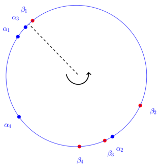
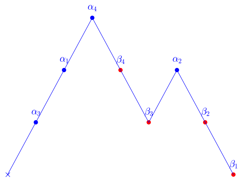
Figure 1. Example of computation of $f$

For every integer $1\leq i\leq n$ we define

$$h_{i}\mathrel{\mathop{\mathchar 58\relax}}=\#\{\alpha\ |\ f(\alpha)=i\}\ =\ \#\{\beta\ |\ f(\beta)=i-1\}$$

Then we have the following theorem,

Theorem (Fedorov).

The $h_{1},h_{2},\dots,h_{n}$ are the Hodge numbers of the VHS after an appropriate shifting.

Remark.

If the $\alpha$’s and $\beta$’s appear in an alternate order then $f(\alpha)\equiv 1$ and $f(\beta)\equiv 0$ thus their is just one element in the Hodge decomposition and the polarization form is positive definite. In other words the harmonic norm is invariant by the flat connection. This implies that Lyapunov exponents are zero.

In general, this Hodge structure endows the flat bundle with a pseudo-Hermitian form of signature $(p,q)$ where $p$ is the sum of the even Hodge numbers and $q$ the sum of the odd ones. This gives classically the fact that the Lyapunov spectrum is symmetric with respect to $0$ and that at least $|p-q|$ exponents are zero (see Appendix A in [FMZ14]).

Pushing further methods of [Fed15] and [DS13], we compute the parabolic degree of the sub Hodge bundles. This computation was done with the help of computer experiments in section 4.2 which yielded a conjectural formula for these degrees. Besides from the intertwining diagram, another quantity emerges to express them; relabel $\alpha$ and $\beta$ by order of appearance after choosing $\alpha_{1}$ such that $f(\alpha_{1})=0$, then take the representatives of $\alpha$ and $\beta$ in $\mathbb{R}$ which are included in $[\alpha_{1},\alpha_{1}+1[$ and define $\gamma\mathrel{\mathop{\mathchar 58\relax}}=\sum\beta-\sum\alpha$. The formula will depend on the floor value of $\gamma$. As $0<\gamma<n$ we have $n$ possible values $0\leq[\gamma]<n$.

Theorem 1.2.

Let $1\leq p\leq n$ and $\mathcal{E}^{p}$ the $p$-th graded piece of the Hodge filtration on $\mathbb{P}^{1}-\{0,1,\infty\}$. We denote by $\delta^{p}$ the degree of the Deligne compactification of $\mathcal{E}^{p}$ on the sphere. Then,

• if $p=[\gamma]+1$

  $$\deg_{par}(\mathcal{E}^{p})=\delta^{p}+\{\gamma\}+\sum_{f(\alpha)=p}\alpha+\sum_{f(\beta)=p-1}1-\beta$$

• otherwise

  $$\deg_{par}(\mathcal{E}^{p})=\delta^{p}+\sum_{f(\alpha)=p}\alpha+\sum_{f(\beta)=p-1}1-\beta$$

• $$-\delta^{p}(V)=\#\left\{\beta_{i}\ |\ f(\beta_{i})=p-1\text{ and }i\leq n-[\gamma]\right\}$$

Acknowledgement

I am very grateful to Maxim Kontsevich for sharing this problem and taking time to discuss it. I thank dearly Jeremy Daniel for his curiosity to the subject and his answer to my myriad of questions as well as Bertrand Deroin; Anton Zorich for his flawless support and attention, Martin Möller and Roman Fedorov for taking time to explain their understanding of the parabolic degrees and Hodge invariants at MPIM in Bonn. I am also very thankful to Carlos Simpson for his kind answers and encouragements.

2. Degree of Hodge subbundles

2.1. Variation of Hodge Structure

We start recalling the definition of complex variations of Hodge structures (VHS).

A ($\mathbb{C}$-)VHS on a curve $C$ consists of a complex local system $\mathbb{V}_{\mathbb{C}}$ with a connection $\nabla$ and a decomposition of the Deligne extension $\mathcal{V}=\bigoplus_{p\in\mathbb{Z}}\mathcal{E}^{p}$ into $C^{\infty}$-subbundles, satisfying:

• $\mathcal{F}^{p}\mathrel{\mathop{\mathchar 58\relax}}=\bigoplus_{i\geq p}\mathcal{E}^{i}$ (resp. $\overline{\mathcal{F}^{p}}\mathrel{\mathop{\mathchar 58\relax}}=\bigoplus_{i\leq p}\mathcal{E}^{i}$) are holomorphic (resp. antiholomorphic) subbundles for every $p\in\mathbb{Z}$.

• The connection shifts the grading by at most one, i.e.

  $$\nabla(\mathcal{F}^{p})\subset\mathcal{F}^{p-1}\otimes\Omega_{\mathcal{C}}^{1}\text{ and }\nabla(\overline{\mathcal{F}^{p}})\subset\overline{\mathcal{F}^{p-1}}\otimes\Omega_{\mathcal{C}}^{1}$$

Up to a shift, we can assume that there is a $n$ such that $\mathcal{E}^{i}=0$ for $i<0$ and $i>n$. We call $n$ the weight of the VHS. We can introduce for convenience the notation $\mathcal{E}^{p,n-p}\mathrel{\mathop{\mathchar 58\relax}}=\mathcal{F}^{p}/\mathcal{F}^{p-1}$. Then we have a $C^{\infty}$ isomorphism between the bundles:

$$\bigoplus_{i=0}^{n}\mathcal{E}^{i,n-i}\cong\mathbb{V}$$

2.2. Decomposition of an extended holomorphic bundle

Let $\mathcal{C}$ be a complex curve, we assume that its boundary set $\Delta\mathrel{\mathop{\mathchar 58\relax}}=\overline{\mathcal{C}}\backslash\mathcal{C}$ is an union of points. Consider $\mathcal{E}$ an holomorphic bundle on $\overline{\mathcal{C}}$. We introduce structures which will appear on such holomorphic bundle when they are obtained by canonical extension when we compactify $\mathcal{C}$. The first one will take the form of filtrations on each fibers above points of $\Delta$.

Definition 2.1 (Filtration).

A $[0,1)$-filtration on a complex vector bundle $V$ is a collection of real weights $0\leq w_{1}<w_{2}<\dots<w_{n}<w_{n+1}=1$ for some $n\geq 1$ together with a filtration of sub-vector spaces

$$G^{\bullet}\mathrel{\mathop{\mathchar 58\relax}}V=V^{\geq w_{1}}\supsetneq V^{\geq w_{2}}\supsetneq\dots\supsetneq V^{\geq w_{n+1}}=V^{\geq 1}=0$$

The filtration satisfies $V^{\geq\nu}\subset V^{\geq\omega}$ whenever $\nu\geq\omega$ and the previous weights satisfy $V^{\geq w_{i}+\epsilon}\subsetneq V^{\geq w_{i}}$ for any $\epsilon>0$.

We denote the graded vector bundles by $\operatorname{gr}_{w_{i}}\mathrel{\mathop{\mathchar 58\relax}}={\raisebox{1.99997pt}{$V^{\geq w_{i}}$}\left/\raisebox{-1.99997pt}{$V^{\geq w_{i}+\epsilon}$}\right.}$ for $\epsilon$ small. The degree of such a filtration is by definition

$$\deg(G^{\bullet})\mathrel{\mathop{\mathchar 58\relax}}=\sum_{i=1}^{n}w_{i}\dim(\operatorname{gr}_{w_{i}})$$

This leads to the next definition,

Definition 2.2 (Parabolic structure).

A parabolic structure on $\mathcal{E}$ with respect to $\Delta$ is a couple $(\mathcal{E},G^{\bullet})$ where $G^{\bullet}$ defines a $[0,1)$-filtration $G^{\bullet}\mathcal{E}_{s}$ on every fiber $\mathcal{E}_{s}$ for any $s\in\Delta$.
A parabolic bundle is a holomorphic bundle endowed with a parabolic structure.
The parabolic degree of $(\mathcal{E},G^{\bullet})$ is defined to be

$$\deg_{par}(\mathcal{E},G^{\bullet})\mathrel{\mathop{\mathchar 58\relax}}=\deg(\mathcal{E})+\sum_{s\in\Delta}\deg(G^{\bullet}\mathcal{E}_{s})$$

2.3. Deligne extension

In the following we consider $\mathbb{V}$ a flat bundle on $\mathbb{P}^{1}-\{0,1,\infty\}$ associated to a monodromy representation with norm one eigenvalues. We denote by $\mathcal{V}_{\mathcal{C}}$ the associated holomorphic vector bundle.

We recall the construction of Deligne’s extension of $\mathcal{V}_{\mathcal{C}}$ which defines a holomorphic bundle on $\overline{\mathcal{C}}$ with a logarithmic flat connection. We describe it on a small pointed disk centered at $s\in\Delta$ with coordinate $q\in D^{*}$. Let $\rho$ be a ray going outward of the singularity, then we can speak of flat sections along the ray $L(\rho)$ which has the same rank $r$ as $\mathcal{V}$. As all the $L(\rho)$ are isomorphic, we choose to denote it by $V^{0}$. There is a monodromy transformation $T\mathrel{\mathop{\mathchar 58\relax}}V^{0}\rightarrow V^{0}$ to itself obtained after continuing the solutions. This corresponds to the monodromy matrix in the given representation. For every $\alpha\in[0,1)$ we define

$$W_{\alpha}=\{v\in V^{0}\mathrel{\mathop{\mathchar 58\relax}}(T-\zeta_{\alpha})^{r}v=0\}\text{ where }\zeta_{\alpha}=e^{2i\pi\alpha}$$

These vector spaces are non trivial for finitely many $\alpha_{i}\in[0,1)$. We define

$$T_{\alpha}=\zeta_{\alpha}^{-1}T_{|W_{\alpha}}\text{ and }N_{\alpha}=\log T_{\alpha}$$

Let $q\mathrel{\mathop{\mathchar 58\relax}}\mathbb{H}\to D^{*},q(z)=e^{2i\pi z}$ be the universal cover of $D^{*}$. Choose a basis $v_{1},\dots,v_{r}$ of $V^{0}$ adapted to the generalized eigenspace decomposition $V^{0}=\bigoplus_{\alpha}W_{\alpha}$. We consider $v_{i}(z)$ as the pull back of $v_{i}$ on $\mathbb{H}$. If $v_{i}\in W_{\alpha}$, then we define

$$\widetilde{v}_{i}(z)=\exp(2i\pi\alpha z+zN_{\alpha})v_{i}$$

These sections are equivariant under $z\mapsto z+1$ hence they give global sections of $\mathcal{V}_{\mathcal{C}}(D^{*})$. The Deligne extension of $\mathcal{V}_{\mathcal{C}}$ is the vector bundle whose space of section over $D$ is the $\mathcal{O}_{\mathcal{D}}$-module spanned by $\tilde{v}_{1},\dots,\tilde{v}_{r}$. This construction naturally gives a filtration on $V^{0}$.

In general, we can define various extensions $V^{a}\subset V^{-\infty}\subset j_{*}V$ where $j$ is the inclusion $j\mathrel{\mathop{\mathchar 58\relax}}\mathcal{C}\rightarrow\overline{\mathcal{C}}$, $V^{\infty}$ is the Deligne’s meromorphic extension and $V^{a}$ (resp. $V^{>a}$) for $a\in\mathbb{R}$ is the free $\mathcal{O}_{\overline{\mathcal{C}}}$-module on which the residue of $\nabla$ has eigenvalues $\alpha$ in $[a,a+1)$ (resp. $(a,a+1]$). The bundle $V^{\bullet}$ is a filtered vector bundle in the definition of [EKMZ16].

If we have a VHS $F^{\bullet}$ on $\mathcal{E}$ over $\mathcal{C}$, it induces a filtration of every $V^{a}$ simply by taking

$$F^{p}V^{a}\mathrel{\mathop{\mathchar 58\relax}}=j_{*}F^{p}V\cap V^{a}$$

this is a well defined vector bundle thanks to Nilpotent orbit theorem (see [DS13]).

We define over some singularity $s\in\Delta$, for $a\in(-1,0]$ and $\lambda=\exp(-2i\pi a)$,

$$\psi_{\lambda}(V^{-\infty})=\operatorname{gr}_{V}^{a}={\raisebox{1.99997pt}{$V^{a}$}\left/\raisebox{-1.99997pt}{$V^{>a}$}\right.}$$

Definition 2.3 (Local Hodge data).

For $a\in[0,1)$, $\lambda=\exp(2i\pi a)$, $p\in\mathbb{Z}$ and $l\in\mathbb{N}$, we set for any $s\in\Delta$

• $\nu_{\alpha}^{p}=\dim\operatorname{gr}_{F}^{p}\psi_{\lambda}(V_{s})$ also written $h^{p}\psi_{\lambda}(V_{s})$

• $h^{p}(V)=\sum_{\alpha}\nu_{\alpha}^{p}(V_{s})$

Simpson’s theory ([Sim90]) claims that for any local system with all eigenvalues of the form $exp(-2\pi i\alpha)$ at the singularities endowed with a trivial filtration we associate a filtered $\mathcal{D}_{\overline{\mathcal{C}}}$-module with residues and jumps both equal to $\alpha$. Thus the sub $\mathcal{D}_{\overline{\mathcal{C}}}$-module corresponding to the residue $\alpha$ has only one jump of full dimension at $\alpha$, and

(2) $$\deg_{par}(\operatorname{gr}_{F}^{p}V)=\delta^{p}(V)+\sum_{s\in\Delta,\alpha}\alpha\nu_{\alpha}^{p}(V_{s})$$

where we choose $\alpha\in[0,1)$.

2.4. Acceptable metrics and metric extensions

The above Deligne extension has a geometric interpretation when we endow $\mathcal{C}$ with a acceptable metric $K$. If $V$ is a holomorphic bundle on $\mathcal{C}$, we define the sheaf $\Xi(V)_{\alpha}$ on $\mathcal{C}\cup\{s\}$ as follows. The germs of sections of $\Xi(E)_{\alpha}$ at $s$ are the sections $s(q)$ in $j_{*}V$ in the neighborhood of $s$ which satisfy a growth condition; for all $\epsilon\geq 0$ there exists $C_{\epsilon}$ such that

$$|s(q)|_{K}\leq C_{\epsilon}|q|^{\alpha-\epsilon}.$$

In general this extension is a coherent sheaf on which we do not have much information, but Simpson shows in [Sim90] that under some growth condition on the curvature of the metric, the metric induces the above Deligne extensions. When a curvature satisfies this condition it is called acceptable.

Lemma 2.4 (Lemma 2.4 [EKMZ16]).

The local system $\mathbb{V}$ with non-expanding cusp monodromies has a metric which is acceptable for its Deligne extension $\mathcal{V}$

Proof.

For completeness, we reproduce the construction of [EKMZ16]. The idea is to construct locally a nice metric and to patch the local constructions together with partition of unity. The only delicate choice is for the metric around singularities. We want the basis elements $\tilde{v}_{i}$ of the $\alpha$-eigenspace of the Deligne extension to be given the norm of order $|q|^{\alpha}$ in the local coordinate $q$ around the cusp and to be pairwise orthogonal. Let $M$ be such that $e^{2i\pi M}=T$, where $T$ is the monodromy transformation. Then the hermitian matrix $exp(log|q|\overline{M^{t}}M)$ defines a metric such that the element $\tilde{v}_{i}$ has norm $|q|^{\alpha}|\tilde{v}_{i}|$. ∎

Corollary 2.5.

When the monodromy representation goes to zero, the parabolic degree goes to zero.

Proof.

In the proof above, it is clear that when $T\to\mathrm{Id}$, $M\to 0$ and thus the metric goes to the standard hermitian metric locally. Thus its curvature goes to zero around singularities and its integral on any subbundle, which by definition is its parabolic degree, goes to zero. ∎

2.5. Local Hodge invariants

Our purpose in this subsection is to show the following relation on local Hodge invariants:

Theorem 2.6.

The local Hodge invariants for equation 1 are :

1. at $z=0$,

   $$\nu_{\alpha_{m}}^{p}=\left\{\begin{array}[]{ll}1\text{ if }p=f(\alpha_{m})\\ 0\text{ otherwise }\\ \end{array}\right.$$

2. at $z=\infty$,

   $$\nu_{-\beta_{m}}^{p}=\left\{\begin{array}[]{ll}1\text{ if }p-1=f(\beta_{m})\\ 0\text{ otherwise }\\ \end{array}\right.$$

3. at $z=1$,

   $$\nu_{\gamma}^{p}=\left\{\begin{array}[]{ll}1\text{ if }p=[\gamma]+1\\ 0\text{ otherwise }\\ \end{array}\right.$$

Remark.

Computations of (1) and (2) are done in [Fed15]. We give a similar proof with an alternative combinatoric point of view.

2.6. Computation of local Hodge invariants

In the following, we denote by $M$ the local system defined by the hypergeometric equation 1 in the introduction. The point at infinity plays a particular role in middle convolution, thus we apply a biholomorphism to the sphere which will send the three singularity points $0,1,\infty$ to $0,1,2$. Hereafter, $M$ will have singularities at $0,1,2$.

Similarly $M_{k,j}$ corresponds to the hypergeometric equation where we remove terms in $\alpha_{k}$ and $\beta_{j}$,

$$\prod_{m\neq k}(D-\alpha_{m})-z\prod_{n\neq j}(D-\beta_{n})=0$$

Let $L_{k,j}$ be a flat line bundle above $\mathbb{P}^{1}-\{0,2,\infty\}$ with monodromy $E\left(\alpha_{k}\right)$ at $0$, $E\left(-\beta_{j}\right)$ at $2$ and $E\left(\beta_{j}-\alpha_{k}\right)$ at $\infty$. Similarly $L^{\prime}_{k,j}$ is defined to have monodromy $E\left(-\beta_{j}\right)$ at $0$, $E\left(\alpha_{k}\right)$ at $2$ and $E\left(\beta_{j}-\alpha_{k}\right)$ at $\infty$.

The two key stones in the proof are Lemma $3.1$ in [Fed15] and Theorem $3.1.2$ in [DS13] :

Lemma 2.7 (Fedorov).

For any $k,j\in\{1,\dots,n\}$ we have,

$$M\simeq MC_{\beta_{j}-\alpha_{k}}\left(M_{k,j}\otimes L^{\prime}_{k,j}\right)\otimes L_{k,j}$$

We modify a little bit the formulation of [DS13], taking $\alpha=1-\alpha$. Thus the condition becomes $1-\alpha\in(0,1-\alpha_{0}]\iff\alpha\in[\alpha_{0},1)$. Which implies the following formulation.

Theorem 2.8 (Dettweiler-Sabbah).

Let $\alpha_{0}\in(0,1)$, for every singular point in $\Delta$ and any $\alpha\in[0,1)$ we have,

$$\nu^{p}_{\alpha}\left(MC_{\alpha_{0}}(M)\right)=\left\{\begin{array}[]{l l}\nu^{p-1}_{\alpha-\alpha_{0}}\left(M\right)&\text{if }\ \alpha\in\left[0,\alpha_{0}\right)\\ \nu^{p}_{\alpha-\alpha_{0}}\left(M\right)&\text{if }\ \alpha\in\left[\alpha_{0},1\right)\end{array}\right.$$

and,

$$\delta^{p}\left(MC_{\alpha_{0}}(M)\right)=\delta^{p}(M)+h^{p}(M)-\sum_{\underset{\{-\alpha\}\in[0,\alpha_{0})}{s\in\Delta}}\nu_{s,\alpha}^{p-1}(M)$$

2.6.1. Recursive argument

We apply a recursive argument on the dimension of the hypergeometric equation. Let us assume that $n\geq 3$ and that Theorem 2.6 is true for $n-1$.

For convenience in the demonstration, we change the indices of $\alpha$ and $\beta$ such that $\alpha_{i}$ (resp. $\beta_{i}$) is the $i$-th $\alpha$ (resp. $\beta$) we come upon while browsing the circle to construct the function $f$.

We apply Lemma 2.7 with $\alpha_{k}$ and $\beta_{j}$ such that $\alpha_{k}\leq\beta_{j}$. Let us describe what happens to the combinatorial function $f$ after we remove these two eigenvalues. We denote by $f^{\prime}$ the function we obtain.

Removing $\alpha_{k}$ will make the function decrease by one for the following eigenvalues until we meet $\beta_{j}$, thus for any $\tau\neq\alpha_{k},\beta_{j}$,

$$f(\tau)=\left\{\begin{array}[]{l l}f^{\prime}(\tau)&\text{if }\tau\prec\alpha_{k}\prec\beta_{j}\\ f^{\prime}(\tau)+1&\text{if }\alpha_{k}\prec\tau\prec\beta_{j}\end{array}\right.$$

(a) Graph of $f$

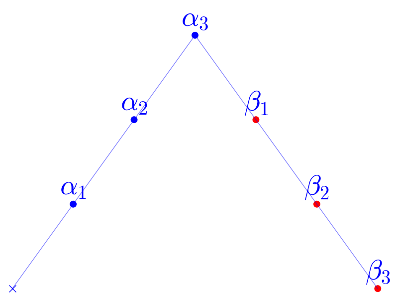
(b) Graph of $f^{\prime}$

Figure 2. Geometric representation of middle convolution action on $f$

We apply Theorem 2.8 with $\alpha_{0}=\beta_{j}-\alpha_{k}$. It yields that we have for all $m\neq k$, at singularity zero,

$$\nu^{p}_{1+\alpha_{m}-\alpha_{k}}\left(M\otimes L_{k,j}^{-1}\right)=\left\{\begin{array}[]{l l}\nu^{p-1}_{\alpha_{m}-\beta_{j}}\left(M_{k,j}\otimes L^{\prime}_{k,j}\right)&\text{if }\{\alpha_{m}-\alpha_{k}\}<\beta_{j}-\alpha_{k}\\ \nu^{p}_{\alpha_{m}-\beta_{j}}\left(M_{k,j}\otimes L^{\prime}_{k,j}\right)&\text{otherwise}\end{array}\right.$$

which can be written in a simpler form

$$\nu^{p}_{\alpha_{m}-\alpha_{k}}\left(M\otimes L_{k,j}^{-1}\right)=\left\{\begin{array}[]{l l}\nu^{p-1}_{\alpha_{m}-\beta_{j}}\left(M_{k,j}\otimes L^{\prime}_{k,j}\right)&\text{if }\alpha_{k}\prec\alpha_{m}\prec\beta_{j}\\ \nu^{p}_{\alpha_{k}-\beta_{j}}\left(M_{k,j}\otimes L^{\prime}_{k,j}\right)&\text{if }\alpha_{m}\prec\alpha_{k}\prec\beta_{j}\end{array}\right.$$

In terms of $M$ and $M_{k,j}$,

$$\nu^{p}_{\alpha_{m}}\left(M\right)=\left\{\begin{array}[]{l l}\nu^{p-1}_{\alpha_{m}}\left(M_{k,j}\right)&\text{if }\alpha_{k}\prec\alpha_{m}\prec\beta_{j}\\ \nu^{p}_{\alpha_{m}}\left(M_{k,j}\right)&\text{if }\alpha_{m}\prec\alpha_{k}\prec\beta_{j}\end{array}\right.$$

For any integer $i,j$ we denote by $\delta(i,j)$ the function which is $1$ when $i=j$ and is zero otherwise.

$$\nu^{p}_{\alpha_{m}}\left(M\right)=\left\{\begin{array}[]{l l}\delta\left(p-1,f^{\prime}(\alpha_{m})\right)&\text{if }\alpha_{k}\prec\alpha_{m}\prec\beta_{j}\\ \delta\left(p,f^{\prime}(\alpha_{m})\right)&\text{if }\alpha_{m}\prec\alpha_{k}\prec\beta_{j}\end{array}\right.\ =\delta\left(p,f(\alpha_{m})\right)$$

Similarly for all $m\neq j$, at singularity 2,

$$\nu^{p}_{-\beta_{m}}\left(M\right)=\left\{\begin{array}[]{l l}\nu^{p-1}_{-\beta_{m}}\left(M_{k,j}\right)&\text{if }\alpha_{k}\prec\beta_{j}\prec\beta_{m}\\ \nu^{p}_{-\beta_{m}}\left(M_{k,j}\right)&\text{if }\alpha_{k}\prec\beta_{m}\prec\beta_{j}\end{array}\right.$$

$$\nu^{p}_{\beta_{m}}\left(M\right)=\left\{\begin{array}[]{l l}\delta\left(p-1,f^{\prime}\left(\beta_{m}\right)\right)&\text{if }\alpha_{k}\prec\beta_{j}\prec\beta_{m}\\ \delta\left(p,f^{\prime}\left(\beta_{m}\right)\right)&\text{if }\alpha_{k}\prec\beta_{m}\prec\beta_{j}\end{array}\right.=\delta\left(p,f\left(\beta_{k}\right)\right)$$

And at 1, we set $\tilde{\gamma}\mathrel{\mathop{\mathchar 58\relax}}=\gamma-\beta_{j}+\alpha_{k}=\sum_{m\neq j}\beta_{m}-\sum_{m\neq k}\alpha_{m}$,

$$\nu^{p}_{\gamma}\left(M\right)=\left\{\begin{array}[]{l l}\nu^{p-1}_{\tilde{\gamma}}\left(M_{k,j}\right)&\text{if }\{\gamma\}<\beta_{j}-\alpha_{k}\\ \nu^{p}_{\tilde{\gamma}}\left(M_{k,j}\right)&\text{otherwise}\end{array}\right.$$

$$\nu^{p}_{\gamma}\left(M\right)=\left\{\begin{array}[]{l l}\delta\left(p-1,[\tilde{\gamma}]+1\right)&\text{if }\{\gamma\}=\{\tilde{\gamma}\}+\beta_{j}-\alpha_{k}-1\\ \delta\left(p,[\tilde{\gamma}]+1\right)&\text{if }\{\gamma\}=\{\tilde{\gamma}\}+\beta_{j}-\alpha_{k}\end{array}\right.\ =\delta\left(p,[\gamma]+1\right)$$

Now if we choose to pick $\beta_{n}>\alpha_{n}$ for the computation, we now hodge invariants for all values excepts for $\alpha_{n}$ and $\beta_{n}$. We will use the computation with for example $\alpha_{1}<\beta_{1}$. From this one we can deduce the invariants at $\beta_{n}$ and $\alpha_{n}$. Yet, we should keep in mind that the previous computations are always modulo shifting of the VHS. That is why we need to have dimension at least $3$, since in this case $\alpha_{2}$ will appear in both computations and will show there is no shift in our formulas.

2.6.2. Initialization for n = 2

We use the computations performed in the previous part for $\alpha_{2}$ and $\beta_{2}$. To do so, first remark that the unique (complex polarized) VHS on $M_{2,2}$ is defined by $h^{p}\left(M\right)=\delta(p,1)$ and the only non-zero local Hodge invariants are

$$\begin{array}[]{l l l}\nu_{\alpha_{1}}^{1}\left(M_{2,2}\right)&=1&\text{at singularity }0\\ \nu_{-\beta_{1}}^{1}\left(M_{2,2}\right)&=1&\text{at singularity }\infty\\ \nu_{\beta_{1}-\alpha_{1}}^{1}\left(M_{2,2}\right)&=1&\text{at singularity }1\\ \end{array}$$

Which corresponds to the definition of $\delta(p,f^{\prime}(\alpha_{1}))$ for the first two, and to $\delta(p,[\gamma]+1)$ for the last one.

Using the previous subsection, we deduce

$$\begin{array}[]{l l l}\nu_{\alpha_{1}}^{p}\left(M\right)&=\delta(p,f(\alpha_{1}))&\text{at singularity }0\\ \nu_{-\beta_{1}}^{p}\left(M\right)&=\delta(p,f(\alpha_{1}))&\text{at singularity }\infty\\ \nu_{\gamma}^{p}\left(M\right)&=\delta(p,[\gamma]+1)&\text{at singularity }1\\ \end{array}$$

According to [Fed15], the Hodge numbers on $M$ are

$$h^{1}=\left\{\begin{array}[]{l l}1&\text{if }\alpha_{1}\prec\alpha_{2}\prec\beta_{1}\prec\beta_{2}\\ 2&\text{if }\alpha_{1}\prec\beta_{1}\prec\alpha_{2}\prec\beta_{2}\end{array}\right.,\hskip 28.45274pth^{2}=\left\{\begin{array}[]{l l}1&\text{if }\alpha_{1}\prec\alpha_{2}\prec\beta_{1}\prec\beta_{2}\\ 0&\text{if }\alpha_{1}\prec\beta_{1}\prec\alpha_{2}\prec\beta_{2}\end{array}\right.$$

Using the fact that $\sum_{\alpha}\nu^{p}_{\alpha}=h^{p}$, we can deduce the other Hodge invariants.

$$\begin{array}[]{l l}\nu_{\alpha_{2}}^{2}=1&\text{if }\alpha_{1}\prec\alpha_{2}\prec\beta_{1}\prec\beta_{2}\\ \nu_{\alpha_{2}}^{1}=1&\text{if }\alpha_{1}\prec\beta_{1}\prec\alpha_{2}\prec\beta_{2}\end{array}$$

We conclude that $\nu_{\alpha_{2}}^{p}\left(M\right)=\delta(p,f(\alpha_{2}))$ and similarly $\nu_{-\beta_{2}}^{p}\left(M\right)=\delta(p,f(\alpha_{2}))$.

2.7. Continuity of the parabolic degree

To compute $\delta^{p}(V)$ in equation 2, we show in the following Lemma a continuity property which implies that it is constant on a given domain.

Lemma 2.9.

Let $\alpha_{1},\dots,\alpha_{n},\beta_{1},\dots,\beta_{n}$ be all disjoint, not integers and such that $\gamma$ also is not an integer. Fix the intertwining diagram of $\alpha$ and $\beta$ and the value of $[\gamma]$, then for any integer $p$, $\delta^{p}(V)$ is constant.

Proof.

Let $L$ and $L^{\prime}$ be the local system corresponding to equation 1 for eigenvalues $\alpha,\beta$ (resp. $\alpha^{\prime},\beta^{\prime}$) satisfying the above hypothesis. We endow them with a trivial filtration. According to Simpson’s theory, $L$ corresponds to some Higgs bundle $(E,\theta)$ together with a parabolic structure at singularities. As $L$ has eigenvalues of norm one, $\theta$ has no residue, moreover its weight filtration is locally the same as the one for the unipotent part of monodromy matrices of $L$.

Consider now $(E^{\prime},\theta^{\prime})$ a Higgs bundle with the same holomorphic structure and Higgs form as $(E,\theta)$ but a slightly changed parabolic structure for which we keep the initial filtration but modify the parabolic weights $\alpha,\beta$ to $\alpha^{\prime},\beta^{\prime}$. It is clear that we keep the same residues $\mathrm{res}_{s}(\theta)=\mathrm{res}_{s}(\theta^{\prime})$ at every singularity $s$. We also keep locally the same weight filtration for the unipotent part of the monodromy on any eigenspace. This implies that monodromy matrices of the local system associated to $(E^{\prime},\theta^{\prime})$ and those of $L^{\prime}$ are locally isomorphic, and by rigidity of the hypergeometric local systems they are globally isomorphic. The same argument applies for Hodge subbundles. As the considered domain is connected this shows that the parabolic degree of the Hodge subbundles is constant. ∎

Together with Corollary 2.5 this is enough to compute $\delta^{p}(V)$. We fix an intertwining diagram and a floor value for $\gamma$ and make the first $[\gamma]$ $\beta$ go to $1$ and the rest of eigenvalues to $0$ while staying in the given domain. At the limit, the parabolic degree is zero and we can deduce $\delta^{p}(V)$.

3. Algorithm

In this section, we describe the algorithm used to compute the Lyapunov exponents. We start simulating a generic hyperbolic geodesic and following how it winds around the surface, namely the evolution of the homology class of the closed path. Finally we compute the corresponding monodromy matrix after each turn around a cusp.

3.1. Hyperbolic geodesics

This first question arising to unravel this computation of Lyapunov exponents is how to simulate a generic hyperbolic geodesic. The answer comes from a beautiful theorem proved by Caroline Series in [Ser85] which relates hyperbolic geodesics on the Poincaré half-plane and continued fraction development of real numbers. We follow here the notations of [Dal07] (see part II.4.1).

Let us consider the Farey tessellation of $\mathbb{H}$ (see Figure 3).

Figure 3. The Farey’s tessellation

It is the fundamental domain for the discrete subgroup of index $3$ in $\operatorname{PSL}\left(\mathbb{Z}\right)$ generated by

$$\left<\left(\begin{array}[]{cc}1&1\\ 0&1\end{array}\right),\left(\begin{array}[]{cc}1&0\\ 1&1\end{array}\right)\right>$$

The sphere minus three points endowed with its complete hyperbolic metric is a degree two cover of the surface associated to Farey’s tessellation. This is why we represent the tessellation with two colors : the fundamental domain for the sphere corresponds to two adjacent triangles of different colors. That is why it will be easy once we understand the geodesics with respect to this tessellation to see them on the sphere.

Let us consider a geodesic going through $i$. It lands to the real axis at a positive and a negative real number. The positive real number will be called $x$, this number determines completely the geodesic since we know two distinct points on it.

We associate to this geodesic a sequence of positive integers. Look at the sequence of hyperbolic triangles the geodesic will cross. For each one of those triangles, the geodesic has two ways to cross them (see Figure 3). Once it enters it, it can leave it crossing either the side of the triangle to its left (a) or to its right (b).

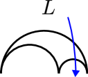
(a) to the left

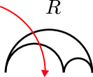
(b) to the right

Figure 4. Two ways to cross an hyperbolic triangle

Remark.

The vertices of hyperbolic triangles are located at rational numbers, so this sequence will be infinite if and only if $x$ is irrational (see [Dal07] Lemme 4.2).

We have now for a generic geodesic an infinite word in two letters $L$ and $R$ associated to a geodesic. For example the word associated to the geodesic in Figure 5, is of the form $LLRRLR\dots=L^{2}R^{2}L^{1}R\dots$. We can factorize each of those words and get

$$R^{n_{0}}L^{n_{1}}R^{n_{2}}L^{n_{3}}\dots$$

Except for $n_{0}$ which can be zero the $n_{i}$ are positive integers.

Theorem 3.1.

The sequence $(n_{k})$ is the continued fraction development of $x$. In other words,

$$x=n_{0}+\cfrac{1}{n_{1}+\cfrac{1}{n_{2}+\cfrac{1}{n_{3}+\dots}}}$$

The measure induced on the real axis by the measure on $T^{1}\mathbb{H}$ dominates Lebesgue measure.

See [Dal07] II.4 or [Ser85] for a proof.

Remark.

This theorem states exactly that to study a generic geodesic on the hyperbolic plane, we can consider a Lebesgue generic number in $(0,\infty)$ and compute its continued fraction development.

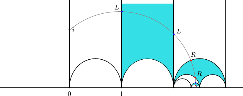
Figure 5. Crossings of a given geodesic

To compute Lyapunov exponents of the flat bundle, we need to follow how a generic geodesic winds around the cusps. By the previous theorem we can simulate a generic cutting sequence of an hyperbolic geodesic in $\mathbb{H}$. Our goal now will be to associate to such a sequence a product of monodromy matrices following its homotopy class.

Since we will consider universal cover of the sphere minus three points, for convenience we will denote by $A$, $B$, $C$ the cusps corresponding in the surface to $\infty$, $0$, $1$ respectively and use this latter notation for points in $\mathbb{H}$. Two adjacent hyperbolic triangles of Farey’s tessellation, e.g. $0,1,\infty$ and $1,2,\infty$ will form a fundamental domain for this surface. All the vertices of the hyperbolic triangles for this tessellation are associated to either $A,B$ or $C$. To follow how the flow turns around these vertices in the surface, we will need to keep track of orientation. To do so, we color the triangles according to the order of its vertices, when we browse the three vertices counterclockwise if we have $A\rightarrow B\rightarrow C\rightarrow A$ we color the triangle in white (this is the case for $0,1,\infty$) otherwise we color it in blue (case of $\infty,2,1$).

Let us now consider a point $P$ inside the blue triangle, which will be used as a base point for an expression of the cycles around cusps. We choose a homology marking of the surface by denoting the paths going around $A$, $B$, $C$ counterclockwise starting and ending at $P$,   $a$, $b$, $c$ (see Figure 6). When we concatenate these paths we get $c\cdot b\cdot a=\operatorname{Id}$ and $a^{-1}=c\cdot b$. For monodromy matrices we will have the relation

(3) $$M_{\infty}M_{0}M_{1}=\operatorname{Id}$$

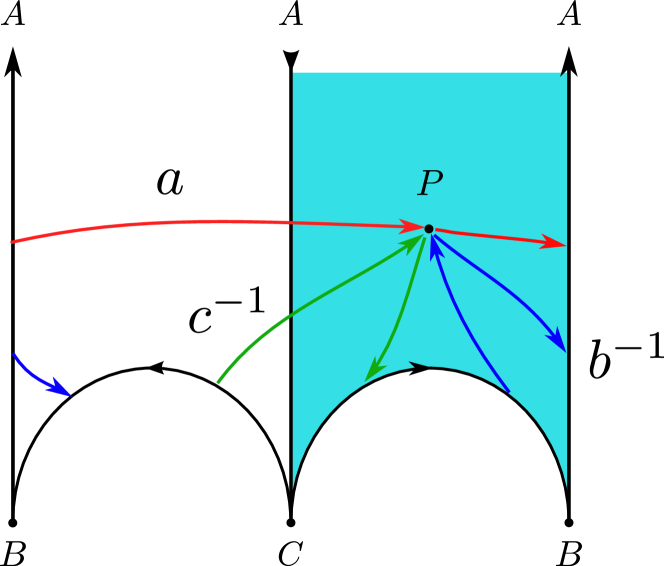
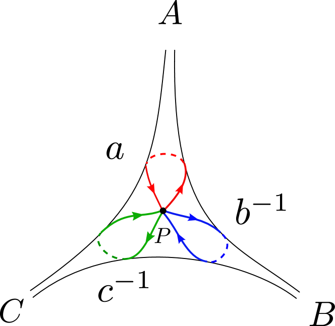
Figure 6. Homology marking

In our algorithm we will always follow the cutting sequence until we end up to a blue triangle. Then we will apply an isometry that take the fundamental domain we are in to the $(-1,0,\infty)$ triangle and the edge the flow will cut when going out of the triangle to be the $(0\infty)$ or $(-1,\infty)$ edge in order to place the cusp we are turning around at $\infty$. We shall warn the reader here that the corresponding cusp on the surface here at points $-1,0$ and $\infty$ may be any of the points $A,B,C$ but their cyclic order will stay unchanged thanks to the orientation. Thus we just need to keep track of the cusp placed at $\infty$.

When we start with a cutting sequence extracted from the previous theorem we see that the geodesic start by cutting $(0,\infty)$ at $i$ without being counted in the cutting sequence. The first cutting will always be forgotten in the sequence when applying the isometry.

Now remark that when the crossing is a sequence of $2n$ left, we make $n$ turns counterclockwise around the cusp placed at $\infty$. When it $2n$ right, we make $n$ turn clockwise. It is a little trickier if the geodesic makes an odd number of the same crossing; we need to take one step further from the next term in the sequence of crossings to end up at $P$ (see Figure 7).

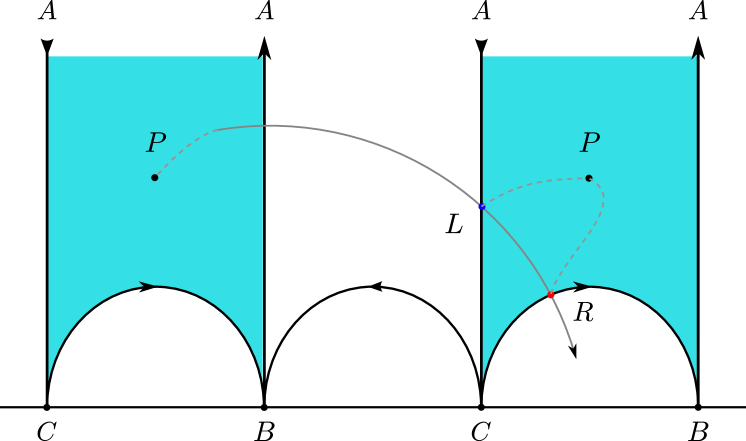
(a) Odd number of sections

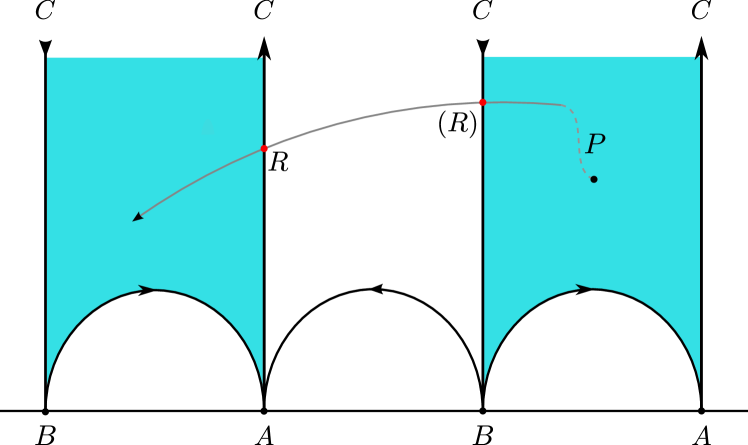
(b) Changing the setting

Figure 7. Applying the good orientation preserving isometry

There is a last point to consider, since we want to compare the growth of the harmonic norm with regards to the geodesic flow, need to follow its length. Here the discretized algorithm enables us to follow the type of homotopy it will have, but the length will not correspond a priori to the number of iterations of our algorithm. It is proportional to it by the constant.

3.2. Monodromy matrices

In the introduction Proposition 1.1 gave a set of three properties on the monodromy matrices for the hypergeometric differential equation associated to two distinct sequences of real numbers $\alpha_{1},\dots,\alpha_{n}$ and $\beta_{1},\dots,\beta_{n}$. We claim that those properties are sufficient to recover the monodromy matrices up to conjugacy.

For convenience we always assume that the $\alpha_{1},\dots,\alpha_{n}$ are disjoint, otherwise the computation becomes way more tedious, and in our computations we will explore generic domains. We choose a basis in which $M_{0}$ is diagonal. Property (3) tells us that $M_{1}-\operatorname{Id}$ is of rank $1$. We can then find two vectors $v$ and $w$ such that $M_{1}=\operatorname{Id}+vw^{t}$.

Since $M_{\infty}^{-1}=M_{0}M_{1}$ knowing the eigenvalues of $M_{\infty}$ we can derive the following $n$ equations, for all $j$,

$$\det\left(M_{\infty}^{-1}-e^{2i\pi\beta_{j}}\operatorname{Id}\right)=0\\$$

We can compute this determinant using the particular form of the matrix and the following lemma.

$$M_{0}M_{1}-e^{2i\pi\beta_{j}}\operatorname{Id}=(M_{0}-e^{2i\pi\beta_{j}}\operatorname{Id})+(M_{0}v)w^{t}$$

We can conjugate by diagonal matrices so that $M_{0}v$ becomes the vector $\mathbb{1}$ which is one on every coordinates. And obtain the equations

$$\det((M_{0}-e^{2i\pi\beta_{j}}\operatorname{Id})+\mathbb{1}w^{t})=0,\;\forall j$$

Lemma.

Let $D$ a diagonal matrix with $d_{1},\dots,d_{n}$ on its diagonal, and $x$ a vector.

$$\det\left(D+\mathbb{1}x^{t}\right)=\left(\prod_{i=1}^{n}d_{i}\right)\cdot\left(1+\sum_{i=1}^{n}x_{i}/d_{i}\right)$$

Proof.

First consider the case where $D$ is the identity matrix. We know that all the eigenvalues except for one are 1. The determinant will then be the eigenvalue of an eigenvector which image through $x^{t}$ is not zero. This vector will be $\mathbb{1}$ and its eigenvalue $(1+\sum_{i=1}^{n}x_{i})$. To finish the proof, just factor each column by $d_{i}$ in the determinant. ∎

We obtain

$$\left(\prod_{i=1}^{n}e^{2i\pi\alpha_{i}}-e^{2i\pi\beta_{j}}\right)\left(1+\sum_{i=1}^{n}\frac{w_{i}}{e^{2i\pi\alpha_{i}}-e^{2i\pi\beta_{j}}}\right)=0$$

Corollary.

The vector $w$ satisfies for all $j$,

$$\sum_{i=1}^{n}\frac{w_{i}}{e^{2i\pi\beta_{j}}-e^{2i\pi\alpha_{i}}}=1$$

We define a matrix $N=\left(\frac{1}{e^{2i\pi\beta_{j}}-e^{2i\pi\alpha_{i}}}\right)_{i,j}$ and observe that $w^{t}N=\mathbb{1}^{t}$ so $w^{t}=\mathbb{1}^{t}N^{-1}$. Hence for a generic setting, we just have to invert $N$ to find the explicit monodromies. And finally we have the expression $M_{1}=\operatorname{Id}+M_{0}^{-1}\mathbb{1}\cdot\mathbb{1}^{t}N^{-1}$

4. Observations

4.1. Calabi-Yau families example

A first family of examples is coming from 14 1-dimensional families of Calabi-Yau varieties of dimension $3$. The Gauss-Manin connection for this family on its Hodge bundle gives an example of the hypergeometric family we are considering. The monodromy matrices were computed explicitly in [ES08] and have a specific form parametrized by two integers $C$ and $d$. We introduce the following monodromy matrices,

$$T=\left(\begin{array}[]{cccc}1&0&0&0\\ 1&1&0&0\\ 1/2&1&1&0\\ 1/6&1/2&1&1\\ \end{array}\right)\hskip 28.45274ptS=\left(\begin{array}[]{cccc}1&-C/12&0&-d\\ 0&1&0&0\\ 0&0&1&0\\ 0&0&0&1\\ \end{array}\right)$$

In the previous notations, $M_{0}=T,M_{1}=S,M_{\infty}=(TS)^{-1}$. These matrices satisfy relation 3, $M_{\infty}M_{0}M_{1}=\operatorname{Id}$. We see that $M_{1}-\operatorname{Id}$ has rank one and eigenvalues of $M_{0}$ and $M_{\infty}$ have module one thus correspond to hypergeometric equations. In this setting, $T$ has eigenvalues all equal to one and eigenvalues of $(TS)^{-1}$ are symmetric with respect to zero, we denote them by $\mu_{1},\mu_{2},-\mu_{2},-\mu_{1}$ where $\mu_{1},\mu_{2}\geq 0$.

The parabolic degree of the holomorphic Hodge subbundles are given by,

Theorem.

[EKMZ16] Suppose $0<\mu_{1}\leq\mu_{2}\leq 1/2$ then the degree of the Hodge bundles are

$$\deg_{par}\mathcal{E}^{3,0}=\mu_{1}\ \text{ and }\ \deg_{par}\mathcal{E}^{2,1}=\mu_{2}$$

Thus according to the same article, we know that $2(\mu_{1}+\mu_{2})$ is a lower bound for the sum of Lyapunov exponents. We call good cases the equality cases and bad cases the cases where there is strict inequality.

There are 14 different couples of values for $C$ and $d$ where the corresponding flat bundle is an actual Hodge bundle over a family of Calabi-Yau varieties. These examples where computed few year ago by M. Kontsevich and were a motivation for this article. We list them in the table below.

C	d	$\lambda_{1}+\lambda_{2}$	$\lambda_{1}$	$\mu_{1},\mu_{2}$
46	1	1	0.97	1/12, 5/12
44	2	1	0.95	1/8, 3/8
52	4	4/3	1.27	1/6, 1/2
50	5	6/5	1.12	1/5, 2/5
56	8	3/2	1.40	1/4, 1/2
60	12	5/3	1.53	1/3, 1/2
64	16	2	1.75	1/2, 1/2

(a) The 7 good cases

C	d	$\lambda_{1}+\lambda_{2}$	$\lambda_{1}$	$\mu_{1},\mu_{2}$
22	1	0.92	0.75	1/6, 1/6
34	1	0.83	0.77	1/10, 3/10
32	2	0.97	0.84	1/6, 1/4
42	3	1.06	0.96	1/6, 1/3
40	4	1.30	1.07	1/4, 1/4
48	6	1.31	1.15	1/4, 1/3
54	9	1.60	1.34	1/3, 1/3

(b) The 7 bad cases

Figure 8. Experiments

To see what happens in a similar setting for more general hypergeometric equations, we vary $C,d$ and compute the corresponding eigenvalues $\mu_{1}$ and $\mu_{2}$ as well as the Lyapunov exponents. On Figure 9(a) we drew a blue point at coordinate $(\mu_{1},\mu_{2})$ if the sum of positive Lyapunov exponents are as close to the parabolic degree $2(\mu_{1}+\mu_{2})$ as the precision we have numerically and we put a red point when this value is outside of the confidence interval.

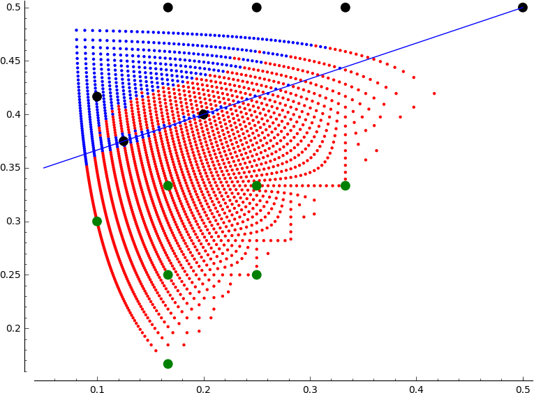
(a) The good and bad cases

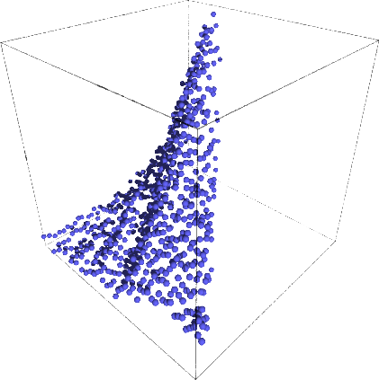
(b) Zoom on the part above the line

Figure 9. Experiments

Note that according to Figure 9(a) it seems that all points below the line of equation $3\mu_{2}=\mu_{1}+1$ are bad cases. In Figure 9(b), we represent the distance of the sum of the Lyapunov exponents to the expected formula. We see that this gives a function that oscillates above zero. More precisely, it seems that good cases are outside of some lines passing through $(1/2,1/2)$.

To push the numerical simulations further, we consider what happens on lines of equation $3\mu_{2}=\mu_{1}+1$ 10(a) and $48\mu_{2}=10\mu_{1}+19$ 10(b) both passing through $(1/2,1/2)$ and a point corresponding to one of the previous good cases.

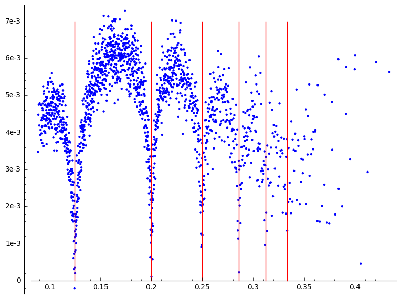
(a) $3\mu_{2}=\mu_{1}+1$

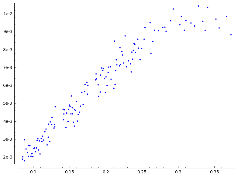
(b) $48\mu_{2}=10\mu_{1}+19$

Figure 10. Lyapunov exponents in function of $\mu_{1}$

We observe that on the graph 10(b) there is only one good case which corresponds to $(\mu_{1},\mu_{2})=(1/10,3/10)$ in the previous list of good cases. In the graph 10(a), there are good cases at points $(\mu_{1},\mu_{2})=(1/8,3/8),(1/5,2/5)$ which were also on the previous list but other points appear such as $(3/12,5/12),(5/16,7/16),(3/9,4/9)$.

According to [BT14] and [SV14], the 7 good cases correspond to cases where the monodromy group of the hypergeometric local system is of infinite index in $Sp(4,\mathbb{Z})$, which is commonly called thin. In the other cases the group is of finite index and is called thick. The three good cases we found by ways of Lyapunov exponents do not seem to have a representation with integers $C$ and $d$. A lot of questions arise about these points, for example can we find a number-theoretic interpretation of their equality as in Conjecture 6.5 in [EKMZ16].

4.2. Examples for $n=2$

Has we have seen in the introduction the two Lyapunov exponents are symmetric $\lambda_{1}$ and $-\lambda_{1}$. The sum of the positive Lyapunov exponents is just $\lambda_{1}$. The parameter space we have for these $2$-dimensional flat bundles are $\alpha_{1},\alpha_{2},\beta_{1},\beta_{2}$.

The Lyapunov exponents are invariant through translation of the set of parameters. Indeed, we can consider the bundle with $e^{\delta}M_{0}$ and $e^{-\delta}M_{\infty}$ monodromies, it will have the same set of Lyapunov exponents since both scalar will appear with the same frequency and its parameters will be $\alpha_{1}+\delta,\dots,\alpha_{h}+\delta,\beta_{1}+\delta,\dots,\beta_{h}+\delta$ hence without loss of generality we can assume $\beta_{1}=0$. Moreover the parameters are given as a set, the order does not matter.

In the following experiments we will consider a set of parameters where the $\beta$’s will be equidistributed and the $\alpha$’s will be shifted with respect to them. Here we represent the value of the Lyapunov exponent for $\alpha_{1}=r,\alpha_{2}=2r,\beta_{1}=0,\beta_{2}=x$ and we have by definition $\gamma=x-3r$.

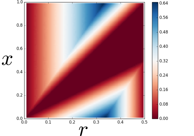
(a) Plotting $\lambda_{1}$

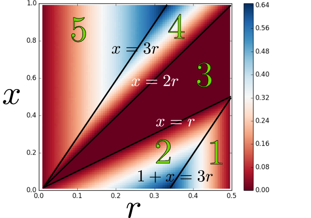
(b) Zones on the graph

Figure 11. Experiments

Remark.

We first notice that the zone where the Lyapunov exponent is zero corresponds to the setting where the parameters are alternate and where there is a positive definite bilinear form invariant by the flat connection (see introduction). This will be true whenever the VHS has weight $0$.

Another noticeable fact is that zones correspond exactly to different combinatorics for the order of the $\alpha$ and $\beta$, and on $[\gamma]$ introduced in the introduction.

(a) Diagram for zones 1 and 2

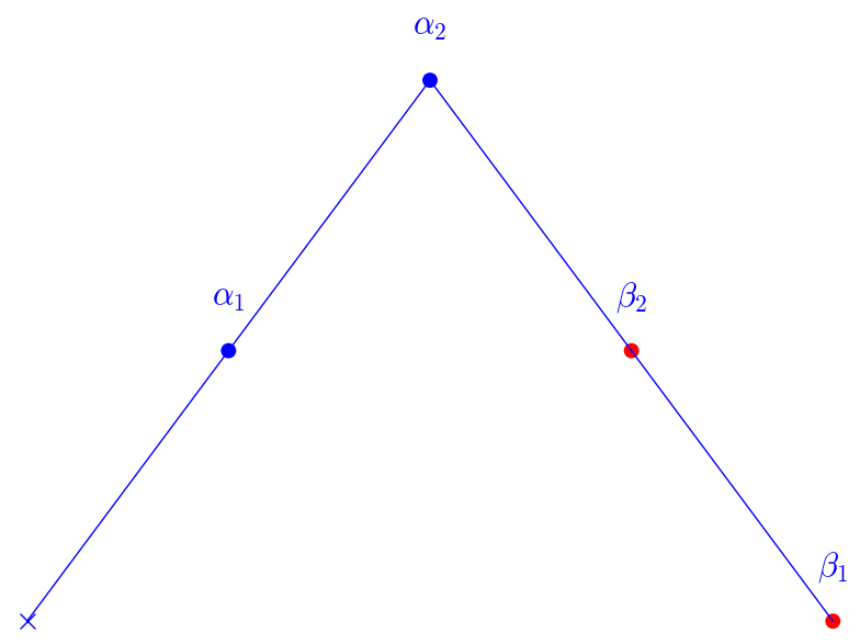
(b) Diagram for zones 4 and 5

Remark that $[\gamma]$ is $0$ in zones $1,4$, and $1$ in zones $2,5$. In the following table, we give a relation binding $\lambda_{1},r,x$ obtained by linear regression. The other column is the formula for the parabolic degree in the given zone.

Zone	$\lambda_{1}$	$\deg_{par}H^{1,0}$
1	$2(1-2r)$	$-1+\{\gamma\}+\alpha_{1}+1-\beta_{2}$
2	$2(r-x)$	$\alpha_{1}+1-\beta_{2}$
3	$0$	$0$
4	$2(x-2r)$	$-1+\{\gamma\}+\alpha_{1}+1-\beta_{1}$
5	$2r$	$\alpha_{1}+1-\beta_{1}$

In this case, the VHS is of weight $\leq 1$ and thus is in the setting of [Kon97]. In consequence, we have the equality

$$\lambda_{1}=2\frac{\deg_{par}{\mathcal{E}^{1}}}{\chi(S)}$$

Where $\deg_{par}$ is the parabolic degree of the holomorphic bundle and $\chi(S)=1$ the Euler characteristic of $S$.

This is a good test for our algorithm and formula on degree. More generally, for any dimension $n$, this formula will hold as long as the weight is equal to $1$.

4.3. A peep to weight $2$

Let $n$ be equal to $3$. In this case, there will be three Lyapunov exponents $\lambda_{1},0,-\lambda_{1}$. As explained in the previous subsection, if the weight of the VHS is $0$, $\lambda_{1}=0$; if it is $1$, $\lambda_{1}$ is equal to twice the parabolic degree of $\mathcal{E}^{1}$. We consider configurations where the weight is $2$. Assume $\alpha_{1}=0$, the only cyclic order in which the VHS is irreducible and of weight $2$ is for,

$$0=\alpha_{1}<\alpha_{2}<\alpha_{3}<\beta_{1}<\beta_{2}<\beta_{3}<1$$

We parametrize these configurations with $5$ parameters which will correspond to the distance between two consecutive eigenvalues : $\theta_{1}=\alpha_{2}-\alpha_{1},\theta_{2}=\alpha_{3}-\alpha_{2},\theta_{3}=\beta_{1}-\alpha_{3},\theta_{4}=\beta_{2}-\beta_{1},\theta_{5}=\beta_{3}-\beta_{2}$.

Using a Monte-Carlo process, we found some values in this configuration for which there is equality with twice the parabolic degree of $\mathcal{E}^{2}\oplus\mathcal{E}^{1}$. We remarked that several parameter points where there is equality satisfy $\theta_{1}=\theta_{2}$ and $\theta_{4}=\theta_{5}$. This motivated us to consider the $2$ dimensional subspace of parameters

$$(\theta_{1},\theta_{2},\theta_{3},\theta_{4},\theta_{5})=(x,x,1/2,y,y)$$

For these parameters we can observe a remarkable phenomenon; the difference between the Lyapunov exponent and the formula with parabolic degrees depends only on $x+y$. We plot this difference in the Figure below and see that for some values of $x+y$ there is equality.

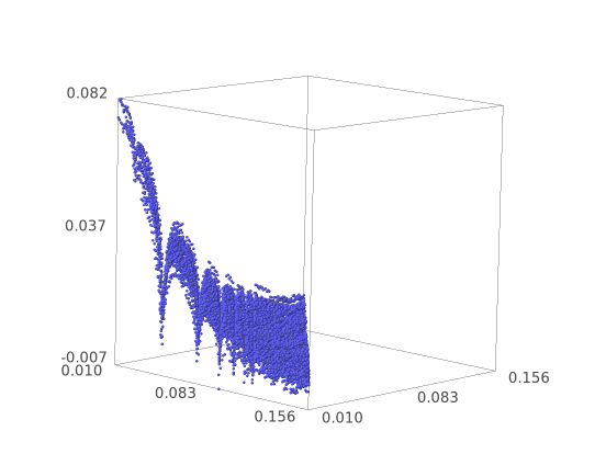
(a) side

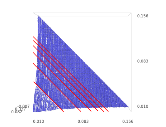
(b) top

We computed that for $x+y=25/3,50/9\text{ or }1/10$ the formula holds.

References

- [BH89] F. Beukers and G. Heckman. Monodromy for the hypergeometric function . Invent. Math., 95(2):325–354, 1989.
- [BM10] Irene I. Bouw and Martin Möller. Teichmüller curves, triangle groups, and Lyapunov exponents. Ann. of Math. (2), 172(1):139–185, 2010.
- [BT14] Christopher Brav and Hugh Thomas. Thin monodromy in Sp(4). Compos. Math., 150(3):333–343, 2014.
- [Dal07] Françoise Dal’Bo. Trajectoires géodésiques et horocycliques. Savoirs Actuels (Les Ulis). [Current Scholarship (Les Ulis)]. EDP Sciences, Les Ulis; CNRS Éditions, Paris, 2007.
- [DS13] Michael Dettweiler and Claude Sabbah. Hodge theory of the middle convolution. Publ. Res. Inst. Math. Sci., 49(4):761–800, 2013.
- [EKMZ16] Alex Eskin, Maxim Kontsevich, Martin Moeller, and Anton Zorich. Lower bounds for lyapunov exponents of flat bundles on curves, 2016.
- [EKZ14] Alex Eskin, Maxim Kontsevich, and Anton Zorich. Sum of Lyapunov exponents of the Hodge bundle with respect to the Teichmüller geodesic flow. Publ. Math. Inst. Hautes Études Sci., 120:207–333, 2014.
- [ES08] Christian Van Enckevort and Duco Van Straten. Monodromy calculations of fourth order equations of calabi–yau type. In in “Mirror Symmetry V”, the BIRS Proc. on Calabi–Yau Varieties and Mirror Symmetry, AMS/IP, 2008.
- [Fed15] Roman Fedorov. Variations of hodge structures for hypergeometric differential operators and parabolic higgs bundles, 2015.
- [Fil14] Simion Filip. Families of k3 surfaces and lyapunov exponents, 2014.
- [FMZ14] Giovanni Forni, Carlos Matheus, and Anton Zorich. Zero Lyapunov exponents of the Hodge bundle. Comment. Math. Helv., 89(2):489–535, 2014.
- [Kat96] Nicholas M. Katz. Rigid local systems, volume 139 of Annals of Mathematics Studies. Princeton University Press, Princeton, NJ, 1996.
- [KM16] André Kappes and Martin Möller. Lyapunov spectrum of ball quotients with applications to commensurability questions. Duke Math. J., 165(1):1–66, 2016.
- [Kon97] M. Kontsevich. Lyapunov exponents and Hodge theory. In The mathematical beauty of physics (Saclay, 1996), volume 24 of Adv. Ser. Math. Phys., pages 318–332. World Sci. Publ., River Edge, NJ, 1997.
- [Kri04] Raphaël Krikorian. Déviations de moyennes ergodiques, flots de teichmüller et cocycle de kontsevich-zorich. Séminaire Bourbaki, 46:59–94, 2003-2004.
- [Ser85] Caroline Series. The modular surface and continued fractions. J. London Math. Soc. (2), 31(1):69–80, 1985.
- [Sim90] Carlos T. Simpson. Harmonic bundles on noncompact curves. J. Amer. Math. Soc., 3(3):713–770, 1990.
- [SV14] Sandip Singh and T. N. Venkataramana. Arithmeticity of certain symplectic hypergeometric groups. Duke Math. J., 163(3):591–617, 2014.
- [Yos97] Masaaki Yoshida. Hypergeometric functions, my love. Aspects of Mathematics, E32. Friedr. Vieweg & Sohn, Braunschweig, 1997. Modular interpretations of configuration spaces.