The relationship between $k$-forcing and $k$-power domination

Abstract

Zero forcing and power domination are iterative processes on graphs where an initial set of vertices are observed, and additional vertices become observed based on some rules. In both cases, the goal is to eventually observe the entire graph using the fewest number of initial vertices. Chang et al. introduced $k$-power domination in [Generalized power domination in graphs, Discrete Applied Math. 160 (2012) 1691-1698] as a generalization of power domination and standard graph domination. Independently, Amos et al. defined $k$-forcing in [Upper bounds on the $k$-forcing number of a graph, Discrete Applied Math. 181 (2015) 1-10] to generalize zero forcing. In this paper, we combine the study of $k$-forcing and $k$-power domination, providing a new approach to analyze both processes. We give a relationship between the $k$-forcing and the $k$-power domination numbers of a graph that bounds one in terms of the other. We also obtain results using the contraction of subgraphs that allow the parallel computation of $k$-forcing and $k$-power dominating sets.

Keywords $k$-power domination, $k$-forcing, subgraph contraction, Sierpiński graphs

AMS subject classification 05C69, 05C50

1 Introduction

Zero forcing was introduced as a process to obtain an upper bound for the maximum nullity of real symmetric matrices whose nonzero pattern of off-diagonal entries is described by a given graph [2]. The minimum rank problem was motivated by the inverse eigenvalue problem of a graph. Independently, zero forcing was introduced by mathematical physicists studying quantum systems [5]. Since its introduction, zero forcing has attracted the attention of a large number of researchers who find the concept useful to model processes in a broad range of disciplines. The need for a uniform framework for the analysis of the diverse processes where the notion of zero forcing appears led to the introduction of a generalization of zero forcing called $k$-forcing [3].

Amos et al. proposed $k$-forcing in [3] as the following graph coloring game. Assume the vertices of a graph are colored in two colors, say white and blue. Iteratively apply the following color change rule: if $u$ is a blue vertex with at most $k$ white neighbors, then change the color of all the neighbors of $u$ to blue. Once this rule does not change the color of any vertex, if all vertices are blue, the original set of blue vertices is a $k$-forcing set of $G$. The original zero forcing is $1$-forcing under this definition. Because the problem of deciding whether a graph admits a $1$-forcing set of a given maximum size is NP-complete even if restricted to planar graphs [1, Theorem 2.3.1], the general problem of finding forcing sets cannot be solved algorithmically for large graphs without the development of further theoretical tools.

Power domination was introduced by Haynes et al. in [9] when using graph models to study the monitoring process of electrical power networks. When a power network is modeled by a graph, a power dominating set provides the locations where monitoring devices (Phase Measurement Units, or PMUs for short) can be placed in order to monitor the power network. Finding optimal PMU placements is an important practical problem in electrical engineering due to the cost of PMUs and network size. Although power domination is substantially different from standard graph domination, the notion of $k$-power domination was proposed as a generalization of both power domination ($k=1$) and standard graph domination ($k=0$) [6].

Chang et al. defined $k$-power domination in [6] using sets of observed vertices. Given a graph $G$ and a set of vertices $S$, initially all vertices in $S$ and their neighbors are observed; all other vertices are unobserved. Iteratively apply the following propagation rule: if there exists an observed vertex $u$ that has $k$ or fewer unobserved neighbors, then all the neighbors of $u$ are observed. Once this rule does not produce any additional observed vertices, if all vertices of $G$ are observed, $S$ is a $k$-power dominating set of $G$. Many problems outside graph theory can be formulated in terms of minimum $k$-power dominating sets [6] so methods to obtain them are highly desired. An algorithmic approach has been attempted, but the problem of deciding if a graphs admits a $k$-power dominating set of a given maximum size is NP-complete [6].

Although $k$-forcing and $k$-power domination have been studied independently, an in-depth analysis of $k$-power domination leads to the study of $k$-forcing. Indeed, after the initial step in which a set observes itself and its neighbors, the observation process in $k$-power domination proceeds exactly as the color changing process in $k$-forcing. The aim of this paper is to establish a precise connection between $k$-forcing and $k$-power domination to facilitate the transference of results, proofs, and methods between them, and ultimately to advance research on both problems.

Throughout this paper we work on $k$-forcing and $k$-power domination concurrently, using results in one process as stepping stones for results in the other one. In Section 2 we present the definitions and notation that we use in the rest of the paper. In Section 3 we give some core results and remarks that we use in the sections that follow.

In Section 4 we examine the effect of subgraph contraction in $k$-power domination and $k$-forcing. We obtain upper and lower bounds for the change in the $k$-power domination number produced by the contraction of a subgraph. Note that the contraction of a subgraph can increase or decrease its $k$-power domination number. In particular, we prove that the contraction of subgraphs of small degree can change the $k$-power domination number by at most one. In this section we also propose a way to decompose a graph in order to bound its $k$-power domination number in terms of that of smaller subgraphs. This can allow computation of $k$-power dominating sets to run in parallel. We also give the analogous results for $k$-forcing.

In Section 5 we present a lower bound for the $k$-power domination number of a graph in terms of its $k$-forcing number. This bound generalizes a known result for $k=1$ that gives the only lower bound for the power domination number of an arbitrary graph available so far [4]. As an application, we find an upper bound for the $k$-forcing number of a graph in terms of its maximum degree.

2 Definitions and notation

A graph is an ordered pair $G=(V,E)$ where $V=V(G)$ is a finite nonempty set of vertices and $E=E(G)$ is a set of unordered pairs of distinct vertices called edges (i.e., in this work graphs are simple and undirected). The order of $G$ is $|G|:=|V(G)|$. Two vertices $u$ and $v$ are adjacent or neighbors in $G$ if $\{u,v\}\in E(G)$. The (open) neighborhood of a vertex $v$ is the set $N_{G}(v)=\{u\in V:\{u,v\}\in E\}$, and the closed neighborhood of $v$ is the set $N_{G}[v]=N_{G}(v)\cup\{v\}$. Similarly, for any set of vertices $S$, $N_{G}(S)=\cup_{v\in S}N_{G}(v)$ and $N_{G}[S]=\cup_{v\in S}N_{G}[v]$. The degree of a vertex $v$ is $\deg_{G}(v):=|N(v)|$. The maximum and minimum degree of $G$ are $\Delta(G):=\max\{\deg_{G}(v):v\in V\}$ and $\delta(G):=\min\{\deg_{G}(v):v\in V\}$, respectively; a graph $G$ is regular if $\delta(G)=\Delta(G)$. We will omit the subscript $G$ when the graph $G$ is clear from the context.

A path joining $u,v\in V$ is a sequence of vertices $u=x_{0},x_{1},\ldots,x_{r}=v$ such that $\{x_{i},x_{i+1}\}\in E$ for each $i=0,\ldots,r-1$. A graph $G$ is connected if there is a path joining every pair of different vertices. If a graph is not connected, each maximal connected subgraph is a component of $G$. In this paper, $c(G)$ denotes the number of components of $G$ and $G_{1},\ldots,G_{c(G)}$ denote the components of $G$. Most of the results in this work are given for connected graphs, since if a graph is not connected, we can apply the results to each component.

If $X$ is a set of vertices of $G$, the subgraph induced by $X$ (in $G$) is denoted as $G[X]$; it has vertex set $X$ and edge set $\{\{u,v\}\in E:u,v\in X\}$. The graph $G-X$ is defined as $G[V\setminus X]$. The contraction of $X$ in $G$ is the graph $G/X$ obtained by adding a vertex $v_{X}$ to $G-X$ with $N_{G/X}(v_{X})=N_{G}[X]\setminus X$. Note that $G/X$ does not require $G[X]$ to be connected whereas the standard use of graph contraction does.

In a graph $G=(V,E)$, consider an arbitrary coloring of its vertices in two colors, say blue and white, and let $T$ denote the set of blue vertices. The color changing process in $k$-forcing can be formally described by associating to $T$ the family of sets $({\mathscr{F}}_{G,k}^{i}(T))_{i\geq 0}$ recursively defined by the following rules.

• ${\mathscr{F}}_{G,k}^{0}(T)=T$,

• ${\mathscr{F}}_{G,k}^{i+1}(T)={\mathscr{F}}_{G,k}^{i}(T)\cup\{N(v):v\in{\mathscr{F}}_{G,k}^{i}(T)\mbox{ and }1\leq|N_{G}(v)\setminus{\mathscr{F}}_{G,k}^{i}(T)|\leq k\}$, for $i\geq 0$.

A set $T\subseteq V$ is a $k$-forcing set of $G$ if there is an integer $t$ such that ${\mathscr{F}}_{G,k}^{t}(T)=V$. A minimum $k$-forcing set is a $k$-forcing set of minimum cardinality. The $k$-forcing number of $G$ is the cardinality of a minimum $k$-forcing set and is denoted by $Z_{k}(G)$. If $v\in{\mathscr{F}}_{G,k}^{i}(T)$ and $|N(v)\setminus{\mathscr{F}}_{G,k}^{i}(T)|\leq k$ then $v$ is said to $k$-force (or simply force if $k$ is clear from the context) every vertex in $N(v)\setminus{\mathscr{F}}_{G,k}^{i}(T)$.

Let $k$ be a nonnegative integer. The definition of $k$-power domination on a graph $G$ will be given in terms of a family of sets, $({\mathscr{P}}_{G,k}^{i}(S))_{i\geq 0}$, associated to each set of vertices $S$ in $G$.

• ${\mathscr{P}}_{G,k}^{0}(S)=N[S]$,

• ${\mathscr{P}}_{G,k}^{i+1}(S)={\mathscr{P}}_{G,k}^{i}(S)\cup\{N(v):v\in{\mathscr{P}}_{G,k}^{i}(S)\mbox{ and }1\leq|N_{G}(v)\setminus{\mathscr{P}}_{G,k}^{i}(S)|\leq k\}$, for $i\geq 0$.

A set $S\subseteq V$ is a $k$-power dominating set of $G$ if there is an integer $\ell$ such that ${\mathscr{P}}_{G,k}^{\ell}(S)=V$. A minimum $k$-power dominating set is a $k$-power dominating set of minimum cardinality. The $k$-power domination number of $G$ is the cardinality of a minimum $k$-power dominating set and is denoted by $\gamma_{P,k}(G)$.

Next we recall the definition of standard graph domination. A vertex $v$ dominates all vertices in $N_{G}[v]$. A set $S\subseteq V$ is a dominating set of $G$ if $N_{G}[S]=V$. The minimum cardinality of a dominating set is the domination number of $G$, denoted by $\gamma(G)$.

Note that $1$-forcing coincides with zero forcing [3], while $1$-power domination is exactly power domination and $0$-power domination coincides with domination [6].

3 Preliminaries

The following observations follow directly from the definitions of $k$-power domination and $k$-forcing, and provide the initial connection between both concepts.

Observation 3.1.

In any graph $G$, if $T$ is a $k$-forcing set, all sets $({\mathscr{F}}_{G,k}^{i}(T))_{i\geq 0}$ are $k$-forcing sets of $G$; if $S$ is a $k$-power dominating of $G$, the sets $({\mathscr{P}}_{G,k}^{i}(S))_{i\geq 0}$ are also $k$-forcing sets of $G$.

Observation 3.2.

In any graph $G$, if $T$ is a $k$-forcing set of $G$ then $T$ is also a $k$-power dominating set. The converse is not necessarily true, but $S$ is a $k$-power dominating set if and only if $N[S]$ is a $k$-forcing set. As a consequence, $\gamma_{P,k}(G)\leq Z_{k}(G)\leq\gamma_{P,k}(G)(\Delta(G)+1)$.

Observation 3.3.

In a graph $G$, $S\subsetneq V(G)$ is a $k$-power dominating set of $G$ if and only if $N[S]\setminus S$ is a $k$-forcing set of $G-S$.

Note that given a graph $G=(V,E)$ and $S\subseteq X\subseteq V$, it is possible that for some $x\in X$, $\deg_{G[X]}(x)<\deg_{G}(x)$. Therefore, the $k$-power domination process starting with $S$ in $G$ is different from the one starting with $S$ in $G[X]$. As a consequence, $S$ being a $k$-power dominating set of $G[X]$ does not imply that $S$ can $k$-observe all vertices in $X$ when propagating in $G$. Analogously, if $T\subseteq X\subseteq V$ then $T$ being a $k$-forcing set of $G[X]$ does not imply that $T$ can $k$-force $X$ in $G$. This observation motivates the following definitions.

Definition 3.4.

Let $G=(V,E)$ be a graph and let $A\subseteq X\subseteq V$. We say that $A$ is a $k$-forcing set of $X$ in $G$ if there exists a nonnegative integer $t$ such that $X\subseteq{\mathscr{F}}^{t}_{G,k}(A)$.

Definition 3.5.

Let $G=(V,E)$ be a graph and let $A\subseteq X\subseteq V$. We say that $A$ is a $k$-power dominating set of $X$ in $G$ if there exists a nonnegative integer $\ell$ such that $X\subseteq{\mathscr{P}}^{\ell}_{G,k}(A)$.

The proofs of the next results are straightforward, and are omitted.

Lemma 3.6.

Let $T$ be a $k$-forcing set of a graph $G$. Let $A\subseteq T$.

• If $A$ is $k$-forcing set of $T$ in $G$, then $A$ is a $k$-forcing set of $G$;

• If $A$ is $k$-power dominating set of $T$ in $G$, then $A$ is a $k$-power dominating set of $G$.

Lemma 3.7.

Let $S$ be a $k$-power dominating set of a graph $G$. Let $A\subseteq S$.

• If $A$ is $k$-forcing set of $N[S]$ in $G$, then $A$ is a $k$-forcing set of $G$;

• If $A$ is $k$-power dominating set of $N[S]$ in $G$, then $A$ is a $k$-power dominating set of $G$.

Lemma 3.8.

Let $G=(V,E)$ be a graph and $X\subseteq V$ such that $G[X]$ is connected and $\deg_{G}(x)\leq k+1$ for every $x\in X$. Let $u$ be an arbitrary vertex in $X$. Then $\{u\}$ is a (minimum) $k$-power dominating set of $N[X]$ in $G$. In addition, if $\deg_{G}(u)\leq k$, then $\{u\}$ is also a (minimum) $k$-forcing set of $N[X]$ in $G$.

Proof.

If $S=\{u\}$, then ${\mathscr{P}}_{G,k}^{0}(S)=N[u]$ and ${\mathscr{F}}_{G,k}^{0}(S)=\{u\}$. Since $\deg_{G}(x)\leq k+1$ for every $x\in X$, $x\neq u$ has at most $k$ unobserved neighbors when $x$ is observed. Thus, ${\mathscr{P}}_{G,k}^{i}(S)=N[{\mathscr{P}}_{G,k}^{i-1}(S)]$ for every integer $i\geq 1$. Since $G[X]$ is connected, there exists an integer $r\geq 1$ such that $X\subseteq{\mathscr{P}}_{G,k}^{r}(S)$. Once all vertices in $X$ are observed, each of them can have at most $k$ unobserved neighbors, so such a vertex can observe any unobserved neighbors. Thus, $N[X]\subseteq{\mathscr{P}}_{G,k}^{r+1}(S)$ and $S$ is a $k$-power dominating set of $N[X]$ in $G$. Now suppose $\deg_{G}(u)\leq k$. Then ${\mathscr{F}}_{G,k}^{1}(S)=N[S]$ and the argument proceeds as before. ∎

The following result follows immediately from Lemma 3.8, but is already known for $k$-power domination [6, Lemma 7]; a slightly weaker version for $k$-forcing is given in [3, Proposition 2.3].

Corollary 3.9.

Let $G$ be a connected graph. If $\Delta(G)\leq k+1$, then $\gamma_{P,k}(G)=1$; if in addition $\delta(G)\leq k$, then $Z_{k}(G)=1$.

When $G[X]$ is not connected, we apply Lemma 3.8 in each of its components and obtain the following result.

Corollary 3.10.

Let $G=(V,E)$ be a connected graph, $X\subseteq V$ and $u_{j}\in V(G[X]_{j})$ for every $j=1,\ldots,c(G[X])$. Let $S=\{u_{1},\ldots,u_{c(G[X])}\}$. If $\deg_{G}(x)\leq k+1$ for every $x\in X$, then $S$ is a minimum $k$-power dominating set of $N[X]$ in $G$; if in addition $\deg_{G}(u_{j})\leq k$ for every $j=1,\ldots,c(G[X])$, then $S$ is a minimum $k$-forcing set of $N[X]$ in $G$.

Proof.

By Lemma 3.8, for every $j=1,\ldots,c(G[X])$, $\{u_{j}\}$ is a $k$-power dominating set of $G[X]_{j}$ in $G$. Thus, $S$ is a $k$-power dominating set of $N[X]$ in $G$. Since every $k$-power dominating set of $N[X]$ must have at least one vertex in each component of $G[X]$ and $|S|=c(G[X])$ we conclude that $S$ is a minimum $k$-power dominating set of $N[X]$ in $G$. The argument for $k$-forcing is analogous. ∎

Lemma 3.11.

Let $G=(V_{G},E_{G})$ and $H=(V_{H},E_{H})$ be two graphs. Let $A\subseteq V_{G}$ and $B\subseteq V_{H}$ such that (i) $G-A=H-B$ and (ii) $N_{G}[A]\setminus A=N_{H}[B]\setminus B$. Then

• $A$ is a $k$-power dominating set of $G$ if and only if $B$ is a $k$-power dominating set of $H$;

• $N_{G}[A]$ is a $k$-forcing set of $G$ if and only if $N_{H}[B]$ is a $k$-forcing set of $H$.

Proof.

1) If $A$ is a $k$-power dominating set of $G$, then $N_{G}[A]\setminus A$ is a $k$-forcing set of $G-A$ by Observation 3.3. Since $G-A=H-B$ and $N_{G}[A]\setminus A=N_{H}[B]\setminus B$, we substitute $N_{G}[A]\setminus A$ and $G-A$ with $N_{H}[B]\setminus B$ and $H-B$, respectively, and obtain that $N_{H}[B]\setminus B$ is a $k$-forcing set of $H-B$. By Observation 3.3, $B$ is a $k$-power dominating set of $H$.

2) If $N_{G}[A]$ is a $k$-forcing set of $G$, then $A$ is a $k$-power dominating set of $G$ by Observation 3.2. Using 1) we conclude that $B$ is a $k$-power dominating set of $H$, and by Observation 3.2 we conclude that $N_{H}[B]$ is a $k$-forcing set of $H$. ∎

Corollary 3.12.

Let $G=(V_{G},E_{G})$ and $H=(V_{H},E_{H})$ be two graphs. Let $A\subseteq V_{G}$ and $B\subseteq V_{H}$ such that (i) $G-A=H-B$ and (ii) $N_{G}[A]\setminus A=N_{H}[B]\setminus B$. Let $P\subseteq V_{G}\setminus A=V_{H}\setminus B$. Then

• $A\cup P$ is a $k$-power dominating set of $G$ if and only if $B\cup P$ is a $k$-power dominating set of $H$;

• $N_{G}[A]\cup P$ is a $k$-forcing set of $G$ if and only if $N_{G}[B]\cup P$ is a $k$-forcing set of $H$.

Proof.

Define $A^{\prime}=A\cup P$ and $B^{\prime}=B\cup P$. Then $G-A^{\prime}=H-B^{\prime}$ and $N_{G}[A^{\prime}]\setminus A^{\prime}=N_{H}[B^{\prime}]\setminus B^{\prime}$, so we can apply Lemma 3.11 with $G$, $H$, $A^{\prime}$ and $B^{\prime}$. ∎

While all the previous results include analogous statements for $k$-forcing and a $k$-power domination, the following lemma does not have a $k$-forcing analog.

Lemma 3.13.

[6, Lemma 9] If $G$ is connected and $\Delta(G)\geq k+2$, then there exists a minimum $k$-power dominating set $S$ such that $\deg(v)\geq k+2$ for all $v\in S$.

To see that there is no $k$-forcing analog to Lemma 3.13 it is sufficient to consider $K_{1,n}$, the complete bipartite graph with one vertex in one part and $n$ vertices in the other. As shown in [3], if $n>k$ every minimum $k$-forcing set contains at least one vertex of degree $1$.

4 Graph contraction

Definition 4.1.

Let $G$ be a graph and let $X\subseteq V(G)$. Define $\widehat{X}$ to be the graph obtained from $G[X]$ by attaching to each one of its vertices as many pendent vertices as its number of neighbors in $G-X$.

Lemma 4.2.

Let $G$ be a connected graph and let $X\subseteq V(G)$. There exists $S\subseteq X$ such that $S$ is a minimum $k$-power dominating set of $\widehat{X}$.

Proof.

Suppose first that $\Delta(\widehat{X})\leq k+1$. Then by Lemma 3.8 any one vertex of $X$ is a $k$-power dominating set for $N[X]=\widehat{X}$; a one vertex $k$-power dominating set is necessarily minimum. Now assume $\Delta(\widehat{X})\geq k+2$. By definition of $\widehat{X}$, $\deg_{\widehat{X}}(u)=1$ for every $u\in V(\widehat{X})\setminus X$. Since $\Delta(\widehat{X})\geq k+2$, by Lemma 3.13 there exists a minimum $k$-power dominating set $S$ of $\widehat{X}$ that contains only vertices in $X$. ∎

For the same reasons why there is no $k$-forcing analog to Lemma 3.13, there is no $k$-forcing analog to Lemma 4.2. Indeed, if $x\in V(G)$ and $\deg_{G}(x)\geq k+1$, a minimum $k$-forcing set of $\widehat{\{x\}}$ must contain a vertex of degree 1.

Lemma 4.3.

Let $G$ be a connected graph and let $X\subseteq V(G)$. If $S\subseteq X$ is a minimum $k$-power dominating set of $\widehat{X}$, then $S$ is a $k$-power dominating set of $N_{G}[X]$ in $G$.

Proof.

Each vertex in $V(\widehat{X})\setminus X$ arises from a vertex $y\notin X$ that is a neighbor of a vertex $x\in X$. For every $x\in X$, let $N_{x}$ denote the (possibly empty) set of neighbors of $x$ in $V(\widehat{X})\setminus X$ (i.e., $N_{x}=N_{\widehat{X}}(x)\setminus X$) and let $N^{\prime}_{x}=N_{G}(x)\setminus X$. Since $S\subseteq X$ and $\deg_{\widehat{X}}(u)=1$ for every $u\in V(\widehat{X})\setminus X$, none of the vertices in $N_{x}$ can be observed before $x$ is observed, and moreover, all vertices in $N_{x}$ are observed simultaneously. Since for every $x\in V(\widehat{X})$, $\deg_{\widehat{X}}(x)=\deg_{G}(x)$, the only difference between the $k$-power domination process starting with $S$ in $\widehat{X}$ and the one starting with $S$ in $G$ is that when the vertices in $N_{x}$ are observed in $\widehat{X}$, the unobserved vertices in $N^{\prime}_{x}$ become observed in $G$. The reason why some vertices in $N^{\prime}_{x}$ could have been observed earlier is that a vertex in $G-X$ could have more than one neighbor in $X$ so $(N^{\prime}_{x})_{x\in X}$ are not necessarily disjoint. Since for every $w\in N_{G}[X]\setminus X$ there exists $x\in X$ such that $w\in N^{\prime}_{x}$, all vertices in $N_{G}[X]$ are observed. ∎

Theorem 4.4.

Let $G=(V,E)$ be a connected graph. If $X\subseteq V$,

$$\gamma_{P,k}(G/X)-1\leq\gamma_{P,k}(G)\leq\gamma_{P,k}(G/X)+\gamma_{P,k}(\widehat{X})$$

and both bounds are tight.

Proof.

Let $H=G/X$. By Lemma 4.2 there exists $\widehat{P}\subseteq X$ such that $\widehat{P}$ is a minimum $k$-power dominating set of $\widehat{X}$ and by Lemma 4.3, $\widehat{P}$ is also a $k$-power dominating set of $N_{G}[X]$ in $G$.

To prove the upper bound we show that if $P$ is a $k$-power dominating set of $H$, then $(P\setminus\{v_{X}\})\cup\widehat{P}$ is a $k$-power dominating set of $G$. Since $\widehat{P}$ is a $k$-power dominating set of $N_{G}[X]$ in $G$, clearly $(P\setminus\{v_{X}\})\cup\widehat{P}$ is a $k$-power dominating set of $N_{G}[P\setminus\{v_{X}\}]\cup N_{G}[X]=N_{G}[P\setminus\{v_{X}\}\cup X]$ in $G$. We will prove that $(P\setminus\{v_{X}\})\cup X$ is a $k$-power dominating set of $G$, which by Lemma 3.7 suffices to conclude that $(P\setminus\{v_{X}\})\cup\widehat{P}$ is a $k$-power dominating set of $G$. Let $A=X$ and $B=\{v_{X}\}$. Since $H=G/X$, $G-A=H-B$ and $N_{G}[A]\setminus A=N_{H}[B]\setminus B$, we apply Corollary 3.12 and conclude that $(P\setminus\{v_{X}\})\cup A$ is a $k$-power dominating set of $G$ if and only if $(P\setminus\{v_{X}\})\cup B$ is a $k$-power dominating set of $H$. Since $B=\{v_{X}\}$, $(P\setminus\{v_{X}\})\cup B=P$ and $P$ is a $k$-power dominating set of $H$, $(P\setminus\{v_{X}\})\cup A=(P\setminus\{v_{X}\})\cup X$ is a $k$-power dominating set of $G$.

To prove the lower bound, we show that if $S$ is a minimum $k$-power dominating set of $G$, then $(S\setminus X)\cup\{v_{X}\}$ is a $k$-power dominating set of $H$. As above, let $A=X$ and $B=\{v_{X}\}$ so $G-A=H-B$ and $N_{G}[A]\setminus A=N_{H}[B]\setminus B$. Then we apply Corollary 3.12 to conclude that $(S\setminus X)\cup A$ is a $k$-power dominating set of $G$ if and only if $(S\setminus X)\cup B$ is a $k$-power dominating set of $H$. Since $X=A$, then $(S\setminus X)\cup A=S$ and it is a $k$-power dominating set of $G$. Then $(S\setminus X)\cup B=(S\setminus X)\cup\{v_{X}\}$ is a $k$-power dominating set of $H$. Thus, $\gamma_{P,k}(G/X)\leq|(S\setminus X)\cup\{v_{X}\}|\leq|S|+1=\gamma_{P,k}(G)+1$.

To prove the upper bound is tight, for each integer $q\geq k$ we define a graph $U_{q}$ and a set $X\subseteq V(U_{q})$ such that $\gamma_{P,k}(U_{q})=\gamma_{P,k}(U_{q}/X)+\gamma_{P,k}(\widehat{X})$ (see Figure 1). Consider two disjoint copies of $K_{q+2}$, say $G$ and $G^{\prime}$, and vertices $x\in V(G)$ and $y\in V(G^{\prime})$. Construct $U_{q}$ by adding the edge $e=\{x,y\}$ and define $X=V(G^{\prime})\setminus\{y\}$. Then $\gamma_{P,k}({U_{q}})=2$, $\gamma_{P,k}(\widehat{X})=1$, and $\gamma_{P,k}(U_{q}/X)=1$.

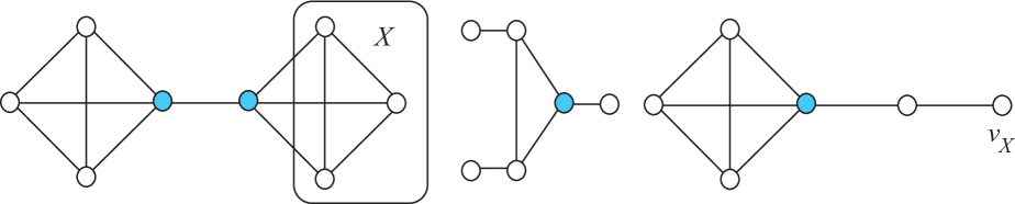
$U_{2}$          $\widehat{X}$         $U_{2}/X$

Figure 1: The graphs $U_{2}$, $\widehat{X}$, and $U_{2}/X$ defined in Theorem 4.4 are shown. In each case, a minimum $2$-power dominating set is indicated by coloring.

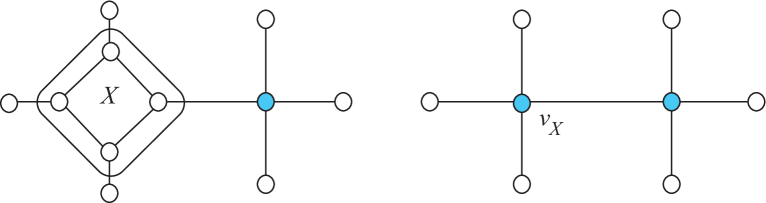
$L_{2}$          $L_{2}/X$

Figure 2: The graphs $L_{2}$ and $L_{2}/X$ defined in Theorem 4.4 are shown. In each case, a minimum $2$-power dominating set is indicated by coloring.

To show the lower bound is tight, for each integer $q\geq k$ we define a graph $L_{q}$ and a set $X\subseteq V(L_{q})$ such that $\gamma_{P,k}(L_{q}/X)-1=\gamma_{P,k}(L_{q})$ (see Figure 2). Assume first that $k\geq 2$. Construct $L_{q}$ starting with a cycle of length $2q$ with vertices $v_{1},\ldots,v_{2q}$. Attach a pendent vertex to each vertex $v_{i}$, for $i=1,\ldots,2q$. Then attach $q+1$ pendent vertices to the pendent neighbor of $v_{1}$, so $\gamma_{P,k}(L_{q})=1$. For $X=\{v_{1},\ldots,v_{2p}\}$, $\gamma_{P,k}(L_{q}/X)=2$. Now suppose $k=1$, and begin with a path of length $6$ with vertices $v_{0},\ldots,v_{6}$. Construct $L_{q}$ by attaching $q$ pendent vertices to $v_{0}$. If $X=\{v_{1},v_{3},v_{5}\}$, then $\gamma_{P,1}(L_{q})=1$ and $\gamma_{P,1}(L_{q}/X)=2$. ∎

The next example shows that it is possible to find a graph $G$ and a subgraph $X$ for which the gap between $\gamma_{P,k}(G)$ and $\gamma_{P,k}(G/X)$ is arbitrarily large.

Example 4.5.

Given a positive integer $c$, define $T_{k,c}$ as the tree obtained by adding $k+2$ leaves to each leaf of $K_{1,c}$. If $X$ is the set of all vertices of degree greater than one in $T_{k,c}$, then $\gamma_{P,k}(T_{k,c})=\gamma_{P,k}(\widehat{X})=c$ and $\gamma_{P,k}(T_{k,c}/X)=1$.

Corollary 4.6.

Let $G=(V,E)$ be a connected graph. Let $X\subseteq V$ such that $\deg_{G}(x)\leq k+1$ for every $x\in X$. Then

$$\gamma_{P,k}(G/X)-1\leq\gamma_{P,k}(G)\leq\gamma_{P,k}(G/X)+c(G[X]).$$

Proof.

It is sufficient to show that $\gamma_{P,k}(\widehat{X})\leq c(G[X])$. Observe that $\deg_{G}(x)\leq k+1$ for every $x\in X$ implies that $\deg_{\widehat{X}}(x)\leq k+1$ for every $x\in V(\widehat{X})$. By Corollary 3.10 there exists a $k$-power dominating set of $N_{\widehat{X}}[X]=V(\widehat{X})$ in $G$ with cardinality $c(\widehat{X})=c(G[X])$, so $\gamma_{P,k}(\widehat{X})\leq c(G[X])$. ∎

Corollary 4.7.

Let $G=(V,E)$ be a connected graph. Let $X\subseteq V$ such that $G[X]$ is connected and $\deg_{G}(x)\leq k+1$ for every $x\in X$.Then

$$\gamma_{P,k}(G/X)-1\leq\gamma_{P,k}(G)\leq\gamma_{P,k}(G/X)+1.$$

Proposition 4.8.

Let $G=(V,E)$ be a connected graph. Let $X\subseteq V$ such that $G[X]$ is connected and $\deg_{G}(x)\leq 2$ for every $x\in X$. Then $\gamma_{P,1}(G/X)\leq\gamma_{P,1}(G)$ and this bound it tight.

Proof.

Since $\Delta(G)\leq 2$ implies that $G$ itself is a path or a cycle, without loss of generality we can assume $\Delta(G)\geq 3$. By Lemma 3.13, there exists a minimum $k$-power dominating set $S$ of $G$ such that $\deg_{G}(u)\geq 3$ for every $u\in S$, so $S\subseteq V\setminus X$. We prove that $S$ is also a $k$-power dominating set of $H$.

As in the proof of Theorem 4.4, $S\cup\{v_{X}\}$ is a $k$-power dominating set of $H$. Then by Observation 3.2, $N_{H}[S\cup\{v_{X}\}]=N_{H}[S]\cup N_{H}[v_{X}]$ is a $k$-forcing set of $H$.

Note that $S\subseteq V\setminus X$ implies ${\mathscr{P}}_{G,k}^{0}(S)\setminus X={\mathscr{P}}_{H,k}^{0}(S)\setminus\{v_{X}\}$ and as long as ${\mathscr{P}}_{G,k}^{i}(S)\subseteq V\setminus X$, ${\mathscr{P}}_{G,k}^{i}(S)={\mathscr{P}}_{H,k}^{i}(S)$. Let $x$ be a vertex of $X$ that is observed first (meaning that no vertex of $X$ has been observed earlier), and let $y$ be the vertex in $G-X$ that dominates or forces $x$ at time $t$ ($x\in{\mathscr{P}}_{G,k}^{0}(S)$ or $x\in{\mathscr{P}}_{G,k}^{t}(S)\setminus{\mathscr{P}}_{G,k}^{t-1}(S)$ for $t\geq 1$). Since $\deg_{G}(y)\geq\deg_{H}(y)$, $y$ can also dominate or force in $H$. Thus $v_{X}\in{\mathscr{P}}_{H,k}^{t}(S)$. Since $\deg_{H}(v_{X})\leq 2$, it takes at most one additional application of $k$-forcing to observe all vertices in $N_{H}[v_{X}]$, so $N_{H}[v_{X}]\subseteq{\mathscr{P}}_{H,k}^{t+1}(S)$.

Since $N_{H}[S]={\mathscr{P}}_{H,k}^{0}(S)\subseteq{\mathscr{P}}_{H,k}^{t+1}(S)$ and $N_{H}[v_{X}]\subseteq{\mathscr{P}}_{H,k}^{t+1}(S)$, then $N_{H}[S\cup\{v_{X}\}]=N_{H}[S]\cup N_{H}[v_{X}]\subseteq{\mathscr{P}}_{H,k}^{t+1}(S)$. Moreover, since $N_{H}[S\cup\{v_{X}\}]$ is a $k$-forcing set of $H$, so is ${\mathscr{P}}_{H,k}^{t+1}(S)$ and therefore, $S$ is a $k$-power dominating set of $H$.

To prove the tightness, observe that for $n\geq 3$, contracting the set of all vertices of degree $2$ in the path $P_{n}$ of order $n$ produces the path $P_{3}$. Now, $\gamma_{P,1}(P_{n})=\gamma_{P,1}(P_{3})=1$. ∎

Due to the computational complexity of the $k$-power domination problem, efficient algorithms to approximate of optimal $k$-power dominating sets are of practical importance. Theorem 4.4 could help in the parallel search for $k$-power dominating sets. The following result provides a theoretical framework to study practical uses of graph decomposition as a tool for the parallel computation of $k$-power dominating sets.

Theorem 4.9.

Let $G=(V,E)$ be a connected graph and let $P_{1},\ldots,P_{r}$ be a partition of $V$. Then

$$\gamma_{P,k}(G)\leq\sum_{i=1}^{r}\gamma_{P,k}(\widehat{P_{i}}).$$

Proof.

By Lemma 4.2, for every $i=1,\ldots,r$ there exists $S_{i}\subseteq P_{i}$ such that $S_{i}$ is a minimum $k$-power dominating set of $\widehat{P_{i}}$. By Lemma 4.3, $S_{i}$ is also a $k$-power dominating set of $N_{G}[P_{i}]$ in $G$, and as a consequence, $S=\cup_{i=1}^{r}S_{i}$ is a $k$-power dominating set of $G$. Then $\gamma_{P,k}(G)\leq|S|\leq\sum_{i=1}^{r}|S_{i}|=\sum_{i=1}^{r}\gamma_{P,k}(\widehat{P_{i}})$. ∎

To prove that the bound in Theorem 4.9 is tight we will use the family of Sierpiński graphs whose definition we recall, using the notation in [8]. Given two positive integers $n$ and $p$ the Sierpiński graph $S_{p}^{n}$ has as vertices all $n$-tuples of integers in $\{0,1,\ldots,p-1\}$ denoted as $s_{n}s_{n-1}\cdots s_{2}s_{1}$. Two vertices $s_{n}\cdots s_{1}$ and $t_{n}\cdots t_{1}$ are adjacent in $S_{p}^{n}$ if and only if there exists an $r$ with $1\leq r\leq n$ such that

• $s_{i}=t_{i}$ for every $i\in\{r+1,\ldots,n\}$,

• $s_{r}\not=t_{r}$, and

• $s_{i}=t_{r}$ and $t_{i}=s_{r}$ for every $i\in\{1,\ldots,r-1\}$

The definition of Sierpiński graphs implies that $S_{p}^{1}=K_{p}$ and if $n\geq 2$, $S_{p}^{n}$ has $p^{n-i}$ induced copies of $S_{p}^{i}$. Moreover, the vertices in each of those copies coincide in the $n-i$ leftmost digits $s_{n}\cdots s_{i+1}$ [8]. If $s$ is a $(n-i)$-tuple of integers in $\{0,\ldots,p-1\}$, let $sS_{p}^{i}$ denote the set of vertices of $S_{p}^{n}$ whose leftmost $n-i$ digits coincide with $s$. For simplicity, we use $S_{p}^{n}[s]$ to denote $S_{p}^{n}[sS_{p}^{i}]$ (the subgraph induced by $sS_{p}^{i}$ in $S_{p}^{n}$), so $S_{p}^{n}[s]$ is isomorphic to $S_{p}^{i}$.

Lemma 4.10.

Given integers $n\geq 4$, $k\geq 1$ and $p\geq k+2$, let $s$ be a $(n-3)$-tuple of integers in $\{0,\ldots,p-1\}$. Then $\gamma_{P,k}(\widehat{sS_{p}^{3}})=\gamma_{P,k}(S_{p}^{3})$.

Proof.

Fix $k\geq 1$, $p\geq k+2$, and $n\geq 4$. We begin by determining the degree of a vertex $sxyz$ in $S^{n}_{p}$ and in $S_{p}^{n}[s]\cong S_{p}^{3}$. The definition of the Sierpiński graph $S_{p}^{n}$ implies that vertices of the form $a^{n}$ have degree $p-1$ and all the other vertices have degree $p$ in $S_{p}^{n}$. If $xyz$ is nonconstant, then vertex $sxyz$ has degree $p$ in both $S_{p}^{n}$ and $S_{p}^{n}[s]$, so $sxyz$ does not have any pendent vertices added in $\widehat{sS_{p}^{3}}$. Now consider the constant sequence $aaa$. If $s\neq a^{n-3}$, then vertex $saaa$ has degree $p$ in $S_{p}^{n}$ but degree $p-1$ in $S_{p}^{n}[s]$, so one leaf is added to $saaa$ in $\widehat{sS_{p}^{3}}$. If $s=a^{n-3}$, then vertex $saaa=a^{n}$ has degree $p-1$ in both $S_{p}^{n}$ and $S_{p}^{n}[s]$, so $saaa$ is unchanged in $\widehat{sS_{p}^{3}}$.

If $s\neq a^{n-3}$ for any $a\in\{0,\ldots,p-1\}$, then $\widehat{sS_{p}^{3}}$ is obtained from $S_{p}^{n}[s]$ by attaching one pendent vertex to each of the $p$ vertices of the form $saaa$ for $a\in\{0,\ldots,p-1\}$, so that every vertex of $\widehat{sS_{p}^{3}}$ has degree $p$; denote this graph by $G_{1}$. If $s=a^{n-3}$ for some $a\in\{0,\ldots,p-1\}$, then $\widehat{sS_{p}^{3}}$ is obtained from $S_{p}^{n}[s]$ by attaching one pendent vertex to each of the $p-1$ vertices of the form $sbbb$ for $b\neq a$, so that every vertex of $\widehat{sS_{p}^{3}}$ except $a^{n}$ has degree $p$; denote this graph by $G_{2}$. Observe that the only difference between $G_{1}$ and $G_{2}$ is that $G_{2}$ is missing one leaf.

To show that $\gamma_{P,k}(G_{i})=\gamma_{P,k}({S_{p}^{3}})$ for $i=1,2$, we first we prove $\gamma_{P,k}(G_{i})\leq\gamma_{P,k}({S_{p}^{3}})$ by showing that if $P$ is a $k$-power dominating set of $S_{p}^{3}$, then $P$ is also a $k$-power dominating set of $G_{i}$. For each pendent vertex $x$ in $G_{i}$, let $u_{x}$ denote its only neighbor (in $G_{i}$). Then $u_{x}$ is a vertex of degree $p-1$ in $S_{p}^{3}$ and therefore, in $S_{p}^{3}$ it is labeled as $a^{3}$ for some $a\in\{0,\ldots,p-1\}$. If $u_{x}\in P$, then $x\in N_{G_{i}}[P]={{\mathscr{P}}_{{G_{i}},k}^{0}(P)}$. If $u_{x}\notin P$, then $u_{x}\in{{\mathscr{P}}_{{S_{p}^{3}},k}^{t}(P)}$ for some integer $t>0$. Note that in $S_{p}^{3}$, $u_{x}$ cannot be observed until one of its neighbors is. Since $u_{x}=a^{3}$, its $p-1$ neighbors in $S_{p}^{3}$ have labels in the form $aab$ for $b=0,\ldots,p-1$, $b\not=a$. Therefore, $N_{S_{p}^{3}}[u_{x}]$ induces a $p$-clique in $S_{p}^{3}$. This means that when a neighbor forces $u_{x}$, it also forces all the vertices in the $p$-clique induced by $N_{S_{p}^{3}}[u_{x}]$. When this happens in $G_{i}$ instead of in $S_{p}^{3}$, $u_{x}$ has exactly one unobserved neighbor ($x$), so $x\in{{\mathscr{P}}_{{S_{p}^{3}},k}^{t+1}(P)}$.

Finally we prove $\gamma_{P,k}(G_{i})\geq\gamma_{P,k}({S_{p}^{3}})$ by showing that there exists a minimum $k$-power dominating set $Q$ of $G_{i}$ that is also a $k$-power dominating set of $S_{p}^{3}$. By Lemma 3.13 there exists a minimum $k$-power dominating set $Q$ of $G_{i}$ that does not contain vertices of degree $1$, so $Q\subseteq V({S_{p}^{3}})$. Therefore, in the $k$-power domination process starting with $Q$ in $G_{i}$, a vertex of degree $1$ in $G_{i}$ cannot be observed until its one neighbor in $S_{p}^{3}$ is. Then $Q$ is a $k$-power dominating set of $S_{p}^{3}$. We conclude that $\gamma_{P,k}(\widehat{sS_{p}^{3}})=\gamma_{P,k}(S_{p}^{3})$. ∎

It is known that if $n\geq 3$, $k\geq 1$, and $p\geq k+2$, then $\gamma_{P,k}(S_{p}^{n})=p^{n-2}(p-k-1)$ [8] so we immediately obtain the following result.

Corollary 4.11.

Given integers $n\geq 4$, $k\geq 1,$ and $p\geq k+2$, let $s$ be a $(n-3)$-tuple of integers in $\{0,\ldots,p-1\}$. Then $\gamma_{P,k}(\widehat{sS_{p}^{3}})=p(p-k-1)$.

Lemma 4.12.

Given integers $n\geq 4$, $k\geq 1$, and $p\geq k+2$, let $T$ denote the set of all $(n-3)$-tuples of integers in $\{0,\ldots,p-1\}$. Then $\gamma_{P,k}(S_{p}^{n})=\sum_{t\in T}\gamma_{P,k}(\widehat{tS_{p}^{3}})$.

Proof.

By Lemma 4.11 $\gamma_{P,k}(\widehat{tS_{p}^{3}})=\gamma_{P,k}(S_{p}^{3})=p(p-k-1)$ for every $t\in T$. There are $p^{n-3}$ tuples in $T$, so $\sum_{t\in T}\gamma_{P,k}(\widehat{tS_{p}^{3}})=p^{n-3}p(p-k-1)=p^{n-2}(p-k-1)=\gamma_{P,k}(S_{p}^{n})=p^{n-2}(p-k-1)$. ∎

The bound in Theorem 4.9 is $\gamma_{P,k}(S_{p}^{n})\leq\sum_{t\in T}\gamma_{P,k}(\widehat{{tS_{p}^{3}}})$, so the following result is an immediate consequence of Lemma 4.12.

Corollary 4.13.

The bound in Theorem 4.9 is tight.

Next we present the equivalent results for $k$-forcing taking into consideration the following differences between $k$-power domination and $k$-forcing. The proofs are analogous and are omitted.

• For the lower bound, note that if $\deg_{H}(v_{X})>k$, $\{v_{X}\}$ does not force $N_{H}(v_{X})=N_{G}[X]\setminus X$. In that case, to obtain a $k$-forcing set of $H$ from a $k$-forcing set of $G$ it might be necessary to add at most $|N_{G}[X]\setminus X|-k$ vertices.

• For the upper bound, since there is no $k$-forcing equivalent to Lemma 4.2, it could happen that every minimum $k$-forcing set of $\widehat{X}$ contains a vertex $x\in N[X]\setminus X$ for which $\deg_{\widehat{X}}(x)=1$ but $\deg_{G}(x)>k$. Thus, $x$ forces its neighbors in $\widehat{X}$ but not in $G$, and a $k$-forcing set of $\widehat{X}$ might not force $X$ in $G$.

Proposition 4.14.

Let $G=(V,E)$ be a connected graph. Let $X\subseteq V(G)$. If there exists a minimum $k$-forcing set of $\widehat{X}$ that contains only vertices in $X$, then

$$Z_{k}(G/X)+Z_{k}(\widehat{X})\geq Z_{k}(G)\geq\left\{\begin{array}[]{ll}Z_{k}(G/X)-1&\mbox{ if }|N[X]\setminus X|\leq k,\\ Z_{k}(G/X)-|N[X]\setminus X|+k&\mbox{ if }|N[X]\setminus X|>k.\end{array}\right.$$

Proposition 4.15.

Let $G=(V,E)$ be a connected graph. Let $X\subseteq V$ such that $\deg_{G}(x)\leq k$ for $x\in X$. If there exists a minimum $k$-forcing set of $\widehat{X}$ that contains only vertices in $X$, then

$$Z_{k}(G/X)+c(G[X])\geq Z_{k}(G)\geq\left\{\begin{array}[]{ll}Z_{k}(G/X)-1&\mbox{ if }|N[X]\setminus X|\leq k,\\ Z_{k}(G/X)-|N[X]\setminus X|+k&\mbox{ if }|N[X]\setminus X|>k.\end{array}\right.$$

Corollary 4.16.

[10, Theorem 5.1] For any edge $e$ in a graph $G$, $Z(G)-1\leq Z(G/e)\leq Z(G)+1.$

Theorem 4.17.

Let $G=(V,E)$ be a connected graph and let $P_{1},\ldots,P_{r}$ be a partition of $V$. If $\widehat{P_{i}}$ has a minimum $k$-power dominating set in $P_{i}$ for every $i=1,\ldots,r$, then

$$\operatorname{Z}_{k}(G)\leq\sum_{i=1}^{r}\operatorname{Z}_{k}(\widehat{P_{i}}).$$

Theorem 4.9 and Theorem 4.17 provide upper bounds for the $k$-power domination and the $k$-forcing number of a graph in terms of the $k$-power domination and the $k$-forcing number of $\widehat{P_{1}},\ldots,\widehat{P_{r}}$, which can be computed in parallel. In particular, the importance of Theorems 4.9 and 4.17 resides in the fact that $\widehat{P}_{i}$ might have properties that do not hold for $G$. For example, suppose $G$ is not a tree, but there is a linear algorithm to partition $V(G)$ into sets $P_{1},\ldots,P_{r}$ such that $\widehat{P_{1}},\ldots,\widehat{P_{r}}$ are trees. Then using the linear algorithm for trees provided in [7], $\gamma_{P,k}(\widehat{X})$ can be computed in linear time. The exploration of possible uses of our results in algorithms to find $k$-power dominating or $k$-forcing sets a graph requires a detailed and careful analysis that is outside the scope of this paper.

5 $k$-power domination and $k$-forcing numbers

By Observation 3.2, $\gamma_{P,k}(G)\leq Z_{k}(G)\leq\gamma_{P,k}(G)(\Delta(G)+1).$ In this section we improve the upper bound in the previous inequality by generalizing a result by Benson et al. [4, Theorem 3.2] for 1-power domination. An important concept in this work is that of private neighborhood, which we recall. Suppose $v\in S\subseteq V$. A $S$-private neighbor of $v$ is a vertex $x\in N(v)$ such that $x\notin N(S\setminus\{v\})$. Moreover, we say that $x$ is an external $S$-private neighbor if $x\notin S$.

Lemma 5.1.

[6, Lemma 10] In every connected graph $G$ with $\Delta(G)\geq k+2$ there exists a minimum $k$-power dominating set $S$ in which every vertex has at least $k+1$ $S$-private neighbors.

We strengthen Lemma 5.1 by extending it to external private neighbors.

Lemma 5.2.

In every connected graph $G$ with $\Delta(G)\geq k+2$ there exists a minimum $k$-power dominating set $S$ in which every vertex has at least $k+1$ external $S$-private neighbors.

Proof.

By Lemma 5.1 there exists a minimum $k$-power dominating set $S$ in which every vertex has at least $k+1$ $S$-private neighbors. Suppose that there exists $u\in S$ that has at most $k$ external private neighbors. We prove that $S^{\prime}=S\setminus\{u\}$ is $k$-power dominating set, which contradicts the minimality of $S$. Since $u$ has at least $k+1$ neighbors and at most $k$ of them are outside $S$, there exists $y\in S$ such that $u$ and $y$ are neighbors. This implies that $u\in{{\mathscr{P}}_{G,k}}^{0}(S^{\prime})$. Moreover, all non-external neighbors of $u$ are in $S$ and thus in ${{\mathscr{P}}_{G,k}}^{0}(S^{\prime})$ so $u$ has at most $k$ unobserved neighbors. Thus, $N_{G}[u]\subseteq{{\mathscr{P}}_{G,k}}^{1}(S^{\prime})$, so $S^{\prime}$ is a $k$-power dominating set. ∎

Lemma 5.3.

If $G$ is a connected graph with $\Delta(G)\geq k+2$ and $S=\{u_{1},\dots,u_{t}\}$ is a minimum $k$-power dominating set of $G$ in which every vertex has at least $k+1$ external $S$-private neighbors, then

$$\operatorname{Z}_{k}(G)\leq\sum_{i=1}^{t}(\deg u_{i}+1-k).$$

Proof.

By hypothesis, for each $i=1,\ldots,t$ there exists a set $\{x_{1}^{(i)},\dots,x_{k}^{(i)}\}$ of external $S$-private neighbors of $u_{i}$. We prove that $B:=\bigcup_{i=1}^{t}\left(N[u_{i}]\setminus\{x_{1}^{(i)},\dots,x_{k}^{(i)}\}\right)$ is a $k$-forcing set of $G$. Since $x_{1}^{(i)},\dots,x_{k}^{(i)}$ are external $S$-private neighbors of $u_{i}$, then $\{x_{1}^{(i)},\dots,x_{k}^{(i)}\}\cap S=\emptyset$, which implies $u_{i}\in B$, for every $i=1,\ldots,t$. In the first step of the $k$-forcing process each vertex $u_{i}$ forces $x_{1}^{(i)},\dots,x_{k}^{(i)}$ so $B$ is a $k$-forcing set of $N[S]$ in $G$. Since $S$ is a $k$-power dominating set of $G$, by Observation 3.2 $N[S]$ is a $k$-forcing set of $G$. Then by Observation 3.6, $B$ is a $k$-forcing set of $G$ so, $\operatorname{Z}_{k}(G)\leq|B|\leq\sum_{i=1}^{t}\left|N[u_{i}]\setminus\{x_{1}^{(i)},\dots,x_{k}^{(i)}\}\right|\leq\sum_{i=1}^{t}(\deg u_{i}+1-k).$ ∎

Theorem 5.4.

In every connected graph $G$ with $\Delta(G)\geq k+2$,

$$\operatorname{Z}_{k}(G)\leq\gamma_{P,k}(G)({\Delta(G)+1-k}),\mbox{ or equivalently, }\left\lceil\frac{\operatorname{Z}_{k}(G)}{\Delta(G)+1-k}\right\rceil\leq\gamma_{P,k}(G)$$

and this lower bound for $\gamma_{P,k}(G)$ is tight.

Proof.

By Lemma 5.2 there exists a minimum $k$-power dominating set $S=\{u_{1},\dots,u_{\gamma_{P,k}(G)}\}$ of $G$ in which each vertex has at least $k+1$ external $S$-private neighbors. By Lemma 5.3, $\operatorname{Z}_{k}(G)\leq\sum_{i=1}^{\gamma_{P,k}(G)}(\deg u_{i}+1-k)\leq\gamma_{P,k}(G)(\Delta(G)+1-k)$, and as a consequence, $\left\lceil\frac{Z_{k}(G)}{\Delta(G)+1-k}\right\rceil\leq\gamma_{P,k}(G).$

To prove that the bound is tight, let $r\geq 2$ and $p>3r+k-3$. Construct the graph $G_{p,r}$ by adding $p$ pendent vertices to each vertex $v_{i}$, $i=1,\ldots,r$ to each vertex of a path of order $r$. Then $\Delta(G_{p,r})=p+2$ and since $p\geq k+1$, $\gamma_{P,k}(G_{p,r})=r$, $\operatorname{Z}_{k}(G_{p,r})=r(p-k)$, and $\left\lceil\frac{r(p-k)}{p+3-k}\right\rceil=r$. ∎

Next we apply Theorem 5.4 to obtain lower bounds for the $k$-forcing number of graphs from upper bounds for the $k$-power domination number of an arbitrary graph presented in [6] and improved in [7] for $(k+2)$-regular graphs.

Theorem 5.5.

[6, Theorem 11] Let $G$ be a connected graph with $|G|\geq k+2$. Then $\gamma_{P,k}(G)\leq{|G|\over{k+2}}$.

Corollary 5.6.

In a connected graph $G$ with $\Delta(G)\geq k+2$,

$$\operatorname{Z}_{k}(G)\leq\left\lfloor{{|G|\over{k+2}}(\Delta(G)+1-k)}\right\rfloor$$

and this bound is tight.

Proof.

Since $\Delta(G)\geq k+2$ implies $|G|\geq k+2$ we apply Theorem 5.5 and obtain $\gamma_{P,k}(G)\leq{|G|\over{k+2}}$. By Theorem 5.4 we know $\operatorname{Z}_{k}(G)\leq\gamma_{P,k}(G)(\Delta(G)+1-k)$ and combining both inequalities we conclude $\operatorname{Z}_{k}(G)\leq\left\lfloor{{{|G|}\over{k+2}}(\Delta(G)+1-k)}\right\rfloor$.

To show this bound is tight, observe that $\operatorname{Z}_{k}(K_{k+3})=3$, and the upper bound in this case is $\left\lfloor{{k+3}\over{k+2}}(k+2+1-k)\right\rfloor=3$ for $k\geq 2$. ∎

Theorem 5.7.

[6, Theorem 2.1] Let $G$ be a connected $(k+2)$-regular graph. If $G\not=K_{k+2,k+2}$, then $\gamma_{P,k}(G)\leq{|G|\over{k+3}}$.

Corollary 5.8.

Let $G$ be a connected $(k+2)$-regular graph. If $G\not=K_{k+2,k+2}$, then $\operatorname{Z}_{k}(G)\leq{{3|G|}\over{k+3}}$.

Proof.

Since $G$ is $(k+2)$-regular, $\Delta(G)=k+2$ so we apply Theorem 5.4 and obtain $\operatorname{Z}_{k}(G)\leq{|G|\over{k+3}}(k+2+1-k)={{3|G|}\over{k+3}}$. To see that the bound is best possible it suffices to consider $K_{k+3}$ which is $(k+2)$-regular and $\operatorname{Z}_{k}(K_{k+3})=3=\frac{3(k+3)}{k+3}$. ∎

References

- [1] A. Aazami. Hardness results and approximation algorithms for some problems on graphs. Ph.D. thesis, University of Waterloo, 2008. Available at https://uwspace.uwaterloo.ca/handle/10012/4147?show=full.
- [2] AIM Minimum Rank – Special Graphs Work Group (F. Barioli, W. Barrett, S. Butler, S. M. Cioabă, D. Cvetković, S. M. Fallat, C. Godsil, W. Haemers, L. Hogben, R. Mikkelson, S. Narayan, O. Pryporova, I. Sciriha, W. So, D. Stevanović, H. van der Holst, K. Vander Meulen, A. Wangsness). Zero forcing sets and the minimum rank of graphs. Linear Algebra App., 428 (2008), 1628–1648.
- [3] D. Amos, Y. Caro, R. Davila, R. Pepper. Upper bounds on the -forcing number of a graph. Discrete Applied Math., 181 (2015), 1–10.
- [4] K.F. Benson, D. Ferrero, M. Flagg, V. Furst, L. Hogben, V. Vasilevska, B. Wissman. Power domination and zero forcing. Available at http://arxiv.org/abs/1510.02421.
- [5] D. Burgarth and V. Giovannetti. Full control by locally induced relaxation. Phys. Rev. Lett. PRL 99, 100501, 2007.
- [6] G.J. Chang, P. Dorbec, M. Montassier, A. Raspaud. Generalized power domination in graphs. Discrete Applied Math., 160 (2012), 1691–1698.
- [7] P. Dorbec, M.A. Henning, C. Lowenstein, M. Montassier, A. Raspaud. Generalized power domination in regular graphs. SIAM J. Discrete Math., 27 (2013), 1559–1574.
- [8] P. Dorbec, S. Klavz̆ar. Generalized power domination in graphs: propagation radius and Sierpiński graphs. Acta Appl Math., 134 (2014), 75–86.
- [9] T.W. Haynes, S.M. Hedetniemi, S.T. Hedetniemi, M.A. Henning. Domination in graphs applied to electric power networks. SIAM J. Discrete Math., 15 (2002), 519–529.
- [10] K.D. Owens. Properties of the zero forcing number. Master’s Thesis, Brigham Young University, 2009. Available at http://scholarsarchive.byu.edu/cgi/viewcontent.cgi?article=3215&context=etd.