The HASYv2 dataset

Abstract

This paper describes the HASY dataset of handwritten symbols. HASY is a publicly available, free of charge dataset of single symbols similar to MNIST. It contains $168\,233$ instances of 369 classes. HASY contains two challenges: A classification challenge with 10 pre-defined folds for 10-fold cross-validation and a verification challenge.

I Introduction

Publicly available datasets have helped the computer vision community to compare new algorithms and develop applications. Especially MNIST [LBBH98] was used thousands of times to train and evaluate models for classification. However, even rather simple models consistently get about $99.2\text{\,}\mathrm{\char 37\relax}$ accuracy on MNIST [TF-16a]. The best models classify everything except for about 20 instances correct. This makes meaningful statements about improvements in classifiers hard. Possible reason why current models are so good on MNIST are 1. MNIST has only 10 classes 2. there are very few (probably none) labeling errors in MNIST 3. every class has $6000$ training samples 4. the feature dimensionality is comparatively low. Also, applications which need to recognize only Arabic numerals are rare.

Similar to MNIST, HASY is of very low resolution. In contrast to MNIST, the HASYv2 dataset contains 369 classes, including Arabic numerals and Latin characters. Furthermore, HASYv2 has much less recordings per class than MNIST and is only in black and white whereas MNIST is in grayscale.

HASY could be used to train models for semantic segmentation of non-cursive handwritten documents like mathematical notes or forms.

II Terminology

A symbol is an atomic semantic entity which has exactly one visual appearance when it is handwritten. Examples of symbols are: $\alpha,\propto,\cdot,x,\int,\sigma,\dots$

While a symbol is a single semantic entity with a given visual appearance, a glyph is a single typesetting entity. Symbols, glyphs and LaTeX commands do not relate:

• Two different symbols can have the same glyph. For example, the symbols \sum and \Sigma both render to $\Sigma$, but they have different semantics and hence they are different symbols.

• Two different glyphs can correspond to the same semantic entity. An example is \varphi ($\varphi$) and \phi ($\phi$): Both represent the small Greek letter “phi”, but they exist in two different variants. Hence \varphi and \phi are two different symbols.

• Examples for different LaTeX commands that represent the same symbol are \alpha ($\alpha$) and \upalpha ($\upalpha$): Both have the same semantics and are hand-drawn the same way. This is the case for all \up variants of Greek letters.

All elements of the data set are called recordings in the following.

III How HASY was created

HASY is derived from the HWRT dataset which was first used and described in [Tho14]. HWRT is an on-line recognition dataset, meaning it does not contain the handwritten symbols as images, but as point-sequences. Hence HWRT contains strictly more information than HASY. The smaller dimension of each recordings bounding box was scaled to be $32\text{\,}\mathrm{px}$. The image was then centered within the $$32\text{\,}\mathrm{px}$\times$32\text{\,}\mathrm{px}$$ bounding box.

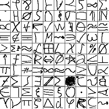
Figure 1: 100 recordings of the HASYv2 data set.

HWRT contains exactly the same recordings and classes as HASY, but HASY is rendered in order to make it easy to use.

HWRT and hence HASY is a merged dataset. $91.93\text{\,}\mathrm{\char 37\relax}$ of HWRT were collected by Detexify [Kir10, Kir14]. The remaining recordings were collected by http://write-math.com. Both projects aim at helping users to find LaTeX commands in cases where the users know how to write the symbol, but not the symbols name. The user writes the symbol on a blank canvas in the browser (either via touch devices or with a mouse). Then the websites give the Top-$k$ results which the user could have thought of. The user then clicks on the correct symbol to accept it as the correct symbol. On write-math.com, other users can also suggest which symbol could be the correct one.

After collecting the data, Martin Thoma manually inspected each recording. This manual inspection is a necessary step as anonymous web users could submit any drawing they wanted to any symbol. This includes many creative recordings as shown in [Kir10, Tho14] as well as loose associations. In some cases, the correct label was unambiguous and could be changed. In other cases, the recordings were removed from the data set.

It is not possible to determine the exact number of people who contributed handwritten symbols to the Detexify part of the dataset. The part which was created with write-math.com was created by 477 user IDs. Although user IDs are given in the dataset, they are not reliable. On the one hand, the Detexify data has the user ID 16925, although many users contributed to it. Also, some users lend their phone to others while being logged in to show how write-math.com works. This leads to multiple users per user ID. On the other hand, some users don’t register and use write-math.com multiple times. This can lead to multiple user IDs for one person.

IV Classes

The HASYv2 dataset contains 369 classes. Those classes include the Latin uppercase and lowercase characters (A-Z, a-z), the Arabic numerals (0-9), 32 different types of arrows, fractal and calligraphic Latin characters, brackets and more. See LABEL:table:symbols-of-db-0, VII, VIII, IX, X, XI, XII, XIII and XIV for more information.

V Data

The HASYv2 dataset contains $168\,233$ black and white images of the size $$32\text{\,}\mathrm{px}$\times$32\text{\,}\mathrm{px}$$. Each image is labeled with one of 369 labels. An example of 100 elements of the HASYv2 data set is shown in Figure 1.

The average amount of black pixels is $16\text{\,}\mathrm{\char 37\relax}$, but this is highly class-dependent ranging from $3.7\text{\,}\mathrm{\char 37\relax}$ of “$\dotsc$” to $59.2\text{\,}\mathrm{\char 37\relax}$ of “$\blacksquare$” average black pixel by class.

The ten classes with most recordings are:

$$\int,\sum,\infty,\alpha,\xi,\equiv,\partial,\mathds{R},\in,\square$$

Those symbols have $26\,780$ recordings and thus account for $16\text{\,}\mathrm{\char 37\relax}$ of the data set. 47 classes have more than $1000$ recordings. The number of recordings of the remaining classes are distributed as visualized in Figure 2.

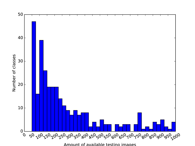
Figure 2: Distribution of the data among classes. 47 classes with more than $1000$ recordings are not shown.

A weakness of HASYv2 is the amount of available data per class. For some classes, there are only 51 elements in the test set.

The data has $32\cdot 32=1024$ features in $\Set{0,255}$. As Table I shows, $32\text{\,}\mathrm{\char 37\relax}$ of the features can explain $90\text{\,}\mathrm{\char 37\relax}$ of the variance, $54\text{\,}\mathrm{\char 37\relax}$ of the features explain $99\text{\,}\mathrm{\char 37\relax}$ of the variance and $86\text{\,}\mathrm{\char 37\relax}$ of the features explain $99\text{\,}\mathrm{\char 37\relax}$ of the variance.

Principal Components	331	551	882
Explained Variance	$90\text{\,}\mathrm{\char 37\relax}$	$95\text{\,}\mathrm{\char 37\relax}$	$99\text{\,}\mathrm{\char 37\relax}$

Table I: The number of principal components necessary to explain, $90\text{\,}\mathrm{\char 37\relax}$, $95\text{\,}\mathrm{\char 37\relax}$, $99\text{\,}\mathrm{\char 37\relax}$ of the data.

The Pearson correlation coefficient was calculated for all features. The features are more correlated the closer the pixels are together as one can see in Figure 3. The block-like structure of every 32th feature comes from the fact the features were flattened for this visualization. The second diagonal to the right shows features which are one pixel down in the image. Those correlations are expected as symbols are written by continuous lines. Less easy to explain are the correlations between high-index features with low-index features in the upper right corner of the image. Those correlations correspond to features in the upper left corner with features in the lower right corner. One explanation is that symbols which have a line in the upper left corner are likely $\blacksquare$.

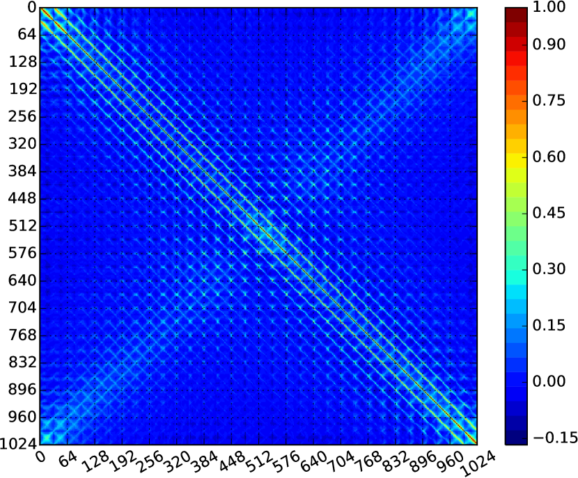
Figure 3: Correlation of all $32\cdot 32=1024$ features. The diagonal shows the correlation of a feature with itself.

VI Classification Challenge

VI-A Evaluation

HASY defines 10 folds which should be used for calculating the accuracy of any classifier being evaluated on HASY as follows:

function CrossValidation(Folds $F$)

     $D\leftarrow\cup_{i=1}^{10}F_{i}$$\triangleright$ Complete Dataset

     for ($i=0$; $\;i<10$; $\;i$++) do

         $A\leftarrow D\setminus F_{i}$$\triangleright$ Train set

         $B\leftarrow F_{i}$$\triangleright$ Test set

         Train Classifier $C_{i}$ on $A$

         Calculate accuracy $a_{i}$ of $C_{i}$ on $B$

     end for

     return ($\frac{1}{10}\sum_{i=1}^{10}a_{i}$, $\min(a_{i})$, $\max(a_{i})$)

end function

Algorithm 1 Calculate the mean accuracy, the minimum accuracy, and the maximum accuracy with 10-fold cross-validation

VI-B Model Baselines

Eight standard algorithms were evaluated by their accuracy on the raw image data. The neural networks were implemented with Tensorflow [AAB⁺15]. All other algorithms are implemented in sklearn [PVG⁺11]. Table II shows the results of the models being trained and tested on MNIST and also for HASYv2:

Classifier	Test Accuracy
	MNIST	HASY	min – max00
TF-CNN	$99.20\text{\,}\mathrm{\char 37\relax}$	$81.0\text{\,}\mathrm{\char 37\relax}$	$80.6\text{\,}\mathrm{\char 37\relax}$ – $81.5\text{\,}\mathrm{\char 37\relax}$
Random Forest	$96.41\text{\,}\mathrm{\char 37\relax}$	$62.4\text{\,}\mathrm{\char 37\relax}$	$62.1\text{\,}\mathrm{\char 37\relax}$ – $62.8\text{\,}\mathrm{\char 37\relax}$
MLP (1 Layer)	$89.09\text{\,}\mathrm{\char 37\relax}$	$62.2\text{\,}\mathrm{\char 37\relax}$	$61.7\text{\,}\mathrm{\char 37\relax}$ – $62.9\text{\,}\mathrm{\char 37\relax}$
LDA	$86.42\text{\,}\mathrm{\char 37\relax}$	$46.8\text{\,}\mathrm{\char 37\relax}$	$46.3\text{\,}\mathrm{\char 37\relax}$ – $47.7\text{\,}\mathrm{\char 37\relax}$
QDA	$55.61\text{\,}\mathrm{\char 37\relax}$	$25.4\text{\,}\mathrm{\char 37\relax}$	$24.9\text{\,}\mathrm{\char 37\relax}$ – $26.2\text{\,}\mathrm{\char 37\relax}$
Decision Tree	$65.40\text{\,}\mathrm{\char 37\relax}$	$11.0\text{\,}\mathrm{\char 37\relax}$	$10.4\text{\,}\mathrm{\char 37\relax}$ – $11.6\text{\,}\mathrm{\char 37\relax}$
Naive Bayes	$56.15\text{\,}\mathrm{\char 37\relax}$	$8.3\text{\,}\mathrm{\char 37\relax}$	$7.9\text{\,}\mathrm{\char 37\relax}$ – 0$8.7\text{\,}\mathrm{\char 37\relax}$
AdaBoost	$73.67\text{\,}\mathrm{\char 37\relax}$	$3.3\text{\,}\mathrm{\char 37\relax}$	$2.1\text{\,}\mathrm{\char 37\relax}$ – 0$3.9\text{\,}\mathrm{\char 37\relax}$

Table II: Classification results for eight classifiers. The number of test samples differs between the folds, but is $$16\,827$\pm 166$. The decision tree was trained with a maximum depth of 5. The exact structure of the CNNs is explained in Section VI-C.

The following observations are noteworthy:

• All algorithms achieve much higher accuracy on MNIST than on HASYv2.

• While a single Decision Tree performs much better on MNIST than QDA, it is exactly the other way around for HASY. One possible explanation is that MNIST has grayscale images while HASY has black and white images.

VI-C Convolutional Neural Networks

Convolutional Neural Networks (CNNs) are state of the art on several computer vision benchmarks like MNIST [WZZ⁺13], CIFAR-10, CIFAR-100 and SVHN [HLW16], ImageNet 2012 [HZRS15] and more. Experiments on HASYv2 without preprocessing also showed that even the simplest CNNs achieve much higher accuracy on HASYv2 than all other classifiers (see Table II).

Table III shows the 10-fold cross-validation results for four architectures.

Network	Parameters	Test Accuracy		Time
		mean	min – max00
2-layer	$3\,023\,537$	$73.8\text{\,}\mathrm{\char 37\relax}$	$72.9\text{\,}\mathrm{\char 37\relax}$ – $74.3\text{\,}\mathrm{\char 37\relax}$	$1.5\text{\,}\mathrm{s}$
3-layer	$1\,530\,609$	$78.4\text{\,}\mathrm{\char 37\relax}$	$77.6\text{\,}\mathrm{\char 37\relax}$ – $79.0\text{\,}\mathrm{\char 37\relax}$	$2.4\text{\,}\mathrm{s}$
4-layer	$848\,753$	$80.5\text{\,}\mathrm{\char 37\relax}$	$79.2\text{\,}\mathrm{\char 37\relax}$ – $80.7\text{\,}\mathrm{\char 37\relax}$	$2.8\text{\,}\mathrm{s}$
TF-CNN	$4\,592\,369$	$81.0\text{\,}\mathrm{\char 37\relax}$	$80.6\text{\,}\mathrm{\char 37\relax}$ – $81.5\text{\,}\mathrm{\char 37\relax}$	$2.9\text{\,}\mathrm{s}$

Table III: Classification results for CNN architectures. The test time is, as before, the mean test time for all examples on the ten folds.

The following architectures were evaluated:

• 2-layer: A convolutional layer with 32 filters of size $3\times 3\times 1$ is followed by a $2\times 2$ max pooling layer with stride 2. The output layer is — as in all explored CNN architectures — a fully connected softmax layer with 369 neurons.

• 3-layer: Like the 2-layer CNN, but before the output layer is another convolutional layer with 64 filters of size $3\times 3\times 32$ followed by a $2\times 2$ max pooling layer with stride 2.

• 4-layer: Like the 3-layer CNN, but before the output layer is another convolutional layer with 128 filters of size $3\times 3\times 64$ followed by a $2\times 2$ max pooling layer with stride 2.

• TF-CNN: A convolutional layer with 32 filters of size $3\times 3\times 1$ is followed by a $2\times 2$ max pooling layer with stride 2. Another convolutional layer with 64 filters of size $3\times 3\times 32$ and a $2\times 2$ max pooling layer with stride 2 follow. A fully connected layer with 1024 units and tanh activation function, a dropout layer with dropout probability 0.5 and the output softmax layer are last. This network is described in [tf-16b].

For all architectures, ADAM [KB14] was used for training. The combined training and testing time was always less than 6 hours for the 10 fold cross-validation on a Nvidia GeForce GTX Titan Black with CUDA 8 and CuDNN 5.1.

VI-D Class Difficulties

The class-wise accuracy

$$\text{class-accuracy}(c)=\frac{\text{correctly predicted samples of class }c}{\text{total number of training samples of class }c}$$

is used to estimate how difficult a class is.

32 classes were not a single time classified correctly by TF-CNN and hence have a class-accuracy of 0. They are shown in Table IV. Some, like \mathsection and \S are not distinguishable at all. Others, like \Longrightarrow and \Rightarrow are only distinguishable in some peoples handwriting. Those classes account for $2.8\text{\,}\mathrm{\char 37\relax}$ of the data.

LaTeX	Rendered	Total	Confused with
\mid	$\mid$	34	|	$|$
\triangle	$\triangle$	32	\Delta	$\Delta$
\mathds{1}	$\mathds{1}$	32	\mathbb{1}	$\mathbb{1}$
\checked	Φ	28	\checkmark	$\checkmark$
\shortrightarrow	$\shortrightarrow$	28	\rightarrow	$\rightarrow$
\Longrightarrow	$\Longrightarrow$	27	\Rightarrow	$\Rightarrow$
\backslash	$\backslash$	26	\setminus	$\setminus$
\O	Ø	24	\emptyset	$\emptyset$
\with	$\with$	21	\&	$\&$
\diameter	Ø	20	\emptyset	$\emptyset$
\triangledown	$\triangledown$	20	\nabla	$\nabla$
\longmapsto	$\longmapsto$	19	\mapsto	$\mapsto$
\dotsc	$\dotsc$	15	\dots	$\dots$
\fullmoon	#	15	\circ	$\circ$
\varpropto	$\varpropto$	14	\propto	$\propto$
\mathsection	$\mathsection$	13	\S	$\S$
\vartriangle	$\vartriangle$	12	\Delta	$\Delta$
O	$O$	9	\circ	$\circ$
o	$o$	7	\circ	$\circ$
c	$c$	7	\subset	$\subset$
v	$v$	7	\vee	$\vee$
x	$x$	7	\times	$\times$
\mathbb{Z}	$\mathbb{Z}$	7	\mathds{Z}	$\mathds{Z}$
T	$T$	6	\top	$\top$
V	$V$	6	\vee	$\vee$
g	$g$	6	9	$9$
l	$l$	6	|	$|$
s	$s$	6	\mathcal{S}	$\mathcal{S}$
z	$z$	6	\mathcal{Z}	$\mathcal{Z}$
\mathbb{R}	$\mathbb{R}$	6	\mathds{R}	$\mathds{R}$
\mathbb{Q}	$\mathbb{Q}$	6	\mathds{Q}	$\mathds{Q}$
\mathbb{N}	$\mathbb{N}$	6	\mathds{N}	$\mathds{N}$

Table IV: 32 classes which were not a single time classified correctly by the best CNN.

In contrast, 21 classes have an accuracy of more than $99\text{\,}\mathrm{\char 37\relax}$ with TF-CNN (see Table V).

LaTeX	Rendered	Total
\forall	$\forall$	214
\sim	$\sim$	201
\nabla	$\nabla$	122
\cup	$\cup$	93
\neg	$\neg$	85
\setminus	$\setminus$	52
\supset	$\supset$	42
\vdots	$\vdots$	41
\boxtimes	$\boxtimes$	22
\nearrow	$\nearrow$	21
\uplus	$\uplus$	19
\nvDash	$\nvDash$	15
\AE	Æ	15
\Vdash	$\Vdash$	14
\Leftarrow	$\Leftarrow$	14
\upharpoonright	$\upharpoonright$	14
-	$-$	12
\guillemotleft	$\guillemotleft$	11
R	$R$	9
7	$7$	8
\blacktriangleright	$\blacktriangleright$	6

Table V: 21 classes with a class-wise accuracy of more than $99\text{\,}\mathrm{\char 37\relax}$ with TF-CNN.

VII Verification Challenge

In the setting of an online symbol recognizer like write-math.com it is important to recognize when the user enters a symbol which is not known to the classifier. One way to achieve this is by training a binary classifier to recognize when two recordings belong to the same symbol. This kind of task is similar to face verification. Face verification is the task where two images with faces are given and it has to be decided if they belong to the same person.

For the verification challenge, a training-test split is given. The training data contains images with their class labels. The test set contains 32 symbols which were not seen by the classifier before. The elements of the test set are pairs of recorded handwritten symbols $(r_{1},r_{2})$. There are three groups of tests:

1. $r_{1}$ and $r_{2}$ both belong to symbols which are in the training set,

2. $r_{1}$ belongs to a symbol in the training set, but $r_{2}$ might not

3. $r_{1}$ and $r_{2}$ don’t belong symbols in the training set

When evaluating models, the models may not take advantage of the fact that it is known if a recording $r_{1}$ / $r_{2}$ is an instance of the training symbols. For all test sets, the following numbers should be reported: True Positive (TP), True Negative (TN), False Positive (FP), False Negative (FN), Accuracy $=\frac{TP+TN}{TP+TN+FP+FN}$.

VIII Acknowledgment

I want to thank “Begabtenstiftung Informatik Karlsruhe”, the Foundation for Gifted Informatics Students in Karlsruhe. Their support helped me to write this work.

Obtaining the data

The data can be found at https://doi.org/10.5281/zenodo.259444. It is a tar.gz file of $34.6\text{\,}\mathrm{MB}$. The file can be verified with the MD5sum

fddf23f36e24b5236f6b3a0880c778e3

The data is published under the ODbL license. If you use the HASY dataset, please cite this paper.

The tar.gz archive contains all data as png images and CSV files with labels. The CSV files have the columns path,symbol_id,latex,user_id with a header row. The path is the relative path to a training example to the CSV file, e.g. ../hasy-data/v2-00000.png. The symbol_id is an internal numeric identifier for the symbol class. The website write-math.com/symbol/?id=[symbol_id] gives information related to the symbol. The column latex contains the LaTeX command associated with the class.

Symbol Classes

LaTeX	Rendered	LaTeX	Rendered
\&	$\&$	\nmid	$\nmid$
\Im	$\Im$	\nvDash	$\nvDash$
\Re	$\Re$	\int	$\int$
\S	$\S$	\fint	$\fint$
\Vdash	$\Vdash$	\odot	$\odot$
\aleph	$\aleph$	\oiint	$\oiint$
\amalg	$\amalg$	\oint	$\oint$
\angle	$\angle$	\varoiint	$\varoiint$
\ast	$\ast$	\ominus	$\ominus$
\asymp	$\asymp$	\oplus	$\oplus$
\backslash	$\backslash$	\otimes	$\otimes$
\between	$\between$	\parallel	$\parallel$
\blacksquare	$\blacksquare$	\parr	$\parr$
\blacktriangleright	$\blacktriangleright$	\partial	$\partial$
\bot	$\bot$	\perp	$\perp$
\bowtie	$\bowtie$	\pitchfork	$\pitchfork$
\boxdot	$\boxdot$	\pm	$\pm$
\boxplus	$\boxplus$	\prime	$\prime$
\boxtimes	$\boxtimes$	\prod	$\prod$
\bullet	$\bullet$	\propto	$\propto$
\checkmark	$\checkmark$	\rangle	$\rangle$
\circ	$\circ$	\rceil	$\rceil$
\circledR	$\circledR$	\rfloor	$\rfloor$
\circledast	$\circledast$	\rrbracket	$\rrbracket$
\circledcirc	$\circledcirc$	\rtimes	$\rtimes$
\clubsuit	$\clubsuit$	\sharp	$\sharp$
\coprod	$\coprod$	\sphericalangle	$\sphericalangle$
\copyright	$\copyright$	\sqcap	$\sqcap$
\dag	${\dagger}$	\sqcup	$\sqcup$
\dashv	$\dashv$	\sqrt{}	$\sqrt{}$
\diamond	$\diamond$	\square	$\square$
\diamondsuit	$\diamondsuit$	\star	$\star$
\div	$\div$	\sum	$\sum$
\ell	$\ell$	\times	$\times$
\flat	$\flat$	\top	$\top$
\frown	$\frown$	\triangle	$\triangle$
\guillemotleft	$\guillemotleft$	\triangledown	$\triangledown$
\hbar	$\hbar$	\triangleleft	$\triangleleft$
\heartsuit	$\heartsuit$	\trianglelefteq	$\trianglelefteq$
\infty	$\infty$	\triangleq	$\triangleq$
\langle	$\langle$	\triangleright	$\triangleright$
\lceil	$\lceil$	\uplus	$\uplus$
\lfloor	$\lfloor$	\vDash	$\vDash$
\lhd	$\lhd$	\varnothing	$\varnothing$
\lightning	$\lightning$	\varpropto	$\varpropto$
\llbracket	$\llbracket$	\vartriangle	$\vartriangle$
\lozenge	$\lozenge$	\vdash	$\vdash$
\ltimes	$\ltimes$	\with	$\with$
\mathds{1}	$\mathds{1}$	\wp	$\wp$
\mathsection	$\mathsection$	\wr	$\wr$
\mid	$\mid$	\{	$\{$
\models	$\models$	\|	$\|$
\mp	$\mp$	\}	$\}$
\multimap	$\multimap$	\vee	$\vee$
\nabla	$\nabla$	\wedge	$\wedge$
\neg	$\neg$	\barwedge	$\barwedge$

Table VI: 112 symbols of HASY.

LaTeX	Rendered	LaTeX	Rendered	LaTeX	Rendered	LaTeX	Rendered
\#	$\#$	A	$A$	S	$S$	i	$i$
\$	$\$$	B	$B$	T	$T$	j	$j$
\%	$\%$	C	$C$	U	$U$	k	$k$
+	$+$	D	$D$	V	$V$	l	$l$
-	$-$	E	$E$	W	$W$	m	$m$
/	$/$	F	$F$	X	$X$	n	$n$
0	$0$	G	$G$	Y	$Y$	o	$o$
1	$1$	H	$H$	Z	$Z$	p	$p$
2	$2$	I	$I$	[	$[$	q	$q$
3	$3$	J	$J$	]	$]$	r	$r$
4	$4$	K	$K$	a	$a$	s	$s$
5	$5$	L	$L$	b	$b$	u	$u$
6	$6$	M	$M$	c	$c$	v	$v$
7	$7$	N	$N$	d	$d$	w	$w$
8	$8$	O	$O$	e	$e$	x	$x$
9	$9$	P	$P$	f	$f$	y	$y$
<	$<$	Q	$Q$	g	$g$	z	$z$
>	$>$	R	$R$	h	$h$	|	$|$

Table VII: 72 ASCII symbols of HASY, including all ten digits, the Latin alphabet in lower and upper case and a few more symbols.

LaTeX	Rendered	LaTeX	Rendered	LaTeX	Rendered
\approx	$\approx$	\geqslant	$\geqslant$	\lesssim	$\lesssim$
\doteq	$\doteq$	\neq	$\neq$	\backsim	$\backsim$
\simeq	$\simeq$	\not\equiv	$\not\equiv$	\sim	$\sim$
\equiv	$\equiv$	\preccurlyeq	$\preccurlyeq$	\succ	$\succ$
\geq	$\geq$	\preceq	$\preceq$	\prec	$\prec$
\leq	$\leq$	\succeq	$\succeq$	\gtrless	$\gtrless$
\leqslant	$\leqslant$	\gtrsim	$\gtrsim$	\cong	$\cong$

Table VIII: 21 symbols which are in HASYand indicate a relationship.

LaTeX	Rendered	LaTeX	Rendered
\Downarrow	$\Downarrow$	\nrightarrow	$\nrightarrow$
\Leftarrow	$\Leftarrow$	\rightarrow	$\rightarrow$
\Leftrightarrow	$\Leftrightarrow$	\rightleftarrows	$\rightleftarrows$
\Longleftrightarrow	$\Longleftrightarrow$	\rightrightarrows	$\rightrightarrows$
\Longrightarrow	$\Longrightarrow$	\rightsquigarrow	$\rightsquigarrow$
\Rightarrow	$\Rightarrow$	\searrow	$\searrow$
\circlearrowleft	$\circlearrowleft$	\shortrightarrow	$\shortrightarrow$
\circlearrowright	$\circlearrowright$	\twoheadrightarrow	$\twoheadrightarrow$
\curvearrowright	$\curvearrowright$	\uparrow	$\uparrow$
\downarrow	$\downarrow$	\rightharpoonup	$\rightharpoonup$
\hookrightarrow	$\hookrightarrow$	\rightleftharpoons	$\rightleftharpoons$
\leftarrow	$\leftarrow$	\longmapsto	$\longmapsto$
\leftrightarrow	$\leftrightarrow$	\mapsfrom	$\mapsfrom$
\longrightarrow	$\longrightarrow$	\mapsto	$\mapsto$
\nRightarrow	$\nRightarrow$	\leadsto	$\leadsto$
\nearrow	$\nearrow$	\upharpoonright	$\upharpoonright$

Table IX: 32 arrow symbols of HASY.

LaTeX	Rendered	LaTeX	Rendered	LaTeX	Rendered
\alpha	$\alpha$	\xi	$\xi$	\Xi	$\Xi$
\beta	$\beta$	\pi	$\pi$	\Pi	$\Pi$
\gamma	$\gamma$	\rho	$\rho$	\Sigma	$\Sigma$
\delta	$\delta$	\sigma	$\sigma$	\Phi	$\Phi$
\epsilon	$\epsilon$	\tau	$\tau$	\Psi	$\Psi$
\zeta	$\zeta$	\phi	$\phi$	\Omega	$\Omega$
\eta	$\eta$	\chi	$\chi$	\varepsilon	$\varepsilon$
\theta	$\theta$	\psi	$\psi$	\varkappa	$\varkappa$
\iota	$\iota$	\omega	$\omega$	\varpi	$\varpi$
\kappa	$\kappa$	\Gamma	$\Gamma$	\varrho	$\varrho$
\lambda	$\lambda$	\Delta	$\Delta$	\varphi	$\varphi$
\mu	$\mu$	\Theta	$\Theta$	\vartheta	$\vartheta$
\nu	$\nu$	\Lambda	$\Lambda$

Table X: All Greek letters and some variations of Greek letters were used for evaluation. 38 of them are in this table, the rest is identical to Latin letters.

LaTeX	Rendered	LaTeX	Rendered	LaTeX	Rendered
\mathcal{A}	$\mathcal{A}$	\mathcal{T}	$\mathcal{T}$	\mathds{Z}	$\mathds{Z}$
\mathcal{B}	$\mathcal{B}$	\mathcal{U}	$\mathcal{U}$	\mathfrak{A}	$\mathfrak{A}$
\mathcal{C}	$\mathcal{C}$	\mathcal{X}	$\mathcal{X}$	\mathfrak{M}	$\mathfrak{M}$
\mathcal{D}	$\mathcal{D}$	\mathcal{Z}	$\mathcal{Z}$	\mathfrak{S}	$\mathfrak{S}$
\mathcal{E}	$\mathcal{E}$	\mathbb{H}	$\mathbb{H}$	\mathfrak{X}	$\mathfrak{X}$
\mathcal{F}	$\mathcal{F}$	\mathbb{N}	$\mathbb{N}$	\mathscr{A}	$\mathscr{A}$
\mathcal{G}	$\mathcal{G}$	\mathbb{Q}	$\mathbb{Q}$	\mathscr{C}	$\mathscr{C}$
\mathcal{H}	$\mathcal{H}$	\mathbb{R}	$\mathbb{R}$	\mathscr{D}	$\mathscr{D}$
\mathcal{L}	$\mathcal{L}$	\mathbb{Z}	$\mathbb{Z}$	\mathscr{E}	$\mathscr{E}$
\mathcal{M}	$\mathcal{M}$	\mathds{C}	$\mathds{C}$	\mathscr{F}	$\mathscr{F}$
\mathcal{N}	$\mathcal{N}$	\mathds{E}	$\mathds{E}$	\mathscr{H}	$\mathscr{H}$
\mathcal{O}	$\mathcal{O}$	\mathds{N}	$\mathds{N}$	\mathscr{L}	$\mathscr{L}$
\mathcal{P}	$\mathcal{P}$	\mathds{P}	$\mathds{P}$	\mathscr{P}	$\mathscr{P}$
\mathcal{R}	$\mathcal{R}$	\mathds{Q}	$\mathds{Q}$	\mathscr{S}	$\mathscr{S}$
\mathcal{S}	$\mathcal{S}$	\mathds{R}	$\mathds{R}$

Table XI: 44 variants of Latin letters in HASY.

LaTeX	Rendered	LaTeX	Rendered	LaTeX	Rendered
\therefore	$\therefore$	\cdot	$\cdot$	\dots	$\dots$
\because	$\because$	\vdots	$\vdots$	\ddots	$\ddots$
\dotsc	$\dotsc$

Table XII: 7 symbols that contain only dots in HASY.

LaTeX	R	LaTeX	R	LaTeX	R	LaTeX	R	LaTeX	R
\AA	Å	\L		\male	æ	\ohm	$\Omega$	\sun	.
\AE		\O		\mars	æ	\fullmoon	#	\degree	∘
\aa	å	\o		\female	ß	\leftmoon	$	\iddots
\ae		\Bowtie	1	\venus	ß	\checked	Φ	\diameter	Ø
\ss		\celsius	${}^{\circ}\mathrm{C}$	\astrosun	$\odot$	\pounds	£	\mathbb{1}

Table XIII: 25 symbols of HASY.

LaTeX	Rendered	LaTeX	Rendered	LaTeX	Rendered
\cup	$\cup$	\varsubsetneq	$\varsubsetneq$	\exists	$\exists$
\cap	$\cap$	\nsubseteq	$\nsubseteq$	\nexists	$\nexists$
\emptyset	$\emptyset$	\sqsubseteq	$\sqsubseteq$	\forall	$\forall$
\setminus	$\setminus$	\subseteq	$\subseteq$	\in	$\in$
\supset	$\supset$	\subsetneq	$\subsetneq$	\ni	$\ni$
\subset	$\subset$	\supseteq	$\supseteq$	\notin	$\notin$

Table XIV: 18 set related symbols of HASY.

References

- [AAB+15] M. Abadi, A. Agarwal, P. Barham, E. Brevdo, Z. Chen, C. Citro, G. S. Corrado, A. Davis, J. Dean, M. Devin, S. Ghemawat, I. Goodfellow, A. Harp, G. Irving, M. Isard, Y. Jia, R. Jozefowicz, L. Kaiser, M. Kudlur, J. Levenberg, D. Mané, R. Monga, S. Moore, D. Murray, C. Olah, M. Schuster, J. Shlens, B. Steiner, I. Sutskever, K. Talwar, P. Tucker, V. Vanhoucke, V. Vasudevan, F. Viégas, O. Vinyals, P. Warden, M. Wattenberg, M. Wicke, Y. Yu, and X. Zheng, “TensorFlow: Large-scale machine learning on heterogeneous systems,” 2015, software available from tensorflow.org. [Online]. Available: http://tensorflow.org/
- [HLW16] G. Huang, Z. Liu, and K. Q. Weinberger, “Densely connected convolutional networks,” arXiv preprint arXiv:1608.06993, Aug. 2016. [Online]. Available: https://arxiv.org/abs/1608.06993v1
- [HZRS15] K. He, X. Zhang, S. Ren, and J. Sun, “Deep residual learning for image recognition,” arXiv preprint arXiv:1512.03385, Dec. 2015. [Online]. Available: https://arxiv.org/pdf/1512.03385v1.pdf
- [KB14] D. Kingma and J. Ba, “Adam: A method for stochastic optimization,” arXiv preprint arXiv:1412.6980, Dec. 2014. [Online]. Available: https://arxiv.org/abs/1412.6980
- [Kir10] D. Kirsch, “Detexify: Erkennung handgemalter LaTeX-symbole,” Diploma thesis, Westfälische Wilhelms-Universität Münster, 10 2010. [Online]. Available: http://danielkirs.ch/thesis.pdf
- [Kir14] ——, “Detexify data,” Jul. 2014. [Online]. Available: https://github.com/kirel/detexify-data
- [LBBH98] Y. LeCun, L. Bottou, Y. Bengio, and P. Haffner, “Gradient-based learning applied to document recognition,” Proceedings of the IEEE, vol. 86, no. 11, pp. 2278–2324, Nov. 1998. [Online]. Available: http://yann.lecun.com/exdb/publis/pdf/lecun-01a.pdf
- [PVG+11] F. Pedregosa, G. Varoquaux, A. Gramfort, V. Michel, B. Thirion, O. Grisel, M. Blondel, P. Prettenhofer, R. Weiss, V. Dubourg, J. Vanderplas, A. Passos, D. Cournapeau, M. Brucher, M. Perrot, and E. Duchesnay, “Scikit-learn: Machine learning in Python,” Journal of Machine Learning Research, vol. 12, pp. 2825–2830, 2011.
- [TF-16a] “Deep mnist for experts,” Dec. 2016. [Online]. Available: https://www.tensorflow.org/tutorials/mnist/pros/
- [tf-16b] “Deep mnist for experts,” Dec. 2016. [Online]. Available: https://www.tensorflow.org/tutorials/mnist/pros/
- [Tho14] M. Thoma, “On-line Recognition of Handwritten Mathematical Symbols,” Bachelor’s Thesis, Karlsruhe Institute of Technology, Karlsruhe, Germany, Nov. 2014. [Online]. Available: http://martin-thoma.com/write-math
- [WZZ+13] L. Wan, M. Zeiler, S. Zhang, Y. L. Cun, and R. Fergus, “Regularization of neural networks using dropconnect,” in Proceedings of the 30th International Conference on Machine Learning (ICML-13), 2013, pp. 1058–1066. [Online]. Available: http://www.matthewzeiler.com/pubs/icml2013/icml2013.pdf