On connections of the Liénard equation with some equations of Painlevé–Gambier type

Abstract

The Liénard equation is used in various applications. Therefore, constructing general analytical solutions of this equation is an important problem. Here we study connections between the Liénard equation and some equations from the Painlevé–Gambier classification. We show that with the help of such connections one can construct general analytical solutions of the Liénard equation’s subfamilies. In particular, we find three new integrable families of the Liénard equation. We also propose and discuss an approach for finding one–parameter families of closed–form analytical solutions of the Liénard equation.

Keywords: Liénard equation; analytical solution; Sundman transformation; Painlevé-Gambier classification.

1 Introduction

We consider the Liénard equation

$$y_{zz}+f(y)y_{z}+g(y)=0,$$ (1)

where $f$ and $g$ are arbitrary functions, which do not vanish simultaneously. Equation (1) has a vast range of applications in physics, biology and other fields of science [1, 2, 3, 4].

The Liénard equation has been thoroughly investigated from a dynamical systems point of view (see, e.g. [5, 6, 7, 8] and references therein). However, only a few studies were devoted to the construction of closed–form analytical solutions of the Liénard equation. For instance, Lie point symmetries of equation (1) were studied in [9, 10, 11] and equations having eight, three and two parameters symmetries, i.e. those equations that can be integrated by the Lie method, were found. Integrability of the Liénard equation with the help of the Prelle–Singer method was considered in [12] and some integrable Liénard equations were constructed. Authors of [13, 14] found necessary and sufficient conditions for linearization of the Liénard–type equation via the generalized Sundman transformations. In [15] it was shown that integrability conditions for equation (1) obtained with the help of the Chiellini lemma (see, e.g. [16, 17]) are equivalent to linearizabiliy conditions via the generalized Sundman transformations. Moreover, authors of [15] also pointed out that equation (1) with a maximal point symmetries group can be linearized by the generalized Sundman transformations.

Recently in [18, 19, 20, 15] it has been shown that new families of integrable Liénard equations can be constructed if one considers connections between the Liénard–type equations and some other nonlinear differential equations, which have the closed–form general analytical solutions. Let us remark that both in [18, 19, 20, 15] and in this work it is supposed that such connections are given by the generalized Sundman transformations. For example, authors of [20] proved that the quadratic Liénard equation (see, e.g. [21, 22]) can be mapped into an equation for the elliptic functions via the generalized Sundman transformations for arbitrary coefficients. In [15] a new criterion for the integrability of equation (1) was proposed using a connection between the Liénard equation and a sub–case of equation (1) which general solution can be expressed via the Jacobi elliptic cosine. Here we extend results of [15] and study connections between equation (1) and its sub–cases that are of the Painlevé–Gambier type (see, e.g. [23]). As a result, we find three new families of integrable Liénard equations. We also propose an approach for constructing one–parameter families of analytical solutions of equation (1). To the best of our knowledge our results are new.

The rest of this work is organized as follows. In the next section we study connections between the Liénard equation and some equations of the Painlevé–Gambier type and obtain three new criteria for integrability of the Liénard equation. We also discuss an approach for constructing one–parameter families of analytical solutions of equation (1). We demonstrate effectiveness of our approaches by several new examples of integrable Liénard equations in section 3. In the last section we briefly discuss our results.

2 Main results

We study connections of the Liénard equation with some equations from the Painlevé–Gambier classification that are given by the nonlocal transformations

$$w=F(y),\quad d\zeta=G(y)dz,\quad F_{y}G\neq 0,$$ (2)

where $w$ and $\zeta$ are new dependent and independent variables correspondingly. Transformations (2) are called the generalized Sundaman transformations (see, e.g. [13, 14]).

Let us note that throughout this work we consider only autonomous equations from the Painlevé–Gambier classification. Thus, when we discuss a certain Painlevé–Gambier type equation with variable coefficients we assume that these coefficients are constants. There are seven subcases of equation (1) with $f(y)\not\equiv 0$ that belong to the Painlevé–Gambier classification [23]. They are non–canonical forms of equations II, V and VII and equations VI, X, XXIV and XVII from Ince’s book [23] (in the last two equations it is assumed that the parameter $m$ is equal to 1).

It can be seen that equations VI, X and XXIV can be linearized by transformations (2) (see [13, 15]). Therefore, equations from (1) which can be transformed into VI, X and XXIV by means of (2) can be linearized via (2) since a combination of Sundman transformations is a Sundman transformation. A connection between (1) and equation VII has been recently studied in [15]. Consequently, it is necessary to study connections between (1) and equations II, V and XVII. These connections lead us to new criteria for integrability of the Liénard equations.

2.1 Equation II from the Painlevé–Gambier classification

First of all, we consider the following non–canonical form of equation II from the Painlevé–Gambier classification [23]

$$w_{\zeta\zeta}+5w_{\zeta}+6w-w^{2}=0.$$ (3)

The general solution of equation (3) can be written as follows

$$w=6e^{-2(\zeta-\zeta_{0})}\wp\left\{e^{-(\zeta-\zeta_{0})},0,g_{3}\right\},$$ (4)

where $\wp$ is the Weierstrass elliptic function and $g_{3}$ is an arbitrary constant. Let us note that throughout this work we denote by $\zeta_{0}$ an arbitrary constant corresponding to the invariance of the studied equations under shift transformations in an independent variable.

There is a non–autonomous first integral of equation (3):

$$6(w_{\zeta}+2w)^{2}-4w^{3}=216g_{3}e^{-6\zeta}.$$ (5)

Below we show that relation (5) can be used for the construction of one–parametric analytical solutions of the Liénard equation. Notice also that solution (4) degenerates in the case of $g_{3}=0$ and can be found from (4):

$$w=6(e^{\zeta-\zeta_{0}}+1)^{-2}.$$ (6)

Now we discuss a connection between the whole family of the Liénard equations and equation (4).

Theorem 1. Equation (1) can be transformed into (3) by means of (2) with

$$F=\kappa\left(\int fdy+\lambda\right),\quad G(y)=\frac{1}{5}f,$$ (7)

if the following correlation on functions $f$ and $g$ holds

$$g=-\frac{f}{25}\left[\int fdy+\lambda\right]\left[\kappa\left(\int fdy+\lambda\right)-6\right],$$ (8)

where $\kappa\neq 0$ and $\lambda$ are arbitrary parameters.
Proof. Using transformations (2) we can express derivatives of $y$ with respect to $z$ via derivatives of $w$ with respect to $\zeta$. Then we substitute these expressions into equation (1) and require that the result is equation (3). As a consequence, we obtain a system of two ordinary differential equations on functions $F$ and $G$ and a correlation on functions $f(y)$ and $g(y)$. Solving these equations with respect to $F$, $G$ and $g$ we get formulas (7) and (8). This completes the proof.

Since equation (1) under condition (8) is connected with (3) via (2) one can suppose that we can obtain a first integral of (1) under (8) form first integral (5) of (3). However, first integral (5) is non–autonomous and we can obtain a first order integro–differential equation for solutions of equation (1) under condition (8). Therefore, we get the following consequence of Theorem 1.

Corollary 1. If condition (8) holds, then solutions of equation (1) satisfy the following relation

$$\begin{gathered}6\kappa^{2}\left[5y_{z}+2\left(\int fdy+\lambda\right)\right]^{2}-4\kappa^{3}\left(\int fdy+\lambda\right)^{3}=216e^{-6\zeta}g_{3},\\ \zeta=\frac{1}{5}\int\limits_{0}^{z}f[y(\xi)]d\xi,\end{gathered}$$ (9)

Note that here and below we denote by $\xi$ a dummy integration variable.

At first glace it may seen that relation (9) is not useful. However, assuming that $g_{3}=0$ in (9) we obtain a first order ordinary differential equation the general solution of which gives us a one–parameter solutions family of equation (1). In the next section we will demonstrate applications of Theorem 1 and Corollary 1 for finding closed–form analytical solutions of the Liénard equation.

2.2 Equation V from the Painlevé–Gambier classification

The next equation that we consider is a non–canonical form of number V equation from the Painlevé–Gambier classification (see [23], p. 331)

$$w_{\zeta\zeta}+2ww_{\zeta}-\alpha(w_{\zeta}+w^{2})+\beta=0,$$ (10)

where $\alpha\neq 0$, $\beta$ are arbitrary parameters.

The general solution of equation (10) has the form

$$w=\frac{\Psi_{\zeta}}{\Psi},\,\,\,\Psi=C_{2}I_{\chi}\left(\frac{2\sqrt{C_{1}}}{\alpha}e^{\alpha\zeta/2}\right)+C_{3}K_{\chi}\left(\frac{2\sqrt{C_{1}}}{\alpha}e^{\alpha\zeta/2}\right),\,\,\,\chi^{2}=\frac{4\beta}{\alpha^{3}},$$ (11)

where $I_{\chi}$, $K_{\chi}$ are the modified Bessel functions, $C_{1}$ and $C_{2}^{2}+C_{3}^{2}\neq 0$ are arbitrary constants. Let us remark that in fact solution (11) depends only on two arbitrary constants and without loss of generality either $C_{2}$ or $C_{3}$ can be set equal to 1.

Equation (10) admits the following non–autonomous first integral

$$w_{\zeta}+w^{2}-\frac{\beta}{\alpha}=C_{1}e^{\alpha\zeta}.$$ (12)

Thus, using (12) we get a special solution of equation (10) corresponding to the case of $C_{1}=0$:

$$w=\sqrt{\frac{\beta}{\alpha}}\tanh\left\{\sqrt{\frac{\beta}{\alpha}}(\zeta-\zeta_{0})\right\}.$$ (13)

Notice that in the case of $\beta=0$ one–parameter family of solutions of (10) has the form $w=(\zeta-\zeta_{0})^{-1}$.

Now we are in position to obtain a criterion of equivalence between equations (1) and (10).

Theorem 2. Suppose that the following correlation on functions $f$ and $g$ holds

$$\begin{gathered}g=\mp\frac{f}{\nu\sqrt{\mu+\nu\int fdy}}\left(\alpha\left[\alpha\pm\sqrt{\mu+\nu\int fdy}\right]^{2}-4\beta\right),\end{gathered}$$ (14)

where $\mu$ and $\nu\neq 0$ are arbitrary parameters; then equation (1) can be transformed into (10) by means of (2) with

$$\begin{gathered}F=\frac{1}{2}\left(\alpha\pm\sqrt{\mu+\nu\int fdy}\right),\quad G=\pm\frac{f}{\sqrt{\mu+\nu\int fdy}}.\end{gathered}$$ (15)

Proof. The proof is similar to that of Theorem 1, and is omitted.

As a straightforward consequence of Theorem 2 we obtain the following result.

Corollary 2. Suppose that correlation (14) holds; then solutions of equation (1) satisfy the following relation

$$\frac{\nu}{4}y_{z}+\left(\frac{\alpha}{2}\pm\frac{1}{2}\sqrt{\mu+\nu\int fdy}\right)^{2}-\frac{\beta}{\alpha}=C_{1}\exp\left\{\pm\alpha\int_{0}^{z}G(y(\xi))d\xi\right\},$$ (16)

where $G$ is given by (15).

One can find special solutions of equation (1) under condition (14) if we assume that $C_{1}=0$ in (16) and solve corresponding first order differential equation. Applications of Theorem 2 and Corollary 2 will be considered in the next section.

2.3 Equation XXVII from the Painlevé–Gambier classification

Now we consider a special case of equation XXVII from the Painlevé–Gambier classification (see [23], p. 338 ). We suppose that $m=1$, $f=\phi=0$ and $\psi=\gamma$, where $\gamma\neq 0$ is an arbitrary parameter. Then equation XXVII takes the form

$$w_{\zeta\zeta}-\frac{1}{w}w_{\zeta}-\gamma w+\frac{1}{w}=0.$$ (17)

Note that connection between equation (1) and the general case of equation XXVII at $m=1$ will be considered elsewhere.

The general solution of equation (17) is given by

$$w=\frac{1}{\sqrt{\gamma}}\cosh\{\sqrt{\gamma}(\zeta-\zeta_{0})\}\bigg{[}\mbox{arctan}\big{(}\sinh\{\sqrt{\gamma}(\zeta-\zeta_{0})\}\big{)}+C_{4}\bigg{]},$$ (18)

where $C_{4}$ is an arbitrary constant.

We can write a first integral of equation (17) as follows

$$\frac{w_{\zeta}-1}{w}=\sqrt{\gamma}\frac{e^{\sqrt{\gamma}\zeta}-C_{5}e^{-\sqrt{\gamma}\zeta}}{e^{\sqrt{\gamma}\zeta}+C_{5}e^{-\sqrt{\gamma}\zeta}},$$ (19)

where $C_{5}$ is an arbitrary constant, which is connected with $\zeta_{0}$.

In the case of $C_{5}=0$ corresponding special solution of equation (17) has the form

$$w=e^{\sqrt{\gamma}(\zeta-\zeta_{0})}-\frac{1}{\sqrt{\gamma}}.$$ (20)

Now we consider a connection between (1) and equation (17).

Theorem 3. Equation (1) can be transformed into (17) by means of (2) with

$$\begin{gathered}F=\sigma\exp\left\{\eta\int fdy\right\},\quad G=-\sigma f\exp\left\{\eta\int fdy\right\},\end{gathered}$$ (21)

if the following correlation on functions $f$ and $g$ holds

$$\begin{gathered}g=-\frac{f}{\eta}\left(\sigma^{2}\gamma\exp\left\{2\eta\int fdy\right\}-1\right),\end{gathered}$$ (22)

where $\sigma\neq 0$ and $\eta\neq 0$ are arbitrary parameters.

Proof. The proof is similar to that of Theorem 1, and is omitted.

Theorem 3 leads us to the following statement.

Corollary 3. If correlation (22) holds, then solutions of equation (1) satisfy the relation

$$\begin{gathered}\exp\left\{-\eta\int fdy\right\}\left(\eta y_{z}+1\right)=-\sigma\sqrt{\gamma}\frac{e^{\sqrt{\gamma}\zeta}-C_{5}e^{-\sqrt{\gamma}\zeta}}{e^{\sqrt{\gamma}\zeta}+C_{5}e^{-\sqrt{\gamma}\zeta}},\\ \zeta=\int\limits_{0}^{z}G(y(\xi))d\xi.\end{gathered}$$ (23)

Here $G$ is given by (21).

In the case of $C_{5}=0$ from (23) we get an ordinary differential equation which general solution gives us a one–parametric family of solutions of equation (1) under correlation (22).

Finally, it is worth noting that criteria for the integrability of equation (1) obtained in Theorems 1–3 do not coincide with previously known integrability conditions for the Liénard equation. Therefore, formulas (8), (14) and (22) give us new families of integrable Liénard equations. Note also that with the help of results form [9, 10, 11] one can see that equation (1) under conditions (8), (14) and (22) cannot be either integrated or linearized by the Lie method.

3 Examples

In this section we consider applications of above obtained connections between the Liénard equation and equations of the Painlevé–Gambier type. We use these results for constructing both general and particular solutions of several members of equations family (1).

3.1 Example of Theorem 1 application.

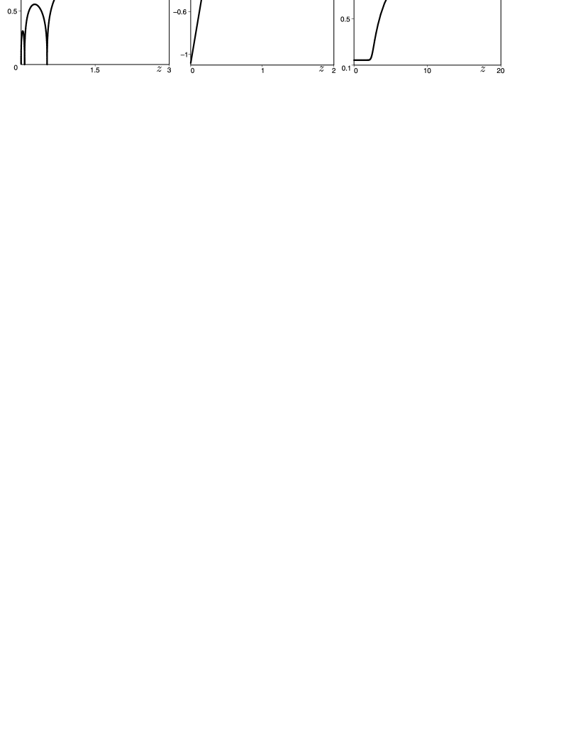
Figure 1: Solution (26) at: a) $a=\lambda=1$, $\kappa=-100$, $g_{3}=1$ and $\zeta_{0}=2.2$; b) $a=\lambda=\kappa=1$, $g_{3}=-1$ and $\zeta_{0}=0.5$; c) $a=\lambda=1$, $\kappa$=-1, $g_{3}=0$ and $\zeta_{0}=25$.

Let us consider the case of $f(y)=a/y^{2}$, where $a\neq 0$ is an arbitrary parameter. With the help of Theorem 1 we find that

$$F(y)=-\frac{a\kappa}{y}+\kappa\lambda,\quad G(y)=\frac{a}{5y^{2}}.$$ (24)

Using (1) and (8) we find corresponding Liénard equation

$$y_{zz}+\frac{a}{y^{2}}y_{z}-\frac{a}{25y^{4}}\left(\lambda y-a\right)\left([\lambda\kappa-6]y-a\kappa\right)=0.$$ (25)

Taking into consideration formulas (2), (4), (24) we get the general solution of equation (25)

$$\begin{gathered}y=\frac{a\kappa}{\lambda\kappa-6e^{-2(\zeta-\zeta_{0})}\wp\left\{e^{-(\zeta-\zeta_{0})},0,g_{3}\right\}},\quad z=\frac{5}{a}\int y^{2}d\zeta.\end{gathered}$$ (26)

In the degenerated case, i.e. when $g_{3}=0$, solution (26) becomes

$$y=\frac{a\kappa(e^{\zeta-\zeta_{0}}+1)^{2}}{\kappa\lambda(e^{\zeta-\zeta_{0}}+1)^{2}-6},\quad z=\frac{5}{a}\int y^{2}d\zeta.$$ (27)

We demonstrate plots of solutions (26), (27) in Fig.1 (plates a,b and plate c correspondingly). We see that these solutions describe various kink–type structures including a kink with oscillatory structure.

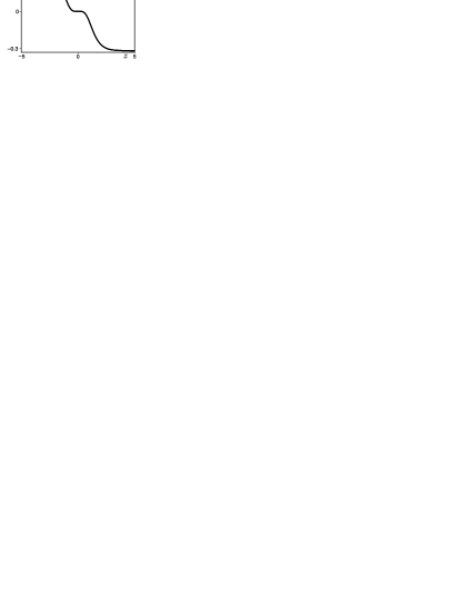
Figure 2: Solution (29) of Eq. (28) at $a=10$ and $z_{0}=0$.

Now we demonstrate an example of Corollary’s 1 application. We assume that $\lambda=0$, $\kappa=3/2$ and $f(y)=4/5ay^{-1/5}$, where $a\neq 0$ is an arbitrary parameter. Then from (1) and (8) we get

$$y_{zz}+\frac{4a}{5}y^{-1/5}y_{z}-\frac{4a^{2}}{125}y^{3/5}\left(\frac{3}{2}ay^{4/5}-6\right)=0.$$ (28)

Using Corollary 1 and solving corresponding first order differential equation we find a one–parameter family of solutions of equation (28)

$$y=-\frac{4\sqrt{2}}{a^{5/4}}\tanh^{5}\left\{\frac{\sqrt{2}a^{5/4}}{25}(z-z_{0})\right\}.$$ (29)

Note that here and below we denote by $z_{0}$ an arbitrary constant. One can see that solution (29) describes a kink–type structure and its plot is demonstrated in Fig.2.

3.2 Example of Theorem 2 application.

Now we give an example of application of Theorem 2. We suppose that $\mu=a^{2}$, $\nu=1$ and $f(y)=4y^{3}+4ay$, where $a$ is an arbitrary parameter. In this case with the help of (14) we find corresponding Liénard equation

$$y_{zz}+(4y^{3}+4ay)y_{z}-4\alpha y(y^{2}+a+\alpha)^{2}+16\beta y=0$$ (30)

The general solution of equation (30) can be obtained with the help of formulas (15) and has the form

$$y=\pm\sqrt{2w-\alpha-a},\quad z=\int\frac{1}{4y}d\zeta,$$ (31)

where $w$ is given by (11). Let us remark that we use the upper sign in formulas (14), (15).

We demonstrate plots of solution (31) corresponding to the plus sing at various values of the parameters in Fig. 3. One can see that solution (31) describes various kink–type structures.

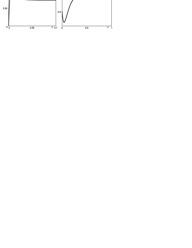
Figure 3: Solution (31) of equation (30) at: a) $\alpha=-1$, $\beta=-10$ and $a=-5$ ; b) $\alpha=-1$, $\beta=-2$ and $a=-3$.

Let us consider an example of Corollary’s 2 application. Suppose that $f=e^{-y}(2\alpha-2e^{-y})$, $\nu=1$ and $\mu=\alpha^{2}$. Then we find a Liénard equation satisfying correlation (14):

$$y_{zz}-2e^{-y}(e^{-y}-\alpha)y_{z}+2e^{-y}(\alpha e^{-2y}-4\beta)=0.$$ (32)

Substituting values of $f$, $\mu$ and $\nu$ into (16) and solving corresponding differential equation we obtain

$$y=\frac{1}{2\alpha}\left[8\beta(z-z_{0})+\alpha\ln\left\{\frac{1}{4\beta}(\alpha e^{-\frac{8\beta}{\alpha}(z-z_{0})}-1)\right\}\right].$$ (33)

Thus, we find a one–parameter family of analytical solutions of equation (32).

3.3 Example of Theorem 3 application.

Now we study applications of Theorem 3. We suppose that $f(y)=(2y+a)/(y^{2}+ay+b)$ and $\eta=1$. Then, using formula (22) we find the following Liénard equation

$$y_{zz}+\frac{2y+a}{y^{2}+ay+b}y_{z}-\frac{2y+a}{y^{2}+ay+b}\left(\sigma^{2}\gamma(y^{2}+ay+b)^{2}-1\right)=0.$$ (34)

The general solution of equation (34) can be obtained with the help of formulas (18) and (21):

$$y=\frac{1}{2}\left(-a\pm\sqrt{\frac{4w}{\sigma}+a^{2}-4b}\right),\quad z=-\int\frac{1}{\sigma(2y+1)}d\zeta,$$ (35)

where $w$ is given by (18). Let us remark that solution (18), and therefore (35) can have a real period in the case of $\gamma<0$. We demonstrate solution (35) corresponding to the plus sing in (35) in Fig.4.

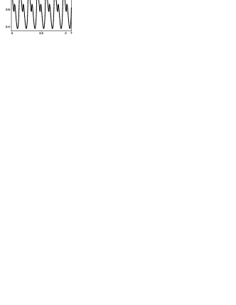
Figure 4: Solution (35) at $\gamma=-\sigma=-2$, $C_{4}=i$, $\zeta_{0}=1/2$, $a=-b=1$.

Corollary 3 allows us to construct one–parameter families of analytical solutions of equation (1) if condition (22) holds. Suppose that $f=\tan y$ and $\eta=-1$, then from (1) and (22) we find corresponding Lienard equation

$$y_{zz}+(\tan y)y_{z}+\tan y(\sigma^{2}\gamma\cos^{2}y-1)=0.$$ (36)

Substituting $\eta=-1$ and $C_{2}=0$ into (23) and solving corresponding differential equation we get

$$\begin{gathered}y=2\arctan\left\{\frac{\sqrt{\gamma\sigma^{2}-1}}{\sqrt{\gamma}\sigma-1}\tanh\left[\frac{\sqrt{\gamma\sigma^{2}-1}}{2}(z-z_{0})\right]\right\},\quad\sigma^{2}\gamma\neq 1,\end{gathered}$$ (37)

Notice that when $\sigma=\pm 1/\sqrt{\gamma}$ solution (37) has either the form $y=2\arctan\{z-z_{0}\}$ or $y=-2\arctan\{1/(z-z_{0})\}$ correspondingly.

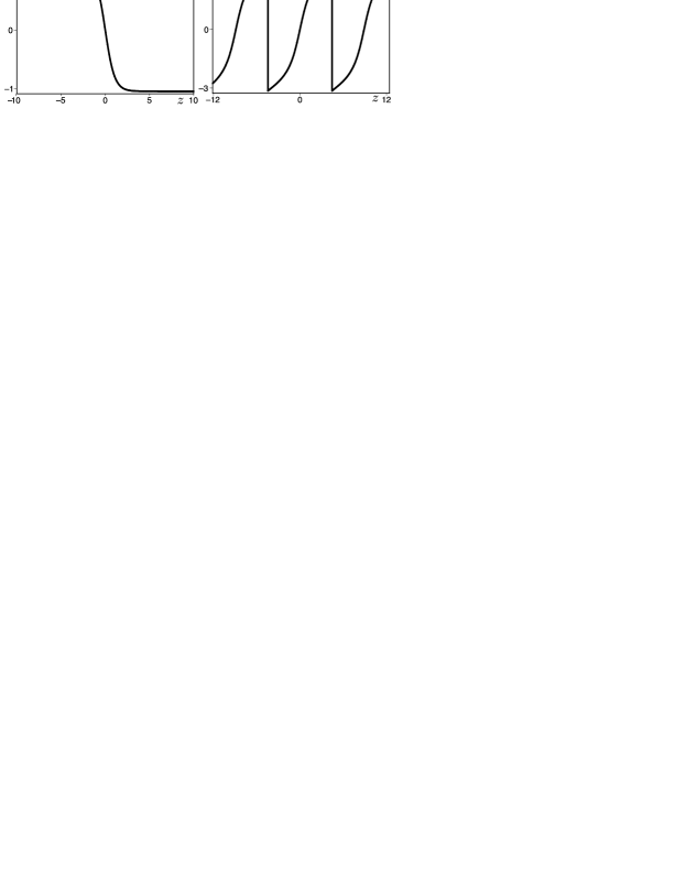
Figure 5: Solution (37) of equation (36) at a) $\gamma=1$, $\sigma=-2$ and $z_{0}=0$; b) $\sigma=1$, $\gamma=1/2$ and $z_{0}=0$.

Thus, we find one–parametric solutions family of (36). When $\gamma\sigma^{2}>1$ solution (37) is a smooth and monotonic function, while in the case of $\gamma\sigma^{2}<1$ is is a periodic discontinuous function. We demonstrate plots of solution (37) for the both cases $\gamma\sigma^{2}>1$ and $\gamma\sigma^{2}<1$ in Fig.5.

In this section we have constructed three new examples of integrable Liénard equations with the help of Theorems 1–3. We have obtained closed–form expressions for the general solutions of these equations. We have also demonstrated that we can find explicit expressions for the one–parametric families of analytical solutions of the Liénard equation by means of Corollaries 1–3. We believe that all solutions obtained in this section are new.

4 Conclusion

In this work have studied connections between the Liénard equation and equation of the Painlevé–Gambier type. We have considered all subcases of equation (1) that belong to the Painlevé–Gambier classification. We have demonstrated that some of these equation can be linearized via the generalized Sundman transformations, and, therefore do not lead to new integrability conditions for the Liénard equation. On the other hand, the rest Painlevé integrable subcases of equation (1) give us new criteria for integrability of the Liénard equation. The case of equation VII was considered in [15], while connection between equation (1) and equations II, V and XVII from the Painlevé–Gambier classification have been considered in the present work. As a result, we have found three new criteria for the integrability of the Liénard equation. We have demonstrated applications of our approach by constructing general analytical solutions of three new integrable Liénard equations. We have also proposed an approach for finding one–parameter families of closed form analytical solutions of the Liénard equation. We have shown that in some cases we can effectively find one–parametric families of analytical solutions of the Liénard equation.

5 Acknowledgments

This research was partially supported by grant for the state support of young Russian scientists 6624.2016.1 and by the grant for the state support of scientific schools 6748.2016.1.

References

- [1] J. Guckenheimer, P. Holmes, Nonlinear Oscillations, Dynamical Systems, and Bifurcations of Vector Fields, Springer New York, New York, NY, 1983.
- [2] A.A. Andronov, A.A. Vitt, A.A. Khaikin, Theory of Oscillators, Dover Publications, New York, 2011.
- [3] V.F. Zaitsev, A.D. Polyanin, Handbook of Exact Solutions for Ordinary Differential Equations, Chapman and Hall/CRC, Boca Raton, 2002.
- [4] M. Lakshmanan, S. Rajasekar, Nonlinear dynamics : integrability, chaos, and patterns, Springer, Heidelberg, 2003.
- [5] G. Villari, On the qualitative behaviour of solutions of Liénard equation, J. Differ. Equ. 67 (1987) 269–277.
- [6] L. Perko, Differential Equations and Dynamical Systems, Springer Verlag, New York, 2006.
- [7] M.C. Depassier, J. Mura, Variational approach to a class of nonlinear oscillators with several limit cycles, Phys. Rev. E. 64 (2001) 056217.
- [8] T. Carletti, G. Villari, A note on existence and uniqueness of limit cycles for Liénard systems, J. Math. Anal. Appl. 307 (2005) 763 773.
- [9] G. Bluman, A.F. Cheviakov, M. Senthilvelan, Solution and asymptotic/blow-up behaviour of a class of nonlinear dissipative systems, J. Math. Anal. Appl. 339 (2008) 1199 1209.
- [10] S.N. Pandey, P.S. Bindu, M. Senthilvelan, M. Lakshmanan, A group theoretical identification of integrable cases of the Liénard–type equation . I. Equations having nonmaximal number of Lie point symmetries, J. Math. Phys. 50 (2009) 082702.
- [11] S.N. Pandey, P.S. Bindu, M. Senthilvelan, M. Lakshmanan, A group theoretical identification of integrable equations in the Liénard–type equation . II. Equations having maximal Lie point symmetries, J. Math. Phys. 50 (2009) 102701.
- [12] V.K. Chandrasekar, M. Senthilvelan, M. Lakshmanan, On the complete integrability and linearization of certain second-order nonlinear ordinary differential equations, Proc. R. Soc. A Math. Phys. Eng. Sci. 461 (2005) 2451–2476.
- [13] W. Nakpim, S.V. Meleshko, Linearization of Second-Order Ordinary Differential Equations by Generalized Sundman Transformations, Symmetry, Integr. Geom. Methods Appl. 6 (2010) 1 11.
- [14] S. Moyo, S.V. Meleshko, Application of the generalised Sundman transformation to the linearisation of two second-order ordinary differential equations, J. Nonlinear Math. Phys. 18 (2011) 213 236.
- [15] N.A. Kudryashov, D.I. Sinelshchikov, On the criteria for integrability of the Liénard equation, Appl. Math. Lett. 57 (2016) 114–120.
- [16] S.C. Mancas, H.C. Rosu, Integrable dissipative nonlinear second order differential equations via factorizations and Abel equations, Phys. Lett. A. 377 (2013) 1434–1438.
- [17] T. Harko, F.S.N. Lobo, M.K. Mak, A class of exact solutions of the Liénard-type ordinary nonlinear differential equation, J. Eng. Math. 89 (2014) 193–205.
- [18] N.A. Kudryashov, D.I. Sinelshchikov, Analytical solutions of the Rayleigh equation for empty and gas-filled bubble, J. Phys. A Math. Theor. 47 (2014) 405202.
- [19] N.A. Kudryashov, D.I. Sinelshchikov, Analytical solutions for problems of bubble dynamics, Phys. Lett. A. 379 (2015) 798–802.
- [20] N.A. Kudryashov, D.I. Sinelshchikov, On the connection of the quadratic Lienard equation with an equation for the elliptic functions, Regul. Chaotic Dyn. 20 (2015) 486 496.
- [21] M. Sabatini, On the period function of , J. Differ. Equ. 196 (2004) 151–168.
- [22] G. Gubbiotti, M.C. Nucci, Quantization of quadratic Liénard–type equations by preserving Noether symmetries, J. Math. Anal. Appl. 422 (2015) 1235–1246.
- [23] E.L. Ince, Ordinary differential equations, Dover, New York, 1956.