Observational Evidence of Magnetic Reconnection for Brightenings and Transition Region Arcades in IRIS observations

Abstract

By using a new method of forced-field extrapolation, we study the emerging flux region AR 11850 observed by the Interface Region Imaging Spectrograph (IRIS) and Solar Dynamical Observatory (SDO). Our results suggest that the bright points (BPs) in this emerging region have responses in lines formed from the upper photosphere to the transition region, with a relatively similar morphology. They have an oscillation of several minutes according to the Atmospheric Imaging Assembly (AIA) data at 1600 and 1700 Å . The ratio between the BP intensities measured in 1600 Å  and 1700 Å  filtergrams reveals that these BPs are heated differently. Our analysis of the Helioseismic and Magnetic Imager (HMI) vector magnetic field and the corresponding topology in AR11850 indicates that the BPs are located at the polarity inversion line (PIL) and most of them related with magnetic reconnection or cancelation. The heating of the BPs might be different due to different magnetic topology. We find that the heating due to the magnetic cancelation would be stronger than the case of bald patch reconnection. The plasma density rather than the magnetic field strength could play a dominant role in this process. Based on physical conditions in the lower atmosphere, our forced-field extrapolation shows consistent results between the bright arcades visible in slit-jaw image (SJI) 1400 Å and the extrapolated field lines that pass through the bald patches. It provides a reliable observational evidence for testing the mechanism of magnetic reconnection for the BPs and arcades in emerging flux region, as proposed in simulation works.

1 Introduction

Prevalent energy releases can occur in the solar atmosphere in a large range of scales from solar flares to small energy release events. Solar flares have been extensively studied (Parker, 1981; Phillips, 1991; Schrijver, 2009; Milligan, 2015; Janvier et al., 2015, and the references therein) as it is the most energetic phenomenon and frequently accompanied by coronal mass ejection, which may influence the space weather and even our earth. The small-scale energy release events happen more frequently and have been named as micro- and nanoflares, bright points (BPs), blinkers. They have been observed by different instruments (Schmieder et al., 1995; Parnell et al., 2002; Aschwanden, 2004) in different wavelengths from visible to soft X-ray. They have important impacts on the heating mechanisms of the solar atmosphere. Such events take place in different atmospheric layers from the photosphere to the corona (Harrison, 1997; Berger et al., 2007; Chandrashekhar et al., 2013), and ubiquitous in active regions, quiet Sun and coronal holes (Shimizu, 1995; Zhang et al., 2001; Kamio et al., 2011). With the ground-based and space telescopes, photospheric BPs are often studied to investigate the condition of the convective flows in and below the photosphere (Feng et al., 2013; Jafarzadeh et al., 2014; Yang et al., 2015, 2016; Ji et al., 2016a, b). These flows are widely accepted to be the ultimate source of the energy; coronal BPs as well as coronal loops are also frequently discussed (Li et al., 2013; Zhang et al., 2014; Alipour & Safari, 2015; Chesny et al., 2015; Mou et al., 2016) as they were thought to be the most potential candidates for coronal heating.

In fact, the energy coming from the solar convection region heats the solar atmosphere through the stressing of the magnetic field lines, and manifests itself as waves and current sheets leading to reconnection (see review in Schmieder et al., 2014). The anomalous high temperature in the corona is one manifestation of this process. The temperature of the chromosphere is not as high as that of the corona because of its higher density. Hence, we need to study the atmosphere as an entirety to understand the heating process (such as Schmieder, 1997; Schmieder et al., 2004; Li et al., 2007; Zhao & Li, 2012), and particularly pay attention to the phenomena happening in the chromosphere and transition region.

Previous diagnostic work have been done on the small-scale energy release events in this interface region (Schmieder, 1997; Pariat et al., 2004, 2006, 2007; Tian et al., 2010; Chen & Ding, 2010; Brosius & Holman, 2010; Brosius, 2013; Leiko & Kondrashova, 2015), with limited wavelengths, resolution, sensitivity or observation time. The recently launched Interface Region Imaging Spectrograph (IRIS, De Pontieu et al., 2014b), which provided images and spectrum with considerably high temporal and spatial resolution, has opened a new window for investigating the small-scale energy release events in the interface region. Some impressive findings (Hansteen et al., 2014; De Pontieu et al., 2014a; Tian et al., 2014; Peter et al., 2014; Rouppe van der Voort et al., 2015; Vissers et al., 2015) and more specific works (Huang et al., 2014; Martínez-Sykora et al., 2015; Kim et al., 2015; Park et al., 2016; Skogsrud et al., 2016; Brooks et al., 2016) have been introduced. Most of them have focused on the transition region loops, torsional motions, solar spicules, bright grains, explosive events, Ellerman bombs (EBs) and the hot bombs which turn out to be the analogies of EBs (Tian et al., 2016). Such phenomena have been studied in details, including their spectrum, temperature, morphology, lifetime. However, no direct analysis of the related magnetic field has been done yet.

Although it is still not clear whether waves or reconnection play a dominant role in heating the solar atmosphere, it is well accepted that the solar plasma, which is ionized due to the high temperature, is highly coupled to the magnetic field. An evidence is the dominance of the structured magnetic field associated with the inhomogeneities of the emission in the solar corona. Hence, the magnetic topology, especially the special features such as null points, separatrix surfaces, separators as well as quasi-separatrix layers (QSLs), is considered to be important for studying the atmospheric heating. The magnetic field associated with the BPs can be achieved thanks to the availability of high quality vector magnetograms, and the advanced reconstruction method of the coronal force-free magnetic field. As a result, the coronal BPs and the associated magnetic features have been well studied in the tenuous and highly ionized coronal plasma where magnetic reconnection can occur easily (such as Zhang et al., 2012; Ning & Guo, 2014). A bunch of work have made some approximations in studying the interface brightenings with the photospheric magnetic fields (such as Pariat et al., 2007; Li & Ning, 2012; Jiang et al., 2015; Li & Zhang, 2016)

Several simulation work have studied the heating of the solar atmosphere from convection zone to the corona (Potts et al., 2007; Pariat et al., 2009; Jiang et al., 2010, 2012; Ni et al., 2015a, b, 2016), yet the investigation of the magnetic features in real physical conditions is considerably insufficient in the lower atmosphere. Schmieder & Aulanier (2003) discussed the linear force-free-field (LFFF) method in emerging active region and also its limitation. In Feng et al. (2007), they even pointed out the inadequacy of the LFFF extrapolation in the corona by comparing with their reliable coronal loop reconstruction. Pariat et al. (2004, 2006) studied the emergence of a magnetic flux tube and the heating during this process. Their LFFF extrapolation result suggests that the impulsive heating may happen not only at the locations of the bald patches but also at the footpoints and along the field lines that passing through these bald patches. Valori et al. (2012) focused on the entire process of the flux emergence, from the first appearance of the magnetic signature in the photosphere, until the formation of the main bipole of the active region. They adopted the non-linear force-free-field (NLFFF) extrapolation based on the magneto-frictional method to construct the three-dimensional magnetic field in the emerging flux region. Hong et al. (2016) studied a micro-flare in the chromosphere with the spectra measured by the New Solar Telescope (NST; Goode et al., 2003) at Big Bear Solar Observatory (BBSO) and extrapolated magnetic fields from Helioseismic and Magnetic Imager (HMI; Scherrer et al., 2012) with a NLFFF approach (Wheatland, 2004; Wiegelmann & Inhester, 2010). However, the force-free assumption inside these work is probably not consistent with the physical conditions in the lower atmosphere. In fact, all the NLFFF extrapolation methods encounter more or less the following difficulties in the investigation of the magnetic field in the interface region: Firstly, the plasma in the lower atmosphere is partially ionized and with high density. In the chromosphere the plasma beta fluctuates a lot and can be either above or bellow 1, which makes it much more sophisticated in analyzing the initiation and driving mechanism of the reconnection. Secondly, the magnetic field in the lower atmosphere, which is filled with short and low-lying loops, is much more complex than in the corona. Thirdly, the Lorentz force is nonzero, hence the force-free assumption used in the extrapolation is invalid. Therefore in this paper we applied a new forced-field extrapolation method based on a magnetohydrodynamic (MHD) relaxation method developed recently by Zhu et al. (2013), which has already shown their advantages in Zhu et al. (2016).

In this work, we investigate the magnetic topology of the BPs happening in between an emerging flux region observed by the Solar Dynamical Observatory (SDO) and IRIS. A new method of the forced-field extrapolation is adopted (Zhu et al., 2013). This paper is organized as follows: the observations are introduced in Section 2 and extrapolation in Section 3. We discuss our results and make conclusions in Section 4.

2 Observations

2.1 Overview of the Active Region

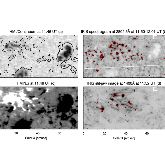
Figure 1: Emerging flux with BPs observed by IRIS and HMI in AR11850 on September 24, 2013. (a) HMI continuum image, showing the location of the spots. Contours (values equal $\pm 200$ G, solid lines for negative polarity and dash-doted lines for positive polarity) of the vertical magnetic field are overlaid. (b) Spectrogram between 11:50 and 12:01 UT in Mg II h line wing (2803.5 +1 Å) with red contours overlain; (c) Vertical magnetic field component map at 11:46 UT in the photosphere, the maximum and minimum value of the magnetic field is $\pm 200$ G. (d) SJI at Si IV 1400 Å with red contours overlain; We present negative color for panel (b) and (d) that the black color shows high intensity and white color for low intensity. Same formula is used for Figure 2 (a) and (c), Figure 3 (a), Figure 12 and Figure 13.

NOAA AR11850 appears at the location of E$24^{\circ}$N$8^{\circ}$ on September 24, 2013. It is an emerging flux region and consists of three dispersed spots (Figure 1a). The AR11850 has been captured by telescopes both in the space and on the ground, which makes it a suitable region for analyzing the successive heating of the solar atmosphere. There are many BPs appearing in between this active region, Peter et al. (2014) studied four of them and considered them as ”hot explosions”; Grubecka et al. (2016) made statistics on the compact BPs observed in this region.

The Atmospheric Imaging Assembly (AIA) instrument (Lemen et al., 2012) onboard SDO satellite obtains full-disk images in UV and EUV wavelengths and monitors the atmosphere from the chromosphere to the corona with high spatial resolution (0.6 arcsec per pixel) and continuous temporal coverage. The IRIS mission (De Pontieu et al., 2014b) obtains UV spectra and images of the chromosphere and transition region, with a spectral resolution of respectively $\approx 26$ and $\approx 52$ mÅ according to the wavelength range, and a spatial resolution of 0.33 – 0.4 arcsec for the images. IRIS observed AR11850 with a FOV of 141 arcsec $\times$ 175 arcsec for the raster and 166 arcsec $\times$ 175 arcsec for the image.

The cadence of the slit-jaw images (SJI) in the Si IV 1400 Å filter is 12 seconds. Images using the rasters can be obtained in 20 minutes (first interval is 11:44 – 12:04 UT and second interval 15:39 –15:59 UT) on September 24, 2013. We will mainly use the SJI 1400 Å observed at 11:52 UT and the spectrogram in the Mg II h line wing at 2803.5 +1 Å  scanned from 11:50 to 12:01 UT in the first time interval of observations and covering only the emerging flux region.

2.2 Observations by IRIS and SDO/AIA

Since we are mostly interested in the initial phase of the emerging process when the flux tubes pass through the lower solar atmosphere, especially through the photosphere, we mainly investigate the observations of this emerging flux region in UV wavelengths.

For a context of AR 11850, we present the HMI continuum intensity and photospheric magnetogram in Figure 1 (a) and (c) to show the magnetic configuration in this region. The images of different UV wavelengths are shown in Figure 1 (b) and (d), in IRIS spectrogram at 2804.5 Å from 11:50 to 12:01 UT and SJI 1400 Å at 11:52 UT, with approximated formation temperatures of $10^{4.0}$ and $10^{4.8}$ kelvin, respectively. In both UV images, there are several well-pronounced BPs in the moss between the magnetic polarities, which are outlined by red contours. A bunch of plasma loops can also be recognized in 1400 Å image, which might correspond to the arch filament system (AFS) in H$\alpha$ (refer to Grubecka et al., 2016), with their feet rooted at some of the aforementioned BPs. In SJI 1400 Å  there are 19 bright points between magnetic polarities in this active region with a threshold value of 20 times above the $I_{smean}$, while in 2804.5 Å  there are 50 bright points with a threshold value of 1.6 times above the $I_{mmean}$. The values of $I_{smean}$ and $I_{mmean}$ represent the mean intensity in a relatively quiet region indicated by the rectangular white box in Si IV and Mg II images, respectively.

Most of the intense BPs that appear in 2804.5 Å have a counterpart in SJI 1400 Å  although they are not outlined by red contours due to the contour level that we have selected to avoid mixing of BPs and bright loops. In the magnetogram, we have increased the contrast to enhance the small-scaled dipoles between the spots. The relationship between the bright points and magnetic dipoles will be studied in detail later.

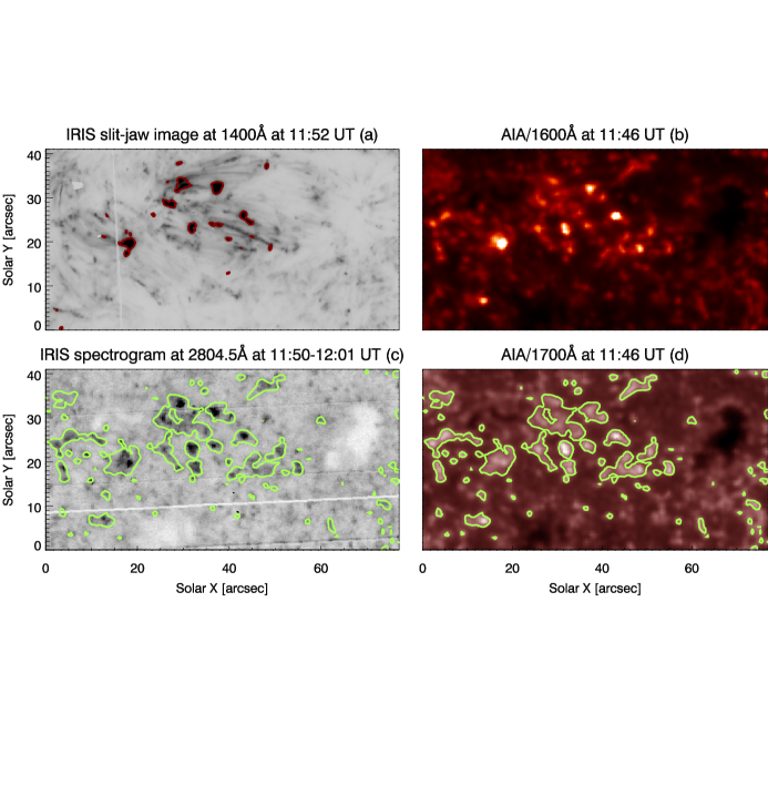
Figure 2: Emerging flux with BPs observed by IRIS and AIA in AR11850. (a) SJI at Si IV 1400 Å with contours of the bright points; (b) Intensity image at 1600 Å  (c) Spectrogram between 11:50 and 12:01 UT in Mg II h wing (2803.5 +1 Å) with contour of 1600 Å intensity image overlain; (d) Intensity image at 1700 Å with contour of 1600 Å intensity image overlain.

The UV images at other wavelengths, such as AIA 1600 and 1700 Å  are shown in Figure 2. The 1700 Å emission (UV continuum) forms around the temperature minimum region of $10^{3.7}$ kelvin, while the 1600 Å emission contains UV emission like 1700 Å and also the emission of C IV line 1548 Å formed in the transition region temperature. Complementary images from IRIS are also displaced here. These four images reveal the atmosphere response to the magnetic flux emergence from photosphere to the transition region. The images from the different satellites are coaligned through the alignment of specific features. The contours of 1600 Å intensity image are overlaid on IRIS 2804.5 Å and AIA 1700 Å images. It implies that all the images are coaligned quite well. A large number of BPs can be identified in the moss between the spots in 1600 and 1700 Å images.

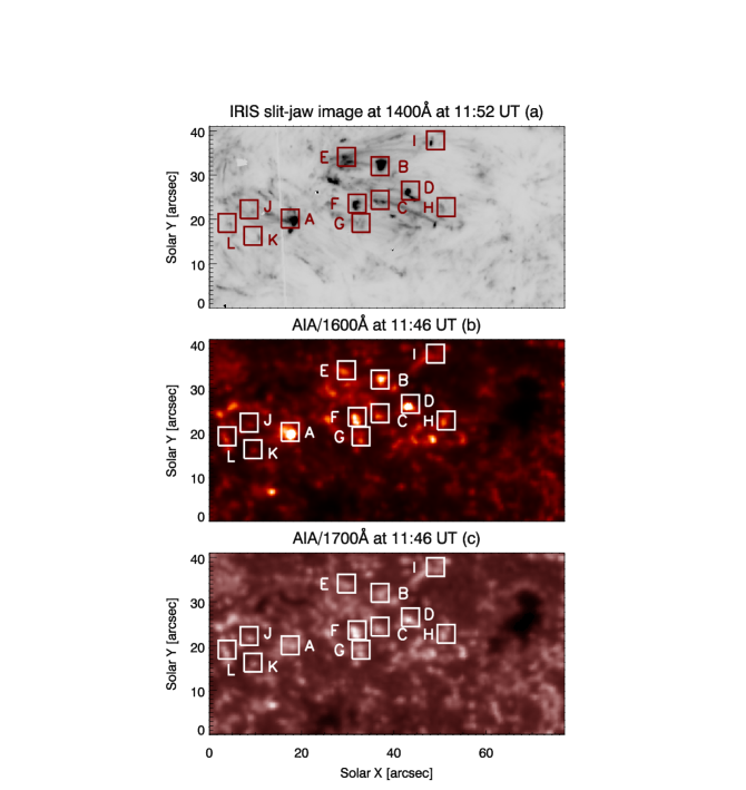
Figure 3: Intensity images of AR11850 at different wavelengths at 11:52 UT and at 11:46 UT. The square boxes select twelve BPs (A to L) that are studied in detail in the paper.

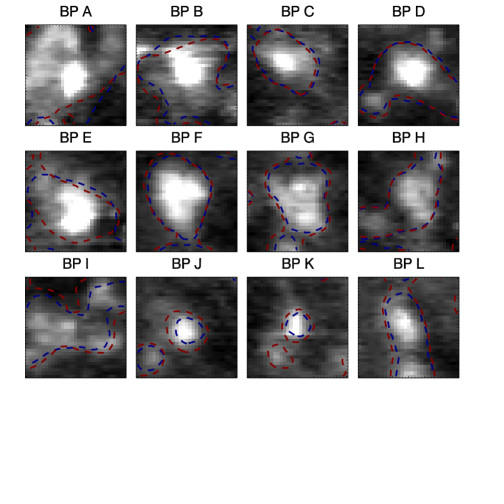
Figure 4: Intensity images for BPs A – L in Mg II h wing (2803.5 +1 Å). The AIA 1600 Å (blue) and 1700 Å (red) contours are overlaid.

Among these BPs, we selected several brightest ones A-I by visual inspection of their brightness in IRIS 1400 Å and present them with rectangular box in Figure 3. All the selected BPs have their counterparts in AIA 1600 Å and 1700 Å. This result suggests that the BPs are heated in the atmosphere from the photosphere to the transition region. In order to compare the morphology of these BPs, we overlay the contours of AIA 1600 Å (2.2 times above the mean value) and AIA 1700 Å (1.4 times above the mean value) on the spectrogram of 2804.5 Å for every single BP in Figure 4. We notice that most of the BPs have a similar morphology, with a more diffuse shape in the AIA observations. As mentioned in Vissers et al. (2015) and Tian et al. (2016), the BPs observed in Mg II line wing commonly have a counterpart in the wings of H$\alpha$ like the EBs. It indicates that the BPs marked in the boxes maybe associated with EBs.

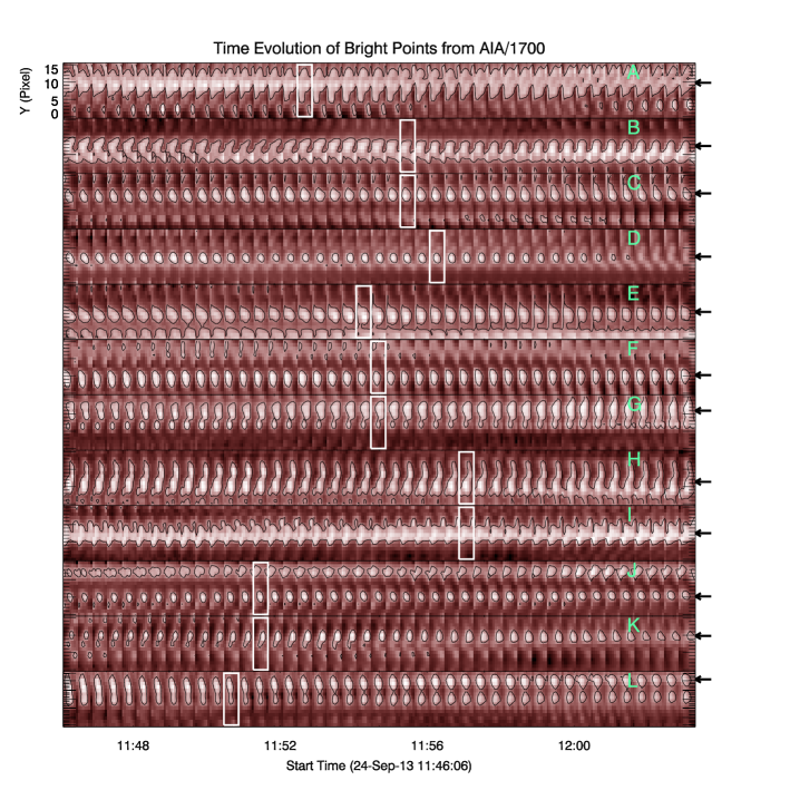
Figure 6: Temporal evolution of the brightness in 1700 Å of twelve selected BPs. The boxes indicate the time of the BP spectra obtained by IRIS during the raster.

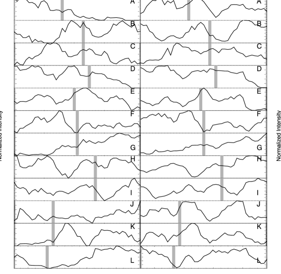
Figure 7: Intensity curves in 1600 Å and 1700 Å of twelve selected BPs versus time. The grey rectangular regions label the IRIS scanning time of the BPs, respectively

We present the evolution of selected BPs in 1600 Å in Figure 5 and in 1700 Å in Figure 6. The images record the BPs evolution for 16 minutes from 11:46 UT to 12:04 UT. The black contours outline the BPs in this rectangular region and the black arrow points out the specific one that we are interested in. The morphology of BP A and B seems to be different in 1600 Å and 1700 Å  while the others are similar. The shape of these BPs always changes during the 18 minutes. The white rectangular boxes show the times when the slit of IRIS scans through these BPs. We calculated the intensity ratio between 1600 Å and 1700 Å at these specific times (Table 1). All ratios are greater than unity except for BP I. These ratios imply that there is a contribution of C IV emission in the BPs. The more the ratio is greater than unit, the more the contribution comes from C IV. Hence, we could find that the C IV emission contributes much more in BPs A , B and E, less for C, D, F and almost no for the others (G to L). It means that the temperature of the BPs A to F is higher than that of the others. This is consistent with the results of Grubecka et al. (2016), who found signatures in Si IV spectra only for the BPs corresponding to the classes of A, B, D. From the temporal evolution of the above BPs, we obtain the intensity curves in 1600 and 1700 Å shown in Figure 7. The BPs appear to have an oscillation of several minutes, just like the jets. This is probably due to the recurrent reconnection modulated by the plasma motion and releases energy quasi-periodically. This scenario has been supported by the theoretical (Santos & Büchner, 2007; Pariat et al., 2010) and observational (Madjarska et al., 2003; Ugarte-Urra et al., 2004; Doyle et al., 2006; Yang et al., 2011; Zhang et al., 2012; Guo et al., 2013; Samanta et al., 2015; Innes et al., 2016) work.

2.3 Observations by SDO/HMI

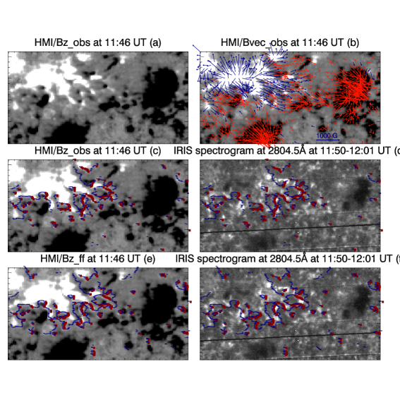
Figure 8: Magnetograms of the photosphere at 11:46 UT and IRIS spectrogram between 11:50 UT and 12:01 UT. (a) Vertical magnetic field component at the photosphere from observations; (b) Vector magnetogram at photosphere. The background is vertical magnetic field and the blue and red arrows represent the horizontal magnetic field with positive and negative vertical magnetic field, respectively; (c) Same as (a) but with PIL (blue dots) and bald patches (red dots) overlain; (d) Spectrogram at Mg II 2804.5 Å with bald patches from observations located; (e) Vertical magnetogram at photosphere from forced field extrapolation with PIL (blue dots) and bald patches (red dots) overlaid; (f) Spectrogram at Mg II 2804.5 Å with bald patches from extrapolation located.

As the magnetic field has intimate relation with the phenomenon happened in the solar atmosphere, our study also included the analysis of the vector magnetic field at the photosphere as well as the extrapolated field based on it. The vector magnetic field is provided by the HMI onboard SDO, with a spatial resolution of 0.5 arcsec per pixel and a temporal resolution of 12 minutes. We present the images of the vertical component B_z and the vector B_vec of the observed magnetic field in Figure 8 (a, b, c), and display the bottom layer of the extrapolated magnetic field in Figure 8 (e). We see magnetic fields with mixed polarities between the spots. These are the preferential places for a specific bald patch topology structure (red points in Figure 8 (c – f)). This conception dates back to Titov et al. (1993). The authors emphasized a place on the polarity inversion line (PIL) at the photosphere where magnetic field line threading through it horizontally from negative to positive polarity, and named it as ’Bald Patch’. It relates to a serpentine field line when the flux tube emerging from the convective region to the solar atmosphere (Fan, 2001a, b; Pariat et al., 2009). Similar structure has also been found in the low altitude atmosphere and can be identified as ’magnetic dip’ refer to Pariat et al. (2004). Cool and dense material often deposite in these dips. Such location as well as its related BP separatrix has been found to be preferential place for reconnection when proper surface flows are involved. Such reconnection is responsible for the EBs and brightening loops in many studies of observation and simulation (Pariat et al., 2009). In the spectral observations, blueshift and redshift of spectral lines (such as Si IV, C II, Mg II) associated with the bidirectional flows are frequently recognized around these places (Cheng et al., 2015). The comparison of the images of 2804.5 Å  overlaid by bald patches derived from observation and from extrapolation, shows a similar distribution of the bald patches in the field of view (Figure 8 (d, f)). It means that the extrapolation correctly retrieves the magnetic field structures.

The calculation of bald pathes or magnetic dips in 3D volume is based on the magnetic field in 3D. It is provided by the forced-field extrapolation described in the next section.

3 Forced-Field Extrapolation

To investigate the relationship of the BPs and loops with the associated magnetic field, we extrapolated the magnetic field from Space-weather HMI Active Region Patch (SHARP) Cylindrical Equal Area (CEA) data of SDO/HMI. The forced-field extrapolation code is described in Zhu et al. (2013) and computes the magnetic field by solving full MHD equations using a kind of relaxation method. The initial state comprises a plane-parallel multilayered hydrostatic model (Fan, 2001a), embedded with a potential magnetic field (Sakurai, 1982) determined by the normal component of the vector magnetogram. The outflow condition is applied for both sides and upper boundaries. At the lower boundary the normal component of the magnetic field is fixed, while the transverse field is slowly changed from the initial condition to the observed field. This is called the ”stress and relax” approach (Roumeliotis, 1996) which drives the system to evolve. Finally, the Lorentz Force near the photosphere can be balanced by the pressure gradient and plasma gravity, and the forced equilibrium of the entire region can be reached. Our extrapolation is done on the initial size of the grid, e.g. 1 grid equal 0.5 arcsec, with a domain of 328 $\times$ 248 $\times$ 160 grid.

Then we calculated the locations of bald patches referring to the equation in Pariat et al. (2004):

$$B_{z}=0\quad and\quad{\bm{B}}\bullet{\nabla}{B_{z}}>0$$ (1)

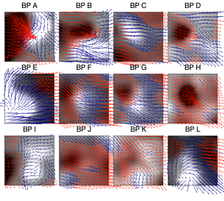
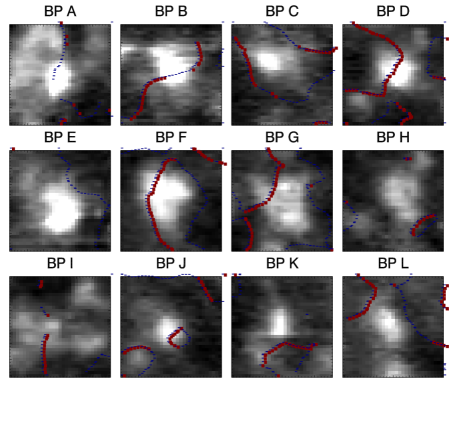
Figure 9: Upper three rows show the vector magnetic field of selected BPs and lower rows show the locations of PIL (blue dots) and bald patches (red dots) on the IRIS Mg II h wing (2803.5 +1 Å) images.

the magnetic topologies of BPs A – L in detail are illustrated in Figure 9. In our study, the BPs A, B and I are located above the magnetic PIL where magnetic flux cancelation is dominant, the BPs D, F, G, J have consistent locations with their corresponding bald patches. However, we don’t see the consistency of the locations between the BPs C, H, K, L and their corresponding bald patches. The BP E is located over the PIL, without bald patch or cancelation topology. In our later study, we find that BPs C, E, H, K, L are at the footpoints of bald patch related separatrix layers. The relevant bald patches are located far away from the BPs.

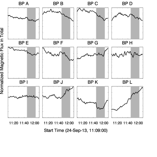
Figure 10: The curves show the evolution of the normalized magnetic flux for the selected BPs from 11:09 UT to 12:09 UT. They sum the positive and modulus of the negative magnetic flux. The grey rectangular regions give the time range of the AIA observations and the scanning period of the IRIS in our work.

The temporal evolution of the magnetic flux of these BPs is shown in Figure 10. All these curves start from 11:09 UT and end at 12:09 UT. They cover the time range of the AIA and IRIS observations indicated by the grey rectangular region (11:46 UT to 12:04 UT) in each panel. The curves of BPs A, B and D, F display a continuous decrease, while the curves of BPs I and G, J show a temporary one during the observation (in the grey region). It manifests that magnetic cancelation and reconnection, which are responsible for the plasma heating, have happened either continuously or temporarily. Apparently, the continuous cancelation or reconnection would produce stronger heating effect than the temporary one according to Table 1. The rest curves describe the local condition of the magnetic flux, and are meaningless for understanding the BPs C, E, H, K, L that are related with separatrix layer footpoints. The different magnetic situation of the BPs is clearly shown in Figure 11.

Considering that the BPs A, B, D and I correspond to bombs 3, 4, 1 and 2 in Peter et al. (2014) respectively, the bomb 1 (BP D) seems to be related with bald patch reconnection while the other three bombs 2 (BP I), 3 (BP A), 4 (BP B) are produced by flux cancelation. In addition, Grubecka et al. (2016) studied the formation height of the same BPs and listed their result in their Table 3. The altitude of hot spots A – E ranges from 75 – 900 km from a 1D solar atmosphere model with the radiative transfer code of Heinzel (1995). The formation height of A, B is relatively higher than D, which could indicate that the cancelation reconnection happened a little higher than the BP reconnection. It is surprising to detect that the ”hot explosions” (BPs A, B and I ) of Peter et al. (2014) correspond principally to the flux cancellation region rather than a bald patch region like the bomb 1 (point D in our analysis). Their large emission values indicate that reconnection by flux cancellation lead to stronger heating than in bald patch configuration.

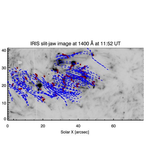
Figure 12: Overview of magnetic field line connectivity in AR11850. Red dots mark the locations of bald patches; Blue field lines display magnetic field lines passing through the corresponding bald patches obtained by a forced-field extrapolation.

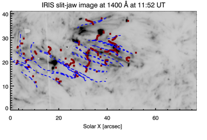
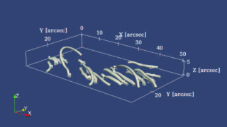
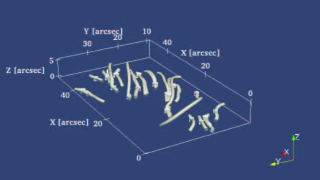
Figure 13: Selected magnetic field lines in AR11850. Upper panel: top view; Bottom panels: side views. The red dots (in the upper panel) and the white dots (in the bottom panels) mark the locations of bald patch.

The extrapolated field lines lying between the polarities and passing through the bald patches which are labeled as red points are overplotted on the IRIS SJI 1400 Å in Figure 12 and the upper panel of Figure 13. Figure 12 shows an overview of the field lines in this AR, while in Figure 13 we only selected several representatives for clarity. These field lines have diverse lengths but with a coherent direction going from the positive to the negative polarities. Most of the brightening loops appearing in 1400 Å have good correspondence with the magnetic field lines in profile. Hence, we suggest that the brightening loops in the interface layer of this active region are at least partially contributed by the reconnection along the bald patch separatrices.

We also extract these field lines and exhibit their side views in the bottom panels of Figure 13. The spatial distribution of the sea-serpent structures is prominent. Most of these structures have relatively low altitude, while some higher field lines have a height of less than 3.5 Mm. The white points mark the locations of the bald patch that the field lines passing through. It manifests that the bald patch often connect two arcades, one is lower and shorter and the other is higher and longer, just like the case from MHD model in Aulanier et al. (1998).

4 Discussion and Conclusion

In this work, we have investigated an active region during its emerging phase. In this phase, there are plenty of BPs that appear in between this region, i.e. in the moss, which indicates that the atmosphere above has been heated. Hence, it is meaningful to study the properties of the BPs for understanding the heating of the upper atmosphere under the following two questions: 1) To what extent does the emerging flux heat the atmosphere above? and 2) At which location does the heating become more effective?

This active region has been observed by the Multichannel Subtractive Double Pass spectrograph (MSDP) in the Meudon Solar Tower on the ground and IRIS as well as SDO in the space. These telescopes provide the images of this region from photosphere to the corona, and also the spectra of the transition region which has already been analyzed by Peter et al. (2014) and Grubecka et al. (2016). Here we selected IRIS SJI at 1400 Å and spectrogram in Mg II h line wing at 2804.5 Å , AIA 1600 Å and 1700 Å to analyze the atmosphere response to the emerging flux. Our results demonstrate that the BPs that appear in the IRIS SJI 1400 Å have their counterparts in other wavelengths (formed at the minimum temperature) that we mentioned above, and most of them have similar morphology. Referring to the formation temperatures of these spectral lines, we suggest that the emerging flux could heat the solar atmosphere from the upper photosphere to the transition region.

We also investigate the temporal evolution of these BPs in AIA 1600 and 1700 Å. They always exist during the period of around 20 minutes. However, the curve of intensity evolution shows a periodic variation of several minutes, which could be probably due to the periodic reconnection. According to the scanning time of the IRIS raster, we determined the moments when the raster scanning through these BPs (labeled as white rectangular boxes in Figure 5 and 6) and calculated the intensity ratio between AIA 1600 Å and 1700 Å at these moments. The results suggest that some BPs, such as A to F, have more contribution from C IV line, i.e. from higher temperature plasma while the others do not.

As the heating only happens at particular sites, e.g. the BP sites, it means that the energy release only occurs under special conditions. For understanding the non-uniform heating effect, we have studied the properties of these BPs in detail to see how they are heated and why the heating effects are different. The magnetic configuration and the magnetic flux evolution at the corresponding locations suggest that BPs A, B and I are consistent with the magnetic cancelation scenario, BPs D, F, G, J appear to have magnetic bald patch topology, and BPs C, E, H, K, L are located at the footpoints of the bald patch related separatrix layers. The magnetic field separatrix layers are volume structures at where the magnetic connectivity changes and current sheet can easily form (Low, 1987). Considering the contribution of the C IV line in different BPs, our results indicate that the bald patch reconnection may have weaker heating effect than the magnetic cancelation, and the continuous cancelation or reconnection may have stronger heating effect than the temporary one.

According to the simulation work of Ni et al. (2016), the level of the heating effect depends on the local plasma $\beta$, which is directly proportional with plasma density and inversely proportional to magnetic field strength. Their results show that low $\beta$ magnetic reconnection process is associated with high temperature events and high $\beta$ with low temperature events. In our situation, more materials would be deposited at the bald patch locations than in cancelation regions. Supposing the magnetic field under these two conditions is of the same order, we suggest that our observational analyzes support the theoretical results.

Besides the BP sites, energy release also happens at some bright arcade structures. According to previous studies based on the LFFF or NLFFF extrapolations, or MHD simulation, these structures are suspected to be related to the reconnection happened at the serpentine field lines that passing through the bald patches (Pariat et al., 2007; Valori et al., 2012; Pariat et al., 2009). With our extrapolation result, we obtain the corresponding serpentine field lines and suggest that these lines have good accordance with the bright arcades in between the emerging region. This fact confirms the conclusions of previous works from an observational aspect, that is when the new flux emerges, it may have some difficulty in passing through the photosphere and becomes horizontal at the sub-surface as the pressure height changes. It can only continue the emergence until the reconnection happens at its magnetic dips as well as its separatrix surface under suitable photospheric flows. The bright arcades visible in SJI 1400 Å indicate that probable reconnection between the emerging flux and the overlying magnetic flux occurs in current layers at QSLs, as suggested in the simulation work of Pariat et al. (2009).

In summary, we have studied the BPs and transition region arcades in an emerging flux region. Using our forced-field extrapolation, we find observational evidence of magnetic reconnection for these structures. This is the first time for the extrapolation method, which considering the physical condition in the lower atmosphere, to be used for investigating the local heating events.

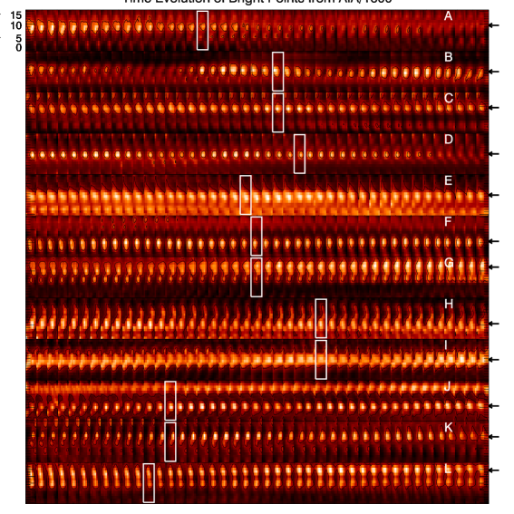
Figure 5: Temporal evolution of the brightness in 1600 Å of the twelve selected BPs. The boxes indicate the time of the BP spectra obtained by IRIS during the raster.

Table 1: Intensity ratio of 1600 Å to 1700 Å of the selected bright points A-I

Bright Point	Ratio	Bright Point	Ratio	Bright Point	Ratio
A(Bomb 3)	1.29	E	1.25	I(Bomb 2)	0.95
B(Bomb 4)	1.52	F	1.19	J	1.04
C	1.13	G	1.04	K	1.02
D(Bomb 1)	1.16	H	1.03	L	1.06

Figure 11: Sketch for the magnetic conditions of the BPs A to L.

References

- Alipour & Safari (2015) Alipour, N., & Safari, H. 2015, ApJ, 807, 175
- Aschwanden (2004) Aschwanden, M. J. 2004, Physics of the Solar Corona. An Introduction (Praxis Publishing Ltd)
- Aulanier et al. (1998) Aulanier, G., Démoulin, P., Schmieder, B., Fang, C., & Tang, Y. H. 1998, Sol. Phys., 183, 369
- Berger et al. (2007) Berger, T. E., Rouppe van der Voort, L., & Löfdahl, M. 2007, ApJ, 661, 1272
- Brooks et al. (2016) Brooks, D. H., Reep, J. W., & Warren, H. P. 2016, ApJ, 826, L18
- Brosius (2013) Brosius, J. W. 2013, ApJ, 777, 135
- Brosius & Holman (2010) Brosius, J. W., & Holman, G. D. 2010, ApJ, 720, 1472
- Chandrashekhar et al. (2013) Chandrashekhar, K., Krishna Prasad, S., Banerjee, D., Ravindra, B., & Seaton, D. B. 2013, Sol. Phys., 286, 125
- Chen & Ding (2010) Chen, F., & Ding, M. D. 2010, ApJ, 724, 640
- Cheng et al. (2015) Cheng, X., Ding, M. D., & Fang, C. 2015, ApJ, 804, 82
- Chesny et al. (2015) Chesny, D. L., Oluseyi, H. M., Orange, N. B., & Champey, P. R. 2015, ApJ, 814, 124
- De Pontieu et al. (2014a) De Pontieu, B., Rouppe van der Voort, L., McIntosh, S. W., et al. 2014a, Science, 346, 1255732
- De Pontieu et al. (2014b) De Pontieu, B., Title, A. M., Lemen, J. R., et al. 2014b, Sol. Phys., 289, 2733
- Doyle et al. (2006) Doyle, J. G., Popescu, M. D., & Taroyan, Y. 2006, A&A, 446, 327
- Fan (2001a) Fan, Y. 2001a, ApJ, 546, 509
- Fan (2001b) —. 2001b, ApJ, 554, L111
- Feng et al. (2007) Feng, L., Inhester, B., Solanki, S. K., et al. 2007, ApJ, 671, L205
- Feng et al. (2013) Feng, S., Deng, L., Yang, Y., & Ji, K. 2013, Ap&SS, 348, 17
- Goode et al. (2003) Goode, P. R., Denker, C. J., Didkovsky, L. I., Kuhn, J. R., & Wang, H. 2003, Journal of Korean Astronomical Society, 36, S125
- Grubecka et al. (2016) Grubecka, M., Schmieder, B., Berlicki, A., et al. 2016, A&A, 593, A32
- Guo et al. (2013) Guo, Y., Démoulin, P., Schmieder, B., et al. 2013, A&A, 555, A19
- Hansteen et al. (2014) Hansteen, V., De Pontieu, B., Carlsson, M., et al. 2014, Science, 346, 1255757
- Harrison (1997) Harrison, R. A. 1997, Sol. Phys., 175, 467
- Heinzel (1995) Heinzel, P. 1995, A&A, 299, 563
- Hong et al. (2016) Hong, J., Ding, M. D., Li, Y., et al. 2016, ApJ, 820, L17
- Huang et al. (2014) Huang, Z., Madjarska, M. S., Xia, L., et al. 2014, ApJ, 797, 88
- Innes et al. (2016) Innes, D. E., Bučík, R., Guo, L.-J., & Nitta, N. 2016, Astronomische Nachrichten, 337, 1024
- Jafarzadeh et al. (2014) Jafarzadeh, S., Cameron, R. H., Solanki, S. K., et al. 2014, A&A, 563, A101
- Janvier et al. (2015) Janvier, M., Aulanier, G., & Démoulin, P. 2015, Sol. Phys., 290, 3425
- Ji et al. (2016a) Ji, K., Jiang, X., Feng, S., et al. 2016a, Sol. Phys., 291, 357
- Ji et al. (2016b) Ji, K.-F., Xiong, J.-P., Xiang, Y.-Y., et al. 2016b, Research in Astronomy and Astrophysics, 16, 009
- Jiang et al. (2015) Jiang, F., Zhang, J., & Yang, S. 2015, PASJ, 67, 40
- Jiang et al. (2010) Jiang, R. L., Fang, C., & Chen, P. F. 2010, ApJ, 710, 1387
- Jiang et al. (2012) Jiang, R.-L., Fang, C., & Chen, P.-F. 2012, ApJ, 751, 152
- Kamio et al. (2011) Kamio, S., Curdt, W., Teriaca, L., & Innes, D. E. 2011, A&A, 529, A21
- Kim et al. (2015) Kim, Y.-H., Yurchyshyn, V., Bong, S.-C., et al. 2015, ApJ, 810, 38
- Leiko & Kondrashova (2015) Leiko, U. M., & Kondrashova, N. N. 2015, Advances in Space Research, 55, 886
- Lemen et al. (2012) Lemen, J. R., Title, A. M., Akin, D. J., et al. 2012, Sol. Phys., 275, 17
- Li & Ning (2012) Li, D., & Ning, Z. 2012, Ap&SS, 341, 215
- Li et al. (2013) Li, D., Ning, Z. J., & Wang, J. F. 2013, New A, 23, 19
- Li et al. (2007) Li, H., Sakurai, T., Ichimito, K., et al. 2007, PASJ, 59, S643
- Li & Zhang (2016) Li, T., & Zhang, J. 2016, A&A, 589, A114
- Low (1987) Low, B. C. 1987, ApJ, 323, 358
- Madjarska et al. (2003) Madjarska, M. S., Doyle, J. G., Teriaca, L., & Banerjee, D. 2003, A&A, 398, 775
- Martínez-Sykora et al. (2015) Martínez-Sykora, J., Rouppe van der Voort, L., Carlsson, M., et al. 2015, ApJ, 803, 44
- Milligan (2015) Milligan, R. O. 2015, Sol. Phys., 290, 3399
- Mou et al. (2016) Mou, C., Huang, Z., Xia, L., et al. 2016, ApJ, 818, 9
- Ni et al. (2015a) Ni, L., Kliem, B., Lin, J., & Wu, N. 2015a, ApJ, 799, 79
- Ni et al. (2015b) Ni, L., Lin, J., Mei, Z., & Li, Y. 2015b, ApJ, 812, 92
- Ni et al. (2016) Ni, L., Lin, J., Roussev, I. I., & Schmieder, B. 2016, ArXiv e-prints, arXiv:1611.01746
- Ning & Guo (2014) Ning, Z., & Guo, Y. 2014, ApJ, 794, 79
- Pariat et al. (2010) Pariat, E., Antiochos, S. K., & DeVore, C. R. 2010, ApJ, 714, 1762
- Pariat et al. (2004) Pariat, E., Aulanier, G., Schmieder, B., et al. 2004, ApJ, 614, 1099
- Pariat et al. (2006) —. 2006, Advances in Space Research, 38, 902
- Pariat et al. (2009) Pariat, E., Masson, S., & Aulanier, G. 2009, ApJ, 701, 1911
- Pariat et al. (2007) Pariat, E., Schmieder, B., Berlicki, A., et al. 2007, A&A, 473, 279
- Park et al. (2016) Park, S.-H., Tsiropoula, G., Kontogiannis, I., et al. 2016, A&A, 586, A25
- Parker (1981) Parker, E. N. 1981, Geophysical and Astrophysical Fluid Dynamics, 18, 332
- Parnell et al. (2002) Parnell, C. E., Bewsher, D., & Harrison, R. A. 2002, Sol. Phys., 206, 249
- Peter et al. (2014) Peter, H., Tian, H., Curdt, W., et al. 2014, Science, 346, 1255726
- Phillips (1991) Phillips, K. J. H. 1991, Vistas in Astronomy, 34, 353
- Potts et al. (2007) Potts, H. E., Khan, J. I., & Diver, D. A. 2007, Sol. Phys., 245, 55
- Roumeliotis (1996) Roumeliotis, G. 1996, ApJ, 473, 1095
- Rouppe van der Voort et al. (2015) Rouppe van der Voort, L., De Pontieu, B., Pereira, T. M. D., Carlsson, M., & Hansteen, V. 2015, ApJ, 799, L3
- Sakurai (1982) Sakurai, T. 1982, Sol. Phys., 76, 301
- Samanta et al. (2015) Samanta, T., Banerjee, D., & Tian, H. 2015, ApJ, 806, 172
- Santos & Büchner (2007) Santos, J. C., & Büchner, J. 2007, Astrophysics and Space Sciences Transactions, 3, 29
- Scherrer et al. (2012) Scherrer, P. H., Schou, J., Bush, R. I., et al. 2012, Sol. Phys., 275, 207
- Schmieder (1997) Schmieder, B. 1997, in Lecture Notes in Physics, Berlin Springer Verlag, Vol. 489, European Meeting on Solar Physics, ed. G. M. Simnett, C. E. Alissandrakis, & L. Vlahos, 139
- Schmieder et al. (2014) Schmieder, B., Archontis, V., & Pariat, E. 2014, Space Sci. Rev., 186, 227
- Schmieder & Aulanier (2003) Schmieder, B., & Aulanier, G. 2003, Advances in Space Research, 32, 1875
- Schmieder et al. (2004) Schmieder, B., Rust, D. M., Georgoulis, M. K., Démoulin, P., & Bernasconi, P. N. 2004, ApJ, 601, 530
- Schmieder et al. (1995) Schmieder, B., Shibata, K., van Driel-Gesztelyi, L., & Freeland, S. 1995, Sol. Phys., 156, 245
- Schrijver (2009) Schrijver, C. J. 2009, Advances in Space Research, 43, 739
- Shimizu (1995) Shimizu, T. 1995, PASJ, 47, 251
- Skogsrud et al. (2016) Skogsrud, H., Rouppe van der Voort, L., & De Pontieu, B. 2016, ApJ, 817, 124
- Tian et al. (2010) Tian, H., Potts, H. E., Marsch, E., Attie, R., & He, J.-S. 2010, A&A, 519, A58
- Tian et al. (2016) Tian, H., Xu, Z., He, J., & Madsen, C. 2016, ApJ, 824, 96
- Tian et al. (2014) Tian, H., DeLuca, E. E., Cranmer, S. R., et al. 2014, Science, 346, 1255711
- Titov et al. (1993) Titov, V. S., Priest, E. R., & Demoulin, P. 1993, A&A, 276, 564
- Ugarte-Urra et al. (2004) Ugarte-Urra, I., Doyle, J. G., Madjarska, M. S., & O’Shea, E. 2004, A&A, 418, 313
- Valori et al. (2012) Valori, G., Green, L. M., Démoulin, P., et al. 2012, Sol. Phys., 278, 73
- Vissers et al. (2015) Vissers, G. J. M., Rouppe van der Voort, L. H. M., Rutten, R. J., Carlsson, M., & De Pontieu, B. 2015, ApJ, 812, 11
- Wheatland (2004) Wheatland, M. S. 2004, Sol. Phys., 222, 247
- Wiegelmann & Inhester (2010) Wiegelmann, T., & Inhester, B. 2010, A&A, 516, A107
- Yang et al. (2011) Yang, S., Zhang, J., Li, T., & Liu, Y. 2011, ApJ, 732, L7
- Yang et al. (2015) Yang, Y., Ji, K., Feng, S., et al. 2015, ApJ, 810, 88
- Yang et al. (2016) Yang, Y., Li, Q., Ji, K., et al. 2016, Sol. Phys., 291, 1089
- Zhang et al. (2001) Zhang, J., Kundu, M. R., & White, S. M. 2001, Sol. Phys., 198, 347
- Zhang et al. (2014) Zhang, Q. M., Chen, P. F., Ding, M. D., & Ji, H. S. 2014, A&A, 568, A30
- Zhang et al. (2012) Zhang, Q. M., Chen, P. F., Guo, Y., Fang, C., & Ding, M. D. 2012, ApJ, 746, 19
- Zhao & Li (2012) Zhao, J., & Li, H. 2012, Research in Astronomy and Astrophysics, 12, 1681
- Zhu et al. (2013) Zhu, X. S., Wang, H. N., Du, Z. L., & Fan, Y. L. 2013, ApJ, 768, 119
- Zhu et al. (2016) Zhu, X. S., Wang, H. N., Du, Z. L., & He, H. 2016, ApJ, 826, 51