Observational View of Magnetic Fields in Active Galactic Nuclei Jets

Abstract

According to the currently favored picture, relativistic jets in active galactic nuclei (AGN) are launched in the vicinity of the black hole by magnetic fields extracting energy from the spinning black hole or the accretion disk. In the past decades, various models from shocks to magnetic reconnection have been proposed as the energy dissipation mechanism in the jets. This paper presents a short review on how linear polarization observations can be used to constrain the magnetic field structure in the jets of AGN, and how the observations can be used to constrain the various emission models.

1 Introduction

Active galactic nuclei (AGN) are among the most extreme objects in the universe. They are the centers of distant galaxies hosting a supermassive black hole, billions of times the mass of the Sun. About 10% of AGN produce collimated, relativistic outflows or plasma jets that shine brightly over the entire electromagnetic spectrum from radio to gamma-ray energies. The formation and stability of these jets are not yet fully understood. It is believed that energy is extracted from the central black hole by large-scale magnetic fields ([Blandford & Znajek 1977]) while rotating inner regions of the accretion disk form an outflowing wind that helps to collimate the jet ([Blandford & Payne 1982]). In this picture, the jet is launched as a magnetically dominated outflow with strong magnetic fields accelerating the flow to relativistic velocities. General relativistic magnetohydrodynamic simulations show that the efficiency of the jet generation can be very high if the black hole is threaded by a dynamically important magnetic field ([Tchekhovskoy et al. 2011]).

While the simulations suggest that the jets are likely highly magnetized near the black hole, their composition and magnetic field structure in the parsec scales, where they produce most of the emission, is much less clear. A link between the magnetic fields near the black hole and the parsec-scale jets was established by [Zamaninasab et al. 2014, Zamaninasab et al. (2014)] who showed that there is a correlation between the magnetic flux of the jet and the accretion disk luminosity, as predicted by the magnetically arrested disk (MAD) model ([Tchekhovskoy et al. 2011]). This result illustrates how studying the emission regions in the parsec-scale jets may help us gain knowledge about the jet formation processes.

One of the main open questions is the nature of the emission region. Traditionally, the flaring behavior of AGN jets has been well explained by shock-in-jet models, especially in the radio bands (e.g., [Hughes et al. 1985, Marscher & Gear 1985]). These models assume the jet to be kinetically dominated at parsec scales. Shock models struggle to explain the very fast variability detected at high-energy gamma-ray bands, and models involving magnetic reconnection have been invoked to explain the high-energy emission (e.g., [Giannios et al. 2009]). In this case the jet flow should be magnetically dominated, although recent particle-in-cell simulations show that even in reconnection models, the magnetic field and particle energies can be in equipartition at the emission region ([Sironi et al. 2015]).

Another major open question is the structure of the magnetic field at the emission site. According to the simulations, the magnetic field is helical close to the black hole but whether it preserves its order in the parsec scales is debated upon. For example, in the model of [Marscher et al. 2008, Marscher et al. (2008)], the magnetic field is helical at the acceleration and collimation zone of the jet but gets disrupted and turbulent beyond a standing shock in the jet. Polarization observations of some jets, however, indicate that the magnetic field could be helical even on the parsec scales (e.g., [Asada et al. 2002, Gabuzda et al. 2004, Hovatta et al. 2012]). Figure 1 shows an example adapted from [Hovatta et al. 2012, Hovatta et al. (2012)].

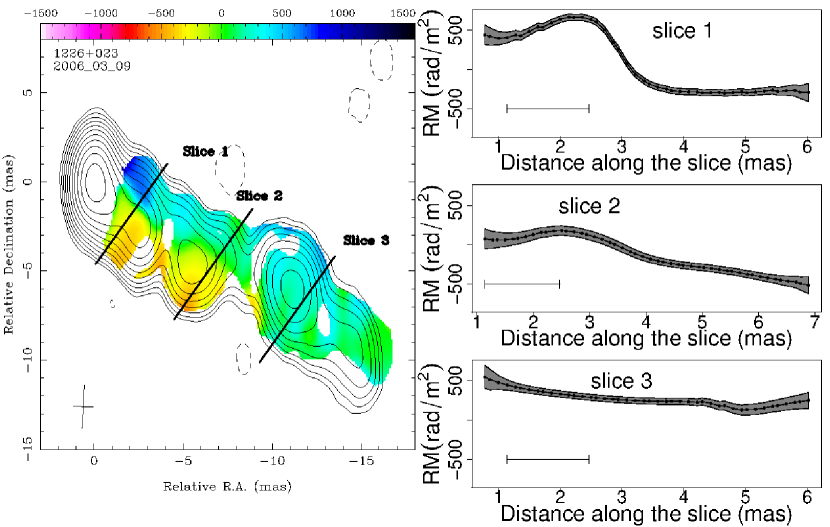
Figure 1: Faraday rotation map of 3C 273 obtained with the VLBA at 8 - 15 GHz. A rotation measure gradient is seen extending the full length of the jet. This can be interpreted as a signature of a helical magnetic field. Figure adapted from [Hovatta et al. 2012, Hovatta et al. (2012)].

In this contribution, I will discuss how linear polarization observations in the radio and optical bands can be used to constrain jet emission models and the magnetic field structure of the jets. This is not intended as a comprehensive review of all possible models, but more to give some examples on how observations are used to study magnetic fields in AGN jets.

2 Polarization observations

The optical and radio emission of AGN jets is synchrotron emission, which is intrinsically highly polarized. In an optically thin emission region with a uniform magnetic field, the polarization degree is up to 70% (e.g., [Pacholczyk 1970]), although such high polarization degree values are not typically seen in AGN jets in the radio (e.g., [Aller et al. 2003, Lister & Homan 2005]) or optical (e.g., [Angel & Stockman 1980, Pavlidou et al. 2014]) bands. This has been taken as evidence for disordered magnetic fields. The emission in AGN jets is often described with the Stokes parameters I (for total intensity), Q and U (for linear polarization) and V (for circular polarization). I will only discuss linear polarization here. Using the Stokes parameters, the polarization degree and the electric vector position angle (EVPA) can be defined as $m=(\sqrt{Q^{2}+U^{2}})/I$ and EVPA$=1/2\tan^{-1}(U/Q)$. In the simplest case, in an optically thin jet, the polarization position angle is perpendicular to the magnetic field direction and one can use the EVPA observations to infer the direction of the magnetic field. However, one should note that in relativistic jets viewed at a small angle to the line of sight of the observer, the situation is more complicated ([Lyutikov et al. 2005]).

Another way to obtain information about magnetic fields in blazar jets is via Faraday rotation observations. When synchrotron radiation passes through magnetized plasma, Faraday rotation of the EVPAs proportional to the line-of-sight magnetic field and electron density occurs (e.g. [Burn 1966]). In the simplest case, the effect can be described by a linear dependence between the observed electric vector position angle (EVPA; $\chi_{\mathrm{obs}}$) and wavelength squared ($\lambda^{2}$), given by

$$\chi_{\mathrm{obs}}=\chi_{0}+0.81\int n_{e}\mathbf{B}\cdot\mathbf{\mathrm{d}l}=\chi_{0}+\mathrm{RM}\lambda^{2},$$ (1)

where $\chi_{0}$ is the intrinsic EVPA and RM is the rotation measure (in rad/m²), related to the electron density $n_{e}$ of the plasma (in cm^-3) and the magnetic field component $\mathbf{B}$ (in $\mu$G) along the line of sight (in parsecs). The RM can thus be estimated by observing the EVPA at different frequencies. This will give us information on the line-of-sight component of the magnetic field. For example, if the rotation measure is positive, the magnetic field is coming towards the observer, and if negative it is going away from the observer. Therefore it was suggested that a gradient in a Faraday rotation measure transverse to the jet direction could reveal helical magnetic field structures ([Blandford 1993]).

3 Constraining emission models through polarimetry

Polarization observations of AGN jets in the radio and optical bands have been conducted since the 1970s (see e.g., [Saikia & Salter 1988] for a review). At the same time, a large number of theoretical models were developed to explain the total intensity and polarization observations of AGN jets (e.g, [Jones & O’Dell 1977, Blandford & Königl 1979, Laing 1980]). In the 1980s it was suggested that most of the radio variability, especially in the cm-band, are due to shocks in the relativistic jets where the magnetic field is predominantly turbulent ([Hughes et al. 1985, Marscher & Gear 1985, Jones et al. 1985]).

The field of polarization modeling has received a new boost since an exciting connection to high-energy gamma-ray emission was found ([Marscher et al. 2008]). A rotation in the optical polarization angle was coincident with an ejection of a new very long baseline interferometry (VLBI) component from the core, and a very-high-energy (VHE; $>$ 100 GeV) detection of the source BL Lac by the MAGIC telescope. A further connection between the optical polarization and gamma-ray flares was suggested in two quasars 3C 279 ([Abdo et al. 2010]) and PKS 1510-089 ([Marscher et al. 2010, Aleksić et al. 2014]). In both of these the optical polarization angle was seen to rotate by more than 180 degrees over a course of 20 to 50 days during which a sharp gamma-ray flare was observed. Following all these observations, a number of new models have been published in the last years (e.g., [Marscher 2014, Zhang et al. 2014, Hughes et al. 2015, Zhang et al. 2015]). I will go through some of these models with the emphasis on the observations that can be used to constrain them.

3.1 Turbulence in the jets

Turbulent magnetic field produces stochastic variations to the polarization angle and degree ([Jones et al. 1985, Marscher 2014]), such as an EVPA rotation of any length, typically accompanied by a low polarization degree. The challenge in constraining these types of models is the stochastic nature of the variations so that it is not possible to fit the individual light curves ([Marscher 2014]). Instead, one should observe a large number of objects and compare the statistical properties of the variations with the turbulent models.

To study the connection between high-energy emission and optical polarization in a statistical manner, the RoboPol program was initiated in 2013 ([Pavlidou et al. 2014]). The RoboPol instrument is mounted on the 1.3-m telescope in Skinakas Observatory in Crete, where the observing season lasts from April until November. During its first three observing seasons, RoboPol observed about 100 AGN twice per each week in search of optical polarization angle rotations. The main goal was to study the differences in gamma-ray detected and non-detected objects, and to search for a connection between rotations and flaring behavior.

RoboPol has detected 40 optical polarization angle rotations during the first three observing seasons, tripling the number of known rotations ([Blinov et al. 2015, Blinov et al. 2016a, Blinov et al. 2016b]). Comparing the rotations with random walk simulations showed that while stochastic variability for any individual rotation could not be ruled out, it was highly unlikely that all of them would be of random walk origin. [Kiehlmann et al. 2016, Kiehlmann et al. (2016)] suggested that the smoothness of the rotation could be used as an additional indicator when comparing the rotations with random walk models. They also illustrated the importance of good sampling in polarization observations by revealing how additional data changed the rotation reported by [Abdo et al. 2010, Abdo et al. (2010)] in the quasar 3C 279.

Figure 2 shows an example of a EVPA rotation in the source 1ES 1727+502 studied in [Hovatta et al. 2016, Hovatta et al. (2016)]. Based on random walk simulations, conducted in the same manner as in [Kiehlmann et al. 2016, Kiehlmann et al. (2016)], a stochastic origin for the rotation cannot be excluded.

Figure 2: Polarization degree and EVPA of 1ES 1727+502 in 2014 observed with RoboPol and the Nordic Optical Telescope (NOT). The EVPA shows a rotation of nearly 150 degrees in about 60 days. Figure adapted from [Hovatta et al. 2016, Hovatta et al. (2016)].

3.2 Emission in a helical field

A rotation in the polarization angle could also be due to an emission feature tracing a magnetic field in the jet as suggested by [Marscher et al. 2008, Marscher et al. (2008)] and [Marscher et al. 2010, Marscher et al. (2010)]. In this model, the magnetic field in the jet is helical in the acceleration and collimation zone, which is probed by the optical band, and a rotation is seen when the emission feature moves along the magnetic field. The rotation may be accompanied by flaring in other bands when the emission feature reaches a standing shock in the jet.

Another alternative is a shock moving down a jet with a helical field, in which case the EVPA rotation would be due to light travel time effects when parts of the shock are seen at different times ([Zhang et al. 2014]). This model was used to successfully fit the EVPA rotation in the quasar 3C 279 ([Zhang et al. 2015]), although one should bear in mind the caveat that with the additional data from [Kiehlmann et al. 2016, Kiehlmann et al. (2016)], the rotation was not as long as originally presented by [Abdo et al. 2010, Abdo et al. (2010)].

Whether the magnetic field in the jet is helical, especially in regions beyond the acceleration and collimation zone, is still unclear. As explained in Sect. 2, observations of a Faraday rotation measure gradient across the jet could be an indication of such a field. First signatures of a helical magnetic field were observed in the quasar 3C 273 using multifrequency very long baseline array (VLBA) observations ([Asada et al. 2002, Zavala & Taylor 2005]). Many more claims of such gradients have been made (e.g., [Gabuzda et al. 2004]) but the issue has been controversial due to the limited resolution across the jets in blazars ([Taylor & Zavala 2010]).

In [Hovatta et al. 2012, Hovatta et al. (2012)], we performed Monte Carlo simulations to quantify the significance of the rotation measure gradients in the large sample of parsec-scale jets in the MOJAVE (Monitoring of Jets in Active galactic nuclei with VLBA Experiments) sample. Our observations confirmed the gradient in 3C 273 (see Fig. 1), and we also found significant gradients in three other quasars. In [Zamaninasab et al. 2013, Zamaninasab et al. (2013)] we modelled the gradient of the quasar 3C 454.3 using a magnetic field with both helical and turbulent components. In the other two sources, the gradient span only over a small portion of the jet and detailed modeling was not possible.

Nowadays performing simulations to quantify the significance of the gradients is a common practice (e.g., [Murphy & Gabuzda 2013]) and the number of significant gradients has steadily increased (e.g., [Gabuzda et al. 2015]). However, rotation measure gradients can also arise from changes in the density of the Faraday rotating material (e.g. [Gómez et al. 2011]) so that detailed modeling of the gradients should be done in order to confirm that they are indeed due to helical fields. It is also unclear whether the helical field is within the jet or in a sheath layer around the jet because Faraday rotation is a propagation effect originating in the plasma outside the emission region.

3.3 Shock in a jet

As stated earlier, shock-in-jet models have been successful in reproducing the observed flaring especially in the radio bands. Typically, radiative transfer simulations are generated to estimate the parameters of the shocks (e.g. [Hughes et al. 2011, Hughes et al. 2015]) and these are then compared with observations at multiple bands ([Aller et al. 2014]). For example, as shown by [Hughes et al. 2015], the polarization degree and range of EVPA values can be used to constrain the magnetic field geometry and jet orientation, while total intensity behavior is indistinguishable in different models.

Interestingly, although the magnetic field is assumed to be predominantly turbulent, in some cases an ordered field component (possibly helical) could also be present ([Aller et al. 2016]). This supports the findings of e.g., [Zamaninasab et al. 2013, Blinov et al. 2015, Zamaninasab et al. (2013), Blinov et al. (2015)], and [Kiehlmann et al. 2016, Kiehlmann et al. (2016)], who also suggest that there are both turbulent and ordered magnetic field components / deterministic variations in the jets.

3.4 Magnetic reconnection

Magnetic reconnection (see [Kagan et al. 2015] for a review) is a new hot topic in the field. It was originally invoked to explain the fast high-energy variability of blazars through the jet-in-jet model ([Giannios et al. 2009]). In the recent years, particle-in-cell simulations have evolved significantly, and it is now possible to reliably simulate the complicated structure of the reconnection layer (e.g., [Sironi et al. 2015]). While the reconnection models can already be compared to total intensity variability of the sources ([Petropoulou et al. 2016]), there are no explicit models for the polarized emission.

[Zhang et al. 2015, Zhang et al. (2015)] stated that the EVPA swing in the 2009 flare of 3C 279 was reproduced by a model that “favors magnetic energy dissipation process during the flare” because the magnetic field strength was seen to decrease when the total intensity increased. However, this model did not yet include detailed comparisons to a specific reconnection model. Considering the growing interest in the magnetic dissipation models, it is likely that in the next few years more detailed models with observational predictions will become available.

3.5 Statistical trends

From the previous sections, it is clear that polarization observations can be used to constrain various types of emission models and the magnetic field structure in the jets. In order to generalize the findings in individual sources into the AGN jet population, a statistical approach must be used. This is what the RoboPol program aims for by observing a sample of about 100 sources with high cadence. RoboPol has found, for example, that any class of blazars from low to high synchrotron peaking objects can show rotations (see also [Jermak et al. 2016, Hovatta et al. 2016]). However, there seems to be a specific class of “rotators” that do so more often, and rotations are more common in the low spectral peaking objects ([Blinov et al. 2016b]).

The low synchrotron peaking objects also have higher optical polarization degree than the high-peaking objects ([Angelakis et al. 2016]), a trend that has also been seen in the smaller sample studied in [Jermak et al. 2016, Jermak et al. (2016)] and earlier in the radio band ([Lister et al. 2011]). These general trends can be explained with a simple, qualitative model where a shock moves down a jet, which has both helical and turbulent magnetic field components (see [Angelakis et al. 2016] for details). Any model put forward to explain the polarization behavior in individual flares, should also account for these general trends.

4 Future directions

One challenge in connecting the observations of magnetic fields to the theory of jet formation is that often the observations, especially in the radio bands, probe regions $10^{3}-10^{5}$ gravitational radii away from the black hole. Optical observations do not suffer from this restriction, but for example, Faraday rotation with $\lambda^{2}$ wavelength dependence, is not typically seen at optical wavelengths. A solution can be provided by going to millimeter-band observations, as demonstrated by [Martí-Vidal et al. 2015, Martí-Vidal et al. (2015)]. They used ALMA polarization observations to probe the Faraday rotation at the jet base of the lensed quasar PKS 1830-211, and found extremely high Faraday rotation of $10^{8}$rad/m², which is two orders of magnitude higher than previous observations in other sources (e.g., [Plambeck et al. 2014]). They inferred this as a signature of a very high magnetic field at the base of the jet, in support of magnetically launched jet models. Whether similar high RM values are a common property of quasars remains to be seen with future ALMA observations. Especially interesting will be future observations using ALMA as part of the global VLBI array, which may be able to spatially resolve the regions of high magnetic fields.

A major leap forward will come with the future X-ray polarization missions because the amount of polarization for different high-energy emission mechanisms in AGN jets, for example between leptonic and hadronic models, is very different ([Zhang & Böttcher 2013]), and X-ray polarization observations can be used to distinguish between the models.

5 Summary

Magnetic fields in AGN jets can be probed through polarization observations, which are most easily done at radio and optical bands. Modeling the polarization degree and position angle behavior can be used to test different blazar emission models, while Faraday rotation observations at radio, and now also in the millimeter bands, can be used to probe the line-of-sight magnetic field component. A statistical approach is favored when connecting the results to different AGN jet populations.

References

- [Abdo et al. 2010] Abdo, A. A., Ackermann, M., Ajello, M. et al. 2010, Nature, 463, 18
- [Aleksić et al. 2014] Aleksić, J., Ansoldi, S., Antonelli, L. A. et al. 2014 A&A, 569, 46
- [Aller et al. 2003] Aller, M. F., Aller, H. D. & Hughes, P. A. 2003, ApJ, 586, 33
- [Aller et al. 2014] Aller, M. F., Hughes, P. A., Aller, H. D. et al. 2014, ApJ, 791, 51
- [Aller et al. 2016] Aller, M. F., Hughes, P. A., Aller, H. D., et al. 2016, Galaxies, 4, 35
- [Angel & Stockman 1980] Angel, J. R. P. & Stockman, H. S. 1980, ARA&A, 18, 321
- [Angelakis et al. 2016] Angelakis, E., Hovatta, T., Blinov, D. et al. 2016 MNRAS, 463, 3365
- [Asada et al. 2002] Asada, K. Inoue, M., Uchida, Y., et al. 2002, PASJ, 54, L39
- [Blandford 1993] Blandford, R. 1993, in: M. Burgarella, M. Livio, & C. P. O’Dea (eds.) Astrophysical Jets, (Astrophysics and Space Science Library, Vol. 103; Cambridge: Cambridge Univ. Press), 15
- [Blandford & Königl 1979] Blandford, R. D. & Königl, A. 1979, ApJ, 232, 34
- [Blandford & Payne 1982] Blandford, R. D. & Payne, D. G. 1982, MNRAS, 199, 883
- [Blandford & Znajek 1977] Blandford, R. D. & Znajek, R. L. 1977, MNRAS, 179, 433
- [Blinov et al. 2015] Blinov, D., Pavlidou, V., Papadakis, I. et al. 2015, MNRAS, 453, 1669
- [Blinov et al. 2016a] Blinov, D., Pavlidou, V., Papadakis, I. E. et al. 2016a, MNRAS, 457, 2252
- [Blinov et al. 2016b] Blinov, D., Pavlidou, V., Papadakis, I. E. et al. 2016b, MNRAS, 462, 1775
- [Burn 1966] Burn, B. J. 1966, MNRAS, 133, 67
- [Gabuzda et al. 2015] Gabuzda D. C., Knuettel, S. & Reardon, B. 2015 MNRAS, 450, 2441
- [Gabuzda et al. 2004] Gabuzda, D. C., Murray, E., & Cronin, P. 2004, MNRAS, 351, L89
- [Giannios et al. 2009] Giannios, D., Uzdensky, D. A. & Begelman, M. C. 2009, MNRAS, 359, L29
- [Gómez et al. 2011] Gómez, J.-L., Roca-Sogorb, M., Agudo, I., et al. 2011, ApJ, 733, 11
- [Hovatta et al. 2012] Hovatta, T., Lister, M. L., Aller, M. F. et al. 2012, AJ, 144, 105
- [Hovatta et al. 2016] Hovatta, T., Lindfors, E., Blinov, D. et al. 2016 A&A, 596, 78
- [Hughes et al. 1985] Hughes, P. A., Aller, H. D. & Aller, M. F. 1985, ApJ, 298, 301
- [Hughes et al. 2011] Hughes, P. A., Aller, M. F., & Aller, H. D. 2011, ApJ, 735, 81
- [Hughes et al. 2015] Hughes, P. A., Aller, M. F., Aller, H. D. 2015, ApJ, 799, 207
- [Jermak et al. 2016] Jermak, H., Steele, I., Lindfors, E. et al. 2016, MNRAS, 462, 4267
- [Jones & O’Dell 1977] Jones, T. W. & O’Dell, S. 1977, ApJ, 215, 236
- [Jones et al. 1985] Jones, T. W., Rudnick, L., Aller, H. D. et al. 1985, ApJ, 290, 627
- [Kagan et al. 2015] Kagan, D., Sironi, L. Cerutti, B. & Giannios, D. 2015, Space Science Reviews, 191, 545
- [Kiehlmann et al. 2016] Kiehlmann, S., Savolainen, T., Jorstad, S. G., et al. 2016, A&A, 590, A10
- [Laing 1980] Laing, R. A. 1980, MNRAS, 193, 439
- [Lister & Homan 2005] Lister, M. L., & Homan, D. C. 2005, AJ, 130, 1389
- [Lister et al. 2011] Lister, M. L., Aller, M. F., Aller, H. D. et al. 2011, ApJ, 742, 27
- [Lyutikov et al. 2005] Lyutikov, M., Pariev, V. I., & Gabuzda, D. C. 2005, MNRAS, 360, 869
- [Marscher 2014] Marscher, A. P. 2014, ApJ, 780, 87
- [Marscher & Gear 1985] Marscher, A. P. & Gear, W. K. 1985, ApJ, 298, 114
- [Marscher et al. 2008] Marscher, A. P., Jorstad, S. G., D’Arcangelo, F. D. et al. 2008, Nature, 452, 966
- [Marscher et al. 2010] Marscher, A. P., Jorstad, S. G., Larionov, V. M. et al. 2010, ApJ, 710, L126
- [Martí-Vidal et al. 2015] Martí-Vidal, I., Muller, S., Vlemmings, W., Horellou, C., Aalto, S. 2015, Science, 348, 311
- [Murphy & Gabuzda 2013] Murphy E. & Gabuzda D. C. 2013, in The Inner-most Regions of Relativistic Jets and Their Magnetic Fields, EPJ Web of Conferences, Volume 61, id.07005
- [Pacholczyk 1970] Pacholczyk, A. G. 1970, Radio Astophysics, Nonthermal Processes in Galactic and Extragalactic Sources (San Francisco, CA: Freeman)
- [Pavlidou et al. 2014] Pavlidou, V., Angelakis, E., Myserlis, I. et al. 2014, MNRAS, 442, 1693
- [Petropoulou et al. 2016] Petropoulou, M., Giannios, D., Sironi, L. 2016, MNRAS, 462, 3325
- [Plambeck et al. 2014] Plambeck, R. L., Bower, G. C., Rao, R. et al. 2014, ApJ, 797, 66
- [Saikia & Salter 1988] Saikia, D. & Salter, C. 1988, Ann. Rev. in Astron. & Astrophys. , 26, 93
- [Sironi et al. 2015] Sironi, L., Petropoulou, M., & Giannios, D. 2015, MNRAS, 450, 183
- [Taylor & Zavala 2010] Taylor, G. B., & Zavala, R. T. 2010, ApJ, 722, L183
- [Tchekhovskoy et al. 2011] Tchekhovskoy, A., Narayan, R., McKinney, J. C. 2011, MNRAS, 418, L79
- [Zamaninasab et al. 2014] Zamaninasab, M., Clausen-Brown, E., Savolainen, T. & Tchekhovskoy, A. 2014, Nature, 510, 126
- [Zamaninasab et al. 2013] Zamaninasab, M., Savolainen, T., Clausen-Brown, E. et al. 2013, MNRAS, 436, 3341
- [Zavala & Taylor 2005] Zavala, R. T., & Taylor, G. B. 2005, ApJ, 626, L73
- [Zhang & Böttcher 2013] Zhang, H. & Böttcher, M. 2013, ApJ, 774, 18
- [Zhang et al. 2014] Zhang, H. Chen, X. & Böttcher, M. 2014, ApJ, 789, 66
- [Zhang et al. 2015] Zhang, H. Chen, X. & Böttcher, M. et al. 2015, ApJ, 804, 58