Orthogonal Polynomials related to ${g}$-fractions with missing terms

Abstract.

The purpose of the present paper is to investigate some structural and qualitative aspects of two different perturbations of the parameters of $g$-fractions. In this context the concept of gap $g$-fractions is introduced. While tail sequences of a continued fraction play a significant role in the first perturbation, Schur fractions are used in the second perturbation of the $g$-parameters that are considered. Illustrations are provided using Gaussian hypergeometric functions. Using a particular gap $g$-fraction, some members of the class of Pick functions are also identified.

1. Introduction

Given an arbitrary real sequence $\{g_{k}\}_{k=0}^{\infty}$, a continued fraction expansion of the form

$$\dfrac{1}{1}\begin{array}[]{cc}\\ $-$\end{array}\dfrac{(1-g_{0})g_{1}z}{1}\begin{array}[]{cc}\\ $-$\end{array}\dfrac{(1-g_{1})g_{2}z}{1}\begin{array}[]{cc}\\ $-$\end{array}\dfrac{(1-g_{2})g_{3}z}{1}\begin{array}[]{cc}\\ $-$\end{array}\cdots,\quad z\in\mathbb{C},$$ (1.9)

is called a $g$-fraction if the parameters $g_{j}\in[0,1]$, $j\in\mathbb{N}\cup\{0\}$. It terminates and equals a rational function if $g_{j}\in\{0,1\}$ for some $j\in\mathbb{N}\cup\{0\}$. If $0<g_{j}<1$, $j\in\mathbb{N}\cup\{0\}$, the $g$-fraction (1.9) still converges uniformly on every compact subsets of the slit domain $\mathbb{C}\setminus[1,\infty)$ (see [24, Theorem 27.5] and [11, Corollary 4.60]), and in this case, (1.9) will represent an analytic function, say $\mathcal{F}(z)$.

Such $g$-fractions are found having applications in diverse areas like number theory [21], dynamical systems [22], moment problems and analytic function theory [2, 12, 13]. In particular, [24, Theorem 69.2], the Hausdorff moment problem

$$\nu_{j}=\int_{0}^{1}\sigma^{j}d\nu(\sigma),\quad j\geq 0,$$

has a solution if and only if (1.9) corresponds to a power series of the form $1+\nu_{1}z+\nu_{2}z^{2}+\cdots$, $z\in\mathbb{C}\setminus[1,\infty)$. Further, the $g$-fractions have also been used to study the geometric properties of ratios of Gaussian hypergeometric functions as well as their $q$-analogues, (see the proofs of [12, Theorem 1.5] and [2, Theorem 2.2]). Among several such results, one of the most fundamental result concerning $g$-fraction is [24, Theorem 74.1] in which holomorphic functions having positive real part in $\mathbb{C}\setminus[1,\infty)$ are characterised. Precisely, $\mathrm{Re}(\sqrt{1+z}\,\,\mathcal{F}(z))$ is positive if and only if $\mathcal{F}(z)$ has a continued fraction expansion of the form (1.9). Moreover, $\mathcal{F}(z)$ has the integral representation

$$\mathcal{F}(z)=\int_{0}^{1}\dfrac{d\phi(t)}{1-zt},\quad z\in\mathbb{C}\setminus[1,\infty],$$

where $\phi(t)$ is a bounded non-decreasing function having a total increase 1.

Many interesting results are also available in literature if we consider subsets of $\mathbb{C}\setminus[1,\infty)$. For instance, let $\mathbb{K}$ be the class of holomorphic functions having a positive real part on the unit disk $\mathbb{D}:=\{z:|z|<1\}$. Such functions denoted by $\mathcal{C}(z)$ are called Carathéodory functions and have the Riesz-Herglotz representation [24, Theorem 73.1]

$$\mathcal{C}(z)=\int_{0}^{2\pi}\dfrac{e^{it}+z}{e^{it}-z}d\phi(t)+qi,$$

where $q$=$\mathrm{Im}\,\,\mathcal{C}(0)$. Further, if $\mathcal{C}(z)\in\mathbb{K}$ is such that $\mathcal{C}(\mathbb{R})\subseteq\mathbb{R}$ and normalised by $\mathcal{C}(0)=1$, then the following continued fraction expansion can be derived [23]

$$\dfrac{1-z}{1+z}C(z)=\dfrac{1}{1}\begin{array}[]{cc}\\ $-$\end{array}\dfrac{g_{1}\omega}{1}\begin{array}[]{cc}\\ $-$\end{array}\dfrac{(1-g_{1})g_{2}\omega}{1}\begin{array}[]{cc}\\ $-$\end{array}\dfrac{(1-g_{2})g_{3}\omega}{1}\begin{array}[]{cc}\\ $-$\end{array}\cdots,\quad z\in\mathbb{D},$$ (1.18)

where $w=-4z/(1-z)^{2}$. Note that here $g_{0}=0$.

Closely related to the Carathéodory functions are the Schur functions $f(z)$ given by

$$C(z)=\dfrac{1+zf(z)}{1-zf(z)},\quad z\in\mathbb{D}.$$ (1.19)

From (1.19), it is clear that $f(z)$ maps the unit disk $\mathbb{D}$ to the closed unit disk $\bar{\mathbb{D}}$. In fact, if

$$\mathbb{B}=\{\mbox{f: f is holomorphic and }f(\mathbb{D})\subseteqq\bar{\mathbb{D}}\},$$

(1.19) describes a one-one correspondence between the classes of holomorphic functions $\mathbb{B}$ and $\mathbb{K}$. The class $\mathbb{B}$ studied by J. Schur [17], is the well-known Schur algorithm. This algorithm generates a sequence of rational functions $\{f_{n}(z)\}_{n=0}^{\infty}$ from a given sequence $\{\alpha_{n}\}_{n=0}^{\infty}$ of complex numbers lying in $\bar{\mathbb{D}}$. Then, with $\alpha_{n}$, $n\geq 0$, satisfying some positivity conditions, $f_{n}(z)\rightarrow f(z)$, $n\rightarrow\infty$, where $f(z)\in\mathbb{B}$ is a Schur function [9].

It is interesting to note that $\alpha_{n}=f_{n}(0)$, $n\geq 0$ where $f_{0}(z)\equiv f(z)$. Moreover, using these parameters $\{\alpha_{n}\}_{n\geq 0}$, the following Schur fraction can be obtained [9]

$$\alpha_{0}+\dfrac{(1-|\alpha_{0}|^{2})z}{\bar{\alpha}_{0}z}\begin{array}[]{cc}\\ $+$\end{array}\dfrac{1}{\alpha_{1}}\begin{array}[]{cc}\\ $+$\end{array}\dfrac{(1-|\alpha_{1}|^{2})z}{\bar{\alpha}_{1}z}\begin{array}[]{cc}\\ $+$\end{array}\dfrac{1}{\alpha_{2}}\begin{array}[]{cc}\\ $+$\end{array}\dfrac{(1-|\alpha_{2}|^{2})z}{\bar{\alpha}_{2}z}\begin{array}[]{cc}\\ $+$\end{array}\cdots,$$ (1.30)

where $\alpha_{j}$ is related to the $g_{j}$ occurring in (1.18) by $\alpha_{j}=1-2g_{j}$, $j\geq 1$. Similar to $g$-fractions the Schur fraction also terminates if $|\alpha_{n}|=1$ for some $n\in\mathbb{Z}_{+}$. It may be noted that such a case occurs if and only if $f(z)$ is a finite Blashke product [9].

Let $\mathrm{A}_{n}(z)$ and $\mathrm{B}_{n}(z)$ denote the $n^{th}$ partial numerator and denominator of (1.30) respectively. Then, with the initial values $\mathrm{A}_{0}(z)=\alpha_{0}$, $\mathrm{B}_{0}(z)=1$, $\mathrm{A}_{1}(z)=z$ and $\mathrm{B}_{1}(z)=\bar{\alpha}_{0}z$, the following recurrence relations hold [9]

$$\mathrm{A}_{2n}(z) =\alpha_{n}\mathrm{A}_{2n-1}(z)+\mathrm{A}_{2n-2}(z)$$

$$\mathrm{B}_{2n}(z) =\alpha_{n}\mathrm{B}_{2n-1}(z)+\mathrm{B}_{2n-2}(z),\quad n\geq 1,$$ (1.31)

$$\mathrm{A}_{2n+1}(z) =\bar{\alpha}_{n}z\mathrm{A}_{2n}(z)+(1-|\alpha_{n}|^{2})z\mathrm{A}_{2n-1}(z)$$

$$\mathrm{B}_{2n+1}(z) =\bar{\alpha}_{n}z\mathrm{B}_{2n}(z)+(1-|\alpha_{n}|^{2})z\mathrm{B}_{2n-1}(z),\quad n\geq 1.$$ (1.32)

Using (1) in (1), we get

$$\mathrm{A}_{2n+1}(z) =z\mathrm{A}_{2n-1}(z)+\bar{\alpha}_{p}z\mathrm{A}_{2n-2}(z)$$

$$\mathrm{B}_{2n+1}(z) =z\mathrm{B}_{2n-1}(z)+\bar{\alpha}_{p}z\mathrm{B}_{2n-2}(z).$$ (1.33)

The relations (1) and (1) are sometimes written in the more precise matrix form as

$$\left(\begin{array}[]{cc}\mathrm{A}_{2p+1}&\mathrm{B}_{2p+1}\\ \mathrm{A}_{2p}&\mathrm{B}_{2p}\\ \end{array}\right)=\left(\begin{array}[]{cc}z&\bar{\alpha}_{p}z\\ \alpha_{p}&1\\ \end{array}\right)\left(\begin{array}[]{cc}\mathrm{A}_{2p-1}&\mathrm{A}_{2p-1}\\ \mathrm{A}_{2p-2}&\mathrm{A}_{2p-2}\\ \end{array}\right),\quad p\geq 1.$$ (1.40)

It is also known that [16]

$$\mathrm{A}_{2n+1}(z) =z\mathrm{B}_{2n}^{\ast}(z)\quad;\quad\mathrm{B}_{2n+1}(z)=z\mathrm{A}_{2n}^{\ast}(z)$$

$$\mathrm{A}_{2n}(z) =\mathrm{B}_{2n+1}^{\ast}(z)\quad;\quad\mathrm{B}_{2n}(z)=\mathrm{A}_{2n+1}^{\ast}(z).$$ (1.41)

Here, and in what follows, $\mathrm{P}_{n}^{\ast}(z)=z^{n}\overline{\mathrm{P}_{n}(1/\bar{z})}$ for any polynomial $\mathrm{P}_{n}(z)$ with complex coefficients and of degree $n$. From (1), it follows that

$$\dfrac{\mathrm{A}_{2n+1}(z)}{\mathrm{B}_{2n+1}(z)}=\left(\dfrac{\mathrm{A}_{2n}^{\ast}(z)}{\mathrm{B}_{2n}^{\ast}(z)}\right)^{-1},\quad\dfrac{\mathrm{A}_{2n}(z)}{\mathrm{B}_{2n}(z)}=\left(\dfrac{\mathrm{A}_{2n+1}^{\ast}(z)}{\mathrm{B}_{2n+1}^{\ast}(z)}\right)^{-1}.$$

Further, the even approximants of the Schur fraction (1.30) coincide with the the $n^{th}$ approximant of the Schur algorithm, so that $\mathrm{A}_{2n}(z)/\mathrm{B}_{2n}(z)$ converges to the Schur function $f(z)$ as $n\rightarrow\infty$.

From the point of view of their applications, it is obvious that the parameters $g_{n}$ of the $g$-fraction (1.9) contain hidden information about the properties of the dynamical systems or the special functions they represent. One way to explore this hidden information is through perturbation; that is, through a study of the consequences when some disturbance is introduced in the parameter sequence $\{g_{n}\}$. The main objective of the present manuscript is to study the structural and qualitative aspects of two perturbations. The first is when a finite number of parameters $g_{j}$’s are missing in which case we call the corresponding $g$-fraction as a gap-$g$-fraction. The second case is replacing $\{g_{n}\}_{n=0}^{\infty}$ by a new sequence $\{g_{n}^{(\beta_{k})}\}_{n=0}^{\infty}$ in which the $j^{th}$ term $g_{j}$ is replaced by $g_{j}^{(\beta_{k})}$. The first case is illustrated using Gaussian hypergeometric functions, where we use the fact that many $g$-fractions converge to ratios of Gaussian hypergeometric functions in slit complex domains. The second case is studied by applying the technique of coefficient stripping [18] to the sequence of Schur parameters $\{\alpha_{j}\}$. This follows from the fact that the Schur fraction and the $g$-fraction are completely determined by the related Schur parameters $\alpha_{k}$’s and the $g$-parameters respectively, and that a perturbation in $\alpha_{j}$ produces a unique change in the $g_{j}$ and vice-versa.

The manuscript is organised as follows. Section 2 provides structural relations for the three different cases provided by the gap $g$-fraction. A particular ratio of Gaussian hypergeometric functions is used to illustrate the results. The modified $g$-fractions given in Section 2 has a shift in $g_{k}$ to $g_{k+1}$ and so on for any fixed $k$. Instead, the effect of changing $g_{k}$ to any another value $g_{k}^{(\beta_{k})}$ is discussed in Section 3. Illustrations of the results obtained in Section 2 leading to characterization of a class of ratio of hypergeometric functions such as Pick functions is outlined in Section 4.

2. Gap $g$-fractions and structural relations

As the name suggests, gap-$g$-fractions correspond to the $g$-sequence $\{g_{k}\}_{k=0}^{\infty}$ with missing parameters. We study three cases in this section and in each the concept of tail sequences of a continued fraction plays an important role. For more information on the tails of a continued fraction, we refer to [14, Chapter II].

For $z\in\mathbb{C}\setminus[1,\infty)$, let $\mathcal{F}(z)$ be the continued fraction (1.9) and

$$\mathcal{F}(k;z)=$$

$$\dfrac{1}{1}\begin{array}[]{cc}\\ $-$\end{array}\dfrac{(1-g_{0})g_{1}z}{1}\begin{array}[]{cc}\\ $-$\end{array}\cdots\dfrac{(1-g_{k-2})g_{k-1}z}{1}\begin{array}[]{cc}\\ $-$\end{array}\dfrac{(1-g_{k-1})g_{k+1}z}{1}\begin{array}[]{cc}\\ $-$\end{array}\dfrac{(1-g_{k+1})g_{k+2}z}{1}\begin{array}[]{cc}\\ $-$\end{array}\cdots.$$ (2.11)

Note that (2) is obtained from (1.9) by removing $g_{k}$ for some arbitrary $k$ which cannot be obtained by letting $g_{k}=0$. Let,

$$\mathcal{H}_{k+1}(z)=\dfrac{g_{k+1}z}{1}\begin{array}[]{cc}\\ $-$\end{array}\dfrac{(1-g_{k+1})g_{k+2}z}{1}\begin{array}[]{cc}\\ $-$\end{array}\dfrac{(1-g_{k+2})g_{k+3}z}{1}\begin{array}[]{cc}\\ $-$\end{array}\cdots,$$ (2.18)

so that $-(1-g_{k})\mathcal{H}_{k+1}(z)$ is the $(k+1)^{th}$ tail of $\mathcal{F}(z)$. We note that [14, Theorem 1, p.56], the existence of $\mathcal{F}(z)$ guarantees the existence of $\mathcal{H}_{k+1}(z)$. Further, if

$$h(k;z)=(1-g_{k-1})\mathcal{H}_{k+1}(z),\quad k\geq 1,$$

then, from (2) and (2.18) we obtain the rational function

$$\dfrac{\mathcal{X}_{k}(h(k;z);z)}{\mathcal{Y}_{k}(h(k;z);z)}=\dfrac{1}{1}\begin{array}[]{cc}\\ $-$\end{array}\dfrac{(1-g_{0})g_{1}z}{1}\begin{array}[]{cc}\\ $-$\end{array}\cdots\dfrac{(1-g_{k-2})g_{k-1}z}{1-h(k;z)}.$$ (2.23)

It is known [11, Theorem 2.1], that the $k^{th}$ approximant of (1.9) is given by the rational function

$$\dfrac{\mathcal{X}_{k}(0;z)}{\mathcal{Y}_{k}(0;z)}=\dfrac{1}{1}\begin{array}[]{cc}\\ $-$\end{array}\dfrac{(1-g_{0})g_{1}z}{1}\begin{array}[]{cc}\\ $-$\end{array}\cdots\dfrac{(1-g_{k-2})g_{k-1}z}{1}=\mathcal{S}_{k}(0,z),\quad\mbox{say},$$

and that

$$\dfrac{\mathcal{X}_{k}(h(k;z);z)}{\mathcal{Y}_{k}(h(k;z);z)}=\dfrac{\mathcal{X}_{k}(0;z)-h(k;z)\mathcal{X}_{k-1}(0;z)}{\mathcal{Y}_{k}(0;z)-h(k;z)\mathcal{Y}_{k-1}(0;z)}.$$

Then,

$$\dfrac{\mathcal{X}_{k}(h(k;z);z)}{\mathcal{Y}_{k}(h(k;z);z)}-\dfrac{\mathcal{X}_{k}(0;z)}{\mathcal{Y}_{k}(0;z)} =\dfrac{h(k;z)[\mathcal{X}_{k}(0;z)\mathcal{Y}_{k-1}(0;z)-\mathcal{X}_{k-1}(0;z)\mathcal{Y}_{k}(0;z)]}{\mathcal{Y}_{k}(0;z)[\mathcal{Y}_{k}(0;z)-h(k;z)\mathcal{Y}_{k-1}(0;z)]}$$

$$=\dfrac{h(k;z)z^{k-1}\prod_{j=1}^{k-1}(1-g_{j-1})g_{j}}{\mathcal{Y}_{k}(0;z)[\mathcal{Y}_{k}(0;z)-h(k;z)\mathcal{Y}_{k-1}(0;z)]},$$

where the last equality follows from [11, eqn.(2.1.9)]. Denoting $d_{j}=(1-g_{j-1})g_{j}$, $j\geq 1$, we have from (2.23)

$$\dfrac{\mathcal{X}_{k}(h(k;z);z)}{\mathcal{Y}_{k}(h(k;z);z)}=\dfrac{\mathcal{X}_{k}(0;z)}{\mathcal{Y}_{k}(0;z)}-\dfrac{\prod_{j=1}^{k-1}d_{j}z^{k-1}h(k;z)}{\mathcal{Y}_{k-1}(0;z)\mathcal{Y}_{k}(0;z)h(k;z)-[\mathcal{Y}_{k}(0;z)]^{2}}.$$

Note 1.

In the sequel, by $\mathcal{F}(z)$ we will mean the unperturbed $g$-fraction as given in (1.9) with $g_{k}\in[0,1]$, $k\in\mathbb{Z}_{+}$. Further, as the notation suggests, the rational function $\mathcal{S}_{k}(0;z)$ is independent of the parameter $g_{k}$ and is known whenever $\mathcal{F}(z)$ is given. The information of the missing parameter $g_{k}$ at the $k^{th}$ position is stored in $h(k;z)$ and hence the notation $\mathcal{F}(k;z)$.

It may also be noted that the polynomials $\mathcal{Y}_{k}(0;z)$ can be easily computed from the Wallis recurrence [11, eqn. (2.1.6)]

$$\mathcal{Y}_{j}(0;z)=\mathcal{Y}_{j-1}(0;z)-(1-g_{j-2})g_{j-1}z\mathcal{Y}_{j-2}(0;z),\quad j\geq 2,$$

with the initial values $\mathcal{Y}_{0}(0;z)=\mathcal{Y}_{1}(0;z)=1$. Thus, we state our first result.

Theorem 2.1.

Suppose $\mathcal{F}(z)$ is given. Let $\mathcal{F}(k;z)$ denote the perturbed $g$-fraction in which the parameter $g_{k}$ is missing. Then, with $d_{j}=(1-g_{j-1})g_{j}$, $j\geq 1$

$$\mathcal{F}(k;z)=\mathcal{S}_{k}(0;z)-\dfrac{\prod_{j=1}^{k-1}d_{j}z^{k-1}h(k;z)}{\mathcal{Y}_{k-1}(0;z)\mathcal{Y}_{k}(0;z)h(k;z)-[\mathcal{Y}_{k}(0;z)]^{2}},$$ (2.24)

where $\mathcal{Y}_{k}(0;z)$, $\mathcal{S}_{k}(0;z)$ and $-(1-g_{k-1})^{-1}(1-g_{k})h(k;z)$ are respectively, the $k^{th}$ partial denominator, the $k^{th}$ approximant and the $(k+1)^{th}$ tail of $\mathcal{F}(z)$.

It may be observed that the right side of (2.24) is of the form

$$\dfrac{a(z)h(k;z)+b(z)}{c(z)h(k;z)+d(z)},$$

with $a(z),b(z),c(z),d(z)$ being well defined polynomials. Rational functions of such form are said to be rational transformation of $h(k;z)$ and occur frequently in perturbation theory of orthogonal polynomials. For example, see [7, 25].

A similar result for the perturbed $g$-fraction in which a finite number of consecutive parameters are missing can be obtained by an analogous argument that is stated directly as

Theorem 2.2.

Let $\mathcal{F}(z)$ be given. Let $\mathcal{F}(k,k+1,\cdots,k+l-1;z)$ denote the perturbed $g$-fraction in which the l consecutive parameters $g_{k},g_{k+1},\cdots,g_{k+l-1}$ are missing. Then,

$$\mathcal{F}(k,k+1,\cdots,k+l-1;z)=$$

$$\mathcal{S}_{k}(0;z)-\dfrac{\prod_{j=1}^{k-1}d_{j}z^{k-1}h(k,k+1,\cdots,k+l-1;z)}{\mathcal{Y}_{k-1}(0;z)\mathcal{Y}_{k}(0;z)h(k,k+1,\cdots,k+l-1;z)-[\mathcal{Y}_{k}(0;z)]^{2}},$$ (2.25)

where $-(1-g_{k-1})^{-1}(1-g_{k+l-1})h(k,k+1,\cdots,k+l-1;z)$ is the $(k+l)^{th}$ tail of $\mathcal{F}(z)$.

The next result is about the perturbation in which only two parameters $g_{k}$ and $g_{l}$ are missing, where $l$ need not be $k\pm 1$.

Theorem 2.3.

Let $\mathcal{F}(z)$ be given. Let $\mathcal{F}(k,l;z)$ denote the perturbed $g$-fraction in which two parameters $g_{k}$ and $g_{l}$ are missing, where we assume $l=k+m+1$, $m\geq 1$. Then

$$\mathcal{F}(k,l;z)=\mathcal{S}_{k}(0;z)-\dfrac{\prod_{j=1}^{k-1}d_{j}z^{k-1}h(k,l;z)}{\mathcal{Y}_{k-1}(0;z)\mathcal{Y}_{k}(0;z)h(k,l;z)-[\mathcal{Y}_{k}(0;z)]^{2}}$$ (2.26)

where $-(1-g_{k-1})^{-1}(1-g_{k})h(k,l;z)$ is the perturbed $(k+1)^{th}$ tail of $\mathcal{F}(z)$ in which $g_{l}$ is missing and is given by

$$-(1-g_{k-1})^{-1}(1-g_{k})h(k,k+m+1;z)=$$

$$\mathcal{S}_{m}^{(k+1)}(0,z)-\dfrac{\prod_{j=k+1}^{k+m}d_{j}z^{m}h(k+m+1;z)}{[\mathcal{Y}^{(k+1)}_{m}(0;z)]^{2}-\mathcal{Y}^{(k+1)}_{m-1}(0;z)\mathcal{Y}^{(k+1)}_{m}(0;z)h(k+m+1;z)}$$

where $\mathcal{Y}^{(k+1)}_{m}(0;z)$ and $\mathcal{S}_{m}^{(k+1)}(0,z)$ are respectively, the $m^{th}$ partial denominator and $m^{th}$ approximant of the $(k+1)^{th}$ tail of $\mathcal{F}(z)$. Here, $-(1-g_{l-1})^{-1}(1-g_{l})h(l;z)$ is the $(l+1)^{th}$ tail of $\mathcal{F}(z)$.

Proof.

Let

$$\mathcal{H}_{k+1}(l;z)=\dfrac{g_{k+1}z}{1}\begin{array}[]{cc}\\ $-$\end{array}\dfrac{(1-g_{k+1})g_{k+2}z}{1}\begin{array}[]{cc}\\ $-$\end{array}\cdots\dfrac{(1-g_{l-1})g_{l+1}z}{1}\begin{array}[]{cc}\\ $-$\end{array}\dfrac{(1-g_{l+1})g_{l+2}z}{1}\begin{array}[]{cc}\\ $-$\end{array}\cdots$$ (2.35)

so that $-(1-g_{k})\mathcal{H}_{k+1}(l;z)$ is the perturbed $(k+1)^{th}$ tail of $\mathcal{F}(z)$ in which $g_{l}$ is missing. Then we can write

$$\mathcal{F}(k,l;z)=\dfrac{\mathcal{X}_{k}(h(k,l;z);z)}{\mathcal{Y}_{k}(h(k,l;z);z)}=\dfrac{1}{1}\begin{array}[]{cc}\\ $-$\end{array}\dfrac{(1-g_{0})g_{1}z}{1}\begin{array}[]{cc}\\ $-$\end{array}\cdots\dfrac{(1-g_{k-2})g_{k-1}z}{1-h(k,l;z)},$$

where $h(k,l;z)=(1-g_{k-1})\mathcal{H}_{k+1}(l;z)$. Now, proceeding as in Theorem 2.1, we obtain

$$\mathcal{F}(k,l;z)=\mathcal{S}_{k}(0;z)-\dfrac{\prod_{j=1}^{k-1}d_{j}z^{k-1}h(k,l;z)}{\mathcal{Y}_{k-1}(0;z)\mathcal{Y}_{k}(0;z)h(k,l;z)-[\mathcal{Y}_{k}(0;z)]^{2}}$$

Hence all that remains is to find the expression for $h(k,l;z)$ or $\mathcal{H}_{k+1}(l;z)$.

Now, let

$$\mathcal{H}_{l+1}(z)=\dfrac{g_{l+1}z}{1}\begin{array}[]{cc}\\ $-$\end{array}\dfrac{(1-g_{l+1})g_{l+2}z}{1}\begin{array}[]{cc}\\ $-$\end{array}\dfrac{(1-g_{l+2})g_{l+3}z}{1}\begin{array}[]{cc}\\ $-$\end{array}\cdots,$$

and $h(l;z)=(1-g_{l-1})\mathcal{H}_{l+1}(z)$. From (2.35) and [14, eqn.(1.1.4), p.57], we have

$$-(1-g_{k})\mathcal{H}_{k+1}(l;z) =\dfrac{-(1-g_{k})g_{k+1}z}{1}\begin{array}[]{cc}\\ $-$\end{array}\dfrac{(1-g_{k+1})g_{k+2}z}{1}\begin{array}[]{cc}\\ $-$\end{array}\cdots\dfrac{(1-g_{l-2})g_{l-1}z}{1-h(l;z)}$$

$$=\dfrac{\mathcal{X}^{(k+1)}_{l-k-1}(h(l;z);z)}{\mathcal{Y}^{(k+1)}_{l-k-1}(h(l;z);z)}.$$

It is clear that, the rational function $[\mathcal{X}^{(k+1)}_{l-k-1}(0;z)/\mathcal{Y}^{(k+1)}_{l-k-1}(0;z)]$ is the approximant of the $(k+1)^{th}$ tail $-(1-g_{k})\mathcal{H}_{k+1}(z)$ of $\mathcal{F}(z)$. Then, using [14, eqn. (1.1.6), p. 57] we obtain

$$\dfrac{\mathcal{X}^{(k+1)}_{l-k-1}(h(l;z);z)}{\mathcal{Y}^{(k+1)}_{l-k-1}(h(l;z);z)}-\dfrac{\mathcal{X}^{(k+1)}_{l-k-1}(0;z)}{\mathcal{Y}^{(k+1)}_{l-k-1}(0;z)}=\dfrac{-h(l;z)\prod_{k}^{l-1}[d_{j}z]}{\mathcal{Y}^{(k+1)}_{l-k-1}(0;z)[\mathcal{Y}^{(k+1)}_{l-k-1}(0;z)-h(l;z)\mathcal{Y}^{(k+1)}_{l-k-2}(0;z)]}$$

Finally, using the fact that $l=k+m+1$, we obtain

$$-(1-g_{k})\mathcal{H}_{k+1}(k+m+1;z)=$$

$$\mathcal{S}_{m}^{(k+1)}(0,z)-\dfrac{\prod_{j=k+1}^{k+m}d_{j}z^{m}h(k+m+1;z)}{[\mathcal{Y}^{(k+1)}_{k+m+1}(0;z)]^{2}-\mathcal{Y}^{(k+1)}_{k+m}(0;z)\mathcal{Y}^{(k+1)}_{k+m+1}(0;z)h(k+m+1;z)},$$

where

$$\mathcal{S}_{m}^{(k+1)}(0,z)=\dfrac{-(1-g_{k})g_{k+1}z}{1}\begin{array}[]{cc}\\ $-$\end{array}\dfrac{(1-g_{k+1})g_{k+2}z}{1}\begin{array}[]{cc}\\ $-$\end{array}\cdots\dfrac{(1-g_{k+m-1})g_{k+m}z}{1}$$

is the $m^{th}$ approximant of the $(k+1)^{th}$ tail of $\mathcal{F}(z)$. ∎

As mentioned earlier, from (2.24), (2.2) and (2.26), it is clear that tail sequences play a significant role in deriving the structural relations for the gap $g$-fractions. We now illustrate the role of tail sequences using particular $g$-fraction expansions.

2.1. Tail sequences using hypergeometric functions

The Gaussian hypergeometric function, with the complex parameters $a$, $b$ and $c$ is defined by the power series

$$F(a,b;c;\omega)=\sum_{n=0}^{\infty}\dfrac{(a)_{n}(b)_{n}}{(c)_{n}(1)_{n}}\omega^{n},\quad|\omega|<1$$

where $c\neq 0,-1,-2,\cdots$ and $(a)_{n}=a(a+1)\cdots(a+n-1)$ is the Pochhammer symbol.

Two hypergeometric functions $F(a_{1},b_{1};c_{1};\omega)$ and $F(a_{2},b_{2};c_{2},\omega)$ are said to be contiguous if the difference between the corresponding parameters is at most unity. A linear combination of two contiguous hypergeometric functions is again a hypergeometric function. Such relations are called contiguous relations and have been used to explore many hidden properties of the hypergeometric functions; for example, many special functions can be represented by ratios of Gaussian hypergeometric functions. For more details, we refer to [1].

Consider the Gauss continued fraction [24, p. 337] (with $b\mapsto b-1$ and $c\mapsto c-1$)

$$\dfrac{F(a,b;c;\omega)}{F(a,b-1;c-1;\omega)}=\dfrac{1}{1}\begin{array}[]{cc}\\ $-$\end{array}\dfrac{(1-g_{0})g_{1}\omega}{1}\begin{array}[]{cc}\\ $-$\end{array}\dfrac{(1-g_{1})g_{2}\omega}{1}\begin{array}[]{cc}\\ $-$\end{array}\dfrac{(1-g_{2})g_{3}\omega}{1}\begin{array}[]{cc}\\ $-$\end{array}\cdots$$ (2.44)

where

$$g_{2p}=\dfrac{c-a+p-1}{c+2p-1},\quad g_{2p+1}=\dfrac{c-b+p}{c+2p},\quad p\geq 0.$$

Let $k_{p}=1-g_{p}$, $p\geq 0$. We aim to find the ratio of hypergeometric functions given by the continued fraction

$$\dfrac{1}{1}\begin{array}[]{cc}\\ $-$\end{array}\dfrac{k_{1}\omega}{1}\begin{array}[]{cc}\\ $-$\end{array}\dfrac{(1-k_{1})k_{2}\omega}{1}\begin{array}[]{cc}\\ $-$\end{array}\dfrac{(1-k_{2})k_{3}\omega}{1}\begin{array}[]{cc}\\ $-$\end{array}\cdots$$

For this, first note that from (2.44), we can write

$$\mathcal{R}(\omega)=1-\dfrac{1}{k_{0}}\left[1-\dfrac{F(a,b-1;c-1;\omega)}{F(a,b;c;\omega)}\right]=1-\dfrac{(1-k_{1})\omega}{1-\dfrac{k_{1}(1-k_{2})\omega}{1-\dfrac{k_{2}(1-k_{3})\omega}{1-\cdots}}}$$

Now, replacing $b\mapsto b-1$ and $c\mapsto c-1$ in the contiguous relation [24, eqn. 89.6, p. 336] we obtain

$$F(a,b;c;\omega)-F(a,b-1;c-1;\omega)=\dfrac{a(c-b)}{(c-1)c}\omega F(a+1,b;c+1;\omega)$$ (2.45)

Hence, with $k_{0}=(c-a-1)/(c-1)$, we have

$$\mathcal{R}(\omega) =1-\dfrac{c-1}{a}\left[\dfrac{F(a,b;c;\omega)-F(a,b-1;c-1;\omega)}{F(a,b;c;\omega)}\right]$$

$$=1-\dfrac{c-b}{c}\dfrac{F(a+1,b;c+1;\omega)}{F(a,b;c;\omega)}$$

$$=(1-\omega)\dfrac{F(a+1,b;c;\omega)}{F(a,b;c;\omega)},$$

where the last equality follows from the relation

$$F(a,b;c;\omega)=(1-\omega)F(a+1,b;c;\omega)+\dfrac{c-b}{c}\omega F(a+1,b;c+1;\omega),$$ (2.46)

which is easily proved by comparing the coefficients of $\omega^{k}$ on both sides. Finally, using the well known result [24, eqn. 75.3, p. 281], we obtain

$$\dfrac{F(a+1,b;c;\omega)}{F(a,b;c;\omega)}=\dfrac{1}{1}\begin{array}[]{cc}\\ $-$\end{array}\dfrac{\frac{b}{c}\omega}{1}\begin{array}[]{cc}\\ $-$\end{array}\dfrac{\frac{(c-b)(a+1)}{c(c+1)}\omega}{1}\begin{array}[]{cc}\\ $-$\end{array}\dfrac{\frac{(c-a)(b+1)}{(c+1)(c+2)}\omega}{1}\begin{array}[]{cc}\\ $-$\end{array}\cdots$$ (2.55)

Note that the continued fraction (2.55) has also been derived by different means in [12] and studied in the context of geometric properties of hypergeometric functions.

For further analysis, we establish the following formal continued fraction expansion:

$$\dfrac{F(a+1,b;c+1;\omega)}{F(a,b;c;\omega)}=\dfrac{1}{1}\begin{array}[]{cc}\\ $-$\end{array}\dfrac{\frac{b(c-a)}{c(c+1)}\omega}{1}\begin{array}[]{cc}\\ $-$\end{array}\dfrac{\frac{(a+1)(c-b+1)}{(c+1)(c+2)}\omega}{1}\begin{array}[]{cc}\\ $-$\end{array}\dfrac{\frac{(b+1)(c-a+1)}{(c+2)(c+3)}\omega}{1}\begin{array}[]{cc}\\ $-$\end{array}\cdots$$ (2.64)

Suppose for now, the left hand side of (2.64) is denoted by $\mathcal{G}_{1}^{(a,b,c)}(\omega)$. Again using, Gauss continued fraction [24, eqn. 89.9, p. 337] with $a\mapsto a+1$ and $c\mapsto c+1$, we arrive at

$$[\mathcal{G}_{1}^{(a,b,c)}]^{-1}(\omega)=1-\dfrac{b(c-a)}{c(c+1)}\omega\dfrac{F(a+1,b+1;c+2;\omega)}{F(a+1,b;c+1;\omega)}.$$

In the relation (2.45), interchanging $a$ and $b$ and then replacing $a\mapsto a+1$ and $c\mapsto c+1$, we get

$$1-\dfrac{b(c-a)}{c(c+1)}\omega\dfrac{F(a+1,b+1;c+2;\omega)}{F(a+1,b;c+1;\omega)}=\dfrac{F(a,b;c;\omega)}{F(a+1,b;c+1;\omega)},$$

which implies

$$\mathcal{G}_{1}^{(a,b,c)}(\omega)=\dfrac{F(a+1,b;c+1;\omega)}{F(a,b;c;\omega)}.$$

As mentioned, the right hand side is only a formal expansion for the left hand side in (2.64). However, note the fact that the sequence $\{\mathcal{P}_{j}(\omega)\}_{j=0}^{\infty}$,

$$\mathcal{P}_{2j}(\omega) =F(a+j,b+j;c+2j;\omega),$$

$$\mathcal{P}_{2j+1}(\omega) =F(a+j+1,b+j;c+2j+1;\omega),\quad j\geq 0$$

satisfies the difference equation

$$\mathcal{P}_{j}(\omega)=\mathcal{P}_{j+1}(\omega)-d_{j+1}\omega\mathcal{P}_{j+2}(\omega),\quad j\geq 0,$$ (2.65)

where

$$d_{n}=\left\{\begin{array}[]{ll}\dfrac{(b+j)(c-a+j)}{(c+2j)(c+2j+1)},&\hbox{$n=2j+1\geq 1$, $j\geq 0$;}\\ \dfrac{(a+j)(c-b+j)}{(c+2j-1)(c+2j)},&\hbox{$n=2j\geq 2$, $j\geq 1$.}\end{array}\right.$$

Thus, using [14, Theorem 1, pp. 295-296], we can conclude that the right side of (2.64) indeed corresponds as well as converges to the left side of (2.64), which we state as

Proposition 2.1.

The following correspondence and convergence properties hold.

1. With $a$, $b$, $c\neq 0,-1,-2,\cdots$ complex constants,

   $$\dfrac{F(a+1,b;c+1;\omega)}{F(a,b;c;\omega)}\sim\dfrac{1}{1}\begin{array}[]{cc}\\ $-$\end{array}\dfrac{\frac{(b)(c-a)}{c(c+1)}\omega}{1}\begin{array}[]{cc}\\ $-$\end{array}\dfrac{\frac{(a+1)(c-b+1)}{(c+1)(c+2)}\omega}{1}\begin{array}[]{cc}\\ $-$\end{array}\dfrac{\frac{(b+1)(c-a+1)}{(c+2)(c+3)}\omega}{1}\begin{array}[]{cc}\\ $-$\end{array}\cdots$$ (2.74)

2. The continued fraction on the right side of (2.64) converges to the meromorphic function $f(\omega)$ in the cut-plane $\mathfrak{D}$ where $f(\omega)=F(a+1,b;c+1;\omega)/F(a,b;c;\omega)$ and $\mathfrak{D}=\{\omega\in\mathbb{C}:|\arg(1-\omega)|<\pi\}$. The convergence is uniform on every compact subset of $\{\omega\in\mathfrak{D}:f(\omega)\neq\infty\}$.

We would like to mention here that the polynomial sequence $\{\mathcal{Q}_{n}(\omega)\}$ corresponding to $\{\mathcal{P}_{n}(\omega)\}$ and that arises during the discussion of the convergence of Gauss continued fractions [14, p. 294] is given by

$$\mathcal{Q}_{2j}(\omega) =F(a+j,b+j;c+2j;\omega),\quad j\geq 0$$

$$\mathcal{Q}_{2j+1}(\omega) =F(a+j,b+j+1;c+2j+1;\omega),\quad j\geq 0.$$

Also note that the continued fraction used in the right side of (2.74) is

$$\dfrac{1}{1}\begin{array}[]{cc}\\ $-$\end{array}\dfrac{k_{1}(1-k_{2})\omega}{1}\begin{array}[]{cc}\\ $-$\end{array}\dfrac{k_{2}(1-k_{3})\omega}{1}\begin{array}[]{cc}\\ $-$\end{array}\dfrac{k_{3}(1-k_{4})\omega}{1}\begin{array}[]{cc}\\ $-$\end{array}\cdots.$$

Here, we recall that $k_{n}=1-g_{n}$, $n\geq 0$, where $\{g_{n}\}$ are the parameters appearing in the Gauss continued fraction (2.44). The following result gives a kind of generalization of Proposition 2.1. The correspondence and convergence properties of the continued fractions involved can be discussed similar to the one for $\mathcal{G}_{1}^{(a,b,c)}(\omega)$.

Proposition 2.2.

Let,

$$\mathcal{G}_{n}^{(a,b,c)}(\omega)=\dfrac{1}{1}\begin{array}[]{cc}\\ $-$\end{array}\dfrac{k_{n}(1-k_{n+1})\omega}{1}\begin{array}[]{cc}\\ $-$\end{array}\dfrac{k_{n+1}(1-k_{n+2})\omega}{1}\begin{array}[]{cc}\\ $-$\end{array}\dfrac{k_{n+2}(1-k_{n+3})\omega}{1}\begin{array}[]{cc}\\ $-$\end{array}\cdots$$ (2.83)

Then,

$$\mathcal{G}_{2j}^{(a,b,c)}(\omega) =\dfrac{F(a+j,b+j;c+2j;\omega)}{F(a+j,b+j-1;c+2j-1;\omega)}\quad j\geq 1,$$

$$\mathcal{G}_{2j+1}^{(a,b,c)}(\omega) =\dfrac{F(a+j+1,b+j;c+2j+1;\omega)}{F(a+j,b+j;c+2j;\omega)}\quad j\geq 0$$

Proof.

The case $j=0$ has already been established in Proposition 2.1.

Comparing the continued fractions for $\mathcal{G}_{2j+1}^{(a,b,c)}(\omega)$ and $\mathcal{G}_{2j-1}^{(a,b,c)}(\omega)$, $j\geq 1$, it can be seen that $\mathcal{G}_{2j+1}^{(a,b,c)}(\omega)$ can be obtained for $\mathcal{G}_{2j-1}^{(a,b,c)}(\omega)$ $j\geq 1$ by shifting $a\mapsto a+1$, $b\mapsto b+1$ and $c\mapsto c+2$.

For $n=2j$, $j\geq 1$, we note that the continued fraction in right side of (2.83) is nothing but the Gauss continued fraction [24, eqn. 89.9, p. 337] with the shifts $a\mapsto a+j$, $b\mapsto b+j-1$ and $c\mapsto c+2j-1$ in the parameters. ∎

Instead of starting with $k_{n}(1-k_{n+1})$, as the first partial numerator term in the continued fraction (2.83), a modification by inserting a new term changes the hypergeometric ratio given in Proposition 2.2, thus leading to interesting consequences. We state this result as follows.

Theorem 2.4.

Let

$$\mathcal{F}_{n}^{(a,b,c)}(\omega)=\dfrac{1}{1}\begin{array}[]{cc}\\ $-$\end{array}\dfrac{k_{n}\omega}{1}\begin{array}[]{cc}\\ $-$\end{array}\dfrac{(1-k_{n})k_{n+1}\omega}{1}\begin{array}[]{cc}\\ $-$\end{array}\dfrac{(1-k_{n+1})k_{n+2}\omega}{1}\begin{array}[]{cc}\\ $-$\end{array}\cdots.$$ (2.92)

Then,

$$\mathcal{F}_{2j+1}^{(a,b,c)}(\omega) =\dfrac{F(a+j+1,b+j;c+2j;\omega)}{F(a+j,b+j;c+2j;\omega)},\quad j\geq 0,$$

$$\mathcal{F}_{2j+2}^{(a,b,c)}(\omega) =\dfrac{F(a+j+1,b+j+1;c+2j+1;\omega)}{F(a+j+1,b+j;c+2j+1;\omega)},\quad j\geq 0.$$

Proof.

Denoting,

$$\mathcal{E}_{n+1}^{(a,b,c)}(\omega)=1-\dfrac{1}{k_{n}}\left(1-\dfrac{1}{\mathcal{G}_{n}^{(a,b,c)}(\omega)}\right)=1-\dfrac{(1-k_{n+1})\omega}{1-\dfrac{k_{n+1}(1-k_{n+2})\omega}{1-\cdots}},\quad n\geq 1,$$

we find from [24, eqn. 75.3, p. 281],

$$\mathcal{F}_{n+1}^{(a,b,c)}(\omega)=\dfrac{\mathcal{E}_{n+1}^{(a,b,c)}(\omega)}{1-z}=\dfrac{1}{1-\dfrac{k_{n+1}\omega}{1-\dfrac{(1-k_{n+1})k_{n+2}\omega}{1-\cdots}}},\quad n\geq 1.$$

Hence, we need to derive the functions $\mathcal{E}_{n+1}^{(a,b,c)}(\omega)$. For $n=2j$, $j\geq 1$, using (2.45) and $k_{2j}=(a+j)/(c+2j-1)$, we find that

$$\dfrac{1}{k_{2j}}\left[1-\dfrac{1}{\mathcal{G}_{2j}^{(a,b,c)}(\omega)}\right]=\dfrac{c-b+j}{c+2j}\omega\dfrac{F(a+j+1,b+j;c+2j+1;\omega)}{F(a+j,b+j;c+2j;\omega)}$$

Shifting $a\mapsto a+j$, $b\mapsto b+j$ and $c\mapsto c+2j$ in (2.46), we find that

$$\mathcal{E}_{2j+1}^{(a,b,c)}(\omega)=(1-z)\dfrac{F(a+j+1,b+j;c+2j;\omega)}{F(a+j,b+j;c+2j;\omega)}$$

so that

$$\mathcal{F}_{2j+1}^{(a,b,c)}(\omega)=\dfrac{F(a+j+1,b+j;c+2j;\omega)}{F(a+j;b+j;c+2j;\omega)}=\dfrac{1}{1-\dfrac{k_{2j+1}\omega}{1-\dfrac{(1-k_{2j+1})k_{2j+2}\omega}{1-\cdots}}},\quad j\geq 1.$$

Repeating the above steps, we find that for $n=2j+1$, $j\geq 0$ and $k_{2j+1}=(b+j)/(c+2j)$, $j\geq 0$,

$$\mathcal{E}_{2j+2}^{(a,b,c)}(\omega)=(1-z)\dfrac{F(a+j+1,b+j+1;c+2j+1;\omega)}{F(a+j+1,b+j;c+2j+1;\omega)},\quad j\geq 0$$

so that

$$\mathcal{F}_{2j+2}^{(a,b,c)}(\omega)=\dfrac{F(a+j+1,b+j+1;c+2j+1;\omega)}{F(a+j+1;b+j;c+2j+1;\omega)}=\dfrac{1}{1-\dfrac{k_{2j+2}\omega}{1-\dfrac{(1-k_{2j+2})k_{2j+3}\omega}{1-\cdots}}},\quad j\geq 0.$$

∎

For particular values of $\mathcal{F}_{n}^{(a,b,c)}(\omega)$, further properties of the ratio of hypergeometric function can be discussed. One particular case and few ratios of hypergeometric functions are given in Section 4 with some properties. Before proving such specific case, we consider another type of perturbation in $g$-fraction in the next section.

3. Perturbed Schur parameters

As mentioned in Section 1, the case of a single parameter $g_{k}$ being replaced by $g_{k}^{(\beta_{k})}$ can be studied using the Schur parameters. It is obvious that this is equivalent to studying the perturbed sequence $\{\alpha_{j}^{(\beta_{k})}\}_{j=0}^{\infty}$, where

$$\alpha_{j}^{(\beta_{k})}=\left\{\begin{array}[]{ll}\alpha_{j},&\hbox{$j\neq k$;}\\ \beta_{k},&\hbox{$j=k$.}\end{array}\right.$$ (3.3)

Hence, we start with a given Schur function and study the perturbed Carathéodory function and its corresponding $g$-fraction. The following theorem gives the structural relation between the Schur function and the perturbed one. The proof follows the transfer matrix approach, which has also been used earlier in literature (see for example [3, 4]).

Theorem 3.1.

Let $\mathrm{A}_{k}(z)$ and $B_{k}(z)$ be the $n^{th}$ partial numerators and denominators of the Schur fraction associated with the sequence $\{\alpha_{k}\}_{n=0}^{\infty}$. If $\mathrm{A}_{k}(z;k)$ and $\mathrm{B}_{k}(z;k)$ are the $n^{th}$ partial numerators and denominators of the Schur fraction associated with the sequence $\{\alpha_{j}^{(\beta_{k})}\}_{j=0}^{\infty}$ as defined in (3.3), then the following structural relations hold for $p\geq 2k$, $k\geq 1$.

$$z^{k-1}\prod_{j=0}^{k}(1-|\alpha_{j}|^{2})\left(\begin{array}[]{cc}\mathrm{A}_{2p+1}(z;k)&\mathrm{A}_{2p}(z;k)\\ \mathrm{B}_{2p+1}(z;k)&\mathrm{B}_{2p}(z;k)\\ \end{array}\right)=\mathfrak{T}(z;k)\left(\begin{array}[]{cc}\mathrm{A}_{2p+1}(z)&\mathrm{A}_{2p}(z)\\ \mathrm{B}_{2p+1}(z)&\mathrm{B}_{2p}(z)\\ \end{array}\right),$$ (3.8)

where the entries of the transfer matrix $\mathfrak{T}(z;k)$ are given by

$$\left(\begin{array}[]{cc}\mathfrak{T}_{(1,1)}&\mathfrak{T}_{(1,2)}\\ \mathfrak{T}_{(2,1)}&\mathfrak{T}_{(2,2)}\\ \end{array}\right)$$

$$= \left(\begin{array}[]{cc}p_{k}(z,k)A_{2k-1}(z)+q_{k}^{\ast}(z,k)A_{2k-2}(z)&q_{k}(z,k)A_{2k-1}(z)+p_{k}^{\ast}(z,k)A_{2k-2}(z)\\ p_{k}(z,k)B_{2k-1}(z)+q_{k}^{\ast}(z,k)B_{2k-2}(z)&q_{k}(z,k)B_{2k-1}(z)+p_{k}^{\ast}(z,k)B_{2k-2}(z)\\ \end{array}\right),$$

with

$$p_{k}(z,k) =(\alpha_{k}-\beta_{k})B_{2k-1}(z)+(1-\beta\bar{\alpha}_{k})B_{2k-2}(z)$$

$$q_{k}(z;k) =(\beta_{k}-\alpha_{k})A_{2k-1}(z)-(1-\bar{\alpha}_{k}\beta_{k})A_{2k-2}(z).$$

Proof.

Let

$$\Omega_{p}(z;\alpha)=\left(\begin{array}[]{cc}\mathrm{A}_{2p+1}(z)&\mathrm{B}_{2p+1}(z)\\ \mathrm{A}_{2p}(z)&\mathrm{B}_{2p}(z)\\ \end{array}\right)\quad\mbox{and}\quad\Omega_{p}(z;\alpha;k)=\left(\begin{array}[]{cc}\mathrm{A}_{2p+1}(z;k)&\mathrm{B}_{2p+1}(z;k)\\ \mathrm{A}_{2p}(z;k)&\mathrm{B}_{2p}(z;k)\\ \end{array}\right).$$

Then the matrix relation (1.40) can be written as

$$\Omega_{p}(z;\alpha) =T_{p}(\alpha_{p})\cdot\Omega_{p-1}(z;\alpha)$$

$$=T_{p}(\alpha_{p})\cdot T_{p-1}(\alpha_{p-1})\cdot\cdots\cdot T_{1}(\alpha_{1})\cdot\Omega_{0}(z;\alpha),\quad p\geq 1,$$ (3.9)

with

$$T_{p}(\alpha_{p})=\left(\begin{array}[]{cc}z&\bar{\alpha}_{p}z\\ \alpha_{p}&1\\ \end{array}\right)\quad\mbox{and}\quad\Omega_{0}(z;\alpha)=\left(\begin{array}[]{cc}z&\bar{\alpha}_{0}z\\ \alpha_{0}&1\\ \end{array}\right)=T_{0}(\alpha_{0}).$$

From (3.3), it is clear that

$$\Omega_{p}(z;\alpha;k)=\Omega_{0}(z;\alpha)T_{k}(\beta_{k})\prod_{\underset{j\neq k}{j=1}}^{p}T_{j}(\alpha_{j}).$$ (3.10)

Defining the associated polynomials of order $k+1$ as

$$\Omega_{p-(k+1)}^{(k+1)}(z;\alpha)=T_{p}(\alpha_{p})T_{p-1}(\alpha_{p-1})\cdots T_{k+1}(\alpha_{k+1})\Omega_{0}(z;\alpha),$$

we have

$$T_{p}(\alpha)T_{p-1}(\alpha_{p-1})\cdots T_{k+1}(\alpha_{k+1})=\Omega_{p-(k+1)}^{(k+1)}(z;\alpha)[\Omega_{0}(z;\alpha)]^{-1},$$ (3.11)

where $[\Omega_{0}(z;\alpha)]^{-1}$ denotes the matrix inverse of $\Omega_{0}(z;\alpha)$. Now, using (3) and (3.11) in (3.10), we get

$$\Omega_{p}(z;k;\alpha)=\Omega_{p-(k+1)}^{(k+1)}(z;\alpha)\cdot[\Omega_{0}(z;\alpha)]^{-1}\cdot T_{k}(\beta_{k})\cdot\Omega_{k-1}(z;\alpha).$$ (3.12)

Again from (3),

$$\Omega_{p}(z;\alpha) =\underbrace{T_{p}(\alpha_{p})\cdots T_{k+1}(\alpha_{k+1})}\cdot\underbrace{T_{k}(\alpha_{k})\cdots T_{1}(\alpha_{1})\Omega_{0}(z;\alpha)}$$

$$=\Omega_{p-(k+1)}^{(k+1)}(z;\alpha)\Omega_{0}^{-1}(z;\alpha)\cdot\Omega_{k}(z;\alpha),$$

which means

$$\Omega_{p-(k+1)}^{(k+1)}(z;\alpha)=\Omega_{p}(z;\alpha)[\Omega_{k}(z;\alpha)]^{-1}\Omega_{0}(z;\alpha).$$ (3.13)

Using (3.13) in (3.12), we get

$$\Omega_{p}(z;k;\alpha)=\Omega_{p}(z,\alpha)[\Omega_{k}(z,\alpha)]^{-1}\Omega_{0}(z;\alpha)\cdot[\Omega_{0}(z;\alpha)]^{-1}\cdot T_{k}(\beta_{k})\cdot\Omega_{k-1}(z,\alpha),$$

which implies

$$[\Omega_{p}(z;k;\alpha)]^{T}=[T_{k}(\beta_{k})\Omega_{k-1}(z,\alpha)]^{T}\cdot[\Omega_{k}(z,\alpha)]^{-T}\cdot[\Omega_{p}(z,\alpha)]^{T}.$$

where $[\Omega_{p}(z,\alpha)]^{T}$ denotes the matrix transpose of $\Omega_{p}(z,\alpha)$. After a brief calculation, and using the relations (1), it can be proved that the product $[T_{k}(\beta_{k})\Omega_{k-1}(z,\alpha)]^{T}\cdot\Omega_{k}^{-T}(z,\alpha)$ precisely gives the transfer matrix $\mathfrak{T}(z;k)$ leading to (3.8). ∎

As an important consequence of Theorem (3.1), we have,

$$z^{k-1}\prod_{j=0}^{k}(1-|\alpha_{j}|^{2})\left(\begin{array}[]{c}\mathrm{A}_{2p}(z;k)\\ \mathrm{B}_{2p}(z;k)\\ \end{array}\right)=\mathfrak{T}_{k}(z;k)\left(\begin{array}[]{c}\mathrm{A}_{2p}(z)\\ \mathrm{B}_{2p}(z)\\ \end{array}\right),$$

which implies,

$$\dfrac{\mathrm{A}_{2p}(z;k)}{\mathrm{B}_{2p}(z;k)}=\dfrac{\mathfrak{T}_{(1,2)}+\mathfrak{T}_{(1,1)}\left(\mathrm{A}_{2p}(z)/\mathrm{B}_{2p}(z)\right)}{\mathfrak{T}_{(2,2)}+\mathfrak{T}_{(2,1)}\left(\mathrm{A}_{2p}(z)/\mathrm{B}_{2p}(z)\right)}.$$

This gives the perturbed Schur function as,

$$f^{(\beta_{k})}(z;k)=\dfrac{\mathfrak{T}_{(1,2)}+\mathfrak{T}_{(1,1)}f(z)}{\mathfrak{T}_{(2,2)}+\mathfrak{T}_{(2,1)}f(z)}.$$ (3.14)

We next consider a non-constant Schur function of the form $f(z)=cz+d$ where $|c|+|d|\leq 1$ and have a perturbation $\alpha_{1}\mapsto\beta_{1}$. Then

$$p_{1}(z,1) =(\alpha_{1}-\beta_{1})\bar{\alpha}_{0}z+(1-\bar{\alpha}_{1}\beta_{1});\quad p_{1}^{\ast}(z,1)=(1-\alpha_{1}\bar{\beta}_{1})z+(\bar{\alpha}_{1}-\bar{\beta}_{1})\alpha_{0};$$

$$q_{1}(z,1) =(\beta_{1}-\alpha_{1})z-(1-\bar{\alpha}_{1}\beta_{1})\alpha_{0};\quad q_{1}^{\ast}(z,1)=(\bar{\beta}_{1}-\bar{\alpha}_{1})-(1-\alpha_{1}\bar{\beta}_{1})\bar{\alpha}_{0}z.$$

The matrix entries are

$$\tau_{(1,1)} =(\alpha_{1}-\beta_{1})z^{2}+[(1-\beta_{1}\bar{\alpha}_{1})-(1-\alpha_{1}\bar{\beta}_{1})|\alpha_{0}|^{2}]z+\alpha_{0}(\bar{\beta}_{1}-\bar{\alpha}_{1}),$$

$$\tau_{(1,2)} =(\beta_{1}-\alpha_{1})z^{2}+[(1-\alpha_{1}\bar{\beta}_{1})\alpha_{0}-(1-\bar{\alpha}_{1}\beta_{1})\alpha_{0}]z+(\bar{\alpha}_{1}-\bar{\beta}_{1})\alpha_{0}^{2},$$

$$\tau_{(2,1)} =(\alpha_{1}-\beta_{1})(\bar{\alpha}_{0})^{2}z^{2}+[(1-\beta_{1}\bar{\alpha}_{1})\bar{\alpha}_{0}-(1-\alpha_{1}\bar{\beta}_{1})\bar{\alpha}_{0}]z+(\bar{\beta}_{1}-\bar{\alpha}_{1}),$$

$$\tau_{(2,2)} =(\beta_{1}-\alpha_{1})\bar{\alpha}_{0}z^{2}+[(1-\alpha_{1}\bar{\beta}_{1})-(1-\bar{\alpha}_{1}\beta_{1})|\alpha_{0}|^{2}]z+(\bar{\alpha}_{1}-\bar{\beta}_{1})\alpha_{0}.$$

The transformed Schur function is a rational function given by

$$f^{(\beta_{1})}(z,1)=\dfrac{Az^{3}+Bz^{2}+Cz+D}{\hat{A}z^{3}+\hat{B}z^{2}+\hat{C}z+\hat{D}},$$

where

$$A =(\alpha_{1}-\beta_{1})\bar{\alpha}_{0}c,\quad B=(\beta_{1}-\alpha_{1})(1-\bar{\alpha}_{0}d)+c(1-\beta_{1}\bar{\alpha}_{1})-c|\alpha_{0}|^{2}(1-\alpha_{1}\bar{\beta}_{1}),$$

$$C =(1-\alpha_{1}\bar{\beta}_{1})(\alpha_{0}-d|\alpha_{0}|^{2})+(1-\bar{\alpha}_{1}\beta_{1})(d-\alpha_{0})+c\alpha_{0}(\bar{\beta}_{1}-\bar{\alpha}_{1}),$$

$$D =(\bar{\beta}_{1}-\bar{\alpha}_{1})(d-\alpha_{0})\alpha_{0},$$

and

$$\hat{A} =(\alpha_{1}-\beta_{1})(\bar{\alpha}_{0})^{2}c,\quad\hat{B}=(\beta_{1}-\alpha_{1})(1-\bar{\alpha}_{0}d)\bar{\alpha}_{0}+c(1-\beta_{1}\bar{\alpha}_{1})\bar{\alpha}_{0}-c(1-\alpha_{1}\bar{\beta}_{1})\bar{\alpha}_{0},$$

$$\hat{C} =(1-\alpha_{1}\bar{\beta}_{1})(1-d\bar{\alpha}_{0})+(1-\beta_{1}\bar{\alpha}_{1})(d\bar{\alpha}_{0}-|\alpha_{0}|^{2})+c(\bar{\beta}_{1}-\bar{\alpha}_{1}),$$

$$\hat{D} =(\bar{\beta}_{1}-\bar{\alpha}_{1})(d-\alpha_{0}).$$

This leads to the following easy consequence of Theorem 3.1.

Corollary 3.1.

Let $f(z)=cz+\alpha_{0}$, where $|c|\leq 1-|\alpha_{0}|$ denote the class of Schur functions. Then with the perturbation $\alpha_{1}\mapsto\beta_{1}$, the resulting Schur function is the rational function given by

$$f^{(\beta_{1})}(z;1)=\dfrac{Az^{2}+Bz+C}{\hat{A}z^{2}+\hat{B}z+\hat{C}},\quad A\neq 0,\quad\hat{A}\neq 0.$$ (3.15)

We now consider an example illustrating the above discussion.

Example 3.1.

Consider the sequence of Schur parameters $\{\alpha_{n}\}_{n=0}^{\infty}$ given by $\alpha_{0}=1/2$ and $\alpha_{n}=2/(2n+1)$, $n\geq 1$. Then, as in [9, Example 6.3], the Schur function is $f(z)=(1+z)/2$ with

$$\mathrm{A}_{2m}(z) =\dfrac{1}{2}+\dfrac{2z^{m+2}-2(m+1)z^{2}+2mz}{(2m+1)(z-1)^{2}},$$

$$\mathrm{B}_{2m}(z) =1+\dfrac{z^{m+2}+z^{m+1}-(2m+1)z^{2}+(2m-1)z}{(2m+1)(z-1)^{2}},$$

$$\mathrm{A}_{2m+1}(z) =\dfrac{z+z^{2}-(2m+3)z^{m+2}+(2m+1)z^{m+3}}{(2m+1)(z-1)^{2}},$$

$$\mathrm{B}_{2m+1}(z) =\dfrac{z^{m+1}}{2}+2\dfrac{z-(m+1)z^{m+1}+mz^{m+2}}{(2m+1)(z-1)^{2}}.$$

We study the perturbation $\alpha_{1}\mapsto\beta_{1}=1/2$. For the transfer matrix $\mathfrak{T}(z;k)$, the following polynomials are required.

$$p_{1}(z) =\dfrac{z}{12}+\dfrac{2}{3};\quad p_{1}^{\ast}(z)=\dfrac{2}{3}z+\dfrac{1}{12};$$

$$q_{1}(z) =-\dfrac{z}{6}-\dfrac{1}{3};\quad q_{1}^{\ast}(z)=-\dfrac{z}{3}-\dfrac{1}{6}.$$

The entries of $\mathfrak{T}(z;k)$ are

$$\mathfrak{T}_{(1,1)} =\dfrac{z^{2}}{12}+\dfrac{z}{2}-\dfrac{1}{12};\quad\mathfrak{T}_{(1,2)}=-\dfrac{z^{2}}{6}+\dfrac{1}{12};$$

$$\mathfrak{T}_{(2,1)} =\dfrac{z^{2}}{24}-\dfrac{1}{6};\quad\mathfrak{T}_{(2,2)}=-\dfrac{z^{2}}{12}+\dfrac{z}{2}+\dfrac{1}{12}.$$

Hence, the transformed Schur function using (3.15) is

$$f^{(1/2)}(z;1)=2\dfrac{z^{2}-3z+5}{z^{2}-3z+20}.$$ (3.16)

Observe that $f(z)$ and $f^{(1/2)}(z;1)$ are analytic in $\mathbb{D}$ with $f(0)=f^{(1/2)}(0;1)$ and

$$\omega(z)=f^{-1}(f^{(1/2)}(z;1))=\dfrac{3z(z-3)}{z^{2}-3z+20},$$

where $\omega(z)$ is analytic in $\mathbb{D}$ with $|\omega(z)|<1$. Further, by Schwarz lemma $|\omega(z)|<|z|$ for $0<|z|<1$ unless $\omega(z)$ is a pure rotation. In such a case the range of $f^{(1/2)}(z;1)$ is contained in the range of $f(z)$. The function $f^{(1/2)}(z;1)$ is said to be subordinate to $f(z)$ and written as $f^{(1/2)}(z;1)\prec f(z)$ for $z\in\mathbb{D}$ [6, Chapter 6].

We plot the ranges of both the Schur functions below.

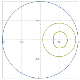
Figure 1. Subordinate Schur functions

In Figure 1, the outermost circle is the unit circle while the middle one is the image of $|z|=0.9$ under $f(z)$ which is again a circle with center at 1/2. The innermost figure is the image of $|z|=0.9$ under $f^{(1/2)}(z;1)$.

3.1. The change in Carathéodory function

Let the Carathéodory function associated with the perturbed Schur function $f^{(\beta_{k})}(z;k)$ be denoted by $\mathcal{C}^{(\beta_{k})}(z;k)$. Then, using (3.14), we can write

$$\mathcal{C}^{(\beta_{k})}(z;k) =\dfrac{1+zf^{(\beta_{k})}(z;k)}{1-zf^{(\beta_{k})}(z;k)}$$

$$=\dfrac{(\mathfrak{T}_{2,2}+z\mathfrak{T}_{1,2})+(\mathfrak{T}_{2,1}+z\mathfrak{T}_{1,1})f(z)}{(\mathfrak{T}_{2,2}-z\mathfrak{T}_{1,2})+(\mathfrak{T}_{2,1}-z\mathfrak{T}_{1,1})f(z)}.$$

Further, using the relation (1.19), we have

$$\mathcal{C}^{(\beta_{k})}(z;k)=\dfrac{\mathcal{Y}^{-}(z)+\mathcal{Y}^{+}(z)\mathcal{C}(z)}{\mathcal{W}^{-}(z)+\mathcal{W}^{+}(z)\mathcal{C}(z)},$$ (3.17)

where

$$\mathcal{Y}^{\pm}(z) =z(\mathfrak{T}_{(2,2)}+z\mathfrak{T}_{(1,2)})\pm(\mathfrak{T}_{(2,1)}+z\mathfrak{T}_{(1,1)})$$

$$\mathcal{W}^{\pm}(z) =z(\mathfrak{T}_{(2,2)}-z\mathfrak{T}_{(1,2)})\pm(\mathfrak{T}_{(2,1)}-z\mathfrak{T}_{(1,1)}).$$

As an illustration, for the Schur function $f(z)=(1+z)/2$, it is easy to verify that

$$\mathcal{C}(z)=\dfrac{2+z+z^{2}}{2-z-z^{2}}\quad\mbox{and}\quad\mathcal{C}^{(1/2)}(z;1)=\dfrac{2z^{3}-5z^{2}+7z+20}{-2z^{3}+7z^{2}-13z+20}.$$

We plot these Carathéodory functions below.

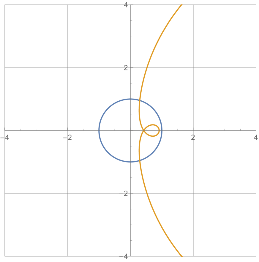
(a) The function $\mathcal{C}(z)$.

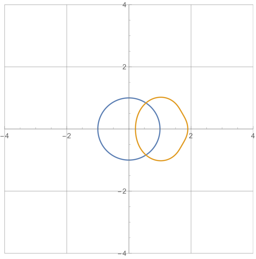
(b) The function $\mathcal{C}^{(1/2)}(z;1)$.

Figure 2. Perturbed mapping properties of Carathéodory functions.

In Figures 2(a) and 2(b), the ranges of both the original and perturbed Carathéodory functions are plotted for $|z|=0.9$. Interestingly, the range of $\mathcal{C}(z)$ is unbounded (Figure 2(a)) which is clear as $z=1$ is a pole of $\mathcal{C}(z)$. However $\mathcal{C}^{1/2}(z;1)$ has simple poles at 5/2 and $(1\pm i\sqrt{15})/2$ and hence with the use of perturbation we are able to make the range bounded (Figure 2(b)).

As shown in [23], the sequence $\{\gamma_{j}\}_{j=0}^{\infty}$ satisfying the recurrence relation

$$\gamma_{p+1}=\dfrac{\gamma_{p}-\bar{\alpha}_{p}}{1-\alpha_{p}\gamma_{p}},\quad p\geq 0.$$ (3.18)

where $\gamma_{0}=1$ and $\alpha_{j}^{\prime}s$ are the Schur parameters plays an important role in the $g$-fraction expansion for a special class of Carathéodory functions. Let $\{\gamma_{j}^{(\beta_{k})}\}$ correspond to the perturbed Carathéodory function $\mathcal{C}^{(\beta_{k})}(z;k)$. Since only $\alpha_{j}$ is perturbed, it is clear that $\gamma_{j}$ remains unchanged for $j=0,1,\cdots,k$. The first change, $\gamma_{k+1}$ to $\gamma_{k+1}^{(\beta_{k})}$, occurs when $\alpha_{k}$ is replaced by $\beta_{k}$. Consequently, $\gamma_{k+j}$, $j\geq 2$, change to $\gamma_{k+j}^{(\beta_{k})}$, $j\geq 2$, respectively. We now show that $\gamma_{j}$ can be expressed as a bilinear transformation of $\gamma_{j}^{(\beta_{k})}$ for $j\geq k+1$.

Theorem 3.2.

Let $\{\gamma_{j}\}_{j=0}^{\infty}$ be the sequence corresponding to $\{\alpha_{j}\}_{j=0}^{\infty}$ and $\{\gamma_{j}^{(\beta_{k})}\}_{j=0}^{\infty}$ that to $\{\alpha_{j}^{(\beta_{k})}\}_{j=0}^{\infty}$. Then,

$$\gamma_{k+j}^{(\beta_{k})}=\dfrac{\bar{a}_{k+j}\gamma_{k+j}-b_{k+j}}{-\bar{b}_{k+j}\gamma_{k+j}+a_{k+j}},\quad j\geq 1,$$ (3.19)

where

1. $a_{k+1}=\dfrac{1-\bar{\alpha}_{k}\beta_{k}}{1-|\beta_{k}|^{2}}\quad\mbox{and}\quad b_{k+1}=\dfrac{\bar{\beta_{k}}-\bar{\alpha}_{k}}{1-|\beta_{k}|^{2}}$, (j=1).

2. For $j\geq 2$,

   $$\left(\begin{array}[]{c}a_{k+j}\\ b_{k+j}\\ \end{array}\right)=\dfrac{1}{1-|\alpha_{k+j-1}|^{2}}\left(\begin{array}[]{cc}1&\alpha_{k+j-1}\\ \bar{\alpha}_{k+j-1}&1\\ \end{array}\right)\left(\begin{array}[]{cc}a_{k+j-1}-\bar{\alpha}_{k+j-1}\bar{b}_{k+j-1}\\ b_{k+j-1}-\bar{\alpha}_{k+j-1}\bar{a}_{k+j-1}\\ \end{array}\right).$$

Proof.

Consider first the expression

$$\dfrac{a_{k+1}\gamma_{k+1}^{(\beta_{k})}+b_{k+1}}{\bar{b}_{k+1}\gamma_{k+1}^{(\beta_{k})}+\bar{a}_{k+1}}.$$

Substituting $\gamma_{k+1}^{(\beta_{k})}=(\gamma_{k}-\bar{\beta}_{k})/(1-\beta_{k}\gamma_{k})$ and the given values of $a_{k+1}$ and $b_{k+1}$, it simplifies to

$$\dfrac{(1-\bar{\alpha}_{k}\beta_{k})(\gamma_{k}-\bar{\beta}_{k})+(\bar{\beta}_{k}-\bar{\alpha}_{k})(1-\alpha_{k}\gamma_{k})}{(\beta_{k}-\alpha_{k})(\gamma_{k}-\bar{\beta}_{k})+(1-\alpha_{k}\bar{\gamma}_{k})(1-\beta_{k}\gamma_{k})}=\dfrac{\gamma_{k}(1-|\beta_{k}|^{2})-\bar{\alpha}_{k}(1-|\beta_{k}|^{2})}{(1-|\beta_{k}|^{2})-\alpha_{k}\gamma_{k}(1-|\beta|^{2})}=\gamma_{k+1}.$$

Since $|a_{k+1}|^{2}-|b_{k+1}|^{2}=(1-|\alpha_{k}|^{2})/(1-|\beta_{k}|^{2})\neq 0$, (3.19) is proved for $j=1$.

Next, let

$$\dfrac{a_{k+2}\gamma_{k+2}^{(\beta_{k})}+b_{k+2}}{\bar{b}_{k+2}\gamma_{k+2}^{(\beta_{k})}+\bar{a}_{k+2}}=\dfrac{(a_{k+2}-\alpha_{k+1}b_{k+2})\gamma_{k+1}^{(\beta_{k})}+(b_{k+2}-\bar{\alpha}_{k+1}a_{k+2})}{(\bar{b}_{k+2}-\alpha_{k+1}\bar{a}_{k+2})\gamma_{k+1}^{(\beta_{k})}+(\bar{a}_{k+2}-\bar{\alpha}_{k+1}\bar{b}_{k+2})}=\dfrac{N(\gamma_{k})}{D(\gamma_{k})}.$$

Substituting first the given values of $a_{k+2}$ and $b_{k+2}$, the numerator becomes

$$N(\gamma_{k})=(1-|\alpha_{k+1}|^{2})[(a_{k+1}-\bar{\alpha}_{k+1}\bar{b}_{k+1})\gamma_{k+1}^{(\beta_{k})}+(b_{k+1}-\bar{\alpha}_{k+1}\bar{a}_{k+1})],$$

and then using, $\gamma_{k+1}^{(\beta_{k})}=(\bar{a}_{k+1}-b_{k+1})/(-\bar{b}_{k+1}\gamma_{k+1}+a_{k+1})$,

$$N(\gamma_{k})=(1-|\alpha_{k+1}|^{2})(|\alpha_{k+1}|^{2}-|b_{k+1}|^{2})(\gamma_{k+1}-\bar{\alpha}_{k+1}).$$

With similar calculations, we obtain

$$D(\gamma_{k})=(1-|\alpha_{k+1}|^{2})(|\alpha_{k+1}|^{2}-|b_{k+1}|^{2})(1-\alpha_{k+1}\gamma_{k+1}).$$

This means

$$\dfrac{N(\gamma_{k})}{D(\gamma_{k})}=\dfrac{\gamma_{k+1}-\bar{\alpha}_{k+1}}{1-\alpha_{k+1}\gamma_{k+1}}=\gamma_{k+2},$$

where $|a_{k+2}|^{2}-|b_{k+2}|^{2}=|a_{k+1}|^{2}-|b_{k+1}|^{2}\neq 0$, thus proving (3.19) for $j=2$. The remaining part of the proof is follows by a simple induction on $j$. ∎

Remark 3.1.

With the condition $|\alpha_{p}|<1$, it is clear that (3.18) gives analytic self-maps of the unit disk. Similar to the changes in mapping properties obtained as a consequence of perturbation, it is expected that (3.19) may lead to interesting results in fractal geometry and complex dynamics.

Remark 3.2.

Since $\gamma_{j}$ and $\gamma_{j}^{(\beta_{k})}$ are related by a bilinear transformation, it is clear that the expressions for $a_{k+j}$ and $b_{k+j}$, $j\geq 1$, are not unique.

It is known that if $\mathcal{C}(z)$ is real for real $z$, then the $\alpha_{p}^{\prime}s$ are real and $\gamma_{p}=1$, $p=0,1,\cdots$. Further, it is clear from (3.19) that $\gamma_{j}^{(\beta_{k})}=1$ whenever $\gamma_{j}=1$. In this case, the following $g$-fraction is obtained for $k\geq 0$.

$$\dfrac{1-z}{1+z}\mathcal{C}^{(\beta_{k})}(z)=\dfrac{1}{1}\begin{array}[]{cc}\\ $-$\end{array}\dfrac{g_{1}\omega}{1}\begin{array}[]{cc}\\ $-$\end{array}\dfrac{(1-g_{1})g_{2}\omega}{1}\begin{array}[]{cc}\\ $-$\end{array}\cdots\dfrac{(1-g_{k})g_{k+1}^{(\beta_{k})}\omega}{1}\begin{array}[]{cc}\\ $-$\end{array}\dfrac{(1-g_{k+1}^{(\beta_{k})})g_{k+2}\omega}{1}\begin{array}[]{cc}\\ $-$\end{array}\cdots$$

where $g_{j}=(1-\alpha_{j-1})/2$, $j=1,\cdots,k,k+2\cdots$, $g_{k+1}^{(\beta_{k})}=(1-\beta_{k})/2$ and $\omega=-4z/(1-z)^{2}$.

4. A class of Pick functions and Schur functions

Let the Hausdorff sequence $\{\nu_{j}\}_{j\geq 0}$ with $\nu_{0}=1$ be given so that there exists a bounded non-decreasing measure $\nu$ on [0,1] satisfying

$$\nu_{j}=\int_{0}^{1}\sigma^{j}d\nu(\sigma),\quad j\geq 0.$$

By [24, Theorem 69.2], the existence of $d\nu(\sigma)$ is equivalent to the power series

$$F(\omega)=\sum_{j\geq 0}\nu_{j}{\omega}^{j}=\int_{0}^{1}\dfrac{1}{1-\sigma\omega}d\nu(\sigma)$$

having a continued fraction expansion of the form

$$\int_{0}^{1}\dfrac{1}{1-\sigma\omega}d\nu(\sigma)=\dfrac{\nu_{0}}{1}\begin{array}[]{cc}\\ $-$\end{array}\dfrac{(1-g_{0})g_{1}\omega}{1}\begin{array}[]{cc}\\ $-$\end{array}\dfrac{(1-g_{1})g_{2}\omega}{1}\begin{array}[]{cc}\\ $-$\end{array}\dfrac{(1-g_{2})g_{3}\omega}{1}\begin{array}[]{cc}\\ $-$\end{array}\cdots$$

where $\nu_{0}\geq 0$ and $0\leq g_{p}\leq 1$, $p\geq 0$. Such functions $F(\omega)$ are analytic in the slit domain $\mathbb{C}\setminus[1,\infty)$ and belong to the class of Pick functions. We note that the Pick functions are analytic in the upper half plane and have a positive imaginary part [5].

In the next result, we characterize some members of the class of Pick functions using the gap $g$-fraction $\mathcal{F}_{2}^{(a,b,c)}(\omega)$. The proof is similar to that of [12, Theorem 1.5] and follows from [12, Lemma 3.1], given earlier as [15, Corollary 2.1].

Theorem 4.1.

If $a,b,c\in\mathbb{R}$ with $-1<a\leq c$ and $0\leq b\leq c$, then the functions

$$\omega \mapsto\dfrac{F(a+1,b+1;c+1;\omega)}{F(a+1,b;c+1;\omega)}\quad;\quad\omega\mapsto\dfrac{\omega F(a+1,b+1;c+1;\omega)}{F(a+1,b;c+1;\omega)}$$

$$\omega \mapsto\dfrac{F(a+2,b+1;c+2;\omega)}{F(a+1,b;c+1;\omega)}\quad;\quad\omega\mapsto\dfrac{zF(a+2,b+1;c+2;\omega)}{F(a+1,b;c+1;\omega)}$$

$$\omega \mapsto\dfrac{F(a+2,b+1;c+2;\omega)}{F(a+1,b+1;c+1;\omega)}\quad;\quad\omega\mapsto\dfrac{\omega F(a+2,b+1;c+2;\omega)}{F(a+1,b+1;c+1;\omega)}$$

are analytic in $\mathbb{C}\setminus[1,\infty)$ and each function map both the open unit disk $\mathbb{D}$ and the half plane $\{\omega\in\mathbb{C}:\mathrm{Re}\,\omega<1\}$ univalently onto domains that are convex in the direction of the imaginary axis.

We would like to note here that by a domain convex in the direction of imaginary axis, we mean that every line parallel to the imaginary axis has either connected or empty intersection with the corresponding domain [6], (see also [2, 12]. ).

Proof of Theorem 4.1.

With the given restrictions on $a$, $b$ and $c$, $\mathcal{F}_{2}^{(a,b,c)}(\omega)$ has a $g$-fraction expansion and hence by [24, Theorem 69.2], there exists a non-decreasing function $\nu_{0}:[0,1]\mapsto[0,1]$ with a total increase of 1 and

$$\dfrac{F(a+1,b+1;c+1;\omega)}{F(a+1,b;c+1;\omega)}=\int_{0}^{1}\dfrac{1}{1-\sigma\omega}d\nu_{0}(\sigma),\quad\omega\in\mathbb{C}\setminus[1,\infty),$$

which implies

$$\dfrac{\omega F(a+1,b+1;c+1;\omega)}{F(a+1,b;c+1;\omega)}=\int_{0}^{1}\dfrac{\omega}{1-\sigma\omega}d\nu_{0}(\sigma),\quad\omega\in\mathbb{C}\setminus[1,\infty).$$

Now, if we define

$$\nu_{1}(\sigma)=\dfrac{1}{k_{2}}\int_{0}^{\sigma}\rho d\nu_{0}(\rho),$$

where $k_{2}=(a+1)/(c+1)>0$, it can be easily seen that $\nu_{1}:[0,1]\mapsto[0,1]$ is again a non-decreasing map with $\nu_{1}(1)-\nu_{1}(0)=1$. Further, using the contiguous relation

$$F(a+1,b;c;\omega)-F(a,b;c;\omega)=\dfrac{b}{c}\omega F(a+1,b+1;c+1;\omega),$$ (4.1)

we obtain

$$\dfrac{\omega F(a+2,b+1;c+2;\omega)}{F(a+1,b;c+1;\omega)}=\int_{0}^{1}\dfrac{\omega}{1-\sigma\omega}d\nu_{1}(\sigma),\quad\omega\in\mathbb{C}\setminus[1,\infty),$$

and hence

$$\dfrac{F(a+1,b+1;c+1;\omega)}{F(a+1,b;c+1;\omega)}=1+k_{2}\int_{0}^{1}\dfrac{\omega}{1-\sigma\omega}d\nu_{1}(\sigma),\quad\omega\in\mathbb{C}\setminus[1,\infty).$$

Further, noting that the coefficient of $\omega$ in $F(a+2,b+1;c+2;\omega)/F(a+1,b;c+1;\omega)$ is $[(b+1)(c-a)]/[(c+1)(c+2)]=k_{3}+(1-k_{3})k_{2}$, we define

$$\nu_{2}(\sigma)=\dfrac{1}{k_{3}+k_{2}(1-k_{3})}\int_{0}^{\sigma}\rho d\nu_{1}(\rho),$$

and find that

$$\dfrac{F(a+2,b+1;c+2;\omega)}{F(a+1,b;c+1;\omega)}=1+[k_{3}+k_{2}(1-k_{3})]\int_{0}^{1}\dfrac{\omega}{1-\sigma\omega}d\nu_{2}(\sigma).$$

Finally from Gauss continued fraction (2.44), we conclude that $F(a+2,b+1;c+2;\omega)/F(a+1,b+1;c+1;\omega)$ has a $g$-fraction expansion and so there exists a map $\nu_{3}:[0,1]\mapsto[0,1]$ which is non-decreasing, $\nu_{3}(1)-\nu_{3}(0)=1$ and

$$\dfrac{\omega F(a+2,b+1;c+2;\omega)}{F(a+1;b+1;c+1;\omega)}=\int_{0}^{1}\dfrac{\omega}{1-\sigma\omega}d\nu_{3}(\sigma),\quad\omega\in\mathbb{C}\setminus[1,\infty).$$

Defining for $a<c$

$$\nu_{4}(\sigma)=\dfrac{1}{(1-k_{2})k_{3}}\int_{0}^{\sigma}\rho d\nu_{3}(\rho),$$

so that $(1-k_{2})k_{3}>0$, and using the fact that the coefficient of $\omega$ in $F(a+2,b+1;c+2;\omega)/F(a+1,b+1;c+1;\omega)$ is $(1-k_{2})k_{3}$, we obtain

$$\dfrac{F(a+2,b+1;c+2;\omega)}{F(a+1,b+1;c+1;\omega)}=1+[(1-k_{2})k_{3}]\int_{0}^{1}\dfrac{\omega}{1-\sigma\omega}d\nu_{4}(\sigma).$$

Thus, with $\nu_{j}$, $j=0,1,2,3,4$, satisfying the conditions of [12, Lemma 3.1], [15, Corollary 2.1], the proof of the theorem is completed. ∎

Remark 4.1.

Ratios of Gaussian hypergeometric functions having mapping properties described in Theorem 4.1 are also found in [12, Theorem 1.5] but for the ranges $-1\leq a\leq c$ and $0<b\leq c$. Hence for the common range $-1<a\leq c$ and $0<b\leq c$, two different ratios of hypergeometric functions belonging to the class of Pick functions can be obtained leading to the expectation of finding more such ratios for every possible range.

It may be noted that the ratio of Gaussian hypergeometric functions in (2.55) denoted here as $\mathcal{F}(z)$ has the mapping properties given in Theorem 4.1, which is proved in [12, Theorem 1.5]. We now consider its $g$-fraction expansion with the parameter $k_{2}$ missing. Using the contiguous relation (4.1) and the notations used in Theorems 2.1 and 2.4, it is clear that $\mathcal{F}_{3}^{(a,b,c)}(\omega)=F(a+2,b+1;c+2;\omega)/F(a+1,b+1;c+2;\omega)$ and

$$\mathcal{H}_{3}(\omega)=1-\dfrac{1}{\mathcal{F}_{3}^{(a,b,c)}(w)}=\dfrac{b+1}{c+2}\omega\dfrac{F(a+2,b+2;c+3;\omega)}{F(a+2,b+1;c+2;\omega)}.$$

Then

$$h(2;\omega)=(1-k_{1})\mathcal{H}_{3}(\omega)=\dfrac{(c-b)(b+1)}{(c)(c+2)}\omega\dfrac{F(a+2,b+2;c+3;\omega)}{F(a+2,b+1;c+2;\omega)}$$

Then, from Theorem 2.1,

$$\mathcal{F}(2;\omega) =\dfrac{1}{1-(1-k_{0})k_{1}\omega}-\dfrac{(1-k_{0})k_{1}\omega h(2;\omega)}{[1-(1-k_{0})k_{1}z]h(2;\omega)-[1-(1-k_{0})k_{1}z]^{2}}$$

$$=\dfrac{c}{c-bz}-\dfrac{bczh(2;z)}{c(c-bz)h(2;z)-(c-bz)^{2}}$$

which implies

$$\mathcal{F}(2;\omega)=\dfrac{c}{c-b\omega}-\dfrac{\dfrac{b(b+1)(c-b)}{c+2}\omega^{2}\dfrac{F(a+2,b+2;c+3;\omega)}{F(a+2,b+1;c+2;\omega)}}{\dfrac{(c-b)(b+1)(c-b\omega)}{c+2}\omega\dfrac{F(a+2,b+2;c+3;\omega)}{F(a+2,b+1;c+2;\omega)}-(c-b\omega)^{2}}$$

that is $\mathcal{F}(2;\omega)$ is given as a rational transformation of a new ratio of hypergeometric functions. It may also be noted that for $-1\leq a\leq c$ and $0<b\leq c$, [12, Theorem 1.5], both $\mathcal{F}(\omega)$ and $\mathcal{F}(2;\omega)$ will map both the unit disk $\mathbb{D}$ and the half plane $\{\omega\in\mathbb{C}:\mathrm{Re}\,\omega<1\}$ univalently onto domains that are convex in the direction of the imaginary axis.

As an illustration, we plot both these functions in figures (3(a)) and (3(b)).

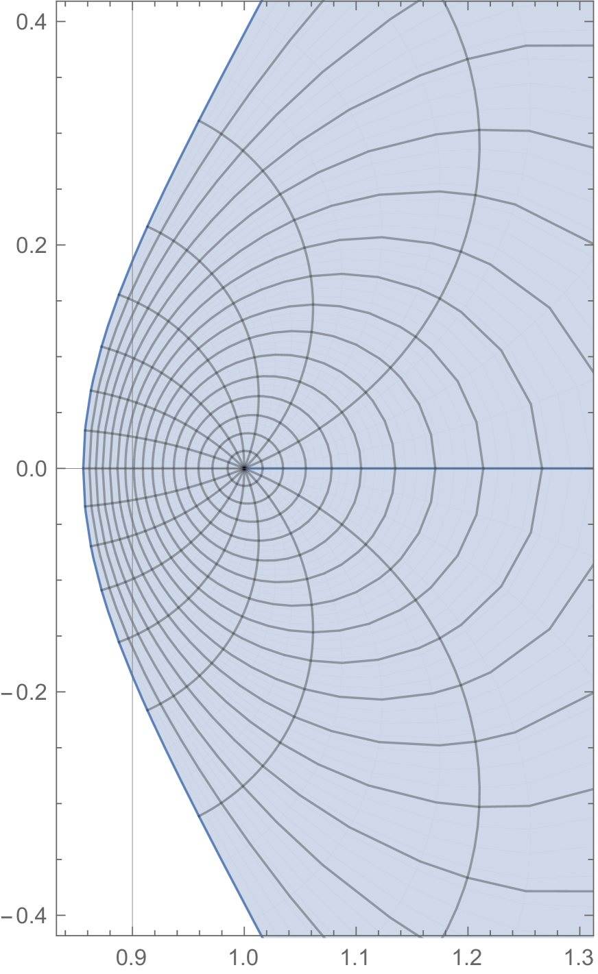
(a) The function $\mathcal{F}(\omega)$

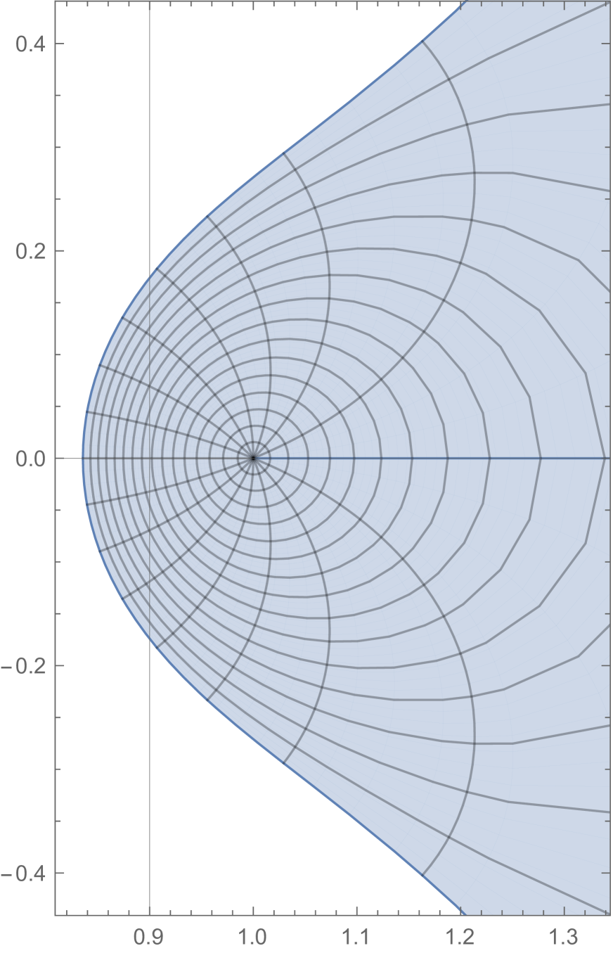
(b) The function $\mathcal{F}(2;\omega)$

Figure 3. The images of the disc $|\omega|<0.999$ under the mappings $\mathcal{F}(\omega)$ and $\mathcal{F}(2;z)$ for $a=0$, $b=0.1$, $c=0.4$.

4.1. A class of Schur functions

From Theorem 2.4 we obtain

$$\dfrac{k_{2j+1}\omega}{1-\dfrac{(1-k_{2j+1})k_{2j+2}\omega}{1-\dfrac{(1-k_{2j+2})k_{2j+3}\omega}{1-\cdots}}} =1-\dfrac{F(a+j,b+j;c+2j;\omega)}{F(a+j+1,b+j;c+2j;\omega)}$$

$$=\dfrac{b+j}{c+2j}\dfrac{\omega F(a+j+1,b+j+1;c+2j+1;\omega)}{F(a+j+1,b+j,c+2j;\omega)}$$

where the last equality follows from the contiguous relation (4.1) Hence using [23, eqns. 3.3 and 5.1] we get

$$\dfrac{1-z}{2}\dfrac{1-f_{2j}(z)}{1+zf_{2j}(z)}=\dfrac{b+j}{c+2j}\dfrac{F(a+j+1,b+j+1;c+2j+1;\omega)}{F(a+j+1,b+j,c+2j;\omega)},\quad j\geq 1,$$

where $f_{n}(z)$ is the Schur function and $\omega$ and $z$ are related as $\omega=-4z/(1-z)^{2}$. Similarly, interchanging $a$ and $b$ in (4.1) we obtain

$$\dfrac{1-z}{2}\dfrac{1-f_{2j+1}(z)}{1+zf_{2j+1}(z)}=\dfrac{a+j+1}{c+2j+1}\dfrac{F(a+j+2,b+j+1;c+2j+2;\omega)}{F(a+j+1,b+j+1,c+2j+1;\omega)},\quad j\geq 0,$$

where $\omega=-4z/(1-z)^{2}$.

Moreover, using the relation $\alpha_{j-1}=1-2k_{j}$, $j\geq 1$, the related sequence of Schur parameters is given by

$$\alpha_{j}=\left\{\begin{array}[]{ll}\dfrac{c-2b}{c+j},&\hbox{$j=2n$, $n\geq 0$;}\\ \dfrac{c-2a-1}{c+j},&\hbox{$j=2n+1$, $n\geq 1$.}\end{array}\right.$$

We note the following particular case. For $a=b-1/2$ and $c=b$, the resulting Schur parameters are $\alpha_{j}^{(b)}=-b/(b+j)$, $j\geq 0$. Such parameters have been considered in [19] (when $b\in\mathbb{R}$) in the context of orthogonal polynomials on the unit circle. These polynomials are known in modern literature as Szegö polynomials and we suggest the interested readers to refer [20] for further information.

Finally, as an illustration we note that while the Schur function associated with the parameters $\{\alpha_{j}^{(b)}\}_{j\geq 0}$ is $f(z)=-1$, that associated with the parameters $\{\alpha^{(b)}_{j}\}_{j\geq 1}$ is given by

$$\dfrac{1-z}{2}\dfrac{1-f^{(b)}(z)}{1+zf^{(b)}(z)}=\dfrac{b+1/2}{b+1}\dfrac{F(b+3/2,b+1;b+2;\omega)}{F(b+1/2,-;-;\omega)}$$

where $\omega=-4z/(1-z)^{2}$.

We remark that in this section, specific illustration of the results given in Section 2 are discussed leading to characterizing a class of ratio of hypergeometric functions. Similar characterization of functions involving the function $\omega=-4z/(1-z)^{2}$, given in Section 3 may provide some important consequences of such perturbation of $g$-fractions.

References

- [1] G. E. Andrews, R. Askey and R. Roy, Special functions, Encyclopedia of Mathematics and its Applications, 71, Cambridge Univ. Press, Cambridge, 1999.
- [2] Á. Baricz and A. Swaminathan, Mapping properties of basic hypergeometric functions, J. Class. Anal. 5 (2014), no. 2, 115–128.
- [3] K. Castillo, On perturbed Szegő recurrences, J. Math. Anal. Appl. 411 (2014), no. 2, 742–752.
- [4] K. Castillo, F. Marcellán and J. Rivero, On co-polynomials on the real line, J. Math. Anal. Appl. 427 (2015), no. 1, 469–483.
- [5] W. F. Donoghue, Jr., The interpolation of Pick functions, Rocky Mountain J. Math. 4 (1974), 169–173
- [6] P. L. Duren, Univalent functions, Grundlehren der Mathematischen Wissenschaften, 259, Springer-Verlag, New York(1983).
- [7] L. Garza and F. Marcellán, Szegő transformations and rational spectral transformations for associated polynomials, J. Comput. Appl. Math. 233 (2009), no. 3, 730–738.
- [8] M. E. H. Ismail, E. Merkes and D. Styer, A generalization of starlike functions, Complex Variables Theory Appl. 14 (1990), no. 1-4, 77-84.
- [9] W. B. Jones, O. Njåstad and W. J. Thron, Schur fractions, Perron Carathéodory fractions and Szegő polynomials, a survey, in Analytic theory of continued fractions, II (Pitlochry/Aviemore, 1985), 127–158, Lecture Notes in Math., 1199, Springer, Berlin.
- [10] W. B. Jones, O. Njåstad and W. J. Thron, Moment theory, orthogonal polynomials, quadrature, and continued fractions associated with the unit circle, Bull. London Math. Soc. 21 (1989), no. 2, 113–152.
- [11] W. B. Jones and W. J. Thron, Continued fractions, Encyclopedia of Mathematics and its Applications, 11, Addison-Wesley Publishing Co., Reading, MA, 1980.
- [12] R. Küstner, Mapping properties of hypergeometric functions and convolutions of starlike or convex functions of order , Comput. Methods Funct. Theory 2 (2002), no. 2, 597–610.
- [13] R. Küstner, On the order of starlikeness of the shifted Gauss hypergeometric function, J. Math. Anal. Appl. 334 (2007), no. 2, 1363–1385.
- [14] L. Lorentzen and H. Waadeland, Continued fractions with applications, Studies in Computational Mathematics, 3, North-Holland, Amsterdam, 1992.
- [15] E. P. Merkes, On typically-real functions in a cut plane, Proc. Amer. Math. Soc. 10 (1959), 863–868.
- [16] O. Njåstad, Convergence of the Schur algorithm, Proc. Amer. Math. Soc. 110 (1990), no. 4, 1003–1007.
- [17] J. Schur, Über Potenzreihen dei im Inneren des Einheitskreises beschränkt sind, J. reine angewandte Math. 147 (1917), 205–232, 148 (1918/19), 122–145.
- [18] B. Simon, Orthogonal polynomials on the unit circle. Part 1, American Mathematical Society Colloquium Publications, 54, Part 1, Amer. Math. Soc., Providence, RI, 2005.
- [19] A. Sri Ranga, Szegő polynomials from hypergeometric functions, Proc. Amer. Math. Soc. 138 (2010), no. 12, 4259–4270.
- [20] G. Szegő, Orthogonal polynomials, fourth edition, Amer. Math. Soc., Providence, RI, 1975.
- [21] A. V. Tsygvintsev, On the convergence of continued fractions at Runckel’s points, Ramanujan J. 15 (2008), no. 3, 407–413.
- [22] A. Tsygvintsev, Bounded analytic maps, Wall fractions and -flow, J. Approx. Theory 174 (2013), 206–219.
- [23] H. S. Wall, Continued fractions and bounded analytic functions, Bull. Amer. Math. Soc. 50 (1944), 110–119.
- [24] H. S. Wall, Analytic Theory of Continued Fractions, D. Van Nostrand Company, Inc., New York, NY, 1948.
- [25] A. Zhedanov, Rational spectral transformations and orthogonal polynomials, J. Comput. Appl. Math. 85 (1997), no. 1, 67–86.