Frequency conversion in ultrastrong cavity QED

Abstract

We propose a new method for frequency conversion of photons which is both versatile and deterministic. We show that a system with two resonators ultrastrongly coupled to a single qubit can be used to realize both single- and multiphoton frequency-conversion processes. The conversion can be exquisitely controlled by tuning the qubit frequency to bring the desired frequency-conversion transitions on or off resonance. Considering recent experimental advances in ultrastrong coupling for circuit QED and other systems, we believe that our scheme can be implemented using available technology.

I Introduction

Frequency conversion in quantum systems Kumar (1990); Huang and Kumar (1992) is important for many quantum technologies. The optimal working points of devices for transmission, detection, storage, and processing of quantum states are spread across a wide spectrum of frequencies O’Brien et al. (2009); Buluta et al. (2011). Interfacing the best of these devices is necessary to create quantum networks Kimble (2008) and other powerful combinations of quantum hardware. Examples of frequency-conversion setups developed for such purposes include upconversion for photon detection Albota and Wong (2004) and storage Tanzilli et al. (2005), since both these things are easier to achieve at a higher frequency than what is optimal for telecommunications. Downconversion in this frequency range has also been demonstrated Ou (2008); Ding and Ou (2010); Takesue (2010), and recently even strong coupling between a telecom and a visible optical mode Guo et al. (2016). Additionally, advances in quantum information processing with superconducting circuits at microwave frequencies You and Nori (2011); Devoret and Schoelkopf (2013) is driving progress on frequency conversion between optical and microwave frequencies Bochmann et al. (2013); Andrews et al. (2014); Shumeiko (2016); Hisatomi et al. (2016).

Circuit quantum electrodynamics (QED) You and Nori (2003); Wallraff et al. (2004); Blais et al. (2004); You and Nori (2011); Xiang et al. (2013) offers a wealth of possibilities for frequency conversion at microwave frequencies; some of these schemes can also be generalized to optical frequencies. By modulating the magnetic flux through a superconducting quantum interference device (SQUID) in a transmission line resonator, the frequency of the photons in the resonator can be changed rapidly Wallquist et al. (2006); Sandberg et al. (2008); Johansson et al. (2010) or two modes of the resonator can be coupled Chirolli et al. (2010); Zakka-Bajjani et al. (2011). Other driven Josephson-junction-based devices can also be used for microwave frequency conversion Abdo et al. (2013); Kamal et al. (2014). Downconversion has been proposed for setups with $\Delta$-type three-level atoms Marquardt (2007); Koshino (2009); Sánchez-Burillo et al. (2016) and demonstrated with an effective three-level $\Lambda$ system Inomata et al. (2014). Upconversion of a two-photon drive has been shown for a flux qubit coupled to a resonator in a way that breaks parity symmetry Deppe et al. (2008). Indeed, the $\Delta$-type level structure in a flux qutrit Liu et al. (2005) even makes possible general three-wave mixing Liu et al. (2014). Recently, frequency conversion was also demonstrated for two sideband-driven microwave $LC$-resonators coupled through a mechanical resonator Lecocq et al. (2016).

The approach to frequency conversion that we propose in this article is based on two cavities or resonator modes coupled ultrastrongly to a two-level atom (qubit). The regime of ultrastrong coupling (USC), where the coupling strength starts to become comparable to the bare transition frequencies in the system, has only recently been reached in a number of solid-state systems Günter et al. (2009); Forn-Díaz et al. (2010); Niemczyk et al. (2010); Todorov et al. (2010); Schwartz et al. (2011); Scalari et al. (2012); Geiser et al. (2012); Kéna-Cohen et al. (2013); Gambino et al. (2014); Maissen et al. (2014); Goryachev et al. (2014); Baust et al. (2016); Forn-Díaz et al. (2017); Yoshihara et al. (2017); Chen et al. (2016); George et al. (2016); Langford et al. (2016); Braumüller et al. (2016); Yoshihara et al. (2016). Among these, a few circuit-QED experiments provide some of the clearest examples Forn-Díaz et al. (2010); Niemczyk et al. (2010); Baust et al. (2016); Forn-Díaz et al. (2017); Yoshihara et al. (2017); Chen et al. (2016); Langford et al. (2016); Braumüller et al. (2016); Yoshihara et al. (2016), including the largest coupling strength reported Yoshihara et al. (2017). While the USC regime displays many striking physical phenomena De Liberato et al. (2007); Ashhab and Nori (2010); Cao et al. (2010, 2011); Stassi et al. (2013); Sanchez-Burillo et al. (2014); De Liberato (2014); Lolli et al. (2015); Di Stefano et al. (2016); Cirio et al. (2016), we are here only concerned with the fact that it enables higher-order processes that do not conserve the number of excitations in the system, an effect which has also been noted for a multilevel atom coupled to a resonator Zhu et al. (2013). Examples of such processes include multiphoton Rabi oscillations Ma and Law (2015); Garziano et al. (2015) and a single photon exciting multiple atoms Garziano et al. (2016). Indeed, almost any analogue of processes from nonlinear optics is feasible Kockum et al. (2017); this can be regarded as an example of quantum simulation Buluta and Nori (2009); Georgescu et al. (2014). Just like the analytical solution for the quantum Rabi model Braak (2011) is now being extended to multiple qubits Braak (2013); Peng et al. (2013) and multiple resonators Chilingaryan and Rodríguez-Lara (2015); Duan et al. (2015); Alderete and Rodríguez-Lara (2016), we here extend the exploration of non-excitation-conserving processes to multiple resonators.

In our proposal, the qubit frequency is tuned to make various frequency-converting transitions resonant. For example, making the energy of a single photon in the first resonator equal to the sum of the qubit energy and the energy of a photon in the second resonator enables the conversion of the former (a high-energy photon) into the latter (a low-energy photon plus a qubit excitation) and vice versa. In the same way, a single photon in the first resonator can be converted into multiple photons in the second resonator (and vice versa) if the qubit energy is tuned to make such a transition resonant. The proposed frequency-conversion scheme is deterministic and allows for a variety of different frequency-conversion processes in the same setup. The setup should be possible to implement in state-of-the-art circuit QED, but the idea also applies to other cavity QED systems.

We note that the process of parametric down-conversion in this type of circuit-QED setup has been considered previously Moon and Girvin (2005), but in a regime of weaker coupling and without using the qubit to control the process. Also, it has been shown that a beamsplitter-type coupling between two resonators can be controlled by changing the qubit state Mariantoni et al. (2008) or induced for weaker qubit-resonator coupling by driving the qubit Prado et al. (2006), but the proposal presented here offers greater versatility and simplicity for frequency conversion.

This article is organized as follows. In Sec. II, we define the system under consideration and explain the principle behind frequency conversion based on USC. In Secs. III and IV, we show the details of the single- and multiphoton frequency-conversion processes, respectively, including both analytical and numerical calculations. We conclude and give an outlook for future work in Sec. V. Details of some analytical calculations are given in Appendix A.

II Model

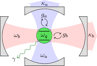
Figure 1: A sketch of the system. A qubit (green) is coupled to two resonator modes (blue, $a$, and red, $b$). Decoherence channels for the qubit (relaxation rate $\gamma$) and the resonators (relaxation rates $\kappa_{a}$, $\kappa_{b}$) are included.

We consider a setup where a qubit with transition frequency $\omega_{q}$ is coupled to two resonators with resonance frequencies $\omega_{a}$ and $\omega_{b}$, respectively, as sketched in Fig. 1. The Hamiltonian is ($\hbar=1$)

$$\hat{H} = \omega_{a}\hat{a}^{\dagger}\hat{a}+\omega_{b}\hat{b}^{\dagger}\hat{b}+\frac{\omega_{q}}{2}\hat{\sigma}_{z}$$ (1)

$$+\left[g_{a}\left(\hat{a}+\hat{a}^{\dagger}\right)+g_{b}\left(\hat{b}+\hat{b}^{\dagger}\right)\right]$$

$$\times\left(\hat{\sigma}_{x}\cos\theta+\hat{\sigma}_{z}\sin\theta\right),$$

where $g_{a}$ ($g_{b}$) denotes the strength of the coupling between the qubit and the first (second) resonator. The creation and annihilation operators for photons in the first (second) resonator are $\hat{a}$ and $\hat{a}^{\dagger}$ ($\hat{b}$ and $\hat{b}^{\dagger}$), respectively. The angle $\theta$ parameterizes the amount of longitudinal and transverse coupling as, for example, in experiments with flux qubits You et al. (2007); Deppe et al. (2008); Niemczyk et al. (2010); Forn-Díaz et al. (2010); Baust et al. (2016); Yoshihara et al. (2016); $\hat{\sigma}_{x}$ and $\hat{\sigma}_{z}$ are Pauli matrices for the qubit.

Note that we do not include a direct coupling between the two resonators. Such a coupling is seen in experiments Baust et al. (2016), but here we will only be concerned with situations where the resonators are far detuned from each other, meaning that this coupling term can safely be neglected. Likewise, we do not include higher modes of the resonators. While they may contribute in experiments with cavities and transmission-line resonators, they can be avoided by using lumped-element resonators Kim et al. (2011); Yoshihara et al. (2016).

The crucial feature of Eq. (1) for our frequency-conversion scheme is that some of the coupling terms do not conserve the number of excitations in the system. The $\hat{\sigma}_{z}$ coupling terms act to change the photon number in one of the resonators by one, while keeping the number of qubit excitations unchanged. Likewise, the $\hat{\sigma}_{x}$ coupling contains terms like $\hat{a}\hat{\sigma}_{-}$ and $\hat{b}^{\dagger}\hat{\sigma}_{+}$ that change the number of excitations in the system by two. For weak coupling strengths, all such terms can be neglected using the rotating-wave approximation (RWA), but in the USC regime the higher-order processes that these terms enable can become important and function as second- or third-order nonlinearities in nonlinear optics Kockum et al. (2017).

To include the effect of decoherence in our system, we use a master equation on the Lindblad form in our numerical simulations. The master equation reads

$$\dot{\hat{\rho}}=-i\left[\hat{H},\hat{\rho}\right]+\sum_{j,k>j}\left(\Gamma_{a}^{jk}+\Gamma_{b}^{jk}+\Gamma_{q}^{jk}\right)\mathcal{D}\left[\left|j\rangle\langle k\right|\right]\hat{\rho},$$ (2)

where $\hat{\rho}$ is the density matrix of the system, $\mathcal{D}\left[\hat{c}\right]\rho=\hat{c}\hat{\rho}\hat{c}^{\dagger}-\frac{1}{2}\hat{\rho}\hat{c}^{\dagger}\hat{c}-\frac{1}{2}\hat{c}^{\dagger}\hat{c}\hat{\rho}$, and the states in the sum are eigenstates of the USC system. The relaxation rates are given by $\Gamma_{a}^{jk}=\kappa_{a}\left|X_{a}^{jk}\right|^{2}$, $\Gamma_{b}^{jk}=\kappa_{b}\left|X_{b}^{jk}\right|^{2}$, and $\Gamma_{q}^{jk}=\gamma\left|C^{jk}\right|^{2}$, where $c^{jk}=\left\langle j\left|\hat{c}\right|k\right\rangle$ with $\hat{X}_{a}=\hat{a}+\hat{a}^{\dagger}$, $\hat{X}_{b}=\hat{b}+\hat{b}^{\dagger}$, and $\hat{C}=\hat{\sigma}_{x}$ Beaudoin et al. (2011); Ridolfo et al. (2012). Writing the master equation in the eigenbasis of the full system avoids unphysical effects, such as emission of photons from the ground state. Similarly, to correctly count the number of photonic and qubit excitations we use $\left\langle\hat{X}_{a}^{-}\hat{X}_{a}^{+}\right\rangle$, $\left\langle\hat{X}_{b}^{-}\hat{X}_{b}^{+}\right\rangle$, and $\left\langle\hat{C}^{-}\hat{C}^{+}\right\rangle$, where the plus and minus signs denote the positive and negative frequency parts, respectively, of the operators in the system eigenbasis, instead of $\left\langle\hat{a}^{\dagger}\hat{a}\right\rangle$, $\left\langle\hat{b}^{\dagger}\hat{b}\right\rangle$, and $\left\langle\hat{\sigma}_{+}\hat{\sigma}_{-}\right\rangle$ Ridolfo et al. (2012).

III Single-photon frequency conversion

We first consider single-photon frequency conversion, where one photon in the first resonator is converted into one photon of a different frequency in the second resonator, or vice versa. The conversion is aided by the qubit. Without loss of generality, we take $\omega_{a}>\omega_{b}$. For the conversion to work, we then need $\omega_{a}\approx\omega_{b}+\omega_{q}$, such that the states $|1,0,g\rangle$ and $|0,1,e\rangle$ are close to resonant. Due to the presence of longitudinal coupling in the Hamiltonian in Eq. (1), transitions between these two states are possible even though their excitation numbers and parity differ.

Figure 2: The four lowest-order processes contributing to a transition between $|1,0,g\rangle$ and $|0,1,e\rangle$. For this illustration, the parameter values $\omega_{a}=3\omega_{q}$ and $\omega_{b}=2\omega_{q}$ were used to set the positions of the energy levels. The transitions that do not conserve excitation number are shown as dashed lines, and the excitation-number-conserving transitions are shown as solid lines. Red lines correspond to $\hat{\sigma}_{z}$ (longitudinal) coupling and blue lines to $\hat{\sigma}_{x}$ (transverse) coupling in the Hamiltonian given in Eq. (1). Each transition is labelled by its matrix element.

The intermediate states and transitions contributing (in lowest order) to the $|1,0,g\rangle\leftrightarrow|0,1,e\rangle$ transition are shown in Fig. 2. Virtual transitions to and from one of the four intermediate states $|0,0,g\rangle$, $|0,0,e\rangle$, $|1,1,g\rangle$, and $|1,1,e\rangle$ connect $|1,0,g\rangle$ and $|0,1,e\rangle$ in two steps. This is the minimum number of steps possible, since the terms in the Hamiltonian in Eq. (1) can only create or annihilate a single photon at a time. From the figure, it is also clear that no path exists between $|1,0,g\rangle$ and $|0,1,e\rangle$ that does not involve longitudinal coupling (dashed red arrows in the figure).

To calculate the effective coupling between the states $|1,0,g\rangle$ and $|0,1,e\rangle$, we truncate the Hamiltonian from Eq. (1) to the six states shown in Fig. 2. Written on matrix form, this truncated Hamiltonian becomes

$$\hat{H}=\begin{pmatrix}-\frac{\omega_{q}}{2}&0&-g_{a}\sin\theta&g_{b}\cos\theta&0&0\\ 0&\frac{\omega_{q}}{2}&g_{a}\cos\theta&g_{b}\sin\theta&0&0\\ -g_{a}\sin\theta&g_{a}\cos\theta&\omega_{a}-\frac{\omega_{q}}{2}&0&-g_{b}\sin\theta&g_{b}\cos\theta\\ g_{b}\cos\theta&g_{b}\sin\theta&0&\omega_{b}+\frac{\omega_{q}}{2}&g_{a}\cos\theta&g_{a}\sin\theta\\ 0&0&-g_{b}\sin\theta&g_{a}\cos\theta&\omega_{a}+\omega_{b}-\frac{\omega_{q}}{2}&0\\ 0&0&g_{b}\cos\theta&g_{a}\sin\theta&0&\omega_{a}+\omega_{b}+\frac{\omega_{q}}{2}\end{pmatrix},$$ (3)

where the states are ordered from left to right as $|0,0,g\rangle$, $|0,0,e\rangle$, $|1,0,g\rangle$, $|0,1,e\rangle$, $|1,1,g\rangle$, and $|1,1,e\rangle$. When the condition $\omega_{a}\approx\omega_{b}+\omega_{q}$ is satisfied, the four intermediate states $|0,0,g\rangle$, $|0,0,e\rangle$, $|1,1,g\rangle$, and $|1,1,e\rangle$ can be adiabatically eliminated. This calculation, shown in Appendix A.1, gives an effective Hamiltonian with a coupling term

$$\hat{H}_{\rm c,eff}=g_{\rm eff}\left(\left|1,0,g\rangle\langle 0,1,e\right|+\left|0,1,e\rangle\langle 1,0,g\right|\right),$$ (4)

where the effective coupling between the states $|1,0,g\rangle$ and $|0,1,e\rangle$ has the magnitude

$$g_{\rm eff}=g_{a}g_{b}\sin 2\theta\left(\frac{1}{\omega_{b}}-\frac{1}{\omega_{a}}\right)$$ (5)

on resonance. Compared to the direct resonator-qubit coupling in Eq. (1), $g_{\rm eff}$ is weaker by a factor of order $g/\omega$, which is why we need to at least approach the USC regime to observe the single-photon frequency conversion. We note that the effective coupling is maximized when the longitudinal and transverse coupling terms in Eq. (1) have equal magnitude. Interestingly, Eq. (5) suggests that frequency conversion can be more efficient if $\omega_{b}\ll\omega_{a}$. However, going too far in this direction violates the assumptions behind the adiabatic approximation, which relies on $g_{a},g_{b}\ll\omega_{a},\omega_{b}$.

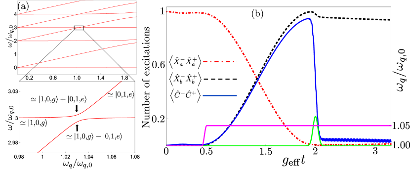
Figure 3: Two frequency conversion methods. (a) The figure shows the energy levels of our system plotted as a function of the qubit frequency $\omega_{q}$, using the parameters $g_{a}=g_{b}=0.15\omega_{q,0}$, $\theta=\pi/6$, $\omega_{a}=3\omega_{q,0}$, and $\omega_{b}=2\omega_{q,0}$, where $\omega_{q,0}$ is a reference point for the qubit frequency, set such that $\omega_{a}=\omega_{b}+\omega_{q,0}$. In the zoom-in, close to the resonance $\omega_{a}=\omega_{b}+\omega_{q}$, we see the anticrossing between $|1,0,g\rangle$ and $|0,1,e\rangle$ with splitting $2g_{\rm eff}$. Up- or down-conversion of single photons can be achieved by adiabatically tuning $\omega_{q}$ to follow one of the energy levels in the figure from $|1,0,g\rangle$ to $|0,1,e\rangle$, or vice versa. (b) A rapid frequency conversion can be achieved by starting in $|1,0,g\rangle$, far from the resonance $\omega_{a}=\omega_{b}+\omega_{q}$, tuning the qubit frequency (pink solid line) into resonance for half a Rabi period ($\pi/2g_{\rm eff}$) and then sending a pulse (green solid line) to deexcite the qubit. The figure shows the number of excitations in the two resonators (red dashed-dotted line for $a$, black dashed line for $b$) and the qubit (blue solid line) during such a process, including decoherence in the form of relaxation from the resonators and the qubit. The parameters used for the decoherence are $\kappa_{a}=\kappa_{b}=\gamma=4\times 10^{-5}\omega_{q,0}$.

The existence of this effective coupling suggests at least two ways to perform single-photon frequency conversion. The first is to use adiabatic transfer, starting in $|1,0,g\rangle$ ($|0,1,e\rangle$) with the qubit frequency sufficiently far detuned from the resonance $\omega_{a}=\omega_{b}+\omega_{q}$ and then slowly (adiabatically) changing the qubit frequency until the system ends up in the state $|0,1,e\rangle$ ($|1,0,g\rangle$), following one of the energy levels shown in Fig. 3(a). In this way, a single photon in the first (second) resonator is deterministically down-converted (up-converted) to a single photon of lower (higher) frequency in the second (first) resonator. We note that such adiabatic transfer has been used for robust single-photon generation in circuit QED, tuning the frequency of a transmon qubit to achieve the transition $|0,e\rangle\to|1,g\rangle$ Johnson et al. (2010). It has also been suggested as a method to generate multiple photons from a single qubit excitation in the USC regime of the standard quantum Rabi model Ma and Law (2015).

The second approach, exemplified by a simulation including decoherence in Fig. 3(b), is to initialize the system in one of the states $|1,0,g\rangle$ or $|0,1,e\rangle$, far from the frequency-conversion resonance such that the effective coupling is negligible, quickly tune the qubit into resonance for the duration of half a Rabi oscillation period (set by the effective coupling to be $\pi/2g_{\rm eff}$), and then detune the qubit again (or send a pulse to deexcite it) to turn off the effective interaction. This type of scheme is, for example, commonly used for state transfer between resonators and/or qubits in circuit QED Sillanpää et al. (2007); Hofheinz et al. (2008, 2009); Wang et al. (2011); Mariantoni et al. (2011). Letting the resonance last shorter or longer times, any superposition of $|1,0,g\rangle$ or $|0,1,e\rangle$ can be created. The potential for creating superpositions of photons of different frequencies (similar to Ref. Zakka-Bajjani et al. (2011)) with such a method will be explored in future work.

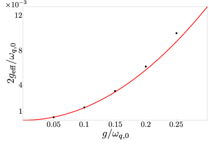
Figure 4: Comparison of analytical (red line) and numerical (black dots) results for the effective coupling between the states $|1,0,g\rangle$ and $|0,1,e\rangle$. The graph shows the minimum energy splitting $2g_{\rm eff}/\omega_{q,0}$ as a function of $g/\omega_{q,0}$, where $g=g_{a}=g_{b}$, using the same parameters as in Fig. 3.

Since the relevant timescales for both these approaches are determined by $g_{\rm eff}$, it is important to know in which parameter range the expression for $g_{\rm eff}$ given in Eq. (5) remains a good approximation. In Fig. 4, we show that the expression is valid up to at least $g_{a}=g_{b}=0.2\omega_{q,0}$ for the parameters used in Fig. 3.

IV Multi-photon frequency conversion

We now turn to multi-photon frequency conversion, where, aided by the qubit, one photon in the first resonator is converted into two photons in the second resonator, or vice versa. We continue to adopt the convention that $\omega_{a}>\omega_{b}$. In contrast to the single-photon frequency conversion case in Sec. III, there are now two possibilities for how the qubit state can change during the conversion process. Below, we will study both $|1,0,g\rangle\leftrightarrow|0,2,e\rangle$ and $|1,0,e\rangle\leftrightarrow|0,2,g\rangle$. Since we wish to use the qubit to control the process, we do not consider the process $|1,0,g\rangle\leftrightarrow|0,2,g\rangle$, which to some extent was already included in Ref. Moon and Girvin (2005).

IV.1 $|1,0,g\rangle\leftrightarrow|0,2,e\rangle$

For the process $|1,0,g\rangle\leftrightarrow|0,2,e\rangle$, we first of all note one more difference compared to the single-photon frequency conversion case in Sec. III: it changes the number of excitations from 1 to 3, which means that excitation-number parity is conserved. This makes the longitudinal coupling of Eq. (1) redundant for achieving the conversion, and to simplify our calculations we therefore hereafter work with the standard quantum Rabi Hamiltonian Rabi (1937) extended to two resonators,

$$\hat{H}_{\rm R} = \omega_{a}\hat{a}^{\dagger}\hat{a}+\omega_{b}\hat{b}^{\dagger}\hat{b}+\frac{\omega_{q}}{2}\hat{\sigma}_{z}$$ (6)

$$+\left[g_{a}\left(\hat{a}+\hat{a}^{\dagger}\right)+g_{b}\left(\hat{b}+\hat{b}^{\dagger}\right)\right]\hat{\sigma}_{x}.$$

Figure 5: The lowest-order processes contributing to a transition between $|1,0,g\rangle$ and $|0,2,e\rangle$ in the quantum Rabi model. The transitions that do not conserve excitation number are shown as dashed blue lines and the excitation-number-conserving transitions are shown as solid blue lines. The label of each line is the term in Eq. (6) that gives rise to that transition. The parameters $\omega_{a}=5\omega_{q}$ and $\omega_{b}=2\omega_{q}$ were used to set the positions of the energy levels.

Placing the system close to the resonance $\omega_{a}=2\omega_{b}+\omega_{q}$, virtual transitions involving the intermediate states $|0,0,e\rangle$, $|0,1,g\rangle$, $|1,1,e\rangle$, and $|1,2,g\rangle$ (to lowest order), contribute to the process $|1,0,g\rangle\leftrightarrow|0,2,e\rangle$, as shown in Fig. 5. The most direct path between $|1,0,g\rangle$ and $|0,2,e\rangle$ involves three steps, since only one photon can be created or annihilated in each step. We note that all the paths include at least one transition that is due to terms in the Hamiltonian that do not conserve excitation number (dashed arrows in the figure).

Retaining only the states shown in Fig. 5, we can write the quantum Rabi Hamiltonian from Eq. (6) on matrix form as

$$\hat{H}_{\rm R}=\begin{pmatrix}\frac{\omega_{q}}{2}&g_{b}&g_{a}&0&0&0\\ g_{b}&\omega_{b}-\frac{\omega_{q}}{2}&0&\sqrt{2}g_{b}&g_{a}&0\\ g_{a}&0&\omega_{a}-\frac{\omega_{q}}{2}&0&g_{b}&0\\ 0&\sqrt{2}g_{b}&0&2\omega_{b}+\frac{\omega_{q}}{2}&0&g_{a}\\ 0&g_{a}&g_{b}&0&\omega_{a}+\omega_{b}+\frac{\omega_{q}}{2}&\sqrt{2}g_{b}\\ 0&0&0&g_{a}&\sqrt{2}g_{b}&\omega_{a}+2\omega_{b}-\frac{\omega_{q}}{2}\end{pmatrix},$$ (7)

where the states are ordered as $|0,0,e\rangle$, $|0,1,g\rangle$, $|1,0,g\rangle$, $|0,2,e\rangle$, $|1,1,e\rangle$, and $|1,2,g\rangle$. Just like in Sec. III, we can adiabatically eliminate the intermediate states when the condition $\omega_{a}\approx 2\omega_{b}+\omega_{q}$ is satisfied. The result of this calculation, the details of which are given in Appendix A.2, is an effective coupling between the states $|1,0,g\rangle$ and $|0,2,e\rangle$ with magnitude

$$g_{\rm eff}=\frac{\sqrt{2}g^{3}\left[2\omega_{b}(\omega_{a}-2\omega_{b})-g^{2}\right]}{2\omega_{b}^{2}(\omega_{a}-\omega_{b})^{2}+g^{2}\omega_{b}(5\omega_{b}-3\omega_{a})+g^{4}}$$ (8)

on resonance. Here, we have set $g_{a}=g_{b}\equiv g$ to simplify the expression slightly. We note that, to leading order, the coupling scales like $g^{3}/\omega^{2}$; indeed, the leading-order term is

$$g_{\rm eff}=\frac{\sqrt{2}g^{3}\left(\omega_{a}-2\omega_{b}\right)}{\omega_{b}\left(\omega_{a}-\omega_{b}\right)^{2}}.$$ (9)

This is a factor $g/\omega$ weaker than for the single-photon frequency conversion, and reflects the fact that an additional intermediate transition is required for the two-photon conversion. We also note that the coupling becomes small in the limit of small $\omega_{q}$, i.e., when $2\omega_{b}\to\omega_{a}$. The coupling would become large if $\omega_{a}\to\omega_{b}$, but this is impossible since $\omega_{a}=2\omega_{b}+\omega_{q}$ in this scheme.

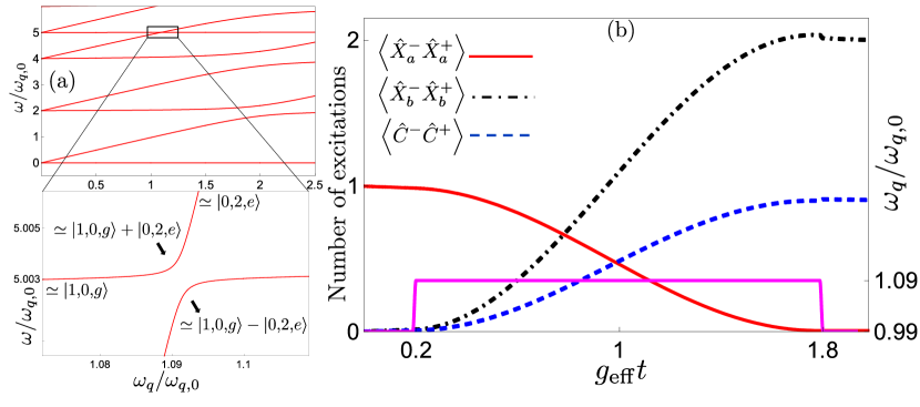
Figure 6: Two-photon frequency conversion via transitions between $|1,0,g\rangle$ and $|0,2,e\rangle$. (a) The energy levels of our system, given in Eq. (6), plotted as a function of the qubit frequency $\omega_{q}$, using the parameters $g_{a}=g_{b}=0.2\omega_{q,0}$, $\omega_{a}=5\omega_{q,0}$, and $\omega_{b}=2\omega_{q,0}$, where the reference point $\omega_{q,0}$ is set such that $\omega_{a}=2\omega_{b}+\omega_{q,0}$. In the zoom-in, close to the resonance $\omega_{a}=2\omega_{b}+\omega_{q}$, we see the anticrossing between $|1,0,g\rangle$ and $|0,2,e\rangle$ with the splitting $2g_{\rm eff}$ given by Eq. (8). Up-conversion of a photon pair into a single photon, or down-conversion of a single photon into a photon pair, can be achieved by adiabatically tuning $\omega_{q}$ to follow one of the energy levels in the figure from $|0,2,e\rangle$ to $|1,0,g\rangle$, or vice versa. (b) A rapid frequency conversion can be achieved by starting in $|1,0,g\rangle$ or $|0,2,e\rangle$, far from the resonance $\omega_{a}=2\omega_{b}+\omega_{q}$, tuning the qubit frequency (pink solid line) into resonance for half a Rabi period ($\pi/2g_{\rm eff}$) and then tuning it out of resonance again. The figure shows the number of excitations in the two resonators (red solid line for $a$, black dashed-dotted line for $b$) and the qubit (blue dashed line) during such a process, including decoherence in the form of relaxation from the resonators and the qubit. The parameters used for the decoherence are $\kappa_{a}=\kappa_{b}=\gamma=2\times 10^{-5}\omega_{q,0}$.

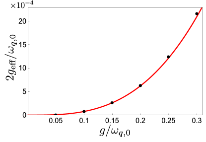
Figure 7: Comparison of analytical (red line) and numerical (black dots) results for the effective coupling between the states $|1,0,g\rangle$ and $|0,2,e\rangle$. The graph shows the minimum energy splitting $2g_{\rm eff}/\omega_{q,0}$ as a function of $g/\omega_{q,0}$, using the same parameters as in Fig. 6.

The two-photon frequency conversion can be performed either by adiabatic transfer or by tuning the qubit into resonance for half a Rabi oscillation period, as explained in Sec. III. In the first approach, one adiabatically tunes the qubit energy to follow one of the energy levels shown in Fig. 6(a). A simulation of the second approach, including decoherence, is shown in Fig. 6(b). The timescale for these processes is set by the effective coupling. In Fig. 7, we show that the expression for the effective coupling given in Eq. (8) remains a good approximation up to at least $g=0.3\omega_{q,0}$ for the parameters used in Fig. 6.

IV.2 $|1,0,e\rangle\leftrightarrow|0,2,g\rangle$

Figure 8: The lowest-order processes contributing to a transition between $|1,0,e\rangle$ and $|0,2,g\rangle$ in the quantum Rabi model. The transitions that do not conserve excitation number are shown as dashed blue lines and the excitation-number-conserving transitions are shown as solid blue lines. The label of each line is the term in Eq. (6) that gives rise to that transition. The parameters $\omega_{a}=3\omega_{q}$ and $\omega_{b}=2\omega_{q}$ were used to set the positions of the energy levels.

For the process $|1,0,e\rangle\leftrightarrow|0,2,g\rangle$, we show in Fig. 8 the virtual transitions from the quantum Rabi Hamiltonian that contribute to lowest order. We note that this process conserves the excitation number, which means that there is a path between the states that can be realized using only terms from the Jaynes–Cummings (JC) Hamiltonian Jaynes and Cummings (1963) (solid arrows in the figure). Below, we analyze the effective coupling both for the full quantum Rabi Hamiltonian and for the JC Hamiltonian.

IV.2.1 Quantum Rabi Hamiltonian

Retaining only the states shown in Fig. 8, we can write the quantum Rabi Hamiltonian from Eq. (6) on matrix form as

$$\hat{H}_{\rm R}=\begin{pmatrix}-\frac{\omega_{q}}{2}&g_{b}&g_{a}&0&0&0\\ g_{b}&\omega_{b}+\frac{\omega_{q}}{2}&0&\sqrt{2}g_{b}&g_{a}&0\\ g_{a}&0&\omega_{a}+\frac{\omega_{q}}{2}&0&g_{b}&0\\ 0&\sqrt{2}g_{b}&0&2\omega_{b}-\frac{\omega_{q}}{2}&0&g_{a}\\ 0&g_{a}&g_{b}&0&\omega_{a}+\omega_{b}-\frac{\omega_{q}}{2}&\sqrt{2}g_{b}\\ 0&0&0&g_{a}&\sqrt{2}g_{b}&\omega_{a}+2\omega_{b}+\frac{\omega_{q}}{2}\end{pmatrix},$$ (10)

where the states are ordered as $|0,0,g\rangle$, $|0,1,e\rangle$, $|1,0,e\rangle$, $|0,2,g\rangle$, $|1,1,g\rangle$, and $|1,2,e\rangle$. As in previous calculations, we can perform adiabatic elimination close to the resonance, which in this case is $\omega_{a}+\omega_{q}\approx 2\omega_{b}$. The details of the elimination are given in Appendix A.3.1. The result is an effective coupling between the states $|1,0,e\rangle$ and $|0,2,g\rangle$ with magnitude

$$g_{\rm eff}=\frac{\sqrt{2}g^{3}\left[2\omega_{b}(\omega_{a}-2\omega_{b})-g^{2}\right]}{2\omega_{b}^{2}(\omega_{a}-\omega_{b})^{2}+g^{2}\omega_{b}(5\omega_{b}-3\omega_{a})+g^{4}}$$ (11)

on resonance. We have set $g_{a}=g_{b}\equiv g$ to simplify the expression slightly. Note that this expression for the coupling is actually exactly the same as the one for the process $|1,0,g\rangle\leftrightarrow|0,2,e\rangle$ given in Eq. (8). Even though the two processes use different intermediate states, the truncated Hamiltonians in Eqs. (7) and (10) only differ in the sign of $\omega_{q}$. Since $\omega_{q}$ is replaced on resonance by $(\omega_{a}-2\omega_{b})$ in the first case and by $(2\omega_{b}-\omega_{a})$ in the second case, the formula for the effective coupling ends up being the same in both cases. The two cases still differ, however. For example, while the limit $\omega_{a}\to\omega_{b}$, which enhances the coupling, could not occur for the process $|1,0,g\rangle\leftrightarrow|0,2,e\rangle$, it is possible for $|1,0,e\rangle\leftrightarrow|0,2,g\rangle$. However, in this limit the approximations behind the adiabatic elimination break down, since the states $|1,1,g\rangle$ and $|0,1,e\rangle$ would also be on resonance and become populated.

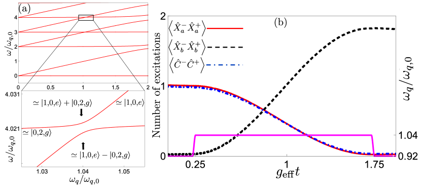
Figure 9: Two-photon frequency conversion via transitions between $|1,0,e\rangle$ and $|0,2,g\rangle$. (a) The energy levels of our system, given in Eq. (6), plotted as a function of the qubit frequency $\omega_{q}$, using the parameters $g_{a}=g_{b}=0.125\omega_{q,0}$, $\omega_{a}=3\omega_{q,0}$, and $\omega_{b}=2\omega_{q,0}$, where the reference point $\omega_{q,0}$ is set such that $\omega_{a}+\omega_{q,0}=2\omega_{b}$. In the zoom-in, close to the resonance $\omega_{a}+\omega_{q}=2\omega_{b}$, we see the anticrossing between $|1,0,e\rangle$ and $|0,2,g\rangle$ with the splitting $2g_{\rm eff}$ given by Eq. (11). Up-conversion of a photon pair into a single photon, or down-conversion of a single photon into a photon pair, can be achieved by adiabatically tuning $\omega_{q}$ to follow one of the energy levels in the figure from $|0,2,g\rangle$ to $|1,0,e\rangle$, or vice versa. (b) A rapid frequency conversion can be achieved by starting in $|1,0,e\rangle$ or $|0,2,g\rangle$, far from the resonance $\omega_{a}+\omega_{q}=2\omega_{b}$, tuning the qubit frequency (pink solid line) into resonance for half a Rabi period ($\pi/2g_{\rm eff}$) and then tuning it out of resonance again. The figure shows the number of excitations in the two resonators (red solid line for $a$, black dashed-dotted line for $b$) and the qubit (blue dashed line) during such a process, including decoherence in the form of relaxation from the resonators and the qubit. The parameters used for the decoherence are $\kappa_{a}=\kappa_{b}=\gamma=4\times 10^{-5}\omega_{q,0}$.

The two-photon frequency conversion can again be performed either by adiabatic transfer or by tuning the qubit into resonance for half a Rabi oscillation period, as explained in Sec. III. The energy levels to follow in the first approach are plotted in Fig. 9(a) and a simulation of the second approach, including decoherence, is shown in Fig. 9(b).

IV.2.2 Jaynes–Cummings Hamiltonian

For completeness, we calculate the effective coupling using only the JC Hamiltonian for two resonators and one qubit, i.e., we eliminate the non-excitation-conserving terms in the quantum Rabi Hamiltonian of Eq. (6) using the RWA, giving

$$\hat{H}_{\rm JC} = \omega_{a}\hat{a}^{\dagger}\hat{a}+\omega_{b}\hat{b}^{\dagger}\hat{b}+\frac{\omega_{q}}{2}\hat{\sigma}_{z}$$ (12)

$$+g_{a}\left(\hat{a}\hat{\sigma}_{+}+\hat{a}^{\dagger}\hat{\sigma}_{-}\right)+g_{b}\left(\hat{b}\hat{\sigma}_{+}+\hat{b}^{\dagger}\hat{\sigma}_{-}\right).$$

Retaining only the states connected by solid arrows in Fig. 8, we can write the Hamiltonian from Eq. (12) on matrix form as

$$\hat{H}_{\rm JC}=\begin{pmatrix}\omega_{b}+\frac{\omega_{q}}{2}&0&\sqrt{2}g_{b}&g_{a}\\ 0&\omega_{a}+\frac{\omega_{q}}{2}&0&g_{b}\\ \sqrt{2}g_{b}&0&2\omega_{b}-\frac{\omega_{q}}{2}&0\\ g_{a}&g_{b}&0&\omega_{a}+\omega_{b}-\frac{\omega_{q}}{2}\end{pmatrix},$$

(13)

where the states are ordered as $|0,1,e\rangle$, $|1,0,e\rangle$, $|0,2,g\rangle$, and $|1,1,g\rangle$. Again, we perform adiabatic elimination close to the resonance $\omega_{a}+\omega_{q}\approx 2\omega_{b}$. The details of the elimination are given in Appendix A.3.2. The result is an effective coupling between the states $|1,0,e\rangle$ and $|0,2,g\rangle$ with magnitude

$$g_{\rm eff}=-\frac{\sqrt{2}g_{a}g_{b}^{2}}{g_{a}^{2}+(\omega_{a}-\omega_{b})^{2}}$$ (14)

on resonance. Just as for the other two-photon frequency-conversion processes, the coupling scales like $g^{3}/\omega^{2}$ to leading order. In fact, Eq. (14) is a good approximation to Eq. (11), since the path given by the JC terms (solid lines) in Fig. 8 is far less detuned in energy from the initial and final states than all the other paths and thus gives the largest contribution to the result in Eq. (11). The remarks on the limit $\omega_{a}\to\omega_{b}$ given in Sec. IV.2.1 apply here as well. The schemes for implementing the frequency conversion are already given in Fig. 9.

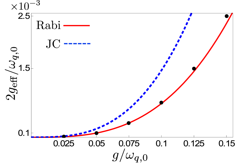
Figure 10: Comparison of analytical (JC Hamiltonian [dashed blue line] and quantum Rabi Hamiltonian [solid red line]) and numerical (black dots) results for the effective coupling between the states $|1,0,e\rangle$ and $|0,2,g\rangle$. The graph shows the minimum energy splitting $2g_{\rm eff}/\omega_{q,0}$ as a function of $g/\omega_{q,0}$, using the same parameters as in Fig. 9.

In Fig. 10, we compare the results from Eqs. (11) and (14) with a full numerical calculation. The contribution from the JC part dominates the coupling up until around $g_{a}=g_{b}=g=0.03\omega_{q,0}$ and gives a good approximation until then. For higher values of the coupling, using the approximation from the quantum Rabi Hamiltonian instead works fine up until around $g_{a}=g_{b}=g=0.15\omega_{q,0}$.

V Summary and outlook

We have shown how a system consisting of two resonators ultrastrongly coupled to a qubit can be used to realize a variety of frequency-conversion processes. In particular, we have shown how to convert a single photon into another photon of either higher or lower frequency, as well as how to convert a single photon into a photon pair and vice versa. All these processes are deterministic, can be implemented within a single setup, and do not require any external drives. The conversion is controlled by tuning the frequency of the qubit to and from values that make the desired transitions resonant.

Given the recent advances in USC circuit QED, we believe that our proposal can be implemented in such a setup. Indeed, two resonators have already been ultrastrongly coupled to a superconducting flux qubit Baust et al. (2016). Also, our proposal does not require very high coupling strengths. We only need that $g^{2}/\omega$ is appreciable (larger than the relevant decoherence rates) to realize single-photon frequency conversion; multi-photon frequency conversion can be demonstrated if $g^{3}/\omega^{2}$ is large enough.

A straightforward extension of the current work is to extend the calculations to processes with more photons in the second resonator or to add more resonators to the setup. Some of these possibilities are discussed in Ref. Kockum et al. (2017), where we explore analogies of nonlinear optics in USC systems, including the fact that the processes in the current work can be considered analogies of Raman and hyper-Raman scattering if the qubit is thought of as playing the role of a phonon. More general three-wave mixing, such as $|1,0,0,e\rangle\leftrightarrow|0,1,1,g\rangle$, or third-harmonic and -subharmonic generation such as $|1,0,e\rangle\leftrightarrow|0,3,g\rangle$, are examples of schemes that can be considered, but it must be kept in mind that higher-order processes with more photons involved will have lower effective coupling strengths. Another direction for future work is to investigate how the precise qubit control of the frequency-conversion processes discussed here can be used to prepare photon bundles Sánchez Muñoz et al. (2014) or interesting quantum superposition states with photons of different frequencies, a topic currently being explored in several frequency ranges Chirolli et al. (2010); Zakka-Bajjani et al. (2011); Clemmen et al. (2016).

Appendix A Analytical calculations of conversion rates

In this appendix, we present the full adiabatic-elimination calculations for the effective couplings in the three processes considered in this article: $|1,0,g\rangle\leftrightarrow|0,1,e\rangle$, $|1,0,g\rangle\leftrightarrow|0,2,e\rangle$, and $|1,0,e\rangle\leftrightarrow|0,2,g\rangle$. For each case, we compare the analytical results with numerical simulations to determine in what parameter regimes the analytical calculations constitute a good approximation.

A.1 $|1,0,g\rangle\leftrightarrow|0,1,e\rangle$

Starting from the truncated Hamiltonian in Eq. (3), we move to a frame rotating with $(\omega_{a}-\frac{\omega_{q}}{2})$, i.e., subtracting $(\omega_{a}-\frac{\omega_{q}}{2})$ from the diagonal of the Hamiltonian, giving

$$\hat{H}=\begin{pmatrix}-\omega_{a}&0&-g_{a}\sin\theta&g_{b}\cos\theta&0&0\\ 0&-(\omega_{a}-\omega_{q})&g_{a}\cos\theta&g_{b}\sin\theta&0&0\\ -g_{a}\sin\theta&g_{a}\cos\theta&0&0&-g_{b}\sin\theta&g_{b}\cos\theta\\ g_{b}\cos\theta&g_{b}\sin\theta&0&\omega_{b}+\omega_{q}-\omega_{a}&g_{a}\cos\theta&g_{a}\sin\theta\\ 0&0&-g_{b}\sin\theta&g_{a}\cos\theta&\omega_{b}&0\\ 0&0&g_{b}\cos\theta&g_{a}\sin\theta&0&\omega_{b}+\omega_{q}\end{pmatrix}.$$ (15)

Denoting the amplitudes of the six states by $c_{1}$–$c_{6}$, respectively, the Schrödinger equation gives

$$i\dot{c}_{1} = -\omega_{a}c_{1}-g_{a}\sin\theta c_{3}+g_{b}\cos\theta c_{4},$$ (16)

$$i\dot{c}_{2} = -(\omega_{a}-\omega_{q})c_{2}+g_{a}\cos\theta c_{3}+g_{b}\sin\theta c_{4},$$ (17)

$$i\dot{c}_{3} = -g_{a}\sin\theta c_{1}+g_{a}\cos\theta c_{2}-g_{b}\sin\theta c_{5}$$ (18)

$$+g_{b}\cos\theta c_{6},$$

$$i\dot{c}_{4} = (\omega_{b}+\omega_{q}-\omega_{a})c_{4}+g_{b}\cos\theta c_{1}+g_{b}\sin\theta c_{2}$$ (19)

$$+g_{a}\cos\theta c_{5}+g_{a}\sin\theta c_{6},$$

$$i\dot{c}_{5} = \omega_{b}c_{5}-g_{b}\sin\theta c_{3}+g_{a}\cos\theta c_{4},$$ (20)

$$i\dot{c}_{6} = (\omega_{b}+\omega_{q})c_{6}+g_{b}\cos\theta c_{3}+g_{a}\sin\theta c_{4}.$$ (21)

Assuming that $\omega_{a}\approx\omega_{b}+\omega_{q}$, and that $g_{a},g_{b}\ll\omega_{a},\omega_{b},\left|\omega_{a}-\omega_{q}\right|,\omega_{b}+\omega_{q}$, we can adiabatically eliminate the four intermediate levels (their population will not change significantly), i.e., set $\dot{c}_{1}=\dot{c}_{2}=\dot{c}_{5}=\dot{c}_{6}=0$. This gives

$$c_{1} = -\frac{g_{a}\sin\theta}{\omega_{a}}c_{3}+\frac{g_{b}\cos\theta}{\omega_{a}}c_{4},$$ (22)

$$c_{2} = \frac{g_{a}\cos\theta}{\omega_{a}-\omega_{q}}c_{3}+\frac{g_{b}\sin\theta}{\omega_{a}-\omega_{q}}c_{4},$$ (23)

$$c_{5} = \frac{g_{b}\sin\theta}{\omega_{b}}c_{3}-\frac{g_{a}\cos\theta}{\omega_{b}}c_{4},$$ (24)

$$c_{6} = -\frac{g_{b}\cos\theta}{\omega_{b}+\omega_{q}}c_{3}-\frac{g_{a}\sin\theta}{\omega_{b}+\omega_{q}}c_{4},$$ (25)

which we then insert into the equations for $c_{3}$ and $c_{4}$ to arrive at

$$i\dot{c}_{3} = \left(\frac{g_{a}^{2}\sin^{2}\theta}{\omega_{a}}+\frac{g_{a}^{2}\cos^{2}\theta}{\omega_{a}-\omega_{q}}-\frac{g_{b}^{2}\sin^{2}\theta}{\omega_{b}}-\frac{g_{b}^{2}\cos^{2}\theta}{\omega_{b}+\omega_{q}}\right)c_{3}$$ (26)

$$+\frac{1}{2}g_{a}g_{b}\sin 2\theta$$

$$\times\left(\frac{1}{\omega_{a}-\omega_{q}}+\frac{1}{\omega_{b}}-\frac{1}{\omega_{a}}-\frac{1}{\omega_{b}+\omega_{q}}\right)c_{4},$$

$$i\dot{c}_{4} = \frac{1}{2}g_{a}g_{b}\sin 2\theta\left(\frac{1}{\omega_{a}-\omega_{q}}+\frac{1}{\omega_{b}}-\frac{1}{\omega_{a}}-\frac{1}{\omega_{b}+\omega_{q}}\right)c_{3}$$ (27)

$$+\bigg{(}\omega_{b}+\omega_{q}-\omega_{a}+\frac{g_{b}^{2}\cos^{2}\theta}{\omega_{a}}+\frac{g_{b}^{2}\sin^{2}\theta}{\omega_{a}-\omega_{q}}$$

$$-\frac{g_{a}^{2}\cos^{2}\theta}{\omega_{b}}-\frac{g_{a}\sin\theta}{\omega_{b}+\omega_{q}}\bigg{)}c_{4}.$$

While the energy level shifts in these equations are not final (they can be affected by processes involving more energy levels), the effective coupling rate between $|1,0,g\rangle$ and $|0,1,e\rangle$ is shown to be

$$g_{\rm eff}=\frac{1}{2}g_{a}g_{b}\sin 2\theta\left(\frac{1}{\omega_{a}-\omega_{q}}+\frac{1}{\omega_{b}}-\frac{1}{\omega_{a}}-\frac{1}{\omega_{b}+\omega_{q}}\right).$$ (28)

Assuming that we are exactly on resonance, the qubit frequency can be eliminated from this expression using $\omega_{q}=\omega_{a}-\omega_{b}$, leading to

$$g_{\rm eff}=g_{a}g_{b}\sin 2\theta\left(\frac{1}{\omega_{b}}-\frac{1}{\omega_{a}}\right)=\frac{g_{a}g_{b}(\omega_{a}-\omega_{b})\sin 2\theta}{\omega_{a}\omega_{b}},$$ (29)

the first part of which is given in Eq. (5). We note that the result agrees with the perturbation-theory calculations performed in Ref. Kockum et al. (2017). In general, the adiabatic elimination is more exact, but for a second-order process the result for the effective coupling is the same with both methods.

A.2 $|1,0,g\rangle\leftrightarrow|0,2,e\rangle$

Starting from the truncated Hamiltonian in Eq. (7), we move to a frame rotating with $(\omega_{a}-\frac{\omega_{q}}{2})$, i.e., subtracting $(\omega_{a}-\frac{\omega_{q}}{2})$ from the diagonal of the Hamiltonian, giving

$$\hat{H}_{\rm R}=\begin{pmatrix}\omega_{q}-\omega_{a}&g_{b}&g_{a}&0&0&0\\ g_{b}&\omega_{b}-\omega_{a}&0&\sqrt{2}g_{b}&g_{a}&0\\ g_{a}&0&0&0&g_{b}&0\\ 0&\sqrt{2}g_{b}&0&2\omega_{b}-\omega_{a}+\omega_{q}&0&g_{a}\\ 0&g_{a}&g_{b}&0&\omega_{b}+\omega_{q}&\sqrt{2}g_{b}\\ 0&0&0&g_{a}&\sqrt{2}g_{b}&2\omega_{b}\end{pmatrix}.$$ (30)

Denoting the amplitudes of the six states by $c_{1}$–$c_{6}$, the Schrödinger equation gives

$$i\dot{c}_{1} = (\omega_{q}-\omega_{a})c_{1}+g_{b}c_{2}+g_{a}c_{3},$$ (31)

$$i\dot{c}_{2} = (\omega_{b}-\omega_{a})c_{2}+g_{b}c_{1}+\sqrt{2}g_{b}c_{4}+g_{a}c_{5},$$ (32)

$$i\dot{c}_{3} = g_{a}c_{1}+g_{b}c_{5},$$ (33)

$$i\dot{c}_{4} = (2\omega_{b}-\omega_{a}+\omega_{q})c_{4}+\sqrt{2}g_{b}c_{2}+g_{a}c_{6},$$ (34)

$$i\dot{c}_{5} = (\omega_{b}+\omega_{q})c_{5}+g_{a}c_{2}+g_{b}c_{3}+\sqrt{2}g_{b}c_{6},$$ (35)

$$i\dot{c}_{6} = 2\omega_{b}c_{6}+g_{a}c_{4}+\sqrt{2}g_{b}c_{5}.$$ (36)

Assuming that $\omega_{a}\approx 2\omega_{b}+\omega_{q}$, and that $g_{a},g_{b}\ll\omega_{b}+\omega_{q},\left|\omega_{b}-\omega_{q}\right|,\left|\omega_{a}-\omega_{q}\right|$, we can adiabatically eliminate the four intermediate levels, i.e., set $\dot{c}_{1}=\dot{c}_{2}=\dot{c}_{5}=\dot{c}_{6}=0$. This gives

$$i\dot{c}_{3} = \frac{g_{a}^{4}\omega_{b}+g_{a}^{2}\left[\omega_{b}(\omega_{a}-\omega_{b})^{2}-g_{b}^{2}(\omega_{a}+\omega_{b})\right]+g_{b}^{2}\omega_{b}\left[g_{b}^{2}+2\omega_{b}(\omega_{b}-\omega_{a})\right]}{2\omega_{b}^{2}\left[g_{a}^{2}+(\omega_{a}-\omega_{b})^{2}\right]+g_{b}^{4}+3g_{b}^{2}\omega_{b}(\omega_{b}-\omega_{a})}c_{3}$$ (37)

$$+\frac{g_{a}g_{b}^{2}\left[g_{a}^{2}-3g_{b}^{2}+4\omega_{b}(\omega_{a}-2\omega_{b})\right]}{\sqrt{2}\left\{2\omega_{b}^{2}\left[g_{a}^{2}+(\omega_{a}-\omega_{b})^{2}\right]+g_{b}^{4}+3g_{b}^{2}\omega_{b}(\omega_{b}-\omega_{a})\right\}}c_{4},$$

where we simplified the expressions somewhat by setting $\omega_{q}=\omega_{a}-2\omega_{b}$. While the energy level shift in this equation is not final (they can be affected by processes involving more energy levels), the effective coupling rate between $|1,0,g\rangle$ and $|0,2,e\rangle$ is shown to be

$$g_{\rm eff}=\frac{g_{a}g_{b}^{2}\left[g_{a}^{2}-3g_{b}^{2}+4\omega_{b}(\omega_{a}-2\omega_{b})\right]}{\sqrt{2}\left\{2\omega_{b}^{2}\left[g_{a}^{2}+(\omega_{a}-\omega_{b})^{2}\right]+g_{b}^{4}+3g_{b}^{2}\omega_{b}(\omega_{b}-\omega_{a})\right\}}.$$ (38)

Setting $g_{a}=g_{b}\equiv g$, this reduces to

$$g_{\rm eff}=\frac{\sqrt{2}g^{3}\left[2\omega_{b}(\omega_{a}-2\omega_{b})-g^{2}\right]}{2\omega_{b}^{2}(\omega_{a}-\omega_{b})^{2}+g^{2}\omega_{b}(5\omega_{b}-3\omega_{a})+g^{4}},$$ (39)

which is Eq. (8). As shown in Fig. 7, this expression for the effective coupling is a good approximation to the exact value up to at least $g_{a}=g_{b}=g=0.3\omega_{q,0}$. We can simplify the expression for the coupling further by only keeping terms to leading order in $g/\omega$; the result is

$$g_{\rm eff}=\frac{\sqrt{2}g^{3}\left(\omega_{a}-2\omega_{b}\right)}{\omega_{b}\left(\omega_{a}-\omega_{b}\right)^{2}},$$ (40)

which is Eq. (9). This agrees with the perturbation-theory calculation in Ref. Kockum et al. (2017), which only captures the leading-order term.

A.3 $|1,0,e\rangle\leftrightarrow|0,2,g\rangle$

For the process $|1,0,e\rangle\leftrightarrow|0,2,g\rangle$, we perform adiabatic elimination starting from both the quantum Rabi Hamiltonian and the JC Hamiltonian.

A.3.1 Quantum Rabi Hamiltonian

Starting from the truncated Hamiltonian in Eq. (10), we move to a frame rotating with $(\omega_{a}+\frac{\omega_{q}}{2})$, i.e., subtracting $(\omega_{a}+\frac{\omega_{q}}{2})$ from the diagonal of the Hamiltonian, giving

$$\hat{H}_{\rm R}=\begin{pmatrix}-\omega_{a}-\omega_{q}&g_{b}&g_{a}&0&0&0\\ g_{b}&\omega_{b}-\omega_{a}&0&\sqrt{2}g_{b}&g_{a}&0\\ g_{a}&0&0&0&g_{b}&0\\ 0&\sqrt{2}g_{b}&0&2\omega_{b}-\omega_{a}-\omega_{q}&0&g_{a}\\ 0&g_{a}&g_{b}&0&\omega_{b}-\omega_{q}&\sqrt{2}g_{b}\\ 0&0&0&g_{a}&\sqrt{2}g_{b}&2\omega_{b}\end{pmatrix}.$$ (41)

Denoting the amplitudes of the six states by $c_{1}$–$c_{6}$, the Schrödinger equation gives

$$i\dot{c}_{1} = -(\omega_{a}+\omega_{q})c_{1}+g_{b}c_{2}+g_{a}c_{3},$$ (42)

$$i\dot{c}_{2} = (\omega_{b}-\omega_{a})c_{2}+g_{b}c_{1}+\sqrt{2}g_{b}c_{4}+g_{a}c_{5},$$ (43)

$$i\dot{c}_{3} = g_{a}c_{1}+g_{b}c_{5},$$ (44)

$$i\dot{c}_{4} = (2\omega_{b}-\omega_{a}-\omega_{q})c_{4}+\sqrt{2}g_{b}c_{2}+g_{a}c_{6},$$ (45)

$$i\dot{c}_{5} = (\omega_{b}-\omega_{q})c_{5}+g_{a}c_{2}+g_{b}c_{3}+\sqrt{2}g_{b}c_{6},$$ (46)

$$i\dot{c}_{6} = 2\omega_{b}c_{6}+g_{a}c_{4}+\sqrt{2}g_{b}c_{5}.$$ (47)

Assuming that $\omega_{a}+\omega_{q}\approx 2\omega_{b}$, and that $g_{a},g_{b}\ll\left|\omega_{b}-\omega_{q}\right|,\omega_{b}+\omega_{q},\omega_{a}+\omega_{q},\left|\omega_{a}-\omega_{q}\right|$, we can adiabatically eliminate the four intermediate levels, i.e., set $\dot{c}_{1}=\dot{c}_{2}=\dot{c}_{5}=\dot{c}_{6}=0$. This gives

$$i\dot{c}_{3} = \frac{g_{a}^{4}\omega_{b}+g_{a}^{2}\left[\omega_{b}(\omega_{a}-\omega_{b})^{2}-g_{b}^{2}(\omega_{a}+\omega_{b})\right]+g_{b}^{2}\omega_{b}\left[g_{b}^{2}+2\omega_{b}(\omega_{b}-\omega_{a})\right]}{2\omega_{b}^{2}\left[g_{a}^{2}+(\omega_{a}-\omega_{b})^{2}\right]+g_{b}^{4}+3g_{b}^{2}\omega_{b}(\omega_{b}-\omega_{a})}c_{3}$$ (48)

$$+\frac{g_{a}g_{b}^{2}\left[g_{a}^{2}-3g_{b}^{2}+4\omega_{b}(\omega_{a}-2\omega_{b})\right]}{\sqrt{2}\left\{2\omega_{b}^{2}\left[g_{a}^{2}+(\omega_{a}-\omega_{b})^{2}\right]+g_{b}^{4}+3g_{b}^{2}\omega_{b}(\omega_{b}-\omega_{a})\right\}}c_{4},$$

where we simplified the expressions somewhat by setting $\omega_{q}=2\omega_{b}-\omega_{a}$. While the energy level shift in this equation is not final (it can be affected by processes involving more energy levels), the effective coupling rate between $|1,0,e\rangle$ and $|0,2,g\rangle$ is shown to be

$$g_{\rm eff}=\frac{g_{a}g_{b}^{2}\left[g_{a}^{2}-3g_{b}^{2}+4\omega_{b}(\omega_{a}-2\omega_{b})\right]}{\sqrt{2}\left\{2\omega_{b}^{2}\left[g_{a}^{2}+(\omega_{a}-\omega_{b})^{2}\right]+g_{b}^{4}+3g_{b}^{2}\omega_{b}(\omega_{b}-\omega_{a})\right\}}.$$ (49)

Setting $g_{a}=g_{b}\equiv g$, this reduces to

$$g_{\rm eff}=\frac{\sqrt{2}g^{3}\left[2\omega_{b}(\omega_{a}-2\omega_{b})-g^{2}\right]}{2\omega_{b}^{2}(\omega_{a}-\omega_{b})^{2}+g^{2}\omega_{b}(5\omega_{b}-3\omega_{a})+g^{4}},$$ (50)

which is Eq. (11). As noted in the main text, this is equal to the coupling for the case $|1,0,g\rangle\leftrightarrow|0,2,e\rangle$, but other values of $\omega_{a}$ and $\omega_{b}$ are permitted in this case. In particular, the coupling can be increased by letting $\omega_{a}\to\omega_{b}$, but the approximations we have used here break down when $\left|\omega_{a}-\omega_{b}\right|$ becomes comparable to $g$. Again, the result agrees with the perturbation-theory calculation in Ref. Kockum et al. (2017), which only captures the leading-order term.

A.3.2 Jaynes–Cummings Hamiltonian

Starting from the truncated Hamiltonian in Eq. (13), we move to a frame rotating with $(\omega_{a}+\frac{\omega_{q}}{2})$, i.e., subtracting $(\omega_{a}+\frac{\omega_{q}}{2})$ from the diagonal of the Hamiltonian, giving

$$\hat{H}_{\rm JC}=\begin{pmatrix}\omega_{b}-\omega_{a}&0&\sqrt{2}g_{b}&g_{a}\\ 0&0&0&g_{b}\\ \sqrt{2}g_{b}&0&2\omega_{b}-\omega_{a}-\omega_{q}&0\\ g_{a}&g_{b}&0&\omega_{b}-\omega_{q}\end{pmatrix}.$$

Denoting the amplitudes of the four states by $c_{1}$–$c_{4}$, the Schrödinger equation gives

$$i\dot{c}_{1} = (\omega_{b}-\omega_{a})c_{1}+\sqrt{2}g_{b}c_{3}+g_{a}c_{4},$$ (52)

$$i\dot{c}_{2} = g_{b}c_{4},$$ (53)

$$i\dot{c}_{3} = (2\omega_{b}-\omega_{a}-\omega_{q})c_{3}+\sqrt{2}g_{b}c_{1},$$ (54)

$$i\dot{c}_{4} = (\omega_{b}-\omega_{q})c_{4}+g_{a}c_{1}+g_{b}c_{2}.$$ (55)

Assuming that $\omega_{a}+\omega_{q}\approx 2\omega_{b}$, and that $g_{a},g_{b}\ll\omega_{a},\omega_{b},\omega_{q}$, we can adiabatically eliminate the two intermediate levels, i.e., set $\dot{c}_{1}=\dot{c}_{4}=0$. This gives

$$i\dot{c}_{2} = -\frac{g_{b}^{2}(\omega_{a}-\omega_{b})}{g_{a}^{2}+(\omega_{a}-\omega_{b})^{2}}c_{2}-\frac{\sqrt{2}g_{a}g_{b}^{2}}{g_{a}^{2}+(\omega_{a}-\omega_{b})^{2}}c_{3},\quad\quad$$ (56)

where we set $\omega_{q}=2\omega_{b}-\omega_{a}$. While the energy level shift in this equation is not final (it can be affected by processes involving more energy levels), the effective coupling rate between $|1,0,e\rangle$ and $|0,2,g\rangle$ is shown to be

$$g_{\rm eff}=-\frac{\sqrt{2}g_{a}g_{b}^{2}}{g_{a}^{2}+(\omega_{a}-\omega_{b})^{2}},$$ (57)

which is Eq. (14). Setting $g_{a}=g_{b}\equiv g$, this reduces to

$$g_{\rm eff}=-\frac{\sqrt{2}g^{3}}{g^{2}+(\omega_{a}-\omega_{b})^{2}},$$ (58)

which to leading order in $g/\omega$ becomes

$$g_{\rm eff}=-\frac{\sqrt{2}g^{3}}{\left(\omega_{a}-\omega_{b}\right)^{2}},$$ (59)

agreeing with the perturbation-theory calculation of Ref. Kockum et al. (2017).

References

- Kumar (1990) P. Kumar, “Quantum frequency conversion,” Optics Letters 15, 1476 (1990).
- Huang and Kumar (1992) J. Huang and P. Kumar, “Observation of quantum frequency conversion,” Physical Review Letters 68, 2153 (1992).
- O’Brien et al. (2009) J. L. O’Brien, A. Furusawa, and J. Vučković, “Photonic quantum technologies,” Nature Photonics 3, 687 (2009), arXiv:1003.3928 .
- Buluta et al. (2011) I. Buluta, S. Ashhab, and F. Nori, “Natural and artificial atoms for quantum computation,” Reports on Progress in Physics 74, 104401 (2011), arXiv:1002.1871 .
- Kimble (2008) H. J. Kimble, “The quantum internet,” Nature 453, 1023 (2008), arXiv:0806.4195 .
- Albota and Wong (2004) M. A. Albota and F. N. C. Wong, “Efficient single-photon counting at 155 m by means of frequency upconversion,” Optics Letters 29, 1449 (2004).
- Tanzilli et al. (2005) S. Tanzilli, W. Tittel, M. Halder, O. Alibart, P. Baldi, N. Gisin, and H. Zbinden, “A photonic quantum information interface,” Nature 437, 116 (2005), arXiv:0509011 [quant-ph] .
- Ou (2008) Z. Y. Ou, “Efficient conversion between photons and between photon and atom by stimulated emission,” Physical Review A 78, 023819 (2008).
- Ding and Ou (2010) Y. Ding and Z. Y. Ou, “Frequency downconversion for a quantum network,” Optics Letters 35, 2591 (2010), arXiv:1007.5375 .
- Takesue (2010) H. Takesue, “Single-photon frequency down-conversion experiment,” Physical Review A 82, 013833 (2010), arXiv:1006.0364 .
- Guo et al. (2016) X. Guo, C.-L. Zou, H. Jung, and H. X. Tang, “On-Chip Strong Coupling and Efficient Frequency Conversion between Telecom and Visible Optical Modes,” Physical Review Letters 117, 123902 (2016), arXiv:1511.08112 .
- You and Nori (2011) J. Q. You and F. Nori, “Atomic physics and quantum optics using superconducting circuits,” Nature 474, 589 (2011), arXiv:1202.1923 .
- Devoret and Schoelkopf (2013) M. H. Devoret and R. J. Schoelkopf, “Superconducting Circuits for Quantum Information: An Outlook,” Science 339, 1169 (2013).
- Bochmann et al. (2013) J. Bochmann, A. Vainsencher, D. D. Awschalom, and A. N. Cleland, “Nanomechanical coupling between microwave and optical photons,” Nature Physics 9, 712 (2013).
- Andrews et al. (2014) R. W. Andrews, R. W. Peterson, T. P. Purdy, K. Cicak, R. W. Simmonds, C. A. Regal, and K. W. Lehnert, “Bidirectional and efficient conversion between microwave and optical light,” Nature Physics 10, 321 (2014), arXiv:1310.5276 .
- Shumeiko (2016) V. S. Shumeiko, “Quantum acousto-optic transducer for superconducting qubits,” Physical Review A 93, 023838 (2016), arXiv:1511.03819 .
- Hisatomi et al. (2016) R. Hisatomi, A. Osada, Y. Tabuchi, T. Ishikawa, A. Noguchi, R. Yamazaki, K. Usami, and Y. Nakamura, “Bidirectional conversion between microwave and light via ferromagnetic magnons,” Physical Review B 93, 174427 (2016), arXiv:1601.03908 .
- You and Nori (2003) J. Q. You and F. Nori, “Quantum information processing with superconducting qubits in a microwave field,” Physical Review B 68, 064509 (2003), arXiv:0306207 [cond-mat] .
- Wallraff et al. (2004) A. Wallraff, D. I. Schuster, A. Blais, L. Frunzio, R.-S. Huang, J. Majer, S. Kumar, S. M. Girvin, and R. J. Schoelkopf, “Strong coupling of a single photon to a superconducting qubit using circuit quantum electrodynamics,” Nature 431, 162 (2004), arXiv:0407325 [cond-mat] .
- Blais et al. (2004) A. Blais, R.-S. Huang, A. Wallraff, S. M. Girvin, and R. J. Schoelkopf, “Cavity quantum electrodynamics for superconducting electrical circuits: An architecture for quantum computation,” Physical Review A 69, 062320 (2004), arXiv:0402216 [cond-mat] .
- Xiang et al. (2013) Z.-L. Xiang, S. Ashhab, J. Q. You, and F. Nori, “Hybrid quantum circuits: Superconducting circuits interacting with other quantum systems,” Reviews of Modern Physics 85, 623 (2013), arXiv:1204.2137 .
- Wallquist et al. (2006) M. Wallquist, V. S. Shumeiko, and G. Wendin, “Selective coupling of superconducting charge qubits mediated by a tunable stripline cavity,” Physical Review B 74, 224506 (2006), arXiv:0608209 [cond-mat] .
- Sandberg et al. (2008) M. Sandberg, C. M. Wilson, F. Persson, T. Bauch, G. Johansson, V. Shumeiko, T. Duty, and P. Delsing, “Tuning the field in a microwave resonator faster than the photon lifetime,” Applied Physics Letters 92, 203501 (2008), arXiv:0801.2479 .
- Johansson et al. (2010) J. R. Johansson, G. Johansson, C. M. Wilson, and F. Nori, “Dynamical Casimir effect in superconducting microwave circuits,” Physical Review A 82, 52509 (2010), arXiv:1007.1058 .
- Chirolli et al. (2010) L. Chirolli, G. Burkard, S. Kumar, and D. P. DiVincenzo, “Superconducting Resonators as Beam Splitters for Linear-Optics Quantum Computation,” Physical Review Letters 104, 230502 (2010), arXiv:1002.1394 .
- Zakka-Bajjani et al. (2011) E. Zakka-Bajjani, F. Nguyen, M. Lee, L. R. Vale, R. W. Simmonds, and J. Aumentado, “Quantum superposition of a single microwave photon in two different ’colour’ states,” Nature Physics 7, 599 (2011), arXiv:1106.2523 .
- Abdo et al. (2013) B. Abdo, K. Sliwa, F. Schackert, N. Bergeal, M. Hatridge, L. Frunzio, A. D. Stone, and M. Devoret, “Full Coherent Frequency Conversion between Two Propagating Microwave Modes,” Physical Review Letters 110, 173902 (2013), arXiv:1212.2231 .
- Kamal et al. (2014) A. Kamal, A. Roy, J. Clarke, and M. H. Devoret, “Asymmetric Frequency Conversion in Nonlinear Systems Driven by a Biharmonic Pump,” Physical Review Letters 113, 247003 (2014), arXiv:1405.1745 .
- Marquardt (2007) F. Marquardt, “Efficient on-chip source of microwave photon pairs in superconducting circuit QED,” Physical Review B 76, 205416 (2007), arXiv:0605232 [cond-mat] .
- Koshino (2009) K. Koshino, “Down-conversion of a single photon with unit efficiency,” Physical Review A 79, 013804 (2009).
- Sánchez-Burillo et al. (2016) E. Sánchez-Burillo, L. Martín-Moreno, J. J. García-Ripoll, and D. Zueco, “Full two-photon down-conversion of a single photon,” Physical Review A 94, 053814 (2016), arXiv:1602.05603 .
- Inomata et al. (2014) K. Inomata, K. Koshino, Z. R. Lin, W. D. Oliver, J. S. Tsai, Y. Nakamura, and T. Yamamoto, “Microwave Down-Conversion with an Impedance-Matched System in Driven Circuit QED,” Physical Review Letters 113, 063604 (2014), arXiv:1405.5592 .
- Deppe et al. (2008) F. Deppe, M. Mariantoni, E. P. Menzel, A. Marx, S. Saito, K. Kakuyanagi, H. Tanaka, T. Meno, K. Semba, H. Takayanagi, E. Solano, and R. Gross, “Two-photon probe of the Jaynes–Cummings model and controlled symmetry breaking in circuit QED,” Nature Physics 4, 686 (2008), arXiv:0805.3294 .
- Liu et al. (2005) Y.-X. Liu, J. Q. You, L. F. Wei, C. P. Sun, and F. Nori, “Optical Selection Rules and Phase-Dependent Adiabatic State Control in a Superconducting Quantum Circuit,” Physical Review Letters 95, 087001 (2005), arXiv:0501047 [quant-ph] .
- Liu et al. (2014) Y.-X. Liu, H.-C. Sun, Z. H. Peng, A. Miranowicz, J. S. Tsai, and F. Nori, “Controllable microwave three-wave mixing via a single three-level superconducting quantum circuit,” Scientific Reports 4, 7289 (2014), arXiv:1308.6409 .
- Lecocq et al. (2016) F. Lecocq, J. B. Clark, R. W. Simmonds, J. Aumentado, and J. D. Teufel, “Mechanically Mediated Microwave Frequency Conversion in the Quantum Regime,” Physical Review Letters 116, 043601 (2016), arXiv:1512.00078 .
- Günter et al. (2009) G. Günter, A. A. Anappara, J. Hees, A. Sell, G. Biasiol, L. Sorba, S. De Liberato, C. Ciuti, A. Tredicucci, A. Leitenstorfer, and R. Huber, “Sub-cycle switch-on of ultrastrong light–matter interaction,” Nature 458, 178 (2009).
- Forn-Díaz et al. (2010) P. Forn-Díaz, J. Lisenfeld, D. Marcos, J. J. García-Ripoll, E. Solano, C. J. P. M. Harmans, and J. E. Mooij, “Observation of the Bloch-Siegert Shift in a Qubit-Oscillator System in the Ultrastrong Coupling Regime,” Physical Review Letters 105, 237001 (2010), arXiv:1005.1559 .
- Niemczyk et al. (2010) T. Niemczyk, F. Deppe, H. Huebl, E. P. Menzel, F. Hocke, M. J. Schwarz, J. J. Garcia-Ripoll, D. Zueco, T. Hümmer, E. Solano, A. Marx, and R. Gross, “Circuit quantum electrodynamics in the ultrastrong-coupling regime,” Nature Physics 6, 772 (2010), arXiv:1003.2376 .
- Todorov et al. (2010) Y. Todorov, A. M. Andrews, R. Colombelli, S. De Liberato, C. Ciuti, P. Klang, G. Strasser, and C. Sirtori, “Ultrastrong Light-Matter Coupling Regime with Polariton Dots,” Physical Review Letters 105, 196402 (2010), arXiv:1301.1297 .
- Schwartz et al. (2011) T. Schwartz, J. A. Hutchison, C. Genet, and T. W. Ebbesen, “Reversible Switching of Ultrastrong Light-Molecule Coupling,” Physical Review Letters 106, 196405 (2011).
- Scalari et al. (2012) G. Scalari, C. Maissen, D. Turcinkova, D. Hagenmuller, S. De Liberato, C. Ciuti, C. Reichl, D. Schuh, W. Wegscheider, M. Beck, and J. Faist, “Ultrastrong Coupling of the Cyclotron Transition of a 2D Electron Gas to a THz Metamaterial,” Science 335, 1323 (2012), arXiv:1111.2486 .
- Geiser et al. (2012) M. Geiser, F. Castellano, G. Scalari, M. Beck, L. Nevou, and J. Faist, “Ultrastrong Coupling Regime and Plasmon Polaritons in Parabolic Semiconductor Quantum Wells,” Physical Review Letters 108, 106402 (2012), arXiv:1111.7266 .
- Kéna-Cohen et al. (2013) S. Kéna-Cohen, S. A. Maier, and D. D. C. Bradley, “Ultrastrongly Coupled Exciton-Polaritons in Metal-Clad Organic Semiconductor Microcavities,” Advanced Optical Materials 1, 827 (2013).
- Gambino et al. (2014) S. Gambino, M. Mazzeo, A. Genco, O. Di Stefano, S. Savasta, S. Patanè, D. Ballarini, F. Mangione, G. Lerario, D. Sanvitto, and G. Gigli, “Exploring Light–Matter Interaction Phenomena under Ultrastrong Coupling Regime,” ACS Photonics 1, 1042 (2014).
- Maissen et al. (2014) C. Maissen, G. Scalari, F. Valmorra, M. Beck, J. Faist, S. Cibella, R. Leoni, C. Reichl, C. Charpentier, and W. Wegscheider, “Ultrastrong coupling in the near field of complementary split-ring resonators,” Physical Review B 90, 205309 (2014), arXiv:1408.3547 .
- Goryachev et al. (2014) M. Goryachev, W. G. Farr, D. L. Creedon, Y. Fan, M. Kostylev, and M. E. Tobar, “High-Cooperativity Cavity QED with Magnons at Microwave Frequencies,” Physical Review Applied 2, 054002 (2014), arXiv:1408.2905 .
- Baust et al. (2016) A. Baust, E. Hoffmann, M. Haeberlein, M. J. Schwarz, P. Eder, J. Goetz, F. Wulschner, E. Xie, L. Zhong, F. Quijandría, D. Zueco, J.-J. García Ripoll, L. García-Álvarez, G. Romero, E. Solano, K. G. Fedorov, E. P. Menzel, F. Deppe, A. Marx, and R. Gross, “Ultrastrong coupling in two-resonator circuit QED,” Physical Review B 93, 214501 (2016), arXiv:1412.7372 .
- Forn-Díaz et al. (2017) P. Forn-Díaz, J. J. García-Ripoll, B. Peropadre, J.-L. Orgiazzi, M. A. Yurtalan, R. Belyansky, C. M. Wilson, and A. Lupascu, “Ultrastrong coupling of a single artificial atom to an electromagnetic continuum in the nonperturbative regime,” Nature Physics 13, 39 (2017), arXiv:1602.00416 .
- Yoshihara et al. (2017) F. Yoshihara, T. Fuse, S. Ashhab, K. Kakuyanagi, S. Saito, and K. Semba, “Superconducting qubit-oscillator circuit beyond the ultrastrong-coupling regime,” Nature Physics 13, 44 (2017), arXiv:1602.00415 .
- Chen et al. (2016) Z. Chen, Y. Wang, T. Li, L. Tian, Y. Qiu, K. Inomata, F. Yoshihara, S. Han, F. Nori, J. S. Tsai, and J. Q. You, “Multi-photon sideband transitions in an ultrastrongly-coupled circuit quantum electrodynamics system,” (2016), arXiv:1602.01584 .
- George et al. (2016) J. George, T. Chervy, A. Shalabney, E. Devaux, H. Hiura, C. Genet, and T. W. Ebbesen, “Multiple Rabi Splittings under Ultrastrong Vibrational Coupling,” Physical Review Letters 117, 153601 (2016), arXiv:1609.01520 .
- Langford et al. (2016) N. K. Langford, R. Sagastizabal, M. Kounalakis, C. Dickel, A. Bruno, F. Luthi, D. J. Thoen, A. Endo, and L. DiCarlo, “Experimentally simulating the dynamics of quantum light and matter at ultrastrong coupling,” (2016), arXiv:1610.10065 .
- Braumüller et al. (2016) J. Braumüller, M. Marthaler, A. Schneider, A. Stehli, H. Rotzinger, M. Weides, and A. V. Ustinov, “Analog quantum simulation of the Rabi model in the ultra-strong coupling regime,” (2016), arXiv:1611.08404 .
- Yoshihara et al. (2016) F. Yoshihara, T. Fuse, S. Ashhab, K. Kakuyanagi, S. Saito, and K. Semba, “Characteristic spectra of circuit quantum electrodynamics systems from the ultrastrong to the deep strong coupling regime,” (2016), arXiv:1612.00121 .
- De Liberato et al. (2007) S. De Liberato, C. Ciuti, and I. Carusotto, “Quantum Vacuum Radiation Spectra from a Semiconductor Microcavity with a Time-Modulated Vacuum Rabi Frequency,” Physical Review Letters 98, 103602 (2007), arXiv:0611282 [cond-mat] .
- Ashhab and Nori (2010) S. Ashhab and F. Nori, “Qubit-oscillator systems in the ultrastrong-coupling regime and their potential for preparing nonclassical states,” Physical Review A 81, 042311 (2010), arXiv:0912.4888 .
- Cao et al. (2010) X. Cao, J. Q. You, H. Zheng, A. G. Kofman, and F. Nori, “Dynamics and quantum Zeno effect for a qubit in either a low- or high-frequency bath beyond the rotating-wave approximation,” Physical Review A 82, 022119 (2010), arXiv:1001.4831 .
- Cao et al. (2011) X. Cao, J. Q. You, H. Zheng, and F. Nori, “A qubit strongly coupled to a resonant cavity: asymmetry of the spontaneous emission spectrum beyond the rotating wave approximation,” New Journal of Physics 13, 073002 (2011), arXiv:1009.4366 .
- Stassi et al. (2013) R. Stassi, A. Ridolfo, O. Di Stefano, M. J. Hartmann, and S. Savasta, “Spontaneous Conversion from Virtual to Real Photons in the Ultrastrong-Coupling Regime,” Physical Review Letters 110, 243601 (2013), arXiv:1210.2367 .
- Sanchez-Burillo et al. (2014) E. Sanchez-Burillo, D. Zueco, J. J. Garcia-Ripoll, and L. Martin-Moreno, “Scattering in the Ultrastrong Regime: Nonlinear Optics with One Photon,” Physical Review Letters 113, 263604 (2014), arXiv:1406.5779 .
- De Liberato (2014) S. De Liberato, “Light-Matter Decoupling in the Deep Strong Coupling Regime: The Breakdown of the Purcell Effect,” Physical Review Letters 112, 016401 (2014), arXiv:1308.2812 .
- Lolli et al. (2015) J. Lolli, A. Baksic, D. Nagy, V. E. Manucharyan, and C. Ciuti, “Ancillary Qubit Spectroscopy of Vacua in Cavity and Circuit Quantum Electrodynamics,” Physical Review Letters 114, 183601 (2015), arXiv:1411.5618 .
- Di Stefano et al. (2016) O. Di Stefano, R. Stassi, L. Garziano, A. F. Kockum, S. Savasta, and F. Nori, “Cutting Feynman Loops in Ultrastrong Cavity QED: Stimulated Emission and Reabsorption of Virtual Particles Dressing a Physical Excitation,” (2016), arXiv:1603.04984 .
- Cirio et al. (2016) M. Cirio, S. De Liberato, N. Lambert, and F. Nori, “Ground State Electroluminescence,” Physical Review Letters 116, 113601 (2016), arXiv:1508.05849 .
- Zhu et al. (2013) G. Zhu, D. G. Ferguson, V. E. Manucharyan, and J. Koch, “Circuit QED with fluxonium qubits: Theory of the dispersive regime,” Physical Review B 87, 024510 (2013), arXiv:1210.1605 .
- Ma and Law (2015) K. K. W. Ma and C. K. Law, “Three-photon resonance and adiabatic passage in the large-detuning Rabi model,” Physical Review A 92, 023842 (2015).
- Garziano et al. (2015) L. Garziano, R. Stassi, V. Macrì, A. F. Kockum, S. Savasta, and F. Nori, “Multiphoton quantum Rabi oscillations in ultrastrong cavity QED,” Physical Review A 92, 063830 (2015), arXiv:1509.06102 .
- Garziano et al. (2016) L. Garziano, V. Macrì, R. Stassi, O. Di Stefano, F. Nori, and S. Savasta, “One Photon Can Simultaneously Excite Two or More Atoms,” Physical Review Letters 117, 043601 (2016), arXiv:1601.00886 .
- Kockum et al. (2017) A. F. Kockum, A. Miranowicz, V. Macrì, S. Savasta, and F. Nori, “Deterministic quantum nonlinear optics with single atoms and virtual photons,” (2017), arXiv:1701.05038 .
- Buluta and Nori (2009) I. Buluta and F. Nori, “Quantum Simulators,” Science 326, 108 (2009).
- Georgescu et al. (2014) I. M. Georgescu, S. Ashhab, and F. Nori, “Quantum simulation,” Reviews of Modern Physics 86, 153 (2014), arXiv:1308.6253 .
- Braak (2011) D. Braak, “Integrability of the Rabi Model,” Physical Review Letters 107, 100401 (2011), arXiv:1103.2461 .
- Braak (2013) D. Braak, “Solution of the Dicke model for N = 3,” Journal of Physics B: Atomic, Molecular and Optical Physics 46, 224007 (2013), arXiv:1304.2529 .
- Peng et al. (2013) J. Peng, Z. Ren, G. Guo, G. Ju, and X. Guo, “Exact solutions of the generalized two-photon and two-qubit Rabi models,” The European Physical Journal D 67, 162 (2013).
- Chilingaryan and Rodríguez-Lara (2015) S. A. Chilingaryan and B. M. Rodríguez-Lara, “Exceptional solutions in two-mode quantum Rabi models,” Journal of Physics B: Atomic, Molecular and Optical Physics 48, 245501 (2015), arXiv:1504.02748 .
- Duan et al. (2015) L. Duan, S. He, D. Braak, and Q.-H. Chen, “Solution of the two-mode quantum Rabi model using extended squeezed states,” Europhysics Letters 112, 34003 (2015), arXiv:1412.8560 .
- Alderete and Rodríguez-Lara (2016) C. H. Alderete and B. M. Rodríguez-Lara, “Cross-cavity quantum Rabi model,” Journal of Physics A: Mathematical and Theoretical 49, 414001 (2016), arXiv:1604.04012 .
- Moon and Girvin (2005) K. Moon and S. M. Girvin, “Theory of Microwave Parametric Down-Conversion and Squeezing Using Circuit QED,” Physical Review Letters 95, 140504 (2005), arXiv:0509570 [cond-mat] .
- Mariantoni et al. (2008) M. Mariantoni, F. Deppe, A. Marx, R. Gross, F. K. Wilhelm, and E. Solano, “Two-resonator circuit quantum electrodynamics: A superconducting quantum switch,” Physical Review B 78, 104508 (2008), arXiv:0712.2522 .
- Prado et al. (2006) F. O. Prado, N. G. de Almeida, M. H. Y. Moussa, and C. J. Villas-Bôas, “Bilinear and quadratic Hamiltonians in two-mode cavity quantum electrodynamics,” Physical Review A 73, 043803 (2006), arXiv:0602165 [quant-ph] .
- You et al. (2007) J. Q. You, X. Hu, S. Ashhab, and F. Nori, “Low-decoherence flux qubit,” Physical Review B 75, 140515 (2007), arXiv:0609225 [cond-mat] .
- Kim et al. (2011) Z. Kim, B. Suri, V. Zaretskey, S. Novikov, K. D. Osborn, A. Mizel, F. C. Wellstood, and B. S. Palmer, “Decoupling a Cooper-Pair Box to Enhance the Lifetime to 0.2 ms,” Physical Review Letters 106, 120501 (2011), arXiv:1101.4692 .
- Beaudoin et al. (2011) F. Beaudoin, J. M. Gambetta, and A. Blais, “Dissipation and ultrastrong coupling in circuit QED,” Physical Review A 84, 043832 (2011), arXiv:1107.3990 .
- Ridolfo et al. (2012) A. Ridolfo, M. Leib, S. Savasta, and M. J. Hartmann, “Photon Blockade in the Ultrastrong Coupling Regime,” Physical Review Letters 109, 193602 (2012), arXiv:1206.0944 .
- Johnson et al. (2010) B. R. Johnson, M. D. Reed, A. A. Houck, D. I. Schuster, Lev S. Bishop, E. Ginossar, J. M. Gambetta, L. DiCarlo, L. Frunzio, S. M. Girvin, and R. J. Schoelkopf, “Quantum non-demolition detection of single microwave photons in a circuit,” Nature Physics 6, 663 (2010), arXiv:1003.2734 .
- Sillanpää et al. (2007) M. A. Sillanpää, J. I. Park, and R. W. Simmonds, “Coherent quantum state storage and transfer between two phase qubits via a resonant cavity,” Nature 449, 438 (2007), arXiv:0709.2341 .
- Hofheinz et al. (2008) M. Hofheinz, E. M. Weig, M. Ansmann, R. C. Bialczak, E. Lucero, M. Neeley, A. D. O’Connell, H. Wang, J. M. Martinis, and A. N. Cleland, “Generation of Fock states in a superconducting quantum circuit,” Nature 454, 310 (2008).
- Hofheinz et al. (2009) M. Hofheinz, H. Wang, M. Ansmann, R. C. Bialczak, E. Lucero, M. Neeley, A. D. O’Connell, D. Sank, J. Wenner, J. M. Martinis, and A. N. Cleland, “Synthesizing arbitrary quantum states in a superconducting resonator,” Nature 459, 546 (2009).
- Wang et al. (2011) H. Wang, M. Mariantoni, R. C. Bialczak, M. Lenander, E. Lucero, M. Neeley, A. D. O’Connell, D. Sank, M. Weides, J. Wenner, T. Yamamoto, Y. Yin, J. Zhao, J. M. Martinis, and A. N. Cleland, “Deterministic Entanglement of Photons in Two Superconducting Microwave Resonators,” Physical Review Letters 106, 060401 (2011), arXiv:1011.2862 .
- Mariantoni et al. (2011) M. Mariantoni, H. Wang, R. C. Bialczak, M. Lenander, E. Lucero, M. Neeley, A. D. O’Connell, D. Sank, M. Weides, J. Wenner, T. Yamamoto, Y. Yin, J. Zhao, J. M. Martinis, and A. N. Cleland, “Photon shell game in three-resonator circuit quantum electrodynamics,” Nature Physics 7, 287 (2011), arXiv:1011.3080 .
- Rabi (1937) I. I. Rabi, “Space Quantization in a Gyrating Magnetic Field,” Physical Review 51, 652 (1937).
- Jaynes and Cummings (1963) E. T. Jaynes and F. W. Cummings, “Comparison of quantum and semiclassical radiation theories with application to the beam maser,” Proceedings of the IEEE 51, 89 (1963).
- Sánchez Muñoz et al. (2014) C. Sánchez Muñoz, E. del Valle, A. González Tudela, K. Müller, S. Lichtmannecker, M. Kaniber, C. Tejedor, J. J. Finley, and F. P. Laussy, “Emitters of N-photon bundles,” Nature Photonics 8, 550 (2014), arXiv:1306.1578 .
- Clemmen et al. (2016) S. Clemmen, A. Farsi, S. Ramelow, and A. L. Gaeta, “Ramsey Interference with Single Photons,” Physical Review Letters 117, 223601 (2016).