Spin-momentum locked polariton transport in the chiral strong coupling regime

Abstract

We demonstrate room temperature chiral strong coupling of valley excitons in a transition metal dichalcogenide monolayer with spin-momentum locked surface plasmons. In this regime, we measure spin-selective excitation of directional flows of polaritons. Operating under strong light-matter coupling, our platform yields robust intervalley contrasts and coherences, enabling us to generate coherent superpositions of chiral polaritons propagating in opposite directions. Our results reveal the rich and easy to implement possibilities offered by our system in the context of chiral optical networks.

Optical spin-orbit (OSO) interaction couples the polarization of a light field with its propagation direction Bliokh et al. (2015). An important body of work has recently described how OSO interactions can be exploited at the level of nano-optical devices, involving dielectric Bomzon et al. (2002); Le Feber et al. (2015); Petersen et al. (2014); Rafayelyan et al. (2016) or plasmonic architectures Bliokh et al. (2008a); Gorodetski et al. (2013); Lin et al. (2013); Rodríguez-Fortuño et al. (2013); Spektor et al. (2015); Jiang et al. (2016), all able to confine the electromagnetic field below the optical wavelength. Optical spin-momentum locking effects have been used to spatially route the flow of surface plasmons depending on the spin of the polarization of the excitation beam O’Connor et al. (2014) or to spatially route the flow of photoluminescence (PL) depending on the spin of the polarization of the emitter transition Mitsch et al. (2014). Such directional coupling, also known as chiral coupling, has been demonstrated in both the classical and in the quantum regimes Junge et al. (2013); Söllner et al. (2015); Gonzalez-Ballestro et al. (2015); Sayrin et al. (2015); Young et al. (2015); Gonzalez-Ballestro et al. (2016); Coles et al. (2016). Chiral coupling opens new opportunities in the field of light-matter interactions with the design of non-reciprocal devices, ultrafast optical switches, non destructive photon detector, and quantum memories and networks (see Lodahl et al. (2017) and references therein).

In this letter, we propose a new platform consisting of spin-polarized valleys of a transition metal dichalcogenide (TMD) monolayer strongly coupled to a plasmonic OSO mode, at room temperature (RT). In this strong coupling regime, each spin-polarized valley exciton is hybridized with a single plasmon mode of specific momentum. The chiral nature of this interaction generates spin-momentum locked polaritonic states, which we will refer to with the portmanteau chiralitons. A striking feature of our platform is its capacity to induce RT robust valley contrasts, enabling the directional transport of chiralitons over micron scale distances. Interestingly, the strong coupling regime also yields coherent intervalley dynamics whose contribution can still be observed in the steady-state. We hence demonstrate the generation of coherent superpositions (i.e. pairs) of chiralitons flowing in opposite directions. These results, unexpected from the bare TMD monolayer RT properties Jones et al. (2013); Moody et al. (2016); Hao et al. (2016), point towards the importance of the strong coupling regime where fast Rabi oscillations compete with TMD valley relaxation dynamics, as recently discussed Dufferwiel et al. (2017); Chen et al. (2017); Kleemann et al. (2017).

The small Bohr radii and reduced screening of monolayer TMD excitons provide the extremely large oscillator strength required for light matter interaction in the strong coupling regime, as already achieved in Fabry-Pérot cavities Liu et al. (2015); Dufferwiel et al. (2015); Sidler et al. (2017) and more recently in plasmonic resonators Liu et al. (2016); Wang et al. (2016a). In this context, Tungsten Disulfide (WS₂) naturally sets itself as a perfect material for RT strong coupling Wang et al. (2016a) due to its sharp and intense $A$-exciton absorption peak, well separated from the higher energy $B$-exciton line (see Fig. 1(a)) Li et al. (2014). Moreover, the inversion symmetry breaking of the crystalline order on a TMD monolayer, combined with time-reversal symmetry, leads to spin-polarized valley transitions at the $K$ and $K^{\prime}$ points of the associated Brillouin zone, as sketched in Fig. 1(b) Mak and Shan (2016). This polarization property makes therefore atomically thin TMD semiconductors very promising candidates with respect to the chiral aspect of the coupling between the excitonic valleys and the plasmonic OSO modes Li et al. (2017); Gong et al. (2017), resulting in the strongly coupled energy diagram shown in Fig. 1(c).

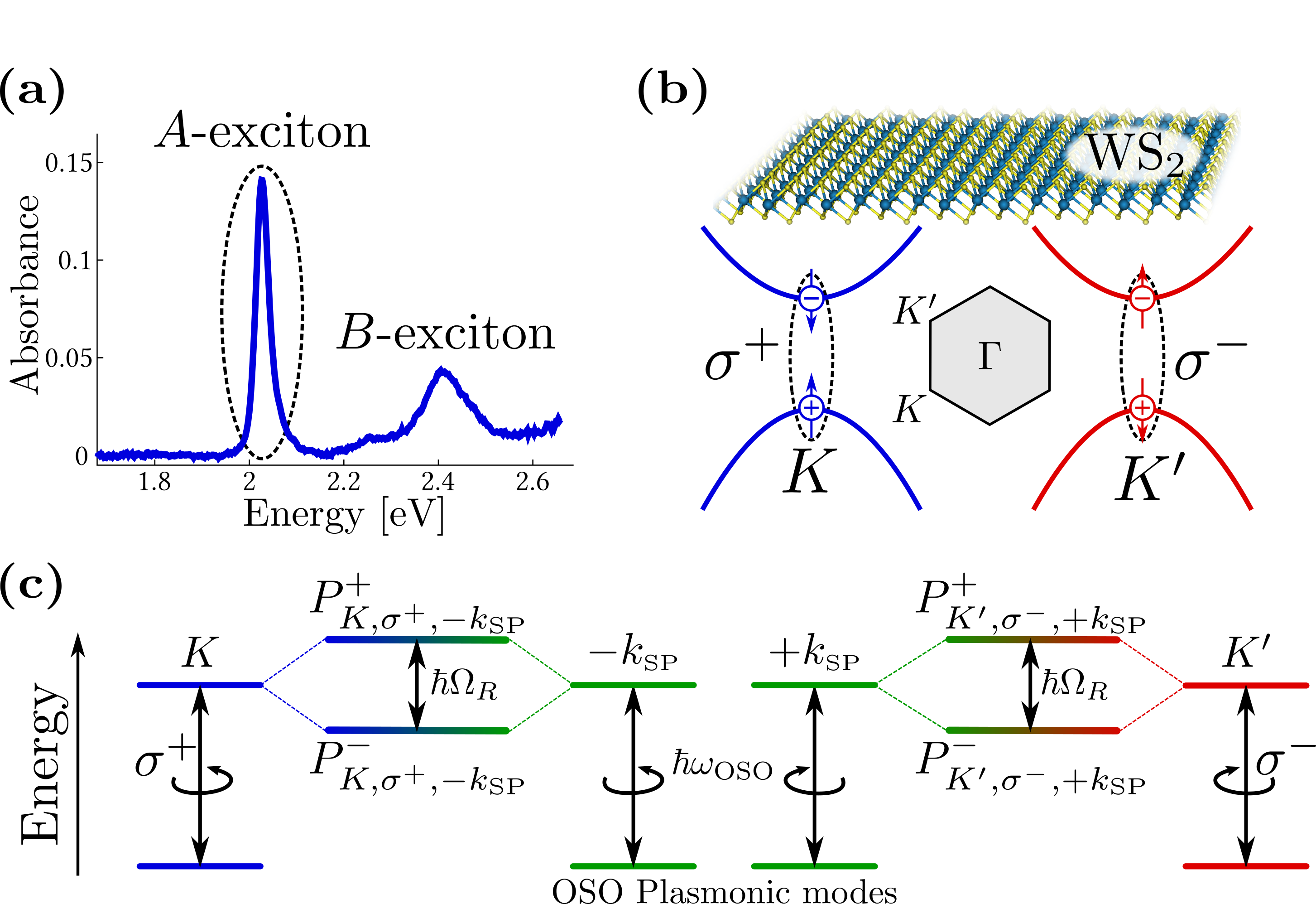
Figure 1: (a) Absorbance spectrum of a WS₂ monolayer as obtained from its transmission spectrum. (b) Crystal packing of a tungsten disulfide (WS₂) monolayer, and sketch of its electronic band structure around the points $K$ and $K^{\prime}$ of the Brillouin zone, with the corresponding optical selection rules for band-edge excitons formation under left ($\sigma^{+}$) and right ($\sigma^{-}$) circular excitation. (c) Energy level diagram of the $K$ and $K^{\prime}$ excitons of WS₂ strongly coupled to an OSO plasmonic mode at energy $\hbar\omega_{\rm OSO}$ and wavevector $\pm k_{\textrm{\tiny SP}}$.

Experimentally, our system, shown in Fig. 2(a), consists of a mechanically exfoliated monolayer of WS₂ covering a plasmonic OSO hole array, with a $5$ nm thick dielectric spacer (polymethyl methacrylate). The array, imaged in Fig. 2(b), is designed on a $(x,y)$ square lattice with a grating period $\Lambda$, and consists of rectangular nano-apertures $(160\times 90$ nm${}^{2})$ rotated stepwise along the $x$-axis by an angle $\phi=\pi/6$. The associated orbital period $6\times\Lambda$ sets a rotation vector $\bm{\Omega}=(\phi/\Lambda)\hat{z}$, which combines with the spin $\sigma$ of the incident light into a geometric phase $\Phi_{g}=-\Omega\sigma x$ Bliokh et al. (2008b). The gradient of this geometric phase imparts a momentum ${\bf k}_{g}=-\sigma(\phi/\Lambda)\hat{x}$ added to the matching condition on the array between the plasmonic ${\bf k}_{\rm SP}$ and incidence in-plane ${\bf k}_{\rm in}$ momenta: ${\bf k}_{\rm SP}={\bf k}_{\rm in}+(2\pi/\Lambda)(n\hat{x}+m\hat{y})+{\bf k}_{g}$. This condition defines different $(n,m)$ orders for the plasmonic dispersions, which are transverse magnetic (TM) and transverse electric (TE) polarized along the $x$ and $y$ axis of the array respectively (see Fig. 2(b)). The dispersive properties of such a resonator thus combines two modal responses: plasmon excitations directly determined on the square Bravais lattice of the grating for both $\sigma^{+}$ and $\sigma^{-}$ illuminations via $(2\pi/\Lambda)(n\hat{x}+m\hat{y})$, and spin-dependent plasmon OSO modes launched by the additional geometric momentum ${\bf k}_{g}$. It is important to note that the contribution of the geometric phase impacts the TM dispersions only. The period of our structure $\Lambda=480$ nm is optimized to have $n=+1$ and $n=-1$ TM modes resonant with the absorption energy of the $A$-exciton of WS₂ at $2.01$ eV for $\sigma^{+}$ and $\sigma^{-}$ illuminations respectively. This strict relation between $n=\pm 1$ and $\sigma=\pm 1$ is the OSO mechanism that breaks the left vs. right symmetry of the modal response of the array, which in this sense becomes chiral. Plasmon OSO modes are thus launched in counter-propagating directions along the $x$-axis for opposite spins $\sigma$ of the excitation light. In the case of a bare plasmonic OSO resonator, this is clearly observed in Fig. 2 (c). We stress that similar arrangements of anisotropic apertures have previously been demonstrated to allow for spin-dependent surface plasmon launching Shitrit et al. (2011); Huang et al. (2013); Lin et al. (2013); Jiang et al. (2016).

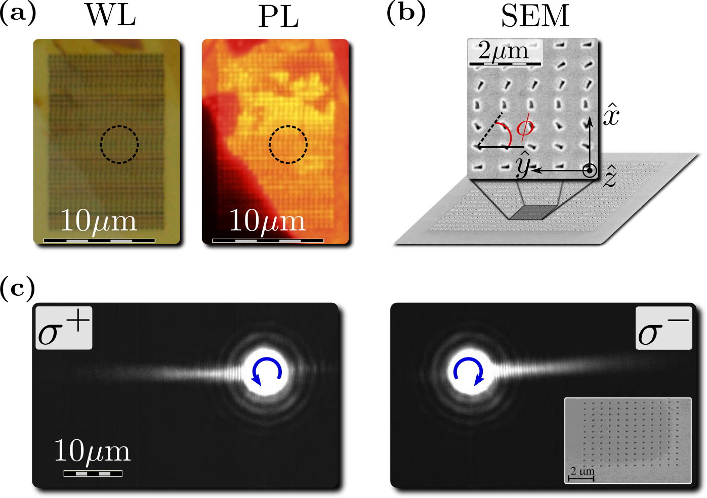
Figure 2: (a) White light (WL) microscope image of the sample and photoluminescence (PL) image of the same area under $2.58$ eV excitation. (b) SEM image of the plasmonic OSO resonator fabricated by sputtering $200$ nm of gold on a glass substrate coated by a $5$ nm thick chromium adhesion layer. The array with $\phi$-rotated rectangular apertures is milled through the metallic layers using a focused ion beam (FIB). (c) Real-space leakage radiation microscope Jiang et al. (2016) images of the surface plasmons launched by $\sigma^{+}$ and $\sigma^{-}$ excitations on a OSO plasmonic resonator similar to the one of panel (b).

As explained in the Supporting Information (Sec. A), the low transmission measured through our WS₂/plasmonic array sample (Fig. 2(a)) enables us to obtain absorption spectra directly from reflectivity spectra. Angle-resolved white light absorption spectra are hence recorded and shown in Fig. 3 (a) and (b) for left and right circular polarizations. In each case, two strongly dispersing branches are observed, corresponding to upper and lower chiralitonic states. As detailed in the Supporing Information (Sec. A), a fit of a coupled dissipative oscillator model to the dispersions enables us to extract a branch splitting $2\sqrt{\left(\hbar\Omega_{R}\right)^{2}-\left(\hbar\gamma_{\tiny\textrm{ex}}-\hbar\Gamma_{\tiny\textrm{OSO}}\right)^{2}}=40$ meV. With measured linewidths of the excitonic mode $\hbar\Gamma_{\tiny\textrm{OSO}}=80$ meV and of the plasmonic mode $\hbar\gamma_{\tiny\textrm{ex}}=26$ meV, this fitting yields a Rabi frequency of $\hbar\Omega_{\rm R}=70$ meV, close to our previous observations on non-OSO plasmonic resonators Wang et al. (2016a). We emphasize that this value clearly fulfills the strong coupling criterion with a figure-of-merit $\Omega_{\rm R}^{2}/(\gamma_{\rm exc}^{2}+\Gamma_{\rm OSO}^{2})=0.69$ larger than the $0.5$ threshold that must be reached for strong coupling Houdré (2005); Törmä and Barnes (2015). This demonstrates that our system does operate in the strong coupling regime, despite the relatively low level of visibility of the anti-crossing. This is only due $(i)$ to spatial and spectral disorders which leave, as always for collective systems, an inhomogeneous band of uncoupled states at the excitonic energy, and $(ii)$ to the fact that an uncoupled Bravais plasmonic branch is always superimposed to the plasmonic OSO mode, leading to asymmetric lineshapes clearly seen in Fig. 3 (a) and (b). As shown in the Supporting Information (Sec. A), the anti-crossing can actually be fully resolved through a first-derivative analysis of our absorption spectra.

In such strong coupling conditions, the two dispersion diagrams also show a clear mirror symmetry breaking with respect to the normal incident axis ($k_{x}=0$) for the two opposite optical spins. This clearly demonstrates the capability of our structure to act as a spin-momentum locked polariton launcher. From the extracted linewidth that gives the lifetime of the chiralitonic mode and the curvature of the dispersion relation that provides its group velocity, we can estimate a chiraliton propagation length of the order of $4~{}\mu$m, in good agreement with the measured PL diffusion length presented in the Supporting Information (Sec. B).

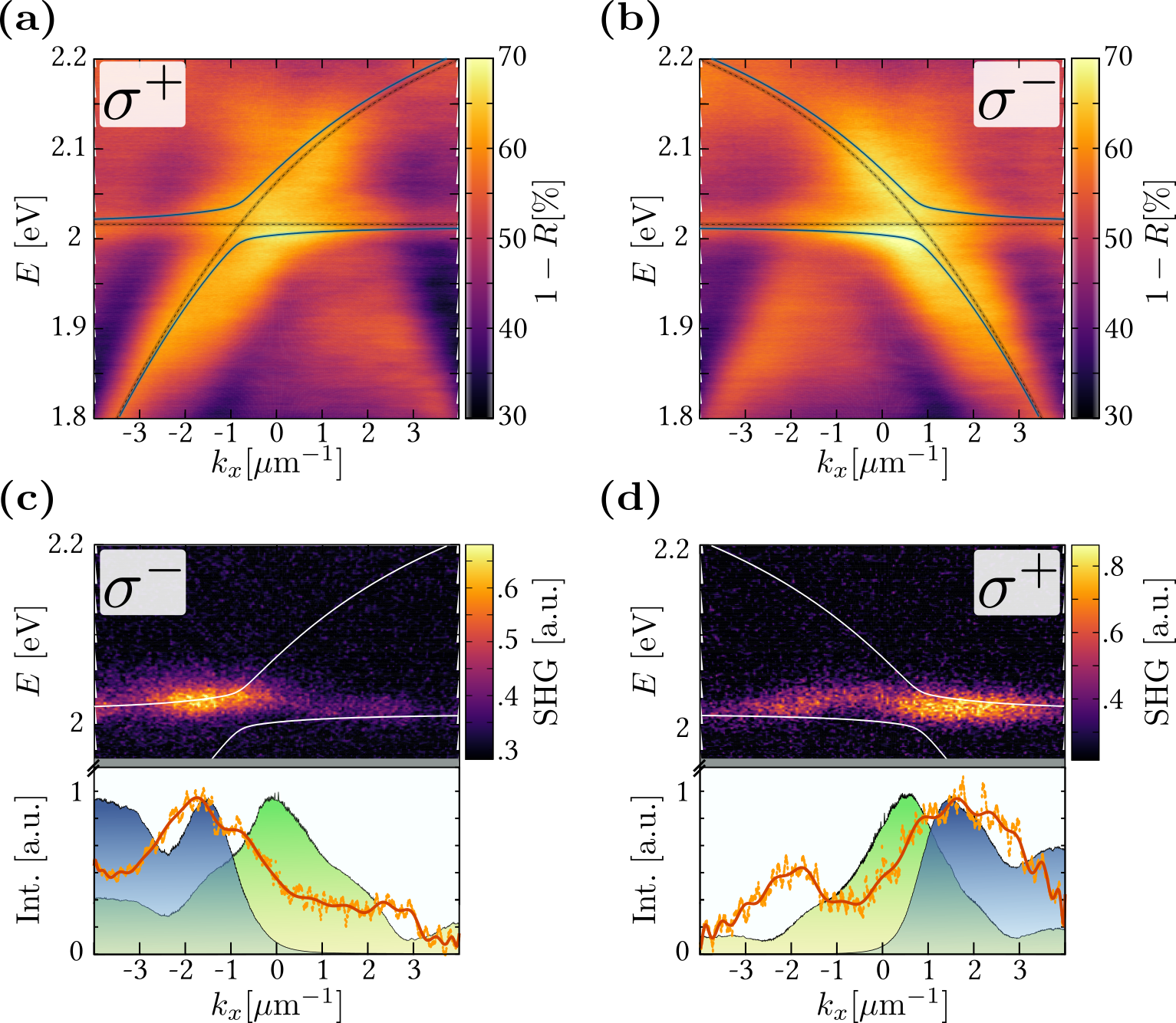
Figure 3: Angle-resolved absorption spectrum of the sample analyzed in (a) left and (b) right circular polarizations, with the best fit coupled oscillator model drawn. Angle-resolved resonant second harmonic spectrum for (c) right and (d) left circular excitations at $1.01$eV. Corresponding crosscuts are displayed with the angular profile of the SH signal (red curves), of the absorption spectra at $2$ eV (green shades) and of the product (blue shades) between the absorption and the $4^{\rm th}$ power of the excitonic Hopfield coefficient of the chiralitonic state -see details in the Supporting Information (Sec. D) .

In view of chiral light-chiral matter interactions, we further investigate the interplay between this plasmonic chirality and the valley-contrasting chirality of the WS₂ monolayer. A first demonstration of such an interplay is found in the resonant second harmonic (SH) response of the strongly coupled system. Indeed, monolayer TMDs have been shown to give a high valley contrast in the generation of a SH signal resonant with their $A$-excitons Seyler et al. (2015). As we show in Supporting Information (Sec. G) such high SH valley contrast are measured on a bare WS₂ monolayer. The optical selection rules for SH generation are opposite to those in linear absorption since the process involves two excitation photons, and are more robust since the SH process is instantaneous.

The angle resolved resonant SH signals are shown in Fig. 3 (c) and (d) for right and left circularly polarized excitation. The SH signals are angularly exchanged when the spin of the excitation is reversed with a right vs. left contrast (ca. $20\%$) close to the one measured on the reflectivity maps (ca. $15\%$). This unambigously demonstrates the selective coupling of excitons in one valley to surface plasmons propagating in one direction, thus realizing valley-contrasting chiralitonic states with spins locked to their propagation wavevectors:

$$|P^{\pm}_{K,\sigma^{+},-k_{\textrm{\tiny SP}}}>=|g_{K},1_{\sigma^{+}},-k_{\textrm{\tiny SP}}>\pm|e_{K},0_{\sigma^{+}},-k_{\textrm{\tiny SP}}>$$

$$|P^{\pm}_{K^{\prime},\sigma^{-},+k_{\textrm{\tiny SP}}}>=|g_{K^{\prime}},1_{\sigma^{-}},+k_{\textrm{\tiny SP}}>\pm|e_{K^{\prime}},0_{\sigma^{-}},+k_{\textrm{\tiny SP}}>,$$

where $e_{i}(g_{i})$ corresponds to the presence (absence) of an exciton in the valley $i=(K,K^{\prime})$ of WS₂, and $1_{j}(0_{j})$ to 1 $(0)$ plasmon in the mode of polarization $j=(\sigma^{+},\sigma^{-})$ and wavevector $\pm k_{\textrm{\tiny SP}}$.

The detailed features of SH signal (crosscuts in Fig. 3 (c) and (c)) reveal within the bandwidth of our pumping laser the contributions of both the uncoupled excitons and the upper chiraliton to the SH enhancement. The key observation, discussed in the Supporting Information (Sec. D), is the angular dependence of the main SH contribution. This contribution, shifted from the anticrossing region, is a feature that gives an additional proof of the strongly coupled nature of our system because it is determined by the excitonic Hopfield coefficient of the spin-locked chiralitonic state. In contrast, the residual SH signal related to the uncoupled (or weakly coupled) excitons simply follows the angular profile of the absorption spectra taken at $2$ eV, thus observed over the anticrossing region. Resonant SH spectroscopy of our system therefore confirms the presence of the chiralitonic states, with the valley contrast of WS₂ and the spin-locking property of the OSO plasmonic resonator being imprinted on these new eigenstates of the system.

Revealed by these resonant SH measurements, the spin-locking property of chiralitonic states incurs however different relaxation mechanisms through the dynamical evolution of the chiralitons. In particular, excitonic intervalley scattering can erase valley contrast in WS₂ at RT Hanbicki et al. (2016) -see below. In our configuration, this would transfer chiraliton population from one valley to the other, generating via optical spin-locking, a reverse flow, racemizing the chiraliton population. This picture however does not account for the possibility of more robust valley contrasts in strong coupling conditions, as recently reported with MoSe₂ in Fabry-Pérot cavities Dufferwiel et al. (2017). The chiralitonic flow is measured by performing angle resolved polarized PL experiments, averaging the signal over the PL lifetime of ca. $200$ ps (see Supporting Information, Sec. D and E). For these experiments, the laser excitation energy is chosen at $1.96$ eV, slightly below the WS₂ band-gap. At this energy, the measured PL results from a phonon-induced up-convertion process that minimizes intervalley scattering events Jones et al. (2016). The difference between PL dispersions obtained with left and right circularly polarized excitations is displayed in Fig. 4 (a), showing net flows of chiralitons with spin-determined momenta. This is in agreement with the differential white-light reflectivity map $R_{\sigma^{-}}-R_{\sigma^{+}}$ of Fig. 4 (b). Considering that this map gives the sorting efficiency of our OSO resonator, such correlations in the PL implies that the effect of the initial spin-momentum determination of the chiralitons (see Fig. 3 (e) and (f)) is still observed after $200$ ps at RT. After this PL lifetime, a net chiral flow $\mathcal{F}=I_{\sigma^{-}}-I_{\sigma^{+}}$ of $\sim 6\%$ is extracted from Fig. 4 (a). This is the signature of a chiralitonic valley polarization, in striking contrast with the absence of valley polarization that we report for a bare WS₂ monolayer at RT in the Supporting Information, Sec. G. The extracted net flow is however limited by the finite optical contrast $\mathcal{C}$ of our OSO resonator, which we measure at a $15\%$ level from a cross-cut taken on Fig. 4 (b) at $1.98$ eV. It is therefore possible to infer that a chiralitonic valley contrast of $\mathcal{F}/\mathcal{C}\simeq 40\%$ can be reached at RT for the strongly coupled WS₂ monolayer. As mentioned above, we understand this surprisingly robust contrast by invoking the fact that under strong coupling conditions, valley relaxation is outweighted by the faster Rabi energy exchange between the exciton of each valley and the corresponding plasmonic OSO mode, as described in the Supporting Information (Sec. A). From the polaritonic point of view, the local dephasing and scattering processes at play on bare excitons -that erase valley contrasts on a bare WS2 flake as observed in the Supporting Information (Sec. G)- are reduced by the delocalized nature of the chiralitonic state, a process akin to motional narrowing and recently observed on other polaritonic systems Whittaker et al. (1996); Dufferwiel et al. (2017); Chen et al. (2017); Kleemann et al. (2017).

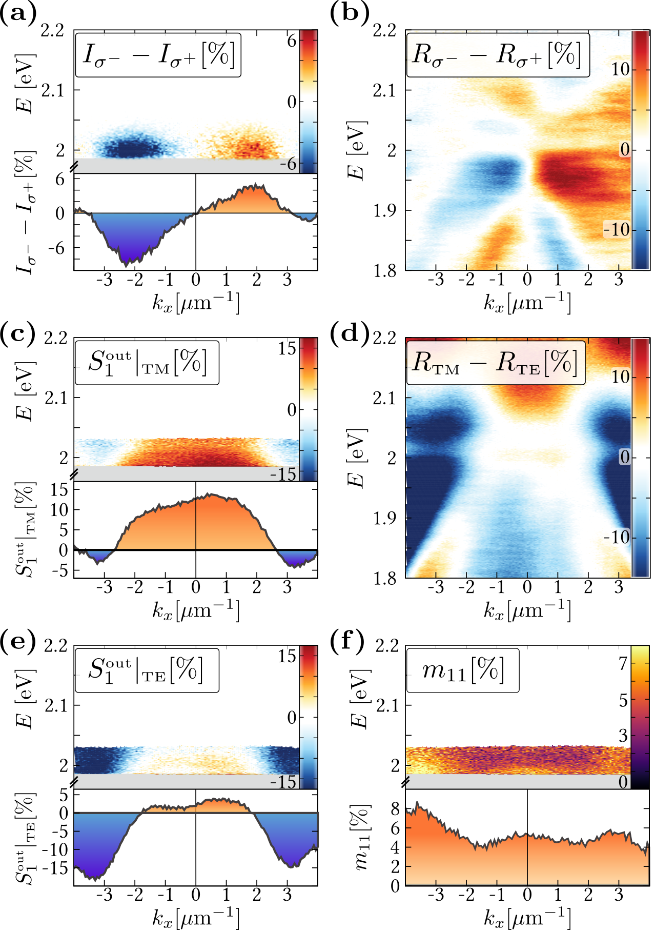
Figure 4: (a) Differential PL dispersion spectrum for left and right circularly polarized excitations. The shaded regions in all panels are removed by the laser line filter, and the cross-cuts are taken at $2$ eV. (b) Differential angle-resolved reflection spectrum for left and right circularly polarized light. (c), (e) Angle-resolved spectrum of the normalized coefficient $S_{1}^{\textrm{\tiny out}}|_{\textrm{\tiny TM(TE)}}/S_{0}$ of the PL Stokes vector for a TM(TE) polarized excitation (see text for details). Note that we have put a detection threshold below $100$ photon counts that cuts the signal above $\sim 2.03$ eV in panels (a), (c), (e) and (f). (d) Differential angle-resolved reflection spectrum obtained from analyzed TM and TE measurements. (f) $k_{x}$-energy dispersion of the degree of chiralitonic inter-valley coherence $m_{11}$ computed from (c) and (e).

As a consequence of this motional narrowing effect, such a strongly coupled system involving atomically thin crystals of TMDs could then provide new ways to incorporate intervalley coherent dynamics Jones et al. (2013); Hao et al. (2016); Wang et al. (2016b); Schmidt et al. (2016); Ye et al. (2017) into the realm of polariton physics. To illustrate this, we now show that two counter-propagating flows of chiralitons can evolve coherently. It is clear from Fig. 1 (c) that within such a coherent superposition of counter-propagating chiralitons

$$|\Psi>=|P^{\pm}_{K,\sigma^{+},-k_{\textrm{\tiny SP}}}>+|P^{\pm}_{K^{\prime},\sigma^{-},+k_{\textrm{\tiny SP}}}>$$ (1)

flow directions and spin polarizations become non-separable. Intervalley coherence is expected to result in a non-zero degree of linearly polarized PL when excited by the same linear polarization. This can be monitored by measuring the $S_{1}=I_{\textrm{\tiny TM}}-I_{\textrm{\tiny TE}}$ coefficient of the PL Stokes vector, where $I_{\textrm{\tiny TM}(\textrm{\tiny TE})}$ is the emitted PL intensity analyzed in TM (TE) polarization. This coefficient is displayed in the $k_{x}$-energy plane in Fig. 4(c) for an incident TM polarized excitation at $1.96$ eV. Fig. 4(e) displays the same coefficient under TE excitation. A clear polarization anisotropy on the chiraliton emission is observed for both TM and TE excitation polarizations, both featuring the same symmetry along the $k_{x}=0$ axis as the differential reflectivity dispersion map $R_{\textrm{\tiny TM}}-R_{\textrm{\tiny TE}}$ shown in Fig. 4(d). As detailed in the Supporting Information (Sec. F), the degree of chiralitonic intervalley coherence can be directly quantified by the difference $(S_{1}^{\textrm{\tiny out}}|_{\textrm{\tiny TM}}-S_{1}^{\textrm{\tiny out}}|_{\textrm{\tiny TE}})/2$, which measures the PL linear depolarization factor displayed (as $m_{11}$) in Fig. 4 (f). By this procedure, we retrieve a chiralitonic intervalley coherence that varies between $5\%$ and $8\%$ depending on $k_{x}$. Interestingly, these values that we reach at RT have magnitudes comparable to those reported on a bare WS₂ monolayer at 10 K Zhu et al. (2014). This unambiguously shows how such strongly coupled TMD systems can sustain RT coherent dynamics robust enough to be observed despite the long exciton PL lifetimes and plasmonic propagation distances.

In summary, we demonstrate valley contrasting spin-momentum locked chiralitonic states in an atomically thin TMD semiconductor strongly coupled to a plasmonic OSO resonator. Likely, the observation of such contrasts even after 200 ps lifetimes is made possible by the unexpectedly robust RT coherences inherent to the strong coupling regime. Exploiting such robust coherences, we measure chiralitonic flows that can evolve in superpositions over micron scale distances. Our results show that the combination of OSO interactions with TMD valleytronics is an interesting path to follow in order to explore and manipulate RT coherences in chiral quantum architectures Coles et al. (2016); Low et al. (2017).

Author Contributions - T. C. and S. A. contributed equally to this work.

I Supporting Information

II A: Linear absorption dispersion analysis

Angle resolved absorption spectra are given from the measured reflectivity of the WS₂ flake on top of the plasmonic grating $R_{\tiny\textrm{sample}}$ with:

$$A=1-R_{\tiny\textrm{sample}}/R_{\tiny\textrm{substrate}},$$ (2)

where $R_{\tiny\textrm{substrate}}$ is the angle resolved reflectivity of the optically thick (200 nm thickness) Au substrate. The $1\%$ max. transmission through the structure can be safely neglected. As we explain in the main text, the resulting dispersion spectra are broadened by the contribution of different plasmonic modes as well as coupled and uncoupled exciton populations.

In order to highlight the polaritonic contribution in the absorption spectra, we calculate the first derivative of the reflectivity dispersions $\textrm{d}\left[R_{\tiny\textrm{sample}}/R_{\tiny\textrm{substrate}}\right]/\textrm{d}E$. The derivative was approximated by interpolating the reflectivity spectra on an equally spaced wavelength grid of step $\Delta\lambda=0.55$ nm and using the following finite difference expression valid up to fourth order in the grid step:

$$\frac{\textrm{d}R}{\textrm{d}\lambda}(\lambda_{0})\simeq\frac{\frac{1}{12}R(\lambda_{-2})-\frac{2}{3}R(\lambda_{-1})+\frac{2}{3}R(\lambda_{+1})-\frac{1}{12}R(\lambda_{+2})}{\Delta\lambda},$$ (3)

where $R(\lambda_{n})$ is the reflectivity evaluated $n$ steps away from $\lambda_{0}$. The resulting first derivative reflectivity spectra were then converted to an energy scale and plotted as dispersion diagrams in Fig. 5 (a) and (b).

In these first derivative reflectivity maps, the zero-crossing points correspond to the peak positions of the modes, and the maxima and minima indicate the inflection points of the reflectivity lineshapes. At the excitonic asymptotes of the dispersion curves, where the polaritonic linewidth is expected to match that of the bare WS₂ exciton, we read a linewidth of $26$ meV from the maximum to minimum energy difference of the derivative reflectivity maps. This value is equal to the full width at half maximum (FWHM) $\hbar\gamma_{\rm exc}$ that we measured from the absorption spectrum of a bare WS₂ flake on a dielectric substrate.

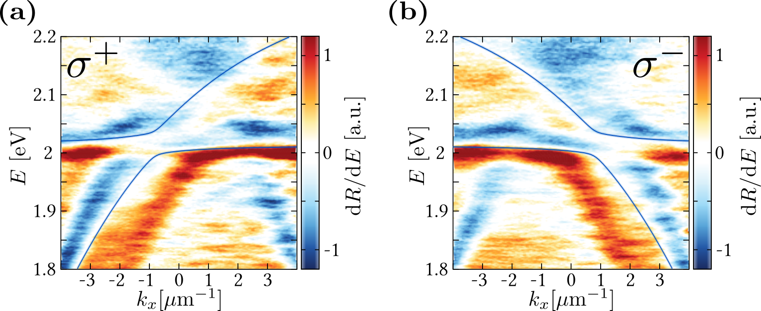
Figure 5: First derivative reflectivity maps in (a) left and (b) right circular polarizations, with the best fit coupled oscillator model drawn.

On the low energy plasmonic asymptotes, we clearly observe the effect of the Bravais and OSO modes, partially overlapping in an asymmetric broadening of the branches. In this situation, a measure of the mode half-widths can be extracted from the (full) widths of the positive or negative regions of the first differential reflectivity maps. This procedure yields an energy half-width for the plasmonic modes of $\hbar\Gamma_{\rm OSO}/2=40$ meV. This width in energy can be related to an in-plane momentum width of ca. $0.5~{}\mu\textrm{m}^{-1}$ via the plasmonic group velocity $v_{G}=\partial E/\partial k=87$ meV$\cdot\mu$m, that we calculate from the branch curvature at $1.85$ eV. This in-plane momentum width results in a plasmonic propagation length of about $4~{}\mu$m. This value is in very good agreement with the measured PL extension above the structure, as discussed in section B below, validating our estimation of the mode linewidth $\hbar\Gamma_{\rm OSO}=80$ meV.

The dispersive modes of the system can be modeled by a dipolar Hamiltonian, where excitons in each valley are selectively coupled to degenerated OSO plasmonic modes of opposite wavevectors $\pm{\bf k}_{\rm SP}$, as depicted in Fig. 2 in the main text:

$$\mathcal{H}=\sum_{k_{x}}\left[\mathcal{H}_{\tiny\textrm{OSO}}(k_{x})+\mathcal{H}_{\tiny\textrm{ex}}+\mathcal{H}_{\tiny\textrm{int}}(k_{x})\right],$$ (4)

which consists of three different contributions:

$$\mathcal{H}_{\tiny\textrm{OSO}}(k_{x})=\hbar\omega_{\tiny\textrm{OSO}}(k_{x})\left(a^{\dagger}_{k_{x}}a_{k_{x}}+a^{\dagger}_{-k_{x}}a_{-k_{x}}\right),$$ (5)

$$\mathcal{H}_{\tiny\textrm{ex}}(k_{x})=\hbar\omega_{\tiny\textrm{ex}}\left(b^{\dagger}_{K-k_{x}}b_{K-k_{x}}+b^{\dagger}_{K^{\prime}+k_{x}}b_{K^{\prime}+k_{x}}\right),$$ (6)

$$\mathcal{H}_{\tiny\textrm{int}}(k_{x}) = \hbar g\left(a^{\dagger}_{k_{x}}+a_{k_{x}}\right)\left(b^{\dagger}_{K^{\prime}+k_{x}}+b_{K^{\prime}+k_{x}}\right)$$ (7)

$$+\hbar g\left(a^{\dagger}_{-k_{x}}+a_{-k_{x}}\right)\left(b^{\dagger}_{K-k_{x}}+b_{K-k_{x}}\right),$$

where $a(a^{\dagger})$ are the lowering (raising) operators of the OSO plasmonic modes of energy $\hbar\omega_{\tiny\textrm{OSO}}(k_{x})$, $b(b^{\dagger})$ are the lowering (raising) operators of the exciton fields of energy $\hbar\omega_{\tiny\textrm{ex}}$, and $g=\Omega_{R}/2$ is the light-matter coupling frequency. In this hamiltonian the chiral light-chiral matter interaction is effectively accounted for by coupling excitons of the valley $K^{\prime}(K)$ to plasmons propagating with wavevectors $k_{x}(-k_{x})$. Moreover, the dispersion of the exciton energy can be neglected on the scale of the plasmonic wavevector ${\bf k}_{\rm SP}$.

Using the Hopfield procedure Ciuti et al. (2005), we can diagonalize the total Hamiltonian by finding polaritonic normal mode operators $P^{\pm}_{K(K^{\prime})}$ associated with each valley, and obeying the following equation of motion at each $k_{x}$

$$\left[P^{\pm}_{K(K^{\prime})},\mathcal{H}\right]=\hbar\omega_{\pm}P^{\pm}_{K(K^{\prime})},$$ (8)

with $\omega_{\pm}>0$. In the rotating wave approximation (RWA), justified here by the moderate coupling strength (see below), $P^{j}_{\lambda}\simeq\alpha^{j}_{\lambda}a+\beta^{j}_{\lambda}b$, $j\in\{+,-\}$ and $\lambda\in\{K,K^{\prime}\}$. The plasmonic and excitonic Hopfield coefficients $\alpha^{j}_{\lambda}(k_{x})$ and $\beta^{j}_{\lambda}(k_{x})$ are obtained by diagonalizing the following matrix for every $k_{x}$

$$\left(\begin{array}[]{cccc}\hbar\omega_{\tiny\textrm{OSO}}&i\hbar\Omega_{\rm R}&0&0\\ -i\hbar\Omega_{\rm R}&\hbar\omega_{\tiny\textrm{ex}}&0&0\\ 0&0&-\hbar\omega_{\tiny\textrm{OSO}}&i\hbar\Omega_{\rm R}\\ 0&0&-i\hbar\Omega_{\rm R}&-\hbar\omega_{\tiny\textrm{ex}}\end{array}\right).$$ (9)

The dynamics of the coupled system will be ruled by the competition between the coherent evolution described by the Hamiltonian (4) and the different dissipative processes contributing to the uncoupled modes linewidths. This can be taken into account by including the measured linewidths as imaginary parts in the excitonic and plasmonic mode energies (Weisskopf-Wigner approach). Under such conditions, we evaluate the eigenvalues $\omega_{\pm}$ of the the matrix (9). The real parts of $\omega_{\pm}$ are then fitted to the maxima of the angle resolved reflectivity maps presented on Fig. 3 in the main text, or to the zeros of the first derivative reflectivity maps shown here in Fig. 5 (a) and (b). Both procedures give the same best fit that yields the polaritonic branch splitting as Houdré (2005); Törmä and Barnes (2015)

$$\hbar(\omega_{+}-\omega_{-})=2\sqrt{\left(\hbar\Omega_{R}\right)^{2}-\left(\hbar\gamma_{\tiny\textrm{ex}}-\hbar\Gamma_{\tiny\textrm{OSO}}\right)^{2}}$$ (10)

which equals $40$ meV. From the determination (see above) of the FWHM of the excitonic $\hbar\gamma_{\tiny\textrm{ex}}$ and plasmonic $\hbar\Gamma_{\tiny\textrm{OSO}}$ modes, we evaluate a Rabi energy $\hbar\Omega_{R}=70$ meV.

These values give a ratio

$$\left(\hbar\Omega_{R}\right)^{2}/\left(\left(\hbar\gamma_{\tiny\textrm{ex}}\right)^{2}+\left(\hbar\Gamma_{\tiny\textrm{OSO}}\right)^{2}\right)=0.69,$$ (11)

above the $0.5$ threshold which is the strong coupling criterion -see Houdré (2005) for a detailed discussion. This figure-of-merit of $0.69>0.5$ therefore clearly demonstrates that our system is operating in the strong coupling regime.

Interestingly, the intervalley scattering rate $\hbar\gamma_{KK^{\prime}}$ does not enter in this strong coupling criterion. Indeed, such events corresponding to an inversion of the valley indices $K\leftrightarrow K^{\prime}$ do not contribute to the measured excitonic linewidth, and are thus not detrimental to the observation of strong coupling. In the $\hbar\Omega_{R}\ll\hbar\gamma_{KK^{\prime}}$ limit, the Hamiltonian (4) would reduce to the usual RWA Hamiltonian and the valley contrasting chiralitonic behavior would be lost. The results gathered in Fig. 4 in the main text clearly show that this is not the case for our system, allowing us to conclude that the Rabi frequency overcomes such intervalley relaxation rates. Remarkably, strong coupling thus allows us to put an upper bounds to those rates, in close relation with Holmes and Forrest (2004).

III B: Chiraliton diffusion length

The diffusion length of chiralitons can be estimated by measuring the extent of their photoluminescence (PL) under a tightly focused excitation. To measure this extent, we excite a part of a WS₂ monolayer located above the plasmonic hole array (Fig. S5(a) and (b)). This measurement is done on a home-built PL microscope, using a $100\times$ microscope objective of 0.9 numerical aperture and exciting the PL with a HeNe laser at $1.96$ eV, slightly below the exciton band-gap. A diffraction-limited spot of $430$ nm half-width is obtained (Fig. S5(c)) by bringing the sample in the focal plane of the microscope while imaging the laser beam on a cooled CCD camera. The PL is collected by exciting at $10~{}\mu$W of optical power, and is filtered from the scattered laser light by a high-energy-pass filter. The resulting PL image is shown in Fig. S5(d), clearly demonstrating the propagating character of the emitting chiralitons. The logarithmic cross-cuts (red curves in (c) and (d)) reveal a propagation length of several microns.

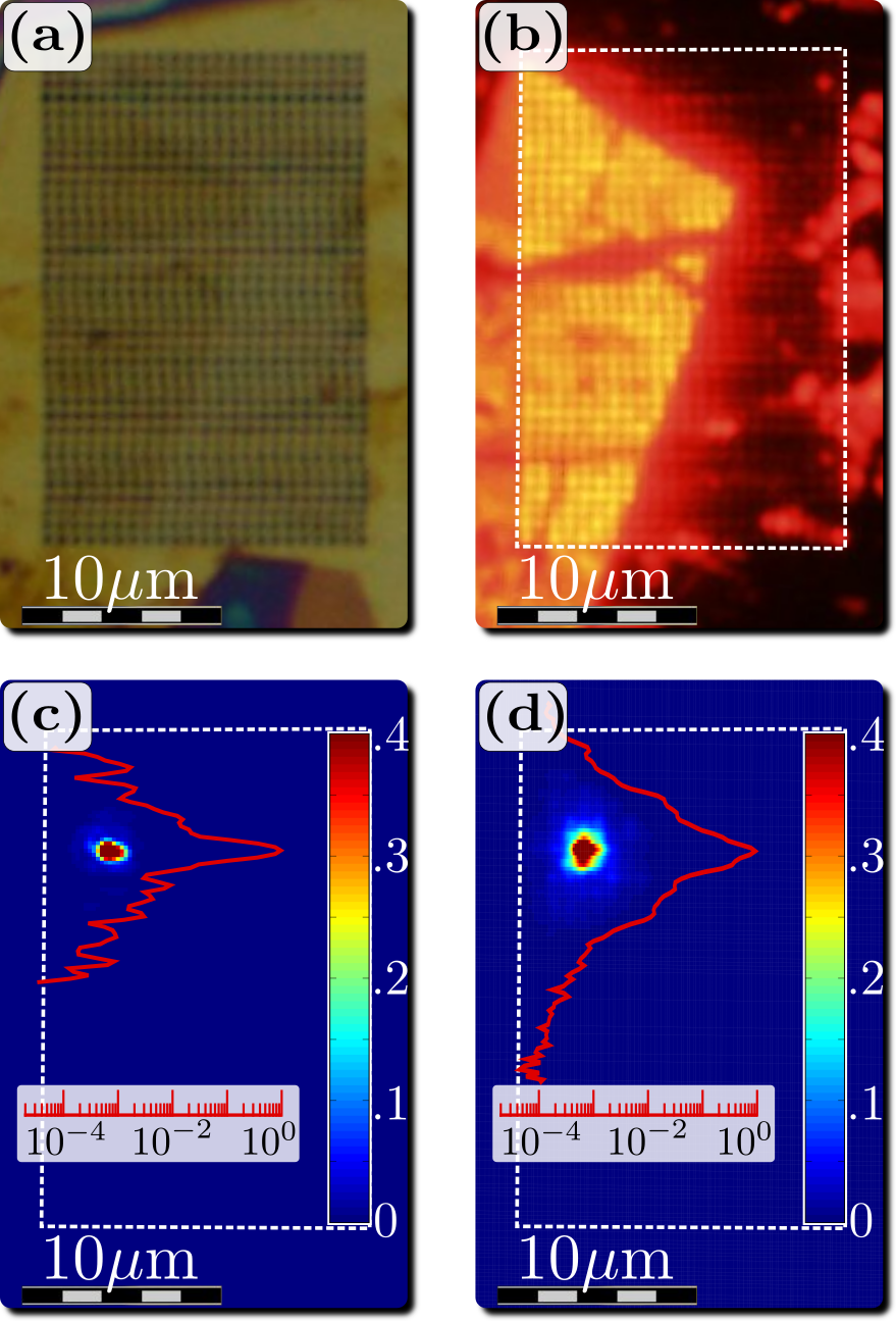
Figure 6: (a) White light image of a WS₂ flake covering the plasmonic hole array, and (b) its wide field PL. (c) Normalized image of the diffraction-limited laser spot on the structure (indicated by the white dashed rectangle in (c) and (d)). The logarithmic scale cross-cuts (red curves in (c) and (d)) are taken along the vertical axis, through the intensity maximum. (d) Normalized chiraliton PL image.

We note that the PL of the WS₂ monolayer also extends further away from the flake above the OSO array (Fig. S6(b)). We extract from this result the $1/e$ decay length of the plasmon to be $\sim 3.4~{}\mu$m. This value nicely agrees with that obtained in section A from the linear dispersion analysis.

IV C: Resonant Second Harmonic generation on a WS₂ monolayer

As discussed in the main text, TMD monolayers have recently been shown to give a high valley contrast in the generation of a second harmonic (SH) signal resonant with their $A$-excitons. We obain a similar result when measuring a part of the WS₂ monolayer sitting above the bare metallic surface, i.e. aside from the plasmonic hole array. In Fig. S7 we show the SH signal obtained in left and right circular polarization for an incident femto-second pump beam (120 fs pulse duration, 1 kHz repetition rate at 1.01 eV) in (a) left and (b) right circular polarization. This result confirms that the SH signal polarization is a good observable of the valley degree of freedom of the WS₂ monolayer, with a contrast reaching ca. $80\%$. In Fig. 3 (c) and (d) in the main text, we show how this valley contrast is imprinted on the chiralitonic states.

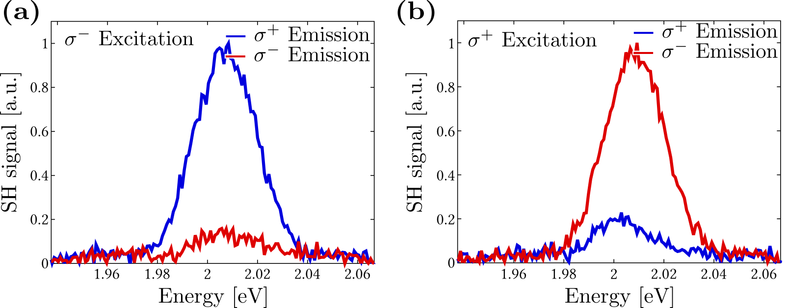
Figure 7: Resonant SH spectrum for left and right circular analysis, for (a) left and (b) right circular excitation at $1.01$eV.

V D: Resonant SH generation in the strong coupling regime

The resonant SH signal writes as Heinz et al. (1982); Chervy et al. (2016):

$$I(2\omega)\propto(\rho_{\omega}I_{\omega})^{2}\cdot|\chi^{(2)}(2\omega)|^{2}\cdot\rho_{2\omega}$$ (12)

where $I_{\omega}$ is the pump intensity, $\chi^{(2)}(2\omega)$ the second order susceptibility, $\rho_{\omega}$ the optical mode density of the resonator related to the fraction of the pump intensity that reaches WS₂ and $\rho_{2\omega}$ the optical mode density of the resonator that determines the fraction of SH intensity decoupled into the far field. While $\rho_{\omega}$ can safely be assumed to be non-dispersive at $\hbar\omega=1$ eV, the dispersive nature of the resonator leads to $\rho_{2\omega}$ strongly dependent on the in-plane wave vector $k_{x}$. The optical mode density being proportional to the absorption, $\rho_{2\omega}(k_{x})$ is given by the angular absorption spectrum crosscut at $2\hbar\omega=2$ eV, displayed in the lower panels of Fig. 3 (e) and (f) in the main text.

Under the same approximations of Lin et al. (1993), the resonant second order susceptibility can be written as

$$\chi^{(2)}(2\omega)=\alpha^{(1)}(2\omega)\sum_{n}\frac{K_{eng}}{\omega_{ng}-\omega}$$ (13)

where $\sum_{n}$ sums over virtual electronic transitions, and $K_{eng}=\langle e|{\bf p}|g\rangle\otimes\langle e|{\bf p}|n\rangle\otimes\langle n|{\bf p}|g\rangle$ is a third-rank tensor built on the electronic dipole moments ${\bf p}$ taken between the $e,n,g$ states. The prefactor $\alpha^{(1)}(2\omega)$ is the linear polarizability of the system at frequency $2\omega$, yielding resonantly enhanced SH signal at every allowed $|g\rangle\rightarrow|e\rangle$ electronic transitions of the system.

With two populations of uncoupled and strongly coupled WS₂ excitons, the SH signal is therefore expected to be resonantly enhanced when the SH frequency matches the transition frequency of either uncoupled or strongly coupled excitons. When the excited state is an uncoupled exciton associated with a transition energy fixed at frequency $2\hbar\omega=2$ eV for all angles, the tensor $K_{eng}$ is non-dispersive and the SH signal is simply determined and angularly distributed from $\rho_{2\omega}(k_{x})$.

When the excited state is a strongly coupled exciton, the resonant second order susceptibility becomes dispersive with $\chi^{(2)}(2\omega,k_{x})$. This is due to the fact that the tensor $K_{eng}$ incorporates the excitonic Hopfield coefficient of the polaritonic state involved in the electronic transition $|g\rangle\rightarrow|e\rangle$ when the excited state is a polaritonic state. In our experimental conditions with a pump frequency at $1$ eV, this excited state is the upper polaritonic state with $|e\rangle\equiv|P^{+}_{K(K^{\prime}),\sigma^{\pm}},\mp k_{\rm SP}\rangle$ and therefore $K_{eng}\propto[\beta_{K(K^{\prime})}^{+}(k_{x})]^{2}$. This dispersive excitonic Hopfield coefficient is evaluated by the procedure described in details above, Sec. A. The profile of the SH signal then follows the product between the optical mode density $\rho_{2\omega}(k_{x})$ and $|\chi^{(2)}(2\omega,k_{x})|^{2}\propto[\beta_{K(K^{\prime})}^{+}(k_{x})]^{4}$.

These two contributions are perfectly resolved in the SH data displayed in Fig. 3 (e) and (f) in the main text. The angular distribution of the main SH signal clearly departs from $\rho_{2\omega}(k_{x})$, revealing the dispersive influence of $\beta_{K(K^{\prime})}^{+}(k_{x})$. This is perfectly seen on the crosscuts displayed in the lower panels of Figs. 3 (e) and (f) in the main text. This feature is thus an indisputable proof of the existence of chiralitonic states, i.e. of the strongly coupled nature of our system.

A residual SH signal is also measured which corresponds to the contribution of uncoupled excitons. This residual signal is measured in particular within the anticrossing region, as expected from the angular profile of $\rho_{2\omega}(k_{x})$ shown in the lower panels of Figs. 3 (e) and (f) in the main text.

Finally, the angular features of the SH signal exchanged when the spin of the pump laser is flipped from $\sigma^{+}$ to $\sigma^{-}$ reveal how valley contrasts have been transferred to the polariton states. These features therefore demonstrate the chiral nature of the strong coupling regime, i.e. the existence of genuine chiralitons.

VI E: PL lifetime measurement on the strongly coupled system

The PL lifetime of the strongly coupled system is measured by time-correlated single photon counting (TCSPC) under pico-second pulsed excitation (instrument response time $120$ ps, 20 MHz repetition rate at 1.94 eV). The arrival time histogram of PL photons, when measuring a part of the WS₂ monolayer located above the plasmonic hole array, gives the decay dynamic shown in Fig. S8(a). On this figure we also display the PL decay of a reference WS₂ monolayer exfoliated on a dielectric substrate (polydimethylsiloxane), as well as the instrument response function (IRF) measured by recording the excitation pulse photons scattered by a gold film. Following the procedure detailed in Federspiel et al. (2015), we define the calculated decay times $\tau_{\textrm{\tiny calc}}$ as the area under the decay curves (corrected for their backgrounds) divided by their peak values. This yields a calculated IRF time constant $\tau_{\textrm{\tiny calc}}^{\textrm{\tiny IRF}}=157$ ps, and calculated PL decay constants $\tau_{\textrm{\tiny calc}}^{\textrm{\tiny ref}}=1.39$ ns and $\tau_{\textrm{\tiny calc}}^{\textrm{\tiny sample}}=384$ ps for the reference bare flake and the strongly coupled sample respectively. The real decay time constants $\tau_{\textrm{\tiny real}}$ corresponding to the calculated ones can then be estimated by convoluting different monoexponential decays with the measured IRF, computing the corresponding $\tau_{\textrm{\tiny calc}}$ and interpolating this calibration curve (Fig. S7(b)) for the values of $\tau_{\textrm{\tiny calc}}^{\textrm{\tiny ref}}$ and $\tau_{\textrm{\tiny calc}}^{\textrm{\tiny sample}}$. This results in $\tau_{\textrm{\tiny real}}^{\textrm{\tiny ref}}=1.06$ ns and $\tau_{\textrm{\tiny real}}^{\textrm{\tiny sample}}=192$ ps.

While the long life-time (ns) of the bare WS₂ exciton has been attributed to the trapping of the exciton outside the light-cone at RT through phonon scattering Pöllmann et al. (2015); Robert et al. (2016), Fig. S8 simply shows that the exciton life time is reduced by the presence of the metal or the OSO resonator. Clearly, the competition induced under strong coupling conditions between the intra and inter valley relaxation rates and the Rabi oscillations must act under shorter time scales that are not resolved here.

Figure 8: (a) TCSPC histogram showing the PL decay dynamic of the strongly coupled WS₂ monolayer (red curve), as compared to that of a bare WS₂ monolayer on a dielectric substrate (green curve). The IRF of our measurement apparatus is shown in blue. (b) Calibration (blue curve) used to retrieve $\tau_{\textrm{\tiny real}}$ from the measurement of $\tau_{\textrm{\tiny calc}}$, obtained by convoluting an exponential decay of time constant $\tau_{\textrm{\tiny real}}$ with the measured IRF. The calculated IRF time constant $\tau_{\textrm{\tiny calc}}^{\textrm{\tiny IRF}}=157$ ps is shown by the blue dashed line. $\tau_{\textrm{\tiny calc}}^{\textrm{\tiny ref}}$ and $\tau_{\textrm{\tiny calc}}^{\textrm{\tiny sample}}$ are represented as green and red spots respectively.

VII F: Optical setup

The optical setup used for PL polarimetry experiments is shown in Fig. S9. The WS₂ monolayer is excited by a continous-wave HeNe laser at $1.96$ eV (632 nm), slightly below the direct band-gap of the atomic crystal, in order to reduce phonon-induced inter-valley scattering effects at room temperature. The pumping laser beam is filtered by a bandpass filter (BPF) and its polarization state is controlled by a set of polarization optics: a linear polarizer (LP), a half-wave plate (HWP) and a quarter-wave plate (QWP). The beam is focused onto the sample surface at oblique incidence angle by a microscope objective, to a typical spot size of $100~{}\mu\textrm{m}^{2}$. This corresponds to a typical flux of $10$ W$\cdot$cm^-2. In such conditions of irradiation, the PL only comes from the $A-$exciton. The emitted PL signal is collected by a high numerical aperture objective, and its polarization state is analyzed by another set of broadband polarization optics (HWP, QWP, LP). A short-wavelength-pass (SWP) tunable filter is placed on the optical path to stop the laser light scattered. Adjustable slits (AS) placed at the image plane of the tube lens (TL) allow to spatially select the PL signal coming only from a desired area of the sample, whose Fourier-space (or real space) spectral content can be imaged onto the entrance slits of the spectrometer by a Fourier-space lens (FSL), or adding a real-space lens (RSL). The resulting image is recorded by a cooled CCD Si camera.

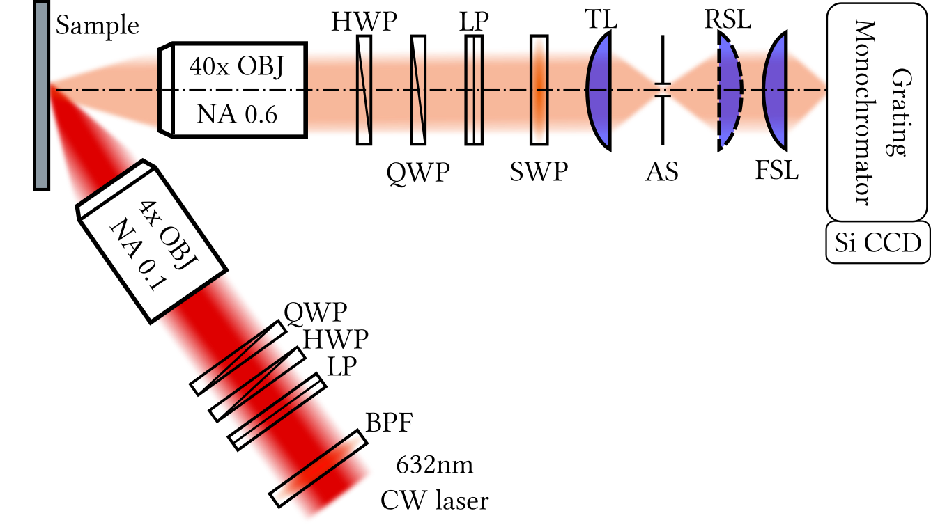
Figure 9: Optical setup used for the angle-resolved polarimetric measurements. See the corresponding paragraph for details.

VIII G: Valley contrast measurements on a bare WS₂ monolayer

The valley contrast $\rho^{\pm}$ of a bare WS₂ monolayer exfoliated on a dielectric substrate (polydimethylsiloxane) is computed from the measured room temperature PL spectra obtained for left and right circular excitations, analysed in the circular basis by a combination of a quarter-wave plate and a Wollaston prism:

$$\rho^{\pm}=\frac{I_{\sigma^{\pm}}(\sigma^{+})-I_{\sigma^{\pm}}(\sigma^{-})}{I_{\sigma^{\pm}}(\sigma^{+})+I_{\sigma^{\pm}}(\sigma^{-})},$$ (14)

where $I_{j}(l)$ is the measured PL spectrum for a $j=(\sigma^{+},\sigma^{-})$ polarized excitation and a $l=(\sigma^{+},\sigma^{-})$ polarized analysis. A typical emission spectrum ($I_{\sigma^{-}}(\sigma^{-})$) is shown in Fig. S10(a) and the valley contrasts $\rho^{\pm}$ are displayed in Fig. S10(b). As discussed in the main text, this emission spectrum consists of a phonon-induced up-converted PL Jones et al. (2016). Clearly, there is no difference in the $I_{j}(l)$ spectra, hence no valley polarization at room temperature on the bare WS₂ monolayer. These results are in striking contrast to those reported in the main text for the strongly coupled system, under similar excitation conditions. Note also that the absence of valley contrast on our bare WS₂ monolayer differs from the results of Nayak et al. (2016) reported however on WS₂ grown by chemical vapor deposition.

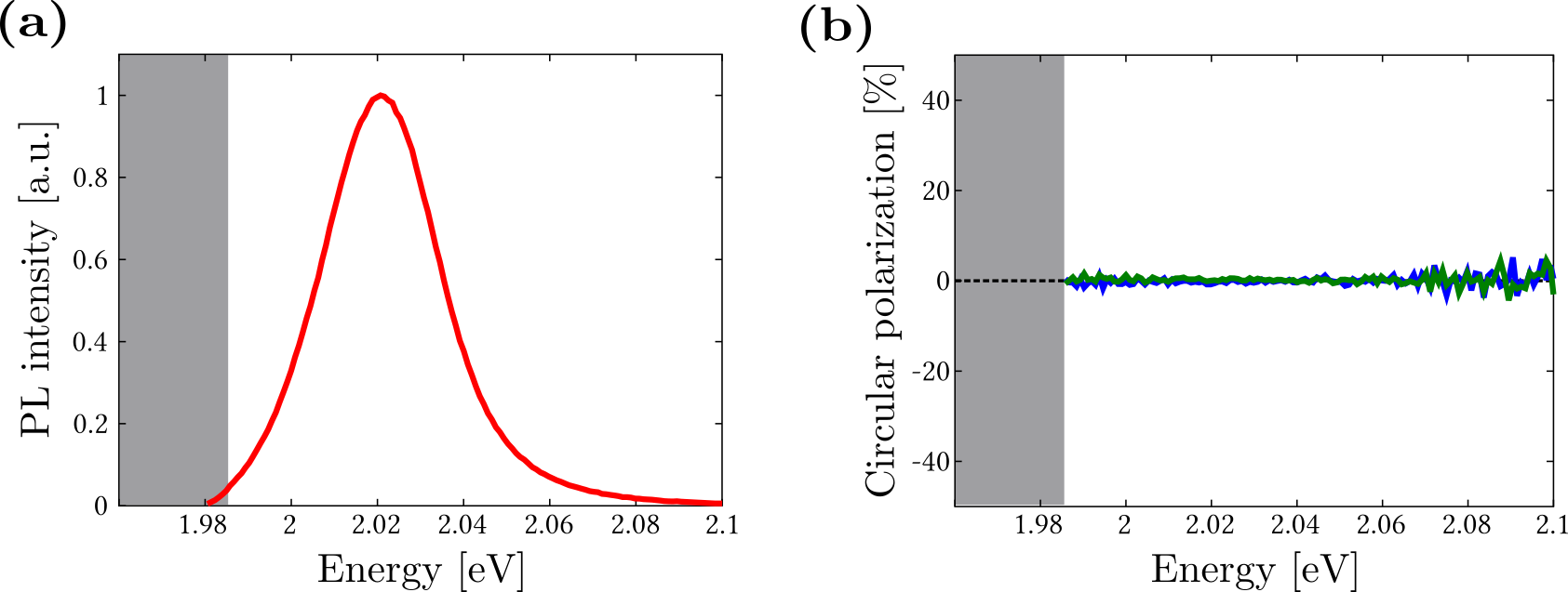
Figure 10: (a) Emission spectrum $I_{\sigma^{-}}(\sigma^{-})$ obtained by exciting the bare WS₂ monolayer at $1.96$ eV with $\sigma^{-}$ polarized light, and analysing the PL in $\sigma^{-}$ polarization. The gray area in (a) and (b) corresponds to the spectral region cut by the PL emission filter. (b) The valley contrast $\rho^{+(-)}$ defined in (14) is displayed in blue (green).

IX H: Angle-resolved Stokes vector polarimetry

The optical setup shown in Fig. S9 is used to measure the angle-resolve PL spectra for different combinations of excitation and detection polarizations. Such measurements allow us to retrieve the coefficients of the Mueller matrix $\mathcal{M}$ of the system, characterizing how the polarization state of the excitation beam affects the polarization state of the chiralitons PL. As discussed in the main text, the spin-momentum locking mechanism of our chiralitonic system relates such PL polarization states to specific chiraliton dynamics. An incident excitation in a given polarization state is defined by a Stokes vector $\bf{S}^{\textrm{\tiny in}}$, on which the matrix $\mathcal{M}$ acts to yield an output PL Stokes vector $\bf{S}^{\textrm{\tiny out}}$:

$$\bf{S}^{\textrm{\tiny out}}=\left(\begin{array}[]{c}I\\ I_{V}-I_{H}\\ I_{45}-I_{-45}\\ I_{\sigma^{+}}-I_{\sigma^{-}}\end{array}\right)_{\textrm{\tiny out}}=\mathcal{M}\left(\begin{array}[]{c}I_{0}\\ I_{V}-I_{H}\\ I_{45}-I_{-45}\\ I_{\sigma^{+}}-I_{\sigma^{-}}\end{array}\right)_{\textrm{\tiny in}},$$ (15)

where $I_{(0)}$ is the emitted (incident) intensity, $I_{V}-I_{H}$ is the relative intensity in vertical and horizontal polarizations, $I_{45}-I_{-45}$ is the relative intensity in $+45^{o}$ and $-45^{o}$ polarizations and $I_{\sigma^{+}}-I_{\sigma^{-}}$ is the relative intensity in $\sigma^{+}$ and $\sigma^{-}$ polarizations. We recall that for our specific alignment of the OSO resonator with respect to the slits of the spectrometer, the angle-resolved PL spectra in $V$ and $H$ polarizations correspond to transverse-magnetic (TM) and transverse-electric (TE) dispersions respectively (see Fig. 2 (b) in the main text). Intervalley chiraliton coherences, revealed by a non-zero degree of linear polarization in the PL upon the same linear excitation, are then measured by the $S_{1}=I_{V}-I_{H}$ coefficient of the PL output Stokes vector. This coefficient is obtained by analysing the PL in the linear basis, giving an angle-resolved PL intensity $\left(S_{0}^{\textrm{\tiny out}}+(-)S_{1}^{\textrm{\tiny out}}\right)/2$, for TM (TE) analysis. In order to obtain the polarization characteristics of the chiralitons, we measure the four possible combinations of excitation and detection polarization in the linear basis:

$$I_{\textrm{\tiny TM/TM}} = \left(m_{00}+m_{01}+m_{10}+m_{11}\right)/2$$ (16)

$$I_{\textrm{\tiny TM/TE}} = \left(m_{00}+m_{01}-m_{10}-m_{11}\right)/2$$ (17)

$$I_{\textrm{\tiny TE/TM}} = \left(m_{00}-m_{01}+m_{10}-m_{11}\right)/2$$ (18)

$$I_{\textrm{\tiny TE/TE}} = \left(m_{00}-m_{01}-m_{10}+m_{11}\right)/2,$$ (19)

where $I_{p/a}$ is the angle-frequency resolved intensity measured for a pump polarization $p=(\textrm{TE,TM})$ and analysed in $a=(\textrm{TE,TM})$ polarization, and $m_{i,j}$ are the coefficients of the 4x4 matrix $\mathcal{M}$. By solving this linear system of equations, we obtain the first quadrant of the Mueller matrix: $m_{00},m_{01},m_{10}$ and $m_{11}$. The $S_{1}^{\textrm{\tiny out}}|_{\textrm{\tiny TM}}$ coefficient of the output Stokes vector for a TM excitation is then directly given by $m_{10}+m_{11}$ as can be seen from (15) by setting $I_{V}=1,I_{H}=0$ and all the other input Stokes coefficients to zeros. This quantity, normalized to $S_{0}^{\textrm{\tiny out}}$, is displayed in the $k_{x}-$energy plane in Fig. 4 (c) in the main text. Similarly, the $S_{1}^{\textrm{\tiny out}}|_{\textrm{\tiny TE}}$ coefficient is given by $m_{10}-m_{11}$, which is the quantity displayed in Fig. 4 (d) in the main text.

As the dispersion of the OSO resonator is different for TE and TM polarizations, the pixel-to-pixel operations performed to obtain $S_{1}^{\textrm{\tiny out}}$ do not directly yield the chiraliton inter-valley contrast. In particular, the observation of negative value regions in $S_{1}^{\textrm{\tiny out}}|_{\textrm{\tiny TM}}$ only reveals that the part of the chiraliton population that lost inter-valley coherence is dominating the total PL in the region of the dispersion where the TE mode dominates over the TM mode (compare Fig. 4(c) and (e)). It does not correspond to genuine anti-correlation of the chiraliton PL polarization with respect to the pump polarization. To correct for such dispersive effects and obtain the degree of chiraliton intervalley coherence, the appropriate quantity is $(S_{1}^{\textrm{\tiny out}}|_{\textrm{\tiny TM}}-S_{1}^{\textrm{\tiny out}}|_{\textrm{\tiny TE}})/(2S_{0}^{\textrm{\tiny out}})=m_{11}$, resolved in the $k_{x}-$energy plane in Fig. 4 (f) in the main text. This quantity can also be refered to as a chiraliton linear depolarization factor. For these polarimetry measurements, the base-line noise was determined by measuring the Mueller matrix associated with an empty setup which are expected to be proportional to the identity matrix. With polarizer extinction coefficients smaller than $0.1\%$, white light (small) intensity fluctuations, and positioning errors of the polarization optics, we reach standard deviations from the identity matrix of the order of $0.4\%$. This corresponds to a base-line noise valid for all the polarimetry measurements presented in the main text. The noise level seen in Fig. 4 in the main text is thus mostly due to fluctuations in the WS₂ PL intensity.

References

- Bliokh et al. (2015) K. Y. Bliokh, F. Rodríguez-Fortuño, F. Nori, and A. V. Zayats, Nat. Photon. 9, 796 (2015).
- Bomzon et al. (2002) Z. Bomzon, G. Biener, V. Kleiner, and E. Hasman, Opt. Lett. 27, 1141 (2002).
- Le Feber et al. (2015) B. Le Feber, N. Rotenberg, and L. Kuipers, Nat. Comm. 6, 6695 (2015).
- Petersen et al. (2014) J. Petersen, J. Volz, and A. Rauschenbeutel, Science 346, 67 (2014).
- Rafayelyan et al. (2016) M. Rafayelyan, G. Tkachenko, and E. Brasselet, Phys. Rev. Lett. 116, 253902 (2016).
- Bliokh et al. (2008a) K. Y. Bliokh, Y. Gorodetski, V. Kleiner, and E. Hasman, Phys. Rev. Lett. 101, 030404 (2008a).
- Gorodetski et al. (2013) Y. Gorodetski, A. Drezet, C. Genet, and T. W. Ebbesen, Phys. Rev. Lett. 110, 203906 (2013).
- Lin et al. (2013) J. Lin, J. B. Mueller, Q. Wang, G. Yuan, N. Antoniou, X.-C. Yuan, and F. Capasso, Science 340, 331 (2013).
- Rodríguez-Fortuño et al. (2013) F. J. Rodríguez-Fortuño, G. Marino, P. Ginzburg, D. O’Connor, A. Martínez, G. A. Wurtz, and A. V. Zayats, Science 340, 328 (2013).
- Spektor et al. (2015) G. Spektor, A. David, B. Gjonaj, G. Bartal, and M. Orenstein, Nano Lett. 15, 5739 (2015).
- Jiang et al. (2016) Q. Jiang, A. Pham, M. Berthel, S. Huant, J. Bellessa, C. Genet, and A. Drezet, ACS Photon. 3, 1116 (2016).
- O’Connor et al. (2014) D. O’Connor, P. Ginzburg, F. J. Rodríguez-Fortuño, G. A. Wurtz, and A. V. Zayats, Nat. Comm. 5, 5327 (2014).
- Mitsch et al. (2014) R. Mitsch, C. Sayrin, B. Albrecht, P. Schneeweiss, and A. Rauschenbeutel, Nat. Comm. 5, 5713 (2014).
- Junge et al. (2013) C. Junge, D. O’Shea, J. Volz, and A. Rauschenbeutel, Phys. Rev. Lett. 110, 213604 (2013).
- Söllner et al. (2015) I. Söllner, S. Mahmoodian, S. L. Hansen, L. Midolo, A. Javadi, G. Kiršanskė, T. Pregnolato, H. El-Ella, E. H. Lee, J. D. Song, S. Stobbe, and P. Lodahl, Nat. Nano. 10, 775 (2015).
- Gonzalez-Ballestro et al. (2015) C. Gonzalez-Ballestro, A. Gonzalez-Tudela, F. J. Garcia-Vidal, and E. Moreno, Phys. Rev. B 92, 155304 (2015).
- Sayrin et al. (2015) C. Sayrin, C. Junge, R. Mitsch, B. Albrecht, D. O’Shea, P. Schneeweiss, J. Volz, and A. Rauschenbeutel, Phys. Rev. X 5, 041036 (2015).
- Young et al. (2015) A. B. Young, A. C. T. Thijssen, D. M. Beggs, P. Androvitsaneas, L. Kuipers, J. G. Rarity, S. Hughes, and R. Oulton, Phys. Rev. Lett. 115, 153901 (2015).
- Gonzalez-Ballestro et al. (2016) C. Gonzalez-Ballestro, E. Moreno, F. J. Garcia-Vidal, and A. Gonzalez-Tudela, Phys. Rev. A 94, 063817 (2016).
- Coles et al. (2016) R. J. Coles, D. M. Price, J. E. Dixon, B. Royall, E. Clarke, P. Kok, M. S. Skolnick, A. M. Fox, and M. N. Makhonin, Nat. Comm. 7, 11183 (2016).
- Lodahl et al. (2017) P. Lodahl, S. Mahmoodian, S. Stobbe, P. Schneeweiss, J. Volz, A. Rauschenbeutel, H. Pichler, and P. Zoller, Nature 541, 473 (2017).
- Jones et al. (2013) A. M. Jones, H. Yu, N. J. Ghimire, S. Wu, G. Aivazian, J. S. Ross, B. Zhao, J. Yan, D. G. Mandrus, D. Xiao, W. Yao, and X. Xu, Nat. Nano. 8, 634 (2013).
- Moody et al. (2016) G. Moody, J. Schaibley, and X. Xu, J. Opt. Soc. Am. B 33, C39 (2016).
- Hao et al. (2016) K. Hao, G. Moody, F. Wu, C. K. Dass, L. Xu, C.-H. Chen, L. Sun, M.-Y. Li, L.-J. Li, A. H. MacDonald, and X. Li, Nat. Phys. Advance Online Publication (2016), 10.1038/nphys3674.
- Dufferwiel et al. (2017) S. Dufferwiel, T. P. Lyons, D. D. Solnyshkov, A. A. P. Trichet, F. Withers, S. Schwarz, G. Malpuech, J. M. Smith, K. S. Novoselov, M. S. Skolnick, D. N. Krizhanovskii, and A. I. Tartakovskii, Nat. Photon. 11, 497 (2017).
- Chen et al. (2017) Y.-J. Chen, J. D. Cain, T. K. Stanev, V. P. Dravid, and N. P. Stern, Nat. Photon. 11, 431 (2017).
- Kleemann et al. (2017) M.-E. Kleemann, R. Chikkaraddy, E. M. Alexeev, D. Kos, C. Carnegie, W. Deacon, A. de Casalis de Pury, C. Grosse, B. de Nijs, J. Mertens, A. I. Tartakovskii, and J. J. Baumberg, https://arxiv.org/abs/1704.02756 (2017), arXiv:1704.02756 [physics.optics.
- Liu et al. (2015) X. Liu, T. Galfsky, Z. Sun, F. Xia, E.-C. Lin, Y.-H. Lee, S. Kéna-Cohen, and V. M. Menon, Nat. Photon. 9, 30 (2015).
- Dufferwiel et al. (2015) S. Dufferwiel, S. Schwarz, F. Withers, A. A. P. Trichet, F. Li, M. Sich, O. Del Pozo-Zamudio, C. Clark, A. Nalitov, D. D. Solnyshkov, G. Malpuech, K. S. Novoselov, J. M. Smith, M. S. Skolnick, D. N. Krizhanovskii, and A. I. Tartakovskii, Nat. Comm. 6, 8579 (2015).
- Sidler et al. (2017) M. Sidler, P. Back, O. Cotlet, A. Srivastava, T. Fink, M. Kroner, E. Demler, and A. Imamoǧlu, Nat. Phys. 13, 255 (2017).
- Liu et al. (2016) W. Liu, B. Lee, C. H. Naylor, H.-S. Ee, J. Park, A. T. C. Johnson, and R. Agarwal, Nano Lett. 16, 1262 (2016).
- Wang et al. (2016a) S. Wang, S. Li, T. Chervy, A. Shalabney, S. Azzini, E. Orgiu, J. A. Hutchison, C. Genet, P. Samorì, and T. W. Ebbesen, Nano Lett. 16, 4368 (2016a).
- Li et al. (2014) Y. Li, A. Chernikov, X. Zhang, A. Rigosi, H. M. Hill, A. M. van der Zande, D. A. Chenet, E.-M. Shih, J. Hone, and T. F. Heinz, Phys. Rev. B 90, 205422 (2014).
- Mak and Shan (2016) K. F. Mak and J. Shan, Nat. Photon. 10, 216 (2016).
- Li et al. (2017) Z. Li, Y. Li, T. Han, X. Wang, Y. Yu, B. Tay, Z. Liu, and Z. Fang, ACS Nano 11, 1165 (2017).
- Gong et al. (2017) S.-H. Gong, F. Alpeggiani, B. Sciacca, E. C. Garnett, and L. Kuipers, https://arxiv.org/abs/1709.00762 (2017), arXiv:1704.02756 [physics.optics].
- Bliokh et al. (2008b) K. Y. Bliokh, Y. Gorodetski, V. Kleiner, and E. Hasman, Phys. Rev. Lett. 101, 030404 (2008b).
- Shitrit et al. (2011) N. Shitrit, I. Bretner, Y. Gorodetski, V. Kleiner, and E. Hasman, Nano Lett. 11, 2038 (2011).
- Huang et al. (2013) L. Huang, X. Chen, B. Bai, Q. Tan, G. Jin, T. Zentgraf, and S. Zhang, Light Sci. Appl. 2 (2013), 10.1038/lsa.2013.26.
- Houdré (2005) R. Houdré, Physica Status Solidi (b) 242, 2167 (2005).
- Törmä and Barnes (2015) P. Törmä and W. L. Barnes, Reports on Progress in Physics 78, 013901 (2015).
- Seyler et al. (2015) K. L. Seyler, J. R. Schaibley, P. Gong, P. Rivera, A. M. Jones, S. Wu, J. Yan, D. G. Mandrus, W. Yao, and X. Xu, Nat. Nano. 10, 407 (2015).
- Hanbicki et al. (2016) A. T. Hanbicki, K. M. McCreary, G. Kioseoglou, M. Currie, C. S. Hellberg, A. L. Friedman, and B. T. Jonker, AIP Advances 6, 055804 (2016), http://dx.doi.org/10.1063/1.4942797 .
- Jones et al. (2016) A. M. Jones, H. Yu, J. R. Schaibley, J. Yan, D. G. Mandrus, T. Taniguchi, K. Watanabe, H. Dery, W. Yao, and X. Xu, Nat. Phys. 12, 323 (2016).
- Whittaker et al. (1996) D. M. Whittaker, P. Kinsler, T. A. Fisher, M. S. Skolnick, A. Armitage, A. M. Afshar, M. D. Sturge, and J. S. Roberts, Phys. Rev. Lett. 77, 4792 (1996).
- Wang et al. (2016b) G. Wang, X. Marie, B. L. Liu, T. Amand, C. Robert, F. Cadiz, P. Renucci, and B. Urbaszek, Phys. Rev. Lett. 117, 187401 (2016b).
- Schmidt et al. (2016) R. Schmidt, A. Arora, G. Plechinger, P. Nagler, A. Granados del Aguila, M. V. Ballottin, P. C. M. Christianen, S. Michaelis de Vasconcellos, C. Schuller, T. Korn, and R. Bratschitsch, Phys. Rev. Lett. 117, 077402 (2016).
- Ye et al. (2017) Z. Ye, D. Sun, and T. F. Heinz, Nat. Phys. 13, 26 (2017).
- Zhu et al. (2014) B. Zhu, H. Zeng, J. Dai, Z. Gong, and X. Cui, PNAS 111, 11606 (2014).
- Low et al. (2017) T. Low, A. Chaves, J. D. Caldwell, A. Kumar, N. X. Fang, P. Avouris, T. F. Heinz, F. Guinea, L. Martin-Moreno, and F. Koppens, Nat. Mater. 16, 182 (2017).
- Ciuti et al. (2005) C. Ciuti, G. Bastard, and I. Carusotto, Phys. Rev. B 72, 115303 (2005).
- Holmes and Forrest (2004) R. J. Holmes and S. R. Forrest, Phys. Rev. Lett. 93, 186404 (2004).
- Federspiel et al. (2015) F. Federspiel, G. Froehlicher, M. Nasilowski, S. Pedetti, A. Mahmood, B. Doudin, S. Park, J.-O. Lee, D. Halley, B. Dubertret, P. Gilliot, and S. Berciaud, Nano Lett. 15, 1252 (2015).
- Pöllmann et al. (2015) C. Pöllmann, P. Steinleitner, U. Leierseder, P. Nagler, G. Plechinger, M. Porer, R. Bratschitsch, C. Schüller, T. Korn, and R. Huber, Nat. Mater. 14, 889 (2015).
- Robert et al. (2016) C. Robert, D. Lagarde, F. Cadiz, G. Wang, B. Lassagne, T. Amand, A. Balocchi, P. Renucci, S. Tongay, B. Urbaszek, and X. Marie, Phys. Rev. B 93, 205423 (2016).
- Heinz et al. (1982) T. F. Heinz, C. K. Chen, D. Ricard, and Y. R. Shen, Phys. Rev. Lett. 48, 478 (1982).
- Chervy et al. (2016) T. Chervy, J. Xu, Y. Duan, C. Wang, L. Mager, M. Frerejean, J. A. Munninghoff, P. Tinnemans, J. A. Hutchison, C. Genet, A. Rowan, T. Rasing, and T. W. Ebbesen, Nano Lett. 16, 7352 (2016).
- Lin et al. (1993) S. H. Lin, R. G. Alden, A. A. Villaeys, and V. Pflumio, Phys. Rev. A 48, 3137 (1993).
- Nayak et al. (2016) P. K. Nayak, F.-C. Lin, C.-H. Yeh, J.-S. Huang, and P.-W. Chiu, Nanoscale 8, 6035 (2016).