Isotope effect on filament dynamics in fusion edge plasmas

Abstract

The influence of the ion mass on filament propagation in the scrape-off layer of toroidal magnetised plasmas is analysed for various fusion relevant majority species, like hydrogen isotopes and helium, on the basis of a computational isothermal gyrofluid model for the plasma edge. Heavy hydrogen isotope plasmas show slower outward filament propagation and thus improved confinement properties compared to light isotope plasmas, regardless of collisionality regimes. Similarly, filaments in fully ionised helium move more slowly than in deutrium. Different mass effects on the filament inertia through polarisation, finite Larmor radius, and parallel dynamics are identified.

Keywords: isotope effect, plasma filament, blob, particle transport

1 Introduction

In various tokamak experiments the confinement properties have been shown to scale favourably with increasing mass of the main (fusion relevant) ion plasma species, specifically hydrogen isotopes and helium [1, 2, 3, 4]. The radial cross-field transport of coherent filamentary structures (commonly denoted “blobs”) in the scrape-off layer (SOL) of tokamaks accounts for a significant part of particle and heat losses [5, 6] to the plasma facing components. Experimentally the ion mass effect on SOL filament dynamics has been studied in a simple magnetised torus [7]. Filamentary transport in tokamaks in general is an active subject of studies in experiments, analytical theory, and by computations in two and three dimensions.

The basic properties of filamentary transport are reviewed in [8]. Blob propagation results from magnetic drifts that polarise density perturbations, thus yielding a dipolar electric potential $\phi$ whose resulting ${\bf B}\times\nabla\phi$ drift in the magnetic field ${\bf B}$ drives the filaments down the magnetic field gradient and towards the wall. The basic physics is illustrated by accounting for the current paths involved upon charging of the blob by the diamagnetic current: the closure is via perpendicular polarisation currents in the drift plane and through parallel divergence of the parallel current [9].

Two-dimensional (2-d) closure schemes are discussed in Ref. [10]. Depending on parallel resistivity, the dominant closure path features distinct dynamics: if closure is mainly through the polarisation current, the 2-d cross-field properties are dominant, leading to a mushroom-cape shaped radial propagation. For reduced resistivity the closure parallel to the magnetic field direction in 3-d is dominant, and Boltzmann spinning leads to a more coherently propagating structure at significantly reduced radial velocity.

The isotope mass may have influence on the ${\bf E}\times{\bf B}$ shearing rate in the edge region [11], and flow shear in the edge region has been suggested to be a main agent which controls blob formation [12]. In addition, a finite ion temperature introduces poloidally asymmetric propagation of blobs [13, 14]. The underlying finite Larmor radius (FLR) effects have been found to contribute to favourable isotopic transport scaling of tokamak edge turbulence [15].

In this work we study the isotopic mass effect on blob filament propagation by employing an isothermal gyrofluid model so that relevant FLR contributions to the blob evolution are effectively included, in addition to the mass dependencies in polarisation and in parallel ion velocities.

2 Gyrofluid model and computation

The present simulations on the isotopic dependence of 3-d filament and 2-d blob propagation in the edge and SOL of tokamaks are based on the gyrofluid electromagnetic model introduced by Scott [16]. In the local delta-$f$ isothermal limit the model consists of evolution equations for the gyrocenter densities $n_{s}$ and parallel velocities $u_{s\shortparallel}$ of electrons and ions, where the index $s$ denotes the species with $s\in(\mathrm{e},i)$:

$$\frac{\rmd_{s}n_{s}}{\rmd t}= -\nabla_{\shortparallel}u_{s\shortparallel}+\mathcal{K}\left(\phi_{s}+\tau_{s}n_{s}\right),$$ (1)

$$\widehat{\beta}\;\frac{\partial A_{\shortparallel}}{\partial t}+\epsilon_{s} \frac{\rmd_{s}u_{s\shortparallel}}{\rmd t}= -\nabla_{\shortparallel}\left(\phi_{s}+\tau_{s}n_{s}\right)+2\epsilon_{s}\tau_{s}\mathcal{K}\left(u_{s\shortparallel}\right)-CJ_{\shortparallel},$$ (2)

The gyrofluid moments are coupled by the polarisation equation

$$\sum_{s}a_{s}\left[\Gamma_{1}n_{s}+\frac{\Gamma_{0}-1}{\tau_{s}}\phi\right]=0,$$ (3)

and Ampere’s law

$$-\nabla_{\perp}^{2}A_{\shortparallel}=J_{\shortparallel}=\sum_{s}a_{s}u_{s\shortparallel}.$$ (4)

The gyroscreened electrostatic potential acting on the ions is given by

$$\phi_{s}=\Gamma_{1}\left(\rho_{s}^{2}k_{\perp}^{2}\right)\widehat{\phi}_{\mathbf{k}},$$

where $\widehat{\phi}_{\mathbf{k}}$ are the Fourier coefficients of the electrostatic potential. The gyroaverage operators $\Gamma_{0}(b)$ and $\Gamma_{1}(b)=\Gamma_{0}^{1/2}(b)$ correspond to multiplication of Fourier coefficients by $I_{0}(b)e^{-b}$ and $I_{0}(b/2)e^{-b/2}$, respectively, where $I_{0}$ is the modified Bessel function of zero’th order and $b=\rho_{s}^{2}k_{\perp}^{2}$. We here use approximate Padé forms with $\Gamma_{0}(b)\approx(1+b)^{-1}$ and $\Gamma_{1}(b)\approx(1+b/2)^{-1}$ [17].

The perpendicular $\mathbf{E}\times\mathbf{B}$ advective and the parallel derivative operators for species $s$ are given by

$$\frac{\rmd_{s}}{\rmd t}=\frac{\partial}{\partial t}+\delta^{-1}\left\{\phi_{s},~{}\right\},$$

$$\nabla_{\shortparallel}=\frac{\partial}{\partial z}-\delta^{-1}\widehat{\beta}\left\{A_{\shortparallel},~{}\right\},$$

where we have introduced the Poisson bracket as

$$\left\{f,g\right\}=\left(\frac{\partial f}{\partial x}\frac{\partial g}{\partial y}-\frac{\partial f}{\partial y}\frac{\partial g}{\partial x}\right).$$

In local three-dimensional flux tube co-ordinates $\{x,y,z\}$, $x$ is a (radial) flux-surface label, $y$ is a (perpendicular) field line label and $z$ is the position along the magnetic field line. In circular toroidal geometry with major radius $R$, the curvature operator is given by

$$\mathcal{K}=\omega_{B}\left(\sin z\;\frac{\partial}{\partial x}+\cos z\;\frac{\partial}{\partial y}\right),$$

where $\omega_{B}=2L_{\perp}/R$, and the perpendicular Laplacian is given by

$$\nabla_{\perp}^{2}=\left(\frac{\partial^{2}}{\partial x^{2}}+\frac{\partial^{2}}{\partial y^{2}}\right).$$

Flux surface shaping effects [18, 19] in more general tokamak or stellarator geometry on SOL filaments [20] are here neglected for simplicity.

Spatial scales are normalised by the drift scale $\rho_{0}=\sqrt{T_{\rme}m_{i0}}/\rme B$, where $T_{\rme}$ is a reference electron temperature, $B$ is the reference magnetic field strength and $m_{i0}$ is a reference ion mass, for which we use the mass of deuterium $m_{i0}=m_{\mathrm{D}}$. The temporal scale is set to by $c_{0}/L_{\perp}$, where $c_{0}=\sqrt{T_{\rme}/m_{i0}}$, and $L_{\perp}$ is a perpendicular normalisation length (e.g. a generalized profile gradient scale length), so that $\delta=\rho_{0}/L_{\perp}$ is the drift scale. The temporal scale may be expressed alternatively $L_{\perp}/c_{0}=L_{\perp}/(\rho_{0}\Omega_{0})=(\delta\Omega_{0})^{-1}$, with the ion-cyclotron frequency $\Omega_{0}=\rho_{0}/c_{0}$. In the following we employ $\delta=0.01$.

The main species dependent parameters are

$$a_{s}=\frac{Z_{s}n_{s0}}{n_{\rme 0}},\quad\tau_{s}=\frac{T_{s}}{Z_{s}T_{\rme}},\quad\mu_{s}=\frac{m_{s}}{Z_{s}m_{i0}},$$

$$\rho_{s}^{2}=\mu_{s}\tau_{s}\rho_{0}^{2},\quad\epsilon_{s}=\mu_{s}\left(\frac{qR}{L_{\perp}}\right)^{2},$$

setting the relative concentrations, temperatures, mass ratios and FLR scales of the respective species. $Z_{s}$ is the charge state of the species $s$ with mass $m_{s}$ and temperature $T_{s}$.

The plasma beta parameter

$$\widehat{\beta}=\frac{4\pi p_{\rme}}{B^{2}}\left(\frac{qR}{L_{\perp}}\right)^{2},$$

controls the shear-Alfvén activity, and

$$C=0.51\frac{\nu_{\rme}L_{\perp}}{c_{0}}\frac{m_{\rme}}{m_{i0}}\left(\frac{qR}{L_{\perp}}\right)^{2},$$

mediates the collisional parallel electron response for $Z=1$ charged hydrogen isotopes. The collisional response for other isotopes or ion species is discussed further below.

Parallel boundary conditions

We distinguish between two settings for parallel boundary conditions in 3-d simulations. In the case of edge simulations a toroidal closed-flux-surface (CFS) geometry is considered, and quasi-periodic globally consistent flux-tube boundary conditions in the parallel direction [21] are applied on both state-variables $n_{\rme},\phi$ and flux variables $v_{\rme\shortparallel},u_{s\shortparallel}$.

For SOL simulations, the state variables assume zero-gradient Neumann (sheath) boundary conditions at the limiter location, and the flux variables are given as

$$u_{s\shortparallel}|_{\pm\pi} =p_{\rme}|_{\pm\pi}=\pm\Gamma_{d}n_{\rme}|_{\pm\pi},$$ (5)

$$v_{\rme\shortparallel} =u_{s\shortparallel}|_{\pm\pi}-J_{\shortparallel}|_{\pm\pi}=\pm\Gamma_{d}[(\Lambda+1)n_{\rme}|_{\pm\pi}-\phi|_{\pm\pi}],$$ (6)

at the parallel boundaries $z=\pm\pi$ respectively [22]. Note that in order to retain the Debye sheath mode in this isothermal model, the Debye current $J_{\shortparallel}|_{\pm\pi}=\pm\Gamma_{d}(\phi-\Lambda T_{\rme})$ is expressed as $J_{\shortparallel}|_{\pm\pi}=\pm\Gamma_{d}(\phi-\Lambda n_{\rme})$ and the electron pressure $p_{\rme}=n_{\rme}T_{\rme}$ is replaced by $p_{\rme}=n_{\rme}$ [22]. This edge/SOL set-up and its effects on drift wave turbulence has been presented in detail by Ribeiro et alin Refs. [22, 23].

The sheath coupling constant is $\Gamma_{d}=\sqrt{(1+\tau_{i})/(\mu_{i}\widehat{\epsilon})}$. The floating potential is given by $\Lambda=\Lambda_{0}+\Lambda_{i}$, where $\Lambda_{0}=\log\sqrt{m_{i0}/(2\pi m_{\rme})}$ and $\Lambda_{i}=\log\sqrt{\mu_{i}/(1+\tau_{i})}$. Here terms with the index $i$ apply only to the ion species. The expressions presented here are obtained by considering the finite ion temperature acoustic sound speed, $c_{i}=\sqrt{(Z_{i}T_{i}+T_{\rme})/m_{i}}$, instead of $c_{0}$ in Ref. [22]. This results in the additional $\Lambda_{i}$, and the normalisation scheme yields the extra $\sqrt{(1+\tau_{i})/\mu_{i}}$ in $\Gamma_{d}$.

Numerical implementation

Our code TOEFL [24] is based on the delta-$f$ isothermal electromagnetic gyrofluid model [16] and uses globally consistent flux-tube geometry [21] with a shifted metric treatment of the coordinates [25] to avoid artefacts by grid deformation. In the SOL region a sheath boundary condition model is applied [22, 23]. The electrostatic potential is obtained from the polarisation equation by an FFT Poisson solver with zero-Dirichlet boundary conditions in the (radial) $x$-direction. Gyrofluid densities are adapted at the $x$-boundaries to ensure zero vorticity radial boundary conditions for finite ion temperature. An Arakawa-Karniadakis scheme is employed for advancing the moment equations [26, 27, 28].

3 Scaling laws from dimensional analysis

Blob velocity scalings are commonly deduced from the fluid vorticity equation. We follow this approach and construct the gyrofluid vorticity equation to deduce velocity scaling laws. The vorticity equation can be obtained upon expressing the gyrocenter ion density in terms of the electron density and polarisation contribution, inserting in the ion gyrocenter density evolution equation and subtracting the electron density evolution equation [14, 29]. Up to $\mathcal{O}(b)$ the ion gyrocenter density is

$$n_{i}=n_{\rme}-\frac{1}{2}\mu_{i}\nabla_{\perp}^{2}p_{i}-\mu_{i}\nabla_{\perp}^{2}\phi,$$ (7)

where the ion pressure is given in terms of the electron particle density $p_{i}=\tau_{i}n_{\rme}$. The gyroaveraged potential for species $s$ up to $\mathcal{O}(b)$ is

$$\phi_{s}=\phi+\frac{1}{2}\mu_{i}\tau_{i}\nabla_{\perp}^{2}\phi.$$ (8)

Following Ref. [29] we obtain

$$\mu_{i}\nabla\cdot\frac{\rmd}{\rmd t}\nabla_{\perp}\phi^{*}=\nabla_{\shortparallel}J_{\shortparallel}-(1+\tau_{i})\mathcal{K}(n_{\rme}).$$ (9)

Here we have introduced the modified potential $\phi^{*}=\phi+p_{i}$. The vorticity equation is equivalent to the quasi-neutrality statement of current continuity, $\nabla\cdot\mathbf{J}=0$. We identify the divergence of the polarisation current,

$$\nabla\cdot\mathbf{J}_{\mathrm{pol}}=-\mu_{i}\nabla\cdot\frac{\rmd}{\rmd t}\nabla_{\perp}\phi^{*},$$ (10)

and the divergence of the diamagnetic current,

$$\nabla\cdot\mathbf{J}_{\mathrm{dia}}=-(1+\tau_{i})\mathcal{K}(n_{\rme}).$$ (11)

Blob propagation has in a linearisation of the present gyrofluid model been analytically analysed by Manz et alin Ref. [30]. Therein the dependence of blob velocity on the ion isotope mass is in principle present but not explicitly apparent. To clarify, we here restate the calculations of Ref. [30], but use the vorticity eq. (9) with the explicit occurence of $\mu_{i}$. Neglecting parallel currents, employing the blob correspondence $\partial_{x},\partial_{y}\rightarrow 1/\sigma$ and $\rmd/\rmd t\rightarrow i\gamma=iv_{b}/\sigma$ [31], in terms of the blob width $\sigma$, blob velocity $v_{b}$ and linear growth rate of the instability $\gamma$ and furthermore identifying $\phi=iv_{b}\sigma$ (the radial component of the electric drift), we get (in normalised units):

$$v_{b}=\frac{1}{\sqrt{2}}\sqrt{\sqrt{f^{2}+g^{2}}-f},~{}\mathrm{where}~{}f=\left(\frac{\tau_{i}A}{2\sigma}\right)^{2},~{}g=\frac{1+\tau_{i}}{\mu_{i}}\omega_{B}\sigma A.$$ (12)

$A$ is the initial blob amplitude. In the limit of large blobs, $g\gg f$, so that

$$v_{b}\approx\frac{1}{\sqrt{2}}\sqrt{\frac{1+\tau_{i}}{\mu_{i}}\omega_{B}\sigma A},$$ (13)

and for smaller blobs satisfying $g\ll f$ we get

$$v_{b}\approx\frac{1+\tau_{i}}{\tau_{i}}\frac{\omega_{B}\sigma^{2}}{\mu_{i}}.$$ (14)

The correspondence with the result of Ref. [30] is made explicit upon renormalising, i.e. letting $v_{b}\rightarrow v_{b}/\delta c_{0},A\rightarrow A/\delta,\sigma\rightarrow\sigma/\rho_{0},\omega_{B}\rightarrow 2L_{\perp}/R$. The limits then are

$$v_{b}\approx\sqrt{\frac{1+\tau_{i}}{\mu_{i}}}c_{0}\sqrt{\frac{2\sigma}{R}A},~{}\mathrm{for}~{}\sigma^{3}\gg\frac{\mu_{i}\tau_{i}^{2}A}{4(1+\tau_{i})\omega_{B}},$$ (15)

and

$$v_{b}\approx 2\frac{c_{0}}{\mu_{i}}\frac{1+\tau_{i}}{\tau_{i}}\left(\frac{\sigma}{\rho_{0}}\right)^{2},~{}\mathrm{for}~{}\sigma^{3}\ll\frac{\mu_{i}\tau_{i}^{2}A}{4(1+\tau_{i})\omega_{B}}.$$ (16)

For 2-d computations of sufficiently large blobs we consequently expect $v_{b}\sim 1/\sqrt{\mu_{i}}$, whereas for the 3-d model the expected scaling is not a priori that clear. In Ref. [30] 3-d (linear) scaling laws were presented, where the parallel dynamics was approximated by the Hasegawa-Wakatani closure, $\nabla_{\shortparallel}J_{\shortparallel}=\frac{1}{C}\nabla_{\shortparallel}^{2}(n_{\rme}-\phi)$.

In the following we are going to compare reduced 2-d and full 3-d dynamical blob simulations for various isotope species with the analytical $1/\sqrt{\mu_{i}}$-scaling.

4 Two-dimensional blob computations

In this section we numerically analyse the dependence ob filament dynamics on the normalised ion mass $\mu_{i}$ by reduced 2-d blob simulations of the isothermal gyrofluid eqs. (1,2). For the computations in this section we us as parameters: curvature $\omega_{B}=0.05$, drift scale $\delta=0.01$, grid size $L_{y}=128\rho_{s}$, grid points $N_{x}=N_{y}=256$, initial blob amplitude $A=1$ and Gaussian blob width $\sigma=10\rho_{s}$.

Fig. 1 shows contours plots of the electron particle density at different times of evolution of a seeded blob for several species of cold ions ($\tau_{i}=0$). The initial Gaussian density perturbation $n_{e}(x,y,t=0)=A\exp\left[-(x^{2}+y^{2})/\sigma^{2}\right]$ undergoes the familiar transition towards a mushroom-shaped structure before the blob eventually breaks up due to secondary instabilities. This figure illustrates the main point for the following discussion: lighter isotopes propagate faster than heavier isotopes. In terms of the (normalising) deuterium mass we consider $\mu_{\mathrm{H}}=1/2$, $\mu_{\mathrm{D}}=1$, $\mu_{\mathrm{T}}=3/2$ and $\mu_{\mathrm{He+}}=2$ with $\mu_{i}=m_{i}/(Z_{i}m_{D})$. The species index $\mathrm{He+}$ here denotes singly charged helium-4 with $Z_{He+}\equiv 1$. The case of (fully ionised) doubly charged helium-4 isotopes will be discussed further below in context of 3-d simulations in Sec. 5.0.2. Note that the lighter the ion species are, the further the blob is developed in its radial propagation and evolution at a given snapshot in time.

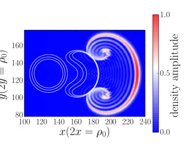
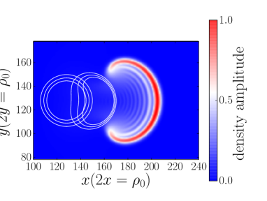
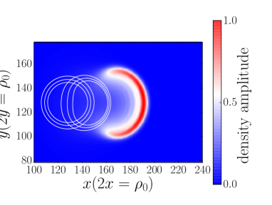
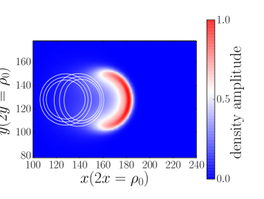
Figure 1: Electron density contour plots of 2-d cold ion ($\tau_{i}=0$) show the different blob propagation for several plasma species. White contour lines are snapshots at $t=0$, and at $t=3$. The colour plot is drawn at $t=6$. Isoptopes: protium (top left), deuterium (top right), tritium (bottom left) and singly charged helium-4 (bottom right).

For warm ions ($\tau_{i}>0$) the blob propagation depends on the relative initialisation of the electron and ion gyrocenter densities. Commonly, a zero ${\bf E}\times{\bf B}$ vorticity blob initialisation is assumed where $n_{i}(x,y,t=0)=\Gamma_{1}^{-1}n_{\rme}(x,y,t=0)$: inserting these into the polarisation eq. (3) results in vorticity $\Omega\equiv\nabla_{\perp}^{2}\phi=0$. This initialisation for most parameters leads to an FLR induced rapid development of a perpendicular propagation component in addition to the radial propagation of the blob, and thus a pronounced up-down asymmetry in $y$ direction. Alternatively, the electron and ion gyrocenter densities can be chosen as equal with $n_{i}(x,y,t=0)=n_{e}(x,y,t=0)$, so that $\phi\sim n_{e}$. In this case the initial vorticity mostly cancels the FLR asymmetry effect, and the blob remains more coherent and steady in its radial propagation [32]. The truth may be somewhere in between: as in the experiment blobs are not “seeded” (in contrast to common simulations), but appear near the separatrix from ${\bf E}\times{\bf B}$ drift wave vortices or are sheared off from poloidal flows, in general some phase-shifted combination of electric potential and density perturbations will appear. For comparison we perform simulations with both of these seeded blob density initialisations.

We note that the $x$ coordinate is effectively pointing radially outwards (in negative magnetic field gradient direction) at a low-field midplane location in a tokamak, and the magnetic field here points into the ($x,y$) plane (${\bf e}_{z}={\bf e}_{y}\times{\bf e}_{x}$), so that the effective electron diamagnetic drift direction of poloidal propagation is in the present plots downwards (in negative $y$ direction).

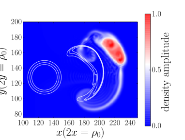
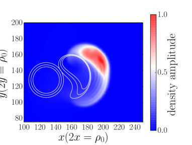
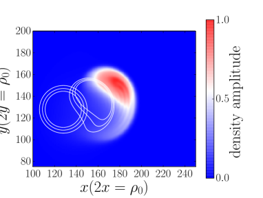
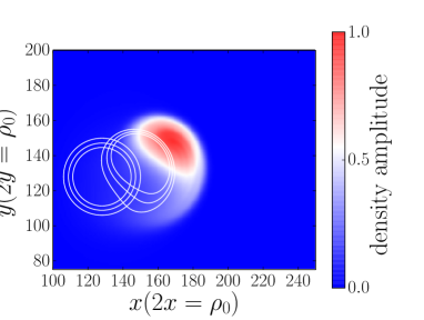
Figure 2: Electron density contour plots of 2-d warm ion ($\tau_{i}=1$) blob propagation for different plasma species, using zero-vorticity initial conditions. White contour lines are snapshots at $t=0$, and at $t=3$; the colour plot is at $t=6$. Protium (top left), deuterium (top right), tritium (bottom left) and singly charged helium-4 (bottom right).

Fig. 2 shows blob propagation for warm ions with $\tau_{i}=1$, initialised with the zero vorticity condition. For comparison, we present in Fig. 3 the propagation for the same parameters but initialised with equal electron and ion gyrocenter densities. Clearly, the latter cases with initial non-zero vorticity $\Omega=\nabla_{\perp}^{2}\phi$ results in faster and more coherent radial propagation, whereas the zero vorticity cases exhibit significant poloidal translation through the FLR induced spin-up. Regardless of initialisation, blobs of light ion species with small $\mu_{i}$ travel faster and are further developed at a given time compared to heavier species.

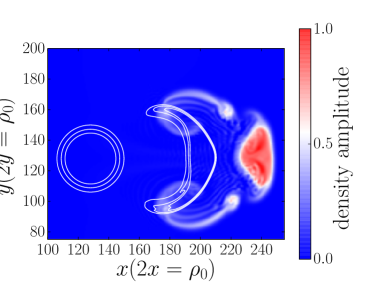
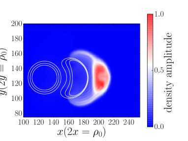
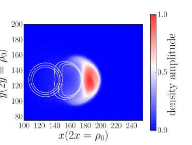
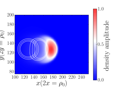
Figure 3: Electron density contour plots of 2-d warm ion ($\tau_{i}=1$) blob propagation for different plasma species, using non-zero vorticity initial conditions. White contour lines are snapshots at $t=0$, and at $t=3$; the colour plot is at $t=6$. Protium (top left), deuterium (top right), tritium (bottom left) and singly charged helium-4 (bottom right).

Relevant quantities which determine the intermittent blob related transport properties of the tokamak SOL are the maximum blob velocity and acceleration. In Fig. 4 we present maximum radial center-of-mass velocities $V_{x,\mathrm{max}}$ and the average radial acceleration $A$ as a function of the the ion mass parameter $\mu_{i}$. The different symbols/colours represent cases with cold ($\tau_{i}=0$, blue lower curves) and warm ($\tau_{i}=1$) ions, with both types of initial conditions used on the latter: the zero vorticity condition is depicted in red (middle curves) and the $n_{e}=n_{i}$ condition in green (upper curves).

It can be seen that the maximum radial blob velocity is slightly larger for $n_{e}=n_{i}$ initialisation due to the mainly radial propagation (left figure), but the average acceleration is for both cases nearly equal (right figure).

The radial center-of-mass position is given by $X_{\mathrm{c}}=[\int\rmd x\rmd y~{}xn_{\rme}]/[\int\rmd x\rmd y~{}n_{\rme}]$. Taking the temporal derivative gives the radial center-of-mass velocity, $V_{x}=\rmd X_{\mathrm{c}}/\rmd t$. The maximum of $V_{x}(t)$, $V_{x,\mathrm{max}}=\mathrm{max}\{V_{x}(t)\}$ and the corresponding time for the occurence of the maximum, $t_{\mathrm{max}}$, then give a measure of the average radial acceleration, $A=V_{x,\mathrm{max}}/t_{\mathrm{max}}$.

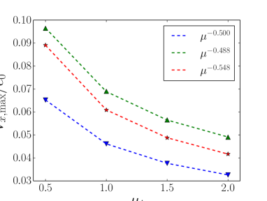
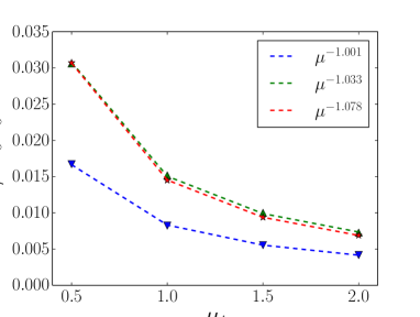
Figure 4: Maximum radial 2-d center-of-mass velocity (left) and average radial acceleration (right) for cold ions (blue), warm ions initialised with zero vorticity (red), and warm ions initialised with non-zero vorticity (green).

Clearly, an inverse dependence of velocities and acceleration on effective ion mass $\mu_{i}$ can be inferred for all cases. For cold ions, the only mass dependence in the present 2-d isothermal gyrofluid model, lies in the gyrofluid polarisation equation, carrying over the mass dependence of the polarisation drift in a fluid model. As deduced from the basic linear considerations in Sec. 3, the maximum blob velocity scales inversely with the square root of the ion species or isotope mass: the plotted fits are close to the expected lines $V_{x,\mathrm{max}}\sim\mu^{-0.5}$.

From dimensional analysis it follows that the acceleration should scale according to $A\sim\gamma^{2}\sigma$, where $\gamma$ is the growth-rate of the linear instability. For $\gamma\sim 1/\sqrt{\mu_{i}}$, we expect $A\sim 1/\mu_{i}$ for cold ions: this is confirmed in Fig. 4 (right) where the fitted exponents are close to $-1$. Warm ion simulations also feature $\mu_{i}$ species mass dependence through the FLR operators $\Gamma_{0}(b)$ and $\Gamma_{1}(b)$, where $b=\rho_{i}^{2}k_{\perp}^{2}=\mu_{i}\tau_{i}\rho_{0}k_{\perp}^{2}$.

We find that for the parameters at hand, the maximum radial velocity for warm ions with zero vorticity initialisation is higher compared to cold ions, with a slightly increased isotopic dependence (seen in an exponent $-0.548$ compared to $-0.500$).

Initialising with non-zero vorticity yields approximately $50\%$ increased velocities compared to cold ions, and slightly weakens the isotopic dependence (expressed by an exponent $-0.488$). This can be attributed to the mass dependence in the FLR operators, which we further discuss below in Sec. 5.0.1.

5 Three-dimensional filament computations

In three dimensions, when the blob extends into an elongated filament along the magnetic field lines, additional physics enters into the model. The basic picture of interchange driving of filaments by charging through $\nabla B$ and curvature drifts to produce a net outward $\mathbf{E}\times\mathbf{B}$ propagation still remains valid. However, the total current continuity balance now also involves parallel currents: $-\nabla\cdot\mathbf{J}_{\mathrm{pol}}=\nabla_{\shortparallel}J_{\shortparallel}+\nabla\cdot\mathbf{J}_{\mathrm{dia}}$.

The detailed balance among the current terms determines the overall motion of the filament. Furthermore, blob filaments in the edge of toroidal magnetised plasmas generally tend to exhibit ballooning in the unfavourable curvature region along the magnetic field. The parallel gradients in a ballooned blob structure also lead to a parallel Boltzmann response, mediated mainly through the resistive coupling of $\nabla_{\shortparallel}(\phi-n_{\rme})$ to $CJ_{||}$ in eq. (2). This tends towards (more or less phase shifted) alignment between the electric potential and the perturbed density, which strongly depends on the collisionality parameter $C$.

For low collisionality, the electric potential in the blob evolves towards establishment of a Boltzmann relation in phase with the electron density along $\mathbf{B}$, so that $n_{\rme}\sim\exp(-\phi)\sim\phi$. This leads to reduced radial particle transport, and the resulting spatial alignment of the potential with the blob density perturbation produces a rotating vortex along contours of constant density, the so-called Boltzmann spinning [33, 34]. Large collisionality leads to a delay in the build-up of the potential within the blob, so that the radial interchange driving can compete with the parallel evolution, and the perpendicular propagation is similar to the 2-d scenario.

In the following we investigate how 3-d filament dynamics is depending on the ion mass. Clearly, we expect an impact in addition to the 2-d effects found in the previous section, since (i) the parallel ion velocity is inversely dependent on ion mass (but is for any ion species slow compared to the electron velicity), (ii) the sheath boundary coupling constants are mass dependent, and (iii) the basic dependence on the ion mass in the polarisation current will play a more role complicated role compared to the 2-d model.

For our present study we chose the free computational parameters basically identical to the 2-d case above: drift scale $\delta=0.01$, curvature $\omega_{B}=0.05$, blob amplitude $A=1$ and perpendicular blob width $\sigma=10$. The Gaussian width of initial parallel density perturbation is given by $\Delta_{z}=\sqrt{32}$, which represents a slight ballooning with some initial sheath connection:

$$n_{\rme}^{3D}(t=0,x,y,z)=n_{e\perp}\cdot\exp\left[\frac{-(z-z_{0})^{2}}{\Delta^{2}}\right]$$ (17)

where $z_{0}$ is the parallel reference coordinate at the outboard mid-plane and $n_{e\perp}(x,y)$ is the perpendicular Gaussian initial perturbation introduced in Sec. 4. In this section we first focus on zero vorticity initial conditions, non-zero conditions will be discussed further below.

The perpendicular domain size is $L_{x}=L_{y}=128\rho_{s}$ with a grid resolution of $N_{x}=N_{y}=256$. The number of parallel grid points is varied between $N_{z}=8$ and $16$. The filament simulations have been tested for convergence with respect to the number of drift planes up to $N_{z}=32$: $N_{z}=8$ yields qualitatively and quantitatively similar results to $N_{z}=16$. The plots showing colour cross sections throughout this article are taken from simulations with $N_{z}=8$, and the presented quantitative results have been obtained for $N_{z}=16$.

We here set $\widehat{\beta}=0$ as electromagnetic effects in the SOL are thought to be of minor importance for the present discussion [30]. The collisionality parameter is chosen in $C=0.5-100$ to cover a likely range of tokamak SOL values. Typical values for the collisionality parameter for the SOL in ASDEX Upgrade L-mode plasmas have in the literature [30] been reported as $C\sim 1-100$, and a reference characteristic collisionality in Ref. [35] for MAST has been given as $C\sim 2$.

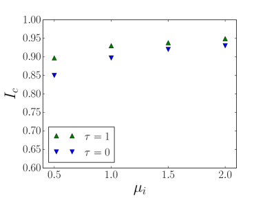
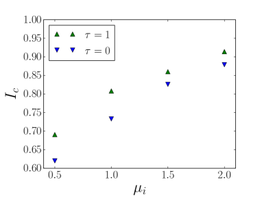
Figure 5: Cross section of 3-d filament at outboard-midplane location ($z=z_{0}$): electron density contour plot at $t=6$ for warm deuterium ions ($\tau_{i}=1$). Boltzmann spinning is dominant for intermediate collisionality parameter ($C=10$, left), and reduced for increased collisionality ($C=100$, right).

Fig. 5 illustrates the dependence of filament evolution with respect to collisionality dependent Boltzmann spinning for warm deuterium ions. The case with $C=10$ represents the strong Boltzmann spinning (drift wave) regime, where density and potential perturbations are closely aligned and the radial filament motion is strongly impeded. Increasing the collisionality to $C=100$ reduces parallel electron dynamics and so effectively increases the lag of potential build-up within the density blob perturbations, so that the Boltzmann spinning is reduced. The substantial perpendicular motion component is in this case partly caused by FLR effects like in the corresponding 2-d case for $\tau_{i}=1$. The $\tau_{i}$ contribution to the ion diamagnetic curvature term results in enhanced radial driving of the blob compared to cold ion cases.

A measure for blob compactness can be introduced [13] by

$$I_{c}(t)=\frac{\int\rmd x\int\rmd yn_{\rme}(x,y,t)h(x,y,t)}{\int\rmd x\int\rmd yn_{\rme}(x,y,t=0)h(x,y,t=0)},$$ (18)

where the Heavyside function $h(x,y,t)$ is defined as

$$h(x,y,t)=1~{}\quad\mathrm{if}~{}(x-x_{\mathrm{max}}(t))^{2}+(y-y_{\mathrm{max}}(t))^{2}<\sigma^{2},$$ (19)

and zero elsewhere. That is, the integral takes non-zero values for density contributions located inside a circle of radius $\sigma$ around its maximum. Fig. 6 quantifies the above observations. In the strong Boltzmann spinning regime ($C=10$, left) the blob retains much of its initial shape, so that the compactness is higher compared to the weak Boltzmann spinning regime ($C=100$, right), where filaments feature a more bean-shaped structure which reduces the compactness measure. At the time of measurement ($t=5$), the heavier isotopic blobs show slightly more compactness, which is an indirect result of decreased velocity: at a given time, the lighter isotopic blobs are further developed and thus less circular. The observed trends are similar for cold ($\tau_{i}=0$) and warm ($\tau_{i}=1$) ions.

For increased collisionality, the deviation from circularity is more pronounced, as the mushroom-cape shape is realized. Blobs in light isotopic plasmas are then again further developed, i.e. finer scales have emerged at the time of recording, resulting in a sharper mass dependence of blob compactness compared to $C=10$, where smaller scales are less prominent.

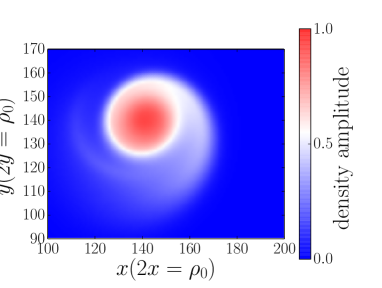
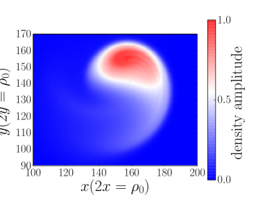
Figure 6: Blob compactness at $t=5$ analysed at the outboard midplane ($z=z_{0}$): strong Boltzmann spinning ($C=10$, left) and weak spinning ($C=100$, right).

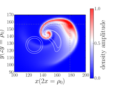
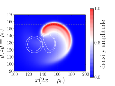
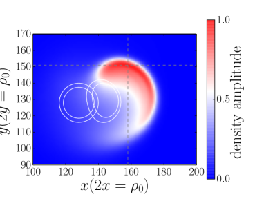
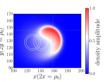
Figure 7: Density contour plots of cold ion blob propagation for different plasma species and $C=100$. White contours depict the initial state ($t=0$) and a subsequent snapshot at $t=4$. The color plot shows the outboard midplane ($z=z_{0}$) electron density perturbation at $t=8$. Shown are protium (top left), deuterium (top right), tritium (bottom left) and singly charged helium-4 (bottom right). The dotted lines give the $x-y$ coordinates of the density maximum.

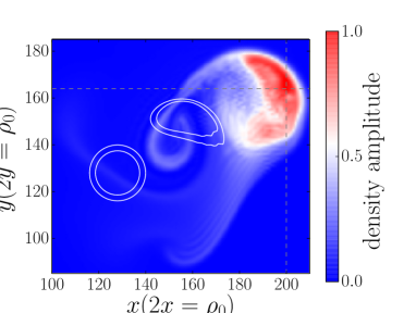
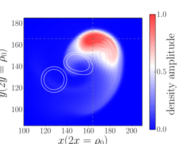
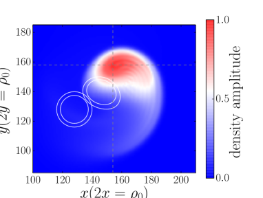
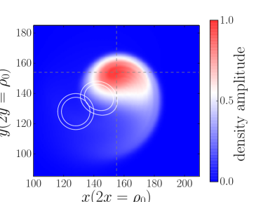
Figure 8: Density contour plots of warm ion blob propagation for different plasma species and $C=100$. White contours depict the initial state ($t=0$) and a subsequent snapshot at $t=4$. The colour plot shows the outboard midplane ($z=z_{0}$) electron density field at $t=8$. Shown are protium (top left), deuterium (top right), tritium (bottom left) and singly charged helium-4 (bottom right). The dotted lines give the $x-y$ coordinates of the density maximum.

Fig. 7 shows filament propagation for cold ions ($\tau_{i}=0$) and weak Boltzmann spinning. This can be compared to Fig. 8 which shows propagation for warm ions ($\tau_{i}=1$) and also weak Boltzmann spinning. It is observed that there is poloidal propagation also for the cold ion case, which is a consequence of the non-vanishing Boltzmann spinning that is also present, although greatly reduced, for these high collisionality ($C=100$) cases. The resulting maximum radial center-of-mass velocites at the outboard midplane ($z=z_{0}$) are shown in Fig. 9 for weak (right) and strong (left) Boltzmann spinning.

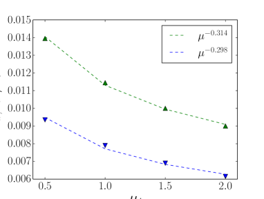
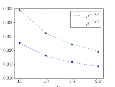
Figure 9: Maximum radial center-of-mass velocities for strong Boltzmann spinning ($C=10$, left) and reduced spinning ($C=100$, right) for cold (blue) and warm ions (green), using zero vorticity initialisation.

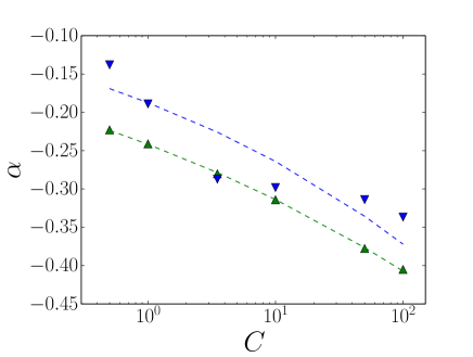
Figure 10: Maximum radial velocity scaling exponents $\alpha$ (analysed at $z=z_{0}$) as a function of the collisionality parameter $C$ for cold (blue) and warm ions (green). The scaling exponents with respect to collisionality are $\alpha\sim C^{0.15}$ (cold ions) and $\alpha\sim C^{0.11}$ (warm ions).

The fits of the exponent in $\mu^{\alpha}$ to the simulation data in Fig. 9 carry evidence that the additional mass dependences introduced by the 3-d model via parallel sheath-boundary conditions and parallel ion velocity dynamics causes the clear deviation from a $1/\sqrt{\mu_{i}}$ scaling.

For high collisionality (and thus reduced Boltzmann spinning), the parallel current is impeded and the dynamics is more two-dimensional than for lower collisionalities. The competing nature of the parallel divergence versus current continuity via the divergence of the polarisation current with collisionality is shown in Fig. 10: for each value of collisionality $C$ we compute the isotopic dependence of the outboard-midplane maximum center-of-mass radial velocity,

$$V_{\mathrm{max}}\sim\mu_{i}^{\alpha(\mu_{i})},$$ (20)

contained in the scaling exponent, $\alpha(\mu_{i})$. For large values of $C$ the resulting dynamics strongly features 2-d propagation characteristics, since the diamagnetic current is almost exclusively closed via the polarisation current, which gives the $1/\sqrt{\mu_{i}}$ scaling introduced in sec. 4. Note that the scaling with respect to $C$ cannot be inferred from linear models.

5.0.1 Non-zero gyrofluid vorticity initialisation

So far we have in this section applied the initial condition $n_{\rme}\equiv\Gamma_{1}n_{i}$ associated with zero initial vorticity. Now the case for non-zero initial vorticity by the condition $n_{\rme}=n_{i}$ is considered.

Fig. 11 shows results for warm ion ($\tau_{i}=1$) computations in the strong ($C=10$, blue) and weak ($C=100$, green) Boltzmann spinning regimes. (Recall that for $\tau_{i}=0$ this discussion is redundant since $\Gamma_{1}(\tau_{i}=0)=1$.) The left figure depicts the maximum radial center-of-mass velocity, and the right figure shows the corresponding average acceleration.

Comparing with Fig. 9 we notice that the resulting filament velocities are similar to those obtained from zero initial vorticity. We also find that the isotopic dependence $\sim\mu_{i}^{\alpha}$ is not significantly altered.

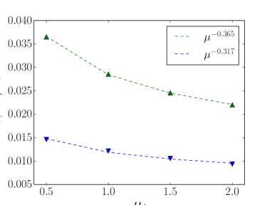
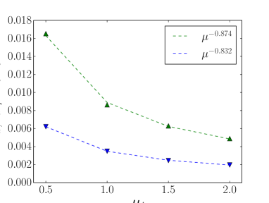
Figure 11: Maximum radial center-of-mass velocity (left) and radial acceleration (right) at $z=z_{0}$ for 3-d warm ion blobs, using non-zero vorticity initialisation at each drift plane, for $C=10$ (blue) and $C=100$ (green).

Recalling the results from 2-d computation in sec. 4, we may conclude that the initialisation is not that important for 3-d numerical simulations with respect to the maximum radial filament velocity. The slight impact of the initial condition on the resulting scaling exponent for the 2-d case may then be connected to the more prominent mass dependence in the polarisation current, which is weakened when parallel currents are taken into account.

5.0.2 Comparison of filaments in deuterium and helium plasmas

When comparing blob filament propagation in deuterium and in fully ionised helium-4 plasmas in the present model, the dynamical evolution is identical in the cold ion limit: in the model parameter $\mu_{i}=m_{i}/(Z_{i}m_{D})$ the doubled mass of the helium nucleus excactly cancels with the doubled positive charge, $Z_{\mathrm{He}}=2$.

Differences are only appearing in warm ion cases. The normalised mass ratio is now identical for both species, $\mu_{\mathrm{D}}=\mu_{\mathrm{He}}=1$. The only model parameter that is different, is the helium temperature ratio, $\tau_{\mathrm{He}}=T_{\mathrm{He}}/Z_{\mathrm{He}}T_{\rme}$. The species mass effects thus appears in the combined $b\sim\mu_{i}\tau_{i}$. In the following we consider plasmas at equal temperature, $T_{\mathrm{D}}=T_{\mathrm{He}}=2T_{\rme}$ such that $\tau_{\mathrm{D}}=2$ and $\tau_{\mathrm{He}}=1$.

The higher charge state of the helium nucleus is also indirectly evident in the reduced electron-ion collision frequency contained in the $C$ -parameter. For electron-ion collisions where the ions are in charge state $Z_{i}$ we have $C\sim\alpha_{e}\nu_{\rme}$, with [36]

$$\alpha_{e}\approx\frac{1+1.198Z_{i}+0.222Z_{i}^{2}}{1+2.966Z_{i}+0.753Z_{i}^{2}}.$$ (21)

For $Z_{i}=1$ we have $\alpha_{e}\approx 0.51$ and $Z_{i}=2$ gives $\alpha_{e}\approx 0.43$.

To account for this dependence, we in the following consider two cases: (1) equal non-normalised collision frequencies, i.e. $C\rightarrow 0.51C$ for deuterium and $C\rightarrow 0.43C$ for helium; (2) using the same $C$ for both deuterium and helium computations.

In case (2), setting first the normalised collisionality parameter $C=10$ identical for both D and He computations results in $V_{\mathrm{D}}=1.41\delta c_{s0}$ and $V_{\mathrm{He}}=1.14\delta c_{s0}$. Setting $C=100$ identical for both D and He gives $V_{\mathrm{D}}=3.2\delta c_{s0}$ and $V_{\mathrm{He}}=2.6\delta c_{s0}$, respectively.

For case (1) we set the electron-ion collision frequency equal for both species, so that different $C$ parameters are used according to equation 21: $C_{\mathrm{D}}=10$ corresponds to $C_{\mathrm{He}}=8.43$, and $C_{\mathrm{D}}=100$ to $C_{\mathrm{He}}=84.3$. In these cases, maximal radial He velocities are $V_{\mathrm{He}}(C=10)=1.09\delta c_{s0}$ and $V_{\mathrm{He}}(C=100)=2.46\delta c_{s0}$.

We find that regardless of how the charge state depency for the relative value of the collision parameter is treated, the filaments in deuterium plasmas move faster than in helium plasmas at identical temperature. This is visualized in Fig. 12 showing filament propagation at equal electron-ion collision frequency and electron temperature.

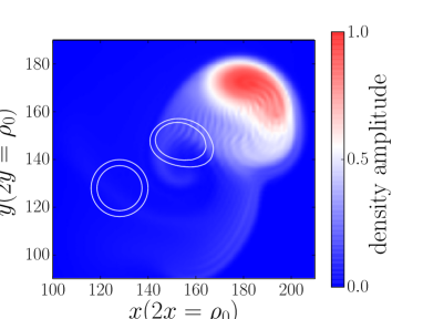
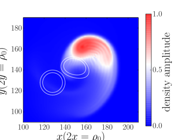
Figure 12: Density contour plots of filament cross sections in deuterium (left) and fully ionised helium-4. White contours depict the initial state ($t=0$) and a subsequent snapshot at $t=4$. The colour plot shows the outboard-midplane ($z=z_{0}$) electron density perturbation field at $t=8$. In both cases $T_{i}=2T_{\rme}$ so that $\tau_{\mathrm{D}}=2$ and $\tau_{\mathrm{He}}=1$. Electron-ion collision frequencies are set equal resulting in $C_{\mathrm{D}}=100$ and $C_{\mathrm{He}}=84.3$.

6 Conclusions

We have investigated filament propagation in SOL conditions characteristic for tokamak fusion devices. Quasi-2-d dynamics is restored in high resistivity regimes, where the maximum radial blob velocity scales inversely proportional with the square root of the ion mass. In 2-d the diamagnetic current drive is closed solely via the polarisation current, yielding this simple characteristic scaling.

The larger inertia through polarisation of more massive ion species effectively slows the evolution of filaments, and the maximum radial velocity occurs later compared to blobs in plasmas with lighter ions.

For non-zero initial vorticity condition, the 2-d warm ion blobs show compact radial propagation, where the isotopic effect through the mass dependent FLR terms is slightly less pronounced.

Boltzmann spinning appears in 3-d situations particularly for low collisionality regimes, and leads to a reduced dependence on the ion isotope mass. The exponent in the scaling $V\sim\mu_{i}^{\alpha}$ has been found to be typically within the range $\alpha\in[-0.1,-0.3]$ for $C<10$, which is a regime relevant for the edge of most present tokamaks.

Considering current continuity, the closure via the parallel current divergence dynamically competes with current loops being closed through the polarisation current. For high collisionalities the parallel current is effectively imepeded and the polarisation current characteristics dominate the blob evolution, producing a more 2-d like velocity dependence with respect to ion mass. The initial condition has been found to have little influence on the maximum radial velocity when in 3-d the parallel closure of the current is taken into account.

For similar ion temperatures and electron-ion collision frequencies, it has been found that helium filaments travel more slowly compared to deuterium filaments in both high and low collisionality regimes.

This work was devoted to the identification of isotopic mass effects on seeded (low amplitude) blob filaments in the tokamak SOL by means of a delta-$f$ gyrofluid model. Naturally, blobs emerge near the separatrix within coupled edge/SOL turbulence. The dependence of fully turbulent SOL transport on the ion mass therefore will have to be further studied within a framework that consistently couples edge and SOL turbulence, preferably through a full-$f$ 3-d gyrofluid (or gyrokinetic) computational model that does not make any smallness assumption on the relative amplitude or perturbations compared to the background [14, 32, 37].

References

References

- [1] Bessenrodt-Weberpals M et al1993, \NF33 1205
- [2] Hawryluk R J 1998, Rev. Mod. Phys. 70 537
- [3] Liu B et al2016, \NF56 056012
- [4] Xu Y et al2013, Phys. Rev. Lett.110 265005
- [5] Boedo J A et al2003, Phys. Plasmas 10 1670
- [6] LaBombard B et al2001, Phys. Plasmas 8 2107
- [7] Theiler C et al2009, Phys. Rev. Lett.103 065001
- [8] D’Ippolito D A, Myra J R and Zweben S J 2011, Phys. Plasmas 18 060501
- [9] Krasheninnikov S I 2001, Phys. Lett. A 283 368
- [10] Krasheninnikov S I, D’Ippolito D A and Myra J R 2008, J. Plasma Phys. 74, 679
- [11] Hahm T S et al2013 \NF53 072002
- [12] Manz P et al2015, Phys. Plasmas 22 022308
- [13] Madsen J et al2011, Phys. Plasmas 18 112504
- [14] Wiesenberger M, Madsen J and Kendl A 2014, Phys. Plasmas 21 092301
- [15] Meyer O H H and Kendl A 2016, Plasma Phys. Control. Fusion58 115008
- [16] Scott B D 2005 Phys. Plasmas 12 102307
- [17] Dorland W et al1993 \PFB 5.3 812–835
- [18] Kendl A and Scott B D 2006 Phys. Plasmas 13 012504
- [19] Kendl A, Scott B D, Ball R and Dewar R L 2003 Phys. Plasmas 10 3684
- [20] Riva F, Lanti E, Jolliet S and Ricci R 2017 Plasmas Phys. Contr. Fusion 59 035001
- [21] Scott B D 1998, Phys. Plasmas 5 2334
- [22] Ribeiro TT and Scott BD 2005 Plasmas Phys. Contr. Fusion 47 1657
- [23] Ribeiro TT and Scott BD 2008 Plasmas Phys. Contr. Fusion 50 055007
- [24] Kendl A 2014 Int. J. Mass Spectrometry 365/366 106–113
- [25] Scott B D 2001, Phys. Plasmas 8 447
- [26] Arakawa A 1966 J. Comput. Phys. 1 119
- [27] Karniadakis G E, Israeli M and Orszag S A 1991 J. Comput. Phys. 97 414
- [28] Naulin V and Nielsen A 2003, J. Sci. Comput. 25 104
- [29] Scott B D 2007, Phys. Plasmas 14 102318
- [30] Manz P et al2013, Phys. Plasmas 20 102307
- [31] Krasheninnikov S I 2001, Phys. Lett. A 283 368
- [32] Held et al\NF2016, 56 126005
- [33] Angus J R et al 2012 Contrib. Plasma Phys. 52 348
- [34] Angus J R and Umansky V M 2014 Phys. Plasmas 21 012514
- [35] Easy L et al2014, Phys. Plasmas 21, 122515
- [36] Hirshman S P 1977, Phys. Fluids 20 589
- [37] Kendl A 2015, Plasma Phys. Control. Fusion57 045012