A continuum model of skeletal muscle tissue with loss of activation

Abstract.

We present a continuum model for the mechanical behavior of the skeletal muscle tissue when its functionality is reduced due to aging. The loss of ability of activating is typical of the geriatric syndrome called sarcopenia. The material is described by a hyperelastic, polyconvex, transverse isotropic strain energy function. The three material parameters appearing in the energy are fitted by least square optimization on experimental data, while incompressibility is assumed through a Lagrange multiplier representing the hydrostatic pressure. The activation of the muscle fibers, which is related to the contraction of the sarcomere, is modeled by the so called active strain approach. The loss of performance of an elder muscle is then obtained by lowering of some percentage the active part of the stress. The model is implemented numerically and the obtained results are discussed and graphically represented.

1. Introduction

Skeletal muscle tissue is one of the main components of the human body, being about 40% of its total mass. Its principal role is the production of force, which supports the body and becomes movement by acting on bones. The mechanism by which a muscle produces force is called activation.

Skeletal muscle tissue is a highly ordered hierarchical structure. The cells of the tissue are the muscular fibers, having a length up to several centimeters; they are organized in fascicles, where every fiber is multiply connected to nerve axons, which drive the activation of the tissue. Connective tissue, which is essentially isotropic, fills the spaces among the fibers. Every fiber contains a concatenation of millions of sarcomeres, which are the fundamental unit of the muscle. With a length of some micrometers, a sarcomere is composed by chains of proteins, mainly actin and myosin, which can slide on each other. This sliding movement produces the contraction of the sarcomere and, ultimately, the contraction of the whole muscle and the production of force and movement.

The aim of this Chapter is to propose a mathematical model of skeletal muscle tissue with a reduced activation, which is typical of a geriatric syndrome named sarcopenia [16]. About thirty years ago, the term sarcopenia (from Greek sarx or flesh and penia or loss) has been introduced in order to describe the age-related decrease of muscle mass and performance. Sarcopenia has since then been defined as the loss of skeletal muscle mass and strength that occurs with advancing age, which in turn affects balance, gait and overall ability to perform even the simple tasks of daily living such as rising from a chair or climbing steps. According to [6], sarcopenia affects more than 50 millions people today and it will affect more than 200 millions in the next 40 years. There is still no generally accepted test for its diagnosis and many efforts are made nowadays by the medical community to better understand this syndrome. Therefore it is desirable to build a mathematical model of muscle tissue affected by sarcopenia. However, to the best of our knowledge, in the biomathematical literature the topic of loss of activation has never been addressed.

In order to use the valuable tools of Continuum Mechanics, during the last decades the skeletal muscle tissue has been often modeled as a continuum material [7, 11, 4, 5], which is usually assumed to be transversely isotropic and incompressible. The former assumption is motivated by the alignment of the muscular fibers, while the latter is ensured by the high water content of the tissue (about 75% of the total volume). Moreover, in view of some experimental tests, the material is assumed to be nonlinear and viscoelastic. Focusing our attention only on the steady properties of the tissue, here we neglect the viscous effects and we set in the framework of hyperelasticity.

In the model that we propose, there are three constitutive prescriptions: one for the hyperelastic energy when the tissue is not active (passive energy), one for the activation and one for the loss of performance. As far as the passive part is concerned, we assume an exponential stress response of the material, which is customary in biological tissues. The particular form that we choose, being a slight simplification of the one proposed in [7], has the advantage of being polyconvex and coercive, giving mathematical soundness to the model and stability to the numerical simulations.

A recent and very promising way to describe the activation is the active strain approach, where the extra energy produced by the activation mechanism is encoded in a multiplicative decomposition of the deformation gradient in an elastic and an active part (see Section 2.2). Unlike the classical active stress approach, in which the active part of the stress is modeled in a pure phenomenological way and a new term has to be added to the passive energy, the active strain method does not change the form of the elastic energy, keeping in particular all its mathematical properties. Moreover, at least in the case of skeletal muscles, the active strain approach seems to be more adherent to the physiology of the tissue, in the sense that at the molecular level the production of force is actually given by a deformation of the material, thanks to the contraction of the sarcomeres. The active part of the deformation gradient is a mathematical representation of such a contraction. The multiplicative decomposition of the deformation gradient has been applied to an active striated muscle in [18, 12]. However, this decomposition involves only a part of the whole elastic energy, which is written as the sum of two terms for the case of a fiber-reinforced material. As far as we know, the active strain approach has never been previously applied to the whole elastic energy of a skeletal muscle tissue. As a drawback, the active strain approach can be a source of some technical difficulties; for instance, in our case fitting the model on the experimental data is not so simple, see eq. (13).

Furthermore, we consider the loss of performance, which is one of the novelties of our model. Unfortunately, there are no experimental data on the elastic properties of a sarcopenic muscle tissue, at least to our knowledge; hence we adopt the naive strategy of reducing the active part of the stress (which is the difference between the stress of the material with and without activation) by a given percentage, represented by the damage parameter $d$ (see Section 3.2). In this way, there is a single parameter in the model which concisely accounts for any effect of the disease.

The proposed model can be numerically implemented using finite element methods. In Section 4 we present some results obtained using FEniCS, an open source collection of Python libraries. Actually, we consider a cylindrical geometry with radial symmetry, so that the numerical domain is two-dimensional and the computational cost is reduced. As far as the boundary conditions are concerned, we prescribe the displacement on the bases of the cylinder and let the lateral surface traction-free. Such simulations show that the experimental results of [10] on the passive and active stress-strain healthy curves, obtained in vivo from a tetanized tibialis anterior of a rat, can be well reproduced by our model. Further, the behavior of the tissue when $d$ increases is analyzed. An ongoing task is to perform a finite element implementation of the model when generic loads are applied, and to consider a realistic three-dimensional muscle mesh. We are now developing a truly hyperelastic model, where the expression of the stress takes into account also the dependence of the activation on the deformation gradient. Actually, in this chapter the stress is computed as the derivative of the hyperelastic energy keeping the active part of the deformation gradient fixed.

In the future, it will be very interesting to find some connections between the damage percentage (the parameter $d$) and other physiological quantities, such as the mass of the muscular tissue or the neuronal activity. Another important topic will be the application of some homogenization techniques in order to deduce an improved constitutive equation for the skeletal muscle starting from its microstructure.

2. Constitutive model

Skeletal muscle tissue is characterized by densely packed muscle fibers, which are arranged in fascicles. Filling the spaces between the fibers and fascicles, connective tissue surrounds the muscle and it is responsible of the elastic recoil of the muscle to elongation. Besides a large amount of water, the fibers themselves contain titin, actin and myosin filaments. The latter two sliding elements form the actual contractile component of the muscle, which is called sarcomere. Since the fibers locally follow a predominant unidirectional alignment, transverse isotropy with respect to that main direction can be assumed. We hence begin by modelling the skeletal muscle tissue as a transversely isotropic nonlinear hyperelastic material with principal direction $\bf m$, which follows the alignment of the muscle fibers.

2.1. Passive model

Let $\bf F$ denote the deformation gradient tensor, $\mathbf{C}=\bf F^{T}\bf F$ the right Cauchy-Green tensor and $\bf M=\bf m\otimes\bf m$ the so called structural tensor. If $\Omega$ denotes the reference configuration occupied by the muscle, we describe its passive behavior by choosing a hyperelastic strain energy function

$$\int_{\Omega}W({\mathbf{C}})dV,$$

where the strain energy density is of the form

(1) $$W({\mathbf{C}})=\frac{\mu}{4}\left\{\frac{1}{\alpha}\left[e^{\alpha(I_{p}-1)}-1\right]+K_{p}-1\right\},$$

with

$$I_{p}=\frac{w_{0}}{3}\operatorname{tr}({\mathbf{C}})+(1-w_{0})\operatorname{tr}({\mathbf{C}}{\bf M}),\ \ K_{p}=\frac{w_{0}}{3}\operatorname{tr}({{\mathbf{C}}^{-1}})+(1-w_{0})\operatorname{tr}({\mathbf{C}}^{-1}\bf M).$$

Here $\mu$ is an elastic parameter and $\alpha$ and $w_{0}$ are positive dimensionless material parameters. The generalized invariants $I_{p}$ and $K_{p}$ are given by a weighted combination of the isotropic and anisotropic components; in particular, $w_{0}$ measures the ratio of isotropic tissue constituents and $1-w_{0}$ that of muscle fibers. Moreover, the term $\operatorname{tr}({\mathbf{C}\bf M})$ represents the squared stretch in the direction of the muscle fiber and is thus associated with longitudinal fiber properties, while the term $\operatorname{tr}({{\mathbf{C}}^{-1}\bf M})$ describes the change of the squared cross-sectional area of a surface element which is normal to the direction $\bf m$ in the reference configuration and thus relates to the transverse behavior of the material [20, 9] (see Fig. 2).

One of the mathematical features of the energy density (1) is that it is polyconvex and coercive [8, 20], hence the equilibrium problem with mixed boundary conditions is well posed.

We remark that ${\mathbf{C}}$ is the identity tensor ${\bf I}$ in the reference configuration, so that $I_{p}=K_{p}=1$, i.e. we have the energy- and stress-free state of the passive muscle tissue (see [8]).

The high content of water is responsible of the nearly incompressible behavior which is experimentally reported for muscle fibers, so that we can assume

(2) $$\det{\mathbf{C}}=1.$$

As is customary in hyperelasticity, the first Piola-Kirchhoff stress tensor, known as nominal stress tensor, can be directly computed by differentiating the strain energy function:

$${\bf P} = \frac{\partial W}{\partial{\bf F}}-p{\bf F}^{-T}=2{\bf F}\frac{\partial W}{\partial{\mathbf{C}}}-p{\bf F}^{-T}=$$

$$= \frac{\mu}{2}{\bf F}\left\{e^{\alpha(I_{p}-1)}\left[\frac{w_{0}}{3}{\bf I}+(1-w_{0}){\bf M}\right]-{\mathbf{C}}^{-1}\left[\frac{w_{0}}{3}{\bf I}+(1-w_{0}){\bf M}\right]{\mathbf{C}}^{-1}\right\}-p{\bf F}^{-T},$$

where $p$ is a Lagrange multiplier associated with the hydrostatic pressure which results from the incompressibility constraint (2).

The material parameters of the model can be obtained from real data. More precisely, concerning the elastic parameter $\mu$, we use the value given in [7], while the other two parameters have been obtained by least squares optimization using the experimental data by Hawkins and Bey [10] about the stretch response of a tetanized tibialis anterior of a rat (see Fig. 1). In Table 1 we furnish the values of the parameters.

$\mu$ [kPa]	$\alpha$ [-]	$w_{0}$ [-]
0.1599	19.35	0.7335

Table 1. Material parameters of the passive model.

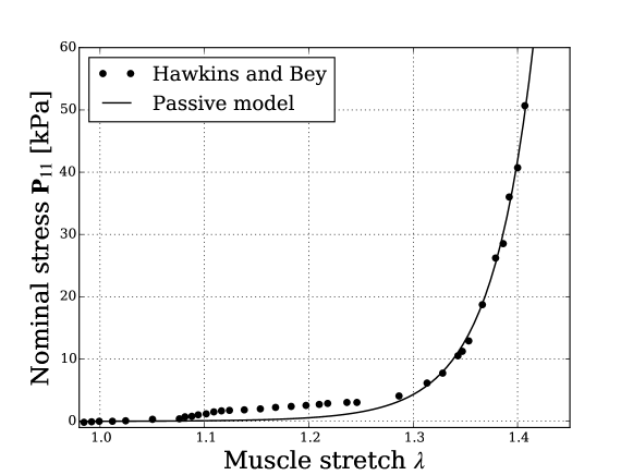
Figure 1. Comparison of the passive model in uniaxial tension with the experimental data of a rat tibialis anterior muscle reported in [10].

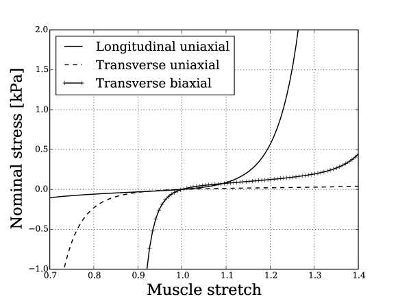
Figure 2. Transversely isotropic behavior of the model.

We remark that the strain energy function (1) is a slight simplification of the one proposed by Ehret, Böl and Itskov in [7]:

(4) $$W_{\text{EBI}}(\mathbf{C})=\frac{\mu}{4}\left\{\frac{1}{\alpha}\left[e^{\alpha(I_{p}-1)}-1\right]+\frac{1}{\beta}\left[e^{\beta(K_{p}-1)}-1\right]\right\},$$

where $\alpha=19.69,\beta=1.190,w_{0}=0.7388$. Actually, our simplification consists in linearizing the term related to $K_{p}$, which describes the transverse behavior. This is motivated by the fact that the parameter $\beta$ is much smaller than $\alpha$. In Fig. 3 we can see the comparison between the nominal stress in the direction of the stretch of the two models when the muscle fibers are elongated in their direction.

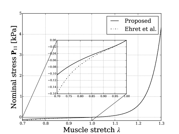
Figure 3. Comparison between the passive stress here proposed and the one studied in [7] during uniaxial tension along the fibers.

2.2. Active model

One of the main features of the skeletal muscle tissue is its ability of being voluntarily activated. Skeletal muscles are activated through electrical impulses from motor nerves; the activation triggers a chemical reaction between the actin and myosin filaments which produces a sliding of the molecular chains, causing a contraction of the muscle fibers.

During the last decades, many authors tried to mathematically model the process of activation, mainly with two different approaches (for a review see [2]). The most famous approach followed in the literature is called active stress and it consists in adding an extra term to the stress, which accounts for the contribution given by the activation (see for example [15, 3, 11]). However, this is an ad hoc method, usually not related to the sliding movement of the filaments in the sarcomeres, which is the main mechanism of contraction at the mesoscale.

More recently, the active strain approach was proposed by Taber and Perucchio [21] in order to describe the activation of the cardiac tissue, following previous theories of growth and morphogenesis, as well as several models of plasticity. The method for soft living tissues is explained in [17]. Differently from the active stress approach, this method does not change the form of the strain energy function; rather, it assumes that only a part of the deformation gradient, obtained by a multiplicative decomposition, is responsible for the store of elastic energy. This method is related to the biological meaning of activation and can be reasonably adopted also in our case. To the best of our knowledge, the active strain approach has never been followed for the skeletal muscle tissue in literature.

We begin by rewriting the deformation gradient as ${\bf F}={\bf F}_{e}{\bf F}_{a}$, where ${\bf F}_{e}$ is the elastic part and ${\bf F}_{a}$ describes the active contribution (see Fig. 4).

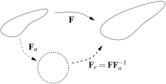
Figure 4. Pictorial view of the active strain approach.

The active strain ${\bf F}_{a}$ represents a change of the reference volume elements due to the contraction of the sarcomeres, so that it does not contribute to the elastic energy. A reference volume element, distorted by ${\bf F}_{a}$, needs a further deformation ${\bf F}_{e}$ to match the actual volume element, which accommodates both the external forces and the active contraction. Notice that neither ${\bf F}_{a}$ nor ${\bf F}_{e}$ need to be the gradients of some displacement, that is, it is not necessary that they fulfill the compatibility condition $\operatorname{curl}{\bf F}_{a}=0$ or $\operatorname{curl}{\bf F}_{e}=0$.

The volume elements are modified by the internal active forces without changing the elastic energy, hence the strain energy function of the activated material has to be computed using ${\mathbf{C}}_{e}={\bf F}_{e}^{T}{\bf F}_{e}$ and taking into account ${\bf F}_{e}={\bf F}{\bf F}_{a}^{-1}$. If ${\bf F}_{a}=\mbox{grad}\chi_{a}$ for some displacement $\chi_{a}$, then from Fig. 4 by a change of variables it is easy to see that

$$\int_{\chi_{a}(\Omega)}W({\mathbf{C}}_{e})d\widehat{V}=\int_{\Omega}W({\bf F}^{-T}_{a}{\mathbf{C}}{\bf F}_{a}^{-1})(\det{\bf F}_{a})d{V}.$$

The right-hand side of the previous equation is well defined also when ${\bf F}_{a}$ does not come from a global displacement, and it describes the strain energy of the active body. We then obtain the modified hyperelastic energy density

$$\widehat{W}({\mathbf{C}})=(\det{\bf F}_{a})W({\mathbf{C}}_{e})=(\det{\bf F}_{a})W({\bf F}^{-T}_{a}{\mathbf{C}}{\bf F}_{a}^{-1}).$$

We now have to model the active part ${\bf F}_{a}$. Since the activation of the muscle consists in a contraction along the fibers, we choose

(5) $${\bf F}_{a}={\bf I}-\gamma{\bf m}\otimes{\bf m},$$

where $0\leq\gamma<1$ is a dimensionless parameter representing the relative contraction of activated fibers ($\gamma=0$ meaning no activation). Then the modified strain energy density becomes

(6) $$\widehat{W}({\mathbf{C}})=(1-\gamma)W({\mathbf{C}}_{e})=(1-\gamma)\frac{\mu}{4}\left\{\frac{1}{\alpha}\left[e^{\alpha(I_{e}-1)}-1\right]+K_{e}-1\right\},$$

$$I_{e}=\frac{w_{0}}{3}\operatorname{tr}({\mathbf{C}}_{e})+(1-w_{0})\operatorname{tr}({\mathbf{C}}_{e}{\bf M}),\ \ K_{e}=\frac{w_{0}}{3}\operatorname{tr}({{{\mathbf{C}}_{e}}^{-1}})+(1-w_{0})\operatorname{tr}({{\mathbf{C}}_{e}}^{-1}{\bf M}).$$

The corresponding first Piola-Kirchhoff stress tensor is given by

(7) $$\widehat{\bf P}= \det{\bf F}_{a}\frac{\partial W}{\partial{\bf F}_{e}}{\bf F}_{a}^{-1}-\widehat{p}{\bf F}^{-T}=$$

$$= \frac{\mu}{2}(1-\gamma){\bf F}_{e}\left\{e^{\alpha(I_{e}-1)}\left[\frac{w_{0}}{3}{\bf I}+(1-w_{0}){\bf M}\right]-{\mathbf{C}}_{e}^{-1}\left[\frac{w_{0}}{3}{\bf I}+(1-w_{0}){\bf M}\right]{\mathbf{C}}_{e}^{-1}\right\}{\bf F}_{a}^{-1}$$

$$-\widehat{p}{\bf F}^{-T},$$

where $\widehat{p}$ accounts for the incompressibility constraint $\det\mathbf{C}=1$. Notice that, since the activation (5) does not preserve volume and the material has to be globally incompressible, one has that $\det{\mathbf{C}}_{e}\neq 1$, so that the material is elastically compressible. As far as the strain energy density is concerned, a factor $(1-\gamma)$ appears in (6) which keeps into account the compressibility of ${\bf F}_{a}$. It would be interesting to study also other kinds of passive energies, involving the quantity $\det\mathbf{C}$, in order to better describe the elastic compressibility of the material.

In Fig. 5 we represent, for several values of the parameter $\gamma$, the stress-strain curve for a uniaxial tension along the fibers. If the muscle is activated ($\gamma>0$), then (the absolute value of) the stress increases with $\gamma$ and the value of the stretch such that the stress is zero becomes less than one.

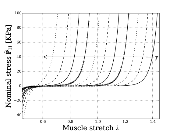
Figure 5. Stress-stretch curves in uniaxial tension for several values of $\gamma$ from $0$ to $0.4$.

3. Modelling the activation on experimental data

The activation parameter $\gamma$, which was assumed constant in the previous section, in fact usually depends on the deformation gradient. In typical experiments on a tetanized skeletal muscle it is apparent that the contraction of the fibers due to activation varies with their stretch, reaching a maximum value and then decreasing. Fig. 6 shows the qualitative relation between the elongation and the developed stress. This section will be devoted to taking into account this phenomenon. Specifically, the expression of $\gamma$ will be determined matching an experiment-based relation between stress and strain with our model (7).

In order to find the relation between stress and strain, the experiments in vivo are usually performed in two steps. First, the stress-strain curve is obtained without any activation (passive curve). Second, by an electrical stimulus the muscle is isometrically kept in a tetanized state and the total stress-strain curve is plotted. The last curve, which is qualitatively represented in Fig. 6, depends on the reciprocal position of actin and myosin chains. By taking the difference of the two curves one can obtain the active curve, describing the amount of stress due to activation. It is useful to find a mathematical expression of such a curve, in order to take into account the experimental behavior of the active contraction. This issue has already been addressed in several papers, see e.g. [7, 11, 22, 23, 13, 3, 4].

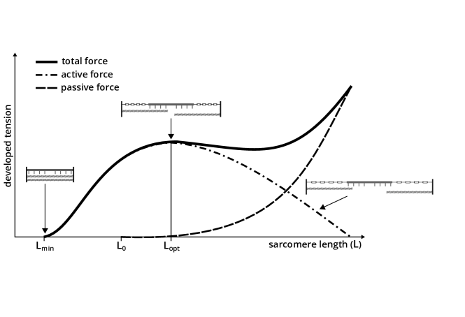
Figure 6. Length-tension relationship of a sarcomere. Here we denote by $\mathsf{L_{opt}}$ the length at which the sarcomere produces the maximum force in isometric experiments, by $\mathsf{L_{0}}$ the rest length and by $\mathsf{L_{min}}$ the minimal length of the sarcomere (fully activated).

Denoting with $\lambda$ the ratio between the current length of the muscle and its original length, we assume the active curve to be of the form

(8) $$P_{act}(\lambda)=\left\{\begin{aligned} &P_{opt}\exp\left[-k\frac{(\lambda^{2}-\lambda_{opt}^{2})^{2}}{\lambda-\lambda_{min}}\right]&\text{if $\lambda>\lambda_{min}$},\\[4.30554pt] &0&\text{otherwise},\end{aligned}\right.$$

where $\lambda_{min}$ is the minimum stretch value after which the activation starts (i.e. the lower bound for the stretch at which the myofilaments begin to overlap) and $k$ is merely a fitting parameter. The coordinates $(\lambda_{opt},P_{opt})$ identify the position of the maximum of the curve. As it is explained in [7], the value of $P_{opt}$ takes into account some information at the mesoscale level, such as the number of activated motor units and the interstimulus interval; according to the literature [7, 11], it is set at $P_{opt}=73.52$ kPa. The numerical values of the other three parameters, deduced through least squares optimization on the data reported in [10], are given in Table 2.

Table 2. Material parameters of the active model.

$\lambda_{min}$ [-]	$\lambda_{opt}$ [-]	$k$ [-]	$P_{opt}$ [kPa]
0.6243	1.1704	0.4342	73.52

The expression (8) has the advantage of describing the asymmetry between the ascending and descending branches of the active curve obtained in [10]. Indeed, even if the asymmetry is not so evident in their curve, due to the fact that there are only few data on the descending branch, it is a typical feature of several experimentally measured sarcomere length-force relation. Moreover, as one can easily see in Fig. 7, the convex behavior of the data nearby $\lambda_{min}$ is well fitted.

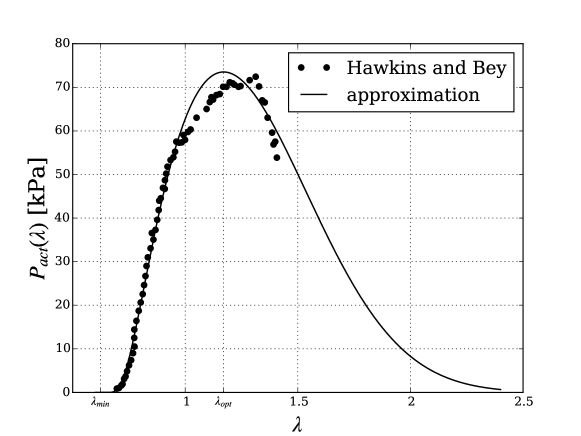
Figure 7. Plot of the active curve (8) with the parameters reported in Table 2 together with the representation of the experimental data given in [10].

3.1. The activation parameter $\gamma$ as a function of the elongation

Now our aim is to obtain $P_{act}(\lambda)$ given in (8) from the model described in Section 2.2. In order to reach our purpose, we have to model the activation parameter $\gamma$ as a function of the stretch.

As in the experiments of Hawkins and Bey [10], let us consider a uniaxial simple tension along the fibers. For simplicity, we assume that the fibers follow the direction ${\bf m}={\bf e}_{1}$. Since the skeletal muscle tissue is modeled as an incompressible transversely isotropic material, the general form of the deformation gradient ${\bf F}$ is given by

$${\bf F}=\begin{pmatrix}\lambda&0&0\\ 0&\frac{1}{\sqrt{\lambda}}&0\\ 0&0&\frac{1}{\sqrt{\lambda}}\end{pmatrix}.$$

Then using the notation introduced in Section 2.2, one has

$${\mathbf{C}}_{e} =\begin{pmatrix}\frac{\lambda^{2}}{(1-\gamma)^{2}}&0&0\\ 0&\frac{1}{\lambda}&0\\ 0&0&\frac{1}{\lambda}\end{pmatrix},$$

$$I_{e} =\frac{w_{0}}{3}\left[\frac{\lambda^{2}}{(1-\gamma)^{2}}+\frac{2}{\lambda}\right]+(1-w_{0})\frac{\lambda^{2}}{(1-\gamma)^{2}},$$

$$K_{e} =\frac{w_{0}}{3}\left[\frac{(1-\gamma)^{2}}{\lambda^{2}}+2\lambda\right]+(1-w_{0})\frac{(1-\gamma)^{2}}{\lambda^{2}}.$$

In this case, it is convenient to look at the strain energy as a function of the stretch $\lambda$ and the activation parameter $\gamma$:

(9) $$\widehat{W}(\lambda,\gamma)=(1-\gamma)W(\lambda,\gamma)=(1-\gamma)\frac{\mu}{4}\left\{\frac{1}{\alpha}\left[e^{\alpha(I_{e}-1)}-1\right]+K_{e}-1\right\}.$$

Then the nominal stress along the fiber direction is given by

(10) $$P_{tot}(\lambda,\gamma):=\frac{\partial\widehat{W}}{\partial\lambda}=(1-\gamma)\frac{\mu}{4}\left[I_{e}^{\prime}e^{\alpha(I_{e}-1)}+K_{e}^{\prime}\right],$$

where

$$I_{e}^{\prime} =\frac{\partial I_{e}}{\partial\lambda}=2\frac{w_{0}}{3}\left[\frac{\lambda}{(1-\gamma)^{2}}-\frac{1}{\lambda^{2}}\right]+2(1-w_{0})\frac{\lambda}{(1-\gamma)^{2}},$$

$$K_{e}^{\prime} =\frac{\partial K_{e}}{\partial\lambda}=2\frac{w_{0}}{3}\left[-\frac{(1-\gamma)^{2}}{\lambda^{3}}+1\right]-2(1-w_{0})\frac{(1-\gamma)^{2}}{\lambda^{3}}.$$

We can get the passive stress by setting $\gamma=0$:

(11) $$P_{pas}(\lambda):=P_{tot}(\lambda,0)= \dfrac{\mu}{2} \left\{\left[\left(1-\frac{2}{3}w_{0}\right)\lambda-\frac{w_{0}}{3}\frac{1}{\lambda^{2}}\right]e^{\alpha\left[\left(1-\frac{2}{3}w_{0}\right)\lambda^{2}+\frac{w_{0}}{3}\frac{2}{\lambda}-1\right]}\right.$$

$$- \left.\left(1-\frac{2}{3}w_{0}\right)\frac{1}{\lambda^{3}}+\frac{w_{0}}{3}\right\}.$$

We remark that the values of $P_{tot}$ and $P_{pas}$ can also be obtained by computing the first component of the stress given by (7) and (2.1) after finding the hydrostatic pressure from the conditions $\widehat{P}_{22}=\widehat{P}_{33}={P}_{22}={P}_{33}=0$ (traction-free lateral surface).

Our aim is to find the value of $\gamma$ such that

(12) $${P}_{tot}(\lambda,\gamma)={P}_{act}(\lambda)+{P}_{pas}(\lambda),$$

where ${P}_{act}(\lambda)$ is given by (8). Unfortunately, this leads to an equation for $\gamma$ which cannot be explicitly solved:

$$(1-\gamma)\left\{\left[\left(1-\frac{2}{3}w_{0}\right)\frac{\lambda}{(1-\gamma)^{2}}-\frac{w_{0}}{3}\frac{1}{\lambda^{2}}\right]e^{\alpha\left[\left(1-\frac{2}{3}w_{0}\right)\frac{\lambda^{2}}{(1-\gamma)^{2}}+\frac{w_{0}}{3}\frac{2}{\lambda}-1\right]}\right.$$

(13) $$\left.+\frac{w_{0}}{3}-\left(1-\frac{2}{3}w_{0}\right)\frac{(1-\gamma)^{2}}{\lambda^{3}}\right\}=\frac{2}{\mu}\left[{P}_{act}(\lambda)+{P}_{pas}(\lambda)\right].$$

However one can employ standard numerical methods and plot the solution. Fig. 8₁, which is obtain by a bisection method, shows $\gamma$ as a function of $\lambda$. We remark that $\gamma$ vanishes before $\lambda_{min}$, indeed in this region there is no difference between total and passive stress. The corresponding behavior of the stresses is plotted in Fig. 8₂, which is very similar to the representative plot of Fig. 6.

We emphasize that the previous model is not strictly hyperelastic, since in the expression of the stress (7) the derivative of $\gamma$ with respect to $\mathbf{F}$ has been neglected. We are now working on a truly hyperelastic model, which can be useful for some numerical implementations.

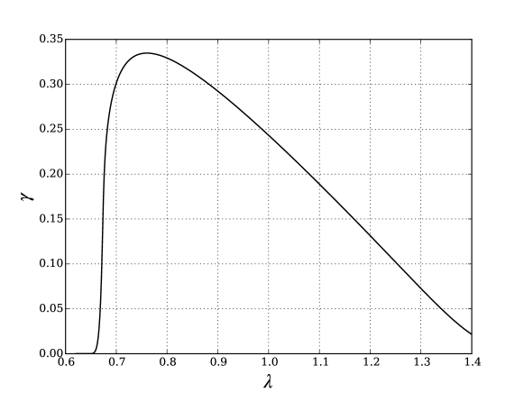
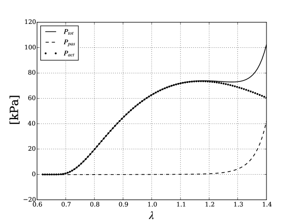
Figure 8. The first figure shows the behavior of $\gamma$ when $\lambda$ varies: the corresponding plots of $P_{tot}$ and $P_{act}$ are given in the second figure, together with $P_{pas}$.

3.2. Loss of activation

We now want to describe from a mathematical point of view the loss of performance of a skeletal muscle tissue. As we have already explained in the Introduction, this is one of the main effects of sarcopenia, which is a typical syndrome of advanced age.

In [14, 24] it is remarked that aging is associated with changes in muscle mass, composition, activation and material properties. In sarcopenic muscle, there is a loss of motor units via denervation and a net conversion in slow fibers, with a resulting loss in muscle power. Hence, the loss of performance of a sarcopenic muscle can be described as a weakening of the activation of the fibers.

Unfortunately, as far as we know, there are no experimental data describing a uniaxial simple tension along the fibers of a sarcopenic muscle. For this reason, we try to describe the loss of activation by a parameter $d$ which lowers the curve $P_{act}(\lambda)$ given by (8). The parameter $d$ describes the percentage of disease or damage: if $d=0$, then the muscle is healthy. In order to get our aim, we multiply the function $P_{act}(\lambda)$ by the factor $1-d$, as one can see in Fig. 9. Notice that such a choice can be overly simple: for instance, it implies that the maximum is always attained at $\lambda_{opt}$, even if there is no experimental evidence of that. However, the presence of $d$ allows to describe, at least qualitatively, the loss of performance of a muscle, which is one of the goals of our model.

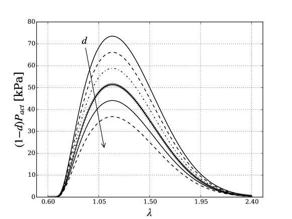
Figure 9. Plot of $(1-d)P_{act}(\lambda)$ vs $\lambda$ when $d$ varies from $0$ to $0.5$.

4. Numerical validation

Finally, we simulate numerically the contraction and the elongation of a slab of skeletal muscle tissue represented by a cylinder. We assume radial symmetry, so that the mesh is a rectangle. The ends of the cylinder are assumed to remain perpendicular to the axial direction. The rectangle is modeled by the hyperelastic model presented in the previous sections. The active contractile fibers are aligned along the length of the rectangle, which coincides with ${\bf e}_{1}$. The passive and active material parameters are given in Tables 1 and 2, respectively. Concerning the boundary conditions, the cylinder is fixed at one end and elongated to a given length, in order to recreate the situation of the experiments reported in [10]. The lateral surface is assumed to be tension-free.

The analysis is performed by using the computing environment FEniCS. The FEniCS Project [1] is a collection of numerical software, supported by a set of novel algorithms and techniques, aimed at the automated solution of differential equations using finite element methods.

As it is explained in Section 3.1, one of the main features of our model is the dependence of the activation parameter $\gamma$ on the stretch $\lambda$. The function $\gamma(\lambda)$ solves the implicit equation (13), which ensures that the corresponding stress curves fit the experimental data. However, even if this equation can be solved using numerical methods, it is interesting to find an explicit function in order to analyze qualitatively the active model and to run the simulations in FEniCS. Moreover, the explicit function $\gamma(\lambda)$ has to be very precise, since a slight error on $\gamma$ deeply affects the behavior of the total stress. Hence, it is reasonable to relate the expression of $\gamma$ to the material parameters and the quantities involved in (13). An idea is to isolate the exponential in (13) and to express its exponent by a first step approximation of a fixed-point method. We then obtain the following expression of $\gamma$:

$$\gamma(\lambda)= \left\{\begin{aligned} &a\left[\sqrt{\frac{1-\frac{2}{3}w_{0}}{\frac{g(\lambda_{min})}{\alpha}+\frac{w_{0}}{3\lambda_{min}}}}\lambda_{min}-\sqrt{\frac{1-\frac{2}{3}w_{0}}{\frac{g(\lambda)}{\alpha}+\frac{w_{0}}{3\lambda}}}\lambda\right]&\text{if $\lambda>\lambda_{min}$},\\[4.30554pt] &0&\text{otherwise},\end{aligned}\right.$$

$$g(\lambda)= \ln\alpha+\alpha\left(1-\frac{w_{0}}{\lambda}\right)-\frac{1}{2}\ln\left(\frac{1-\frac{2}{3}w_{0}}{\frac{1}{\alpha}+\frac{w_{0}}{3\lambda}}\right)$$

$$+\ln\left\{b\frac{2}{\mu}\left[P_{act}(\lambda)+P_{pas}(\lambda)\right]+\sqrt{\frac{1-\frac{2}{3}w_{0}}{\frac{1}{\alpha}+\frac{w_{0}}{3\lambda}}}\left[\frac{\left(1-\frac{2}{3}w_{0}\right)^{2}}{\frac{1}{\alpha}+\frac{w_{0}}{3\lambda}}-\lambda\frac{w_{0}}{3}\right]\right\},$$

where $a$ and $b$ are dimensionless fitting parameters: $a$ is related to the magnitude of $\gamma$, while $b$ acts on the curves (8) and (11), which are the terms of the equation not depending on $\gamma$. Performing a least square optimization on the resulting $P_{act}$, one gets $a=1.0133$ and $b=0.2050$.

Fig. 10 shows the plot of the function $\gamma(\lambda)$ given in (4) in comparison to the numerical solution of equation (13) obtained by a bisection method.

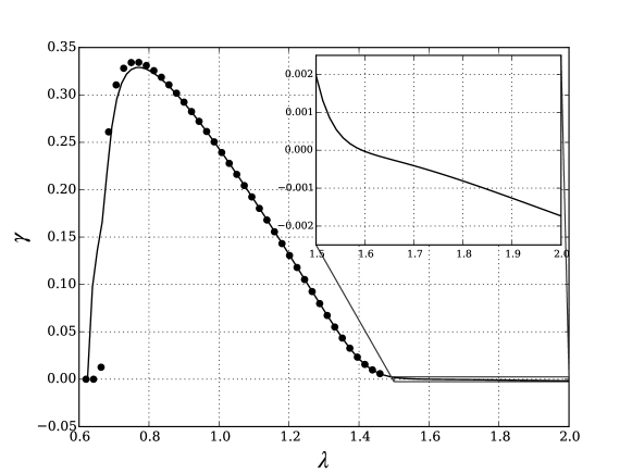
Figure 10. Comparison between the behavior of $\gamma(\lambda)$ in (4) (solid line) and the numerical solution of equation (13) (dotted line).

Notice that the function defined in (4) is continuous; in particular we impose $\gamma(\lambda_{min})=0$, so that the starting value of activation does not change. Moreover, the function approximates very well the numerical values of $\gamma$ in the range $0.7<\lambda<1.5$. However, the fitting is not so good when $\lambda$ becomes larger: for instance, the function is negative for $\lambda\geq 1.6$. Nevertheless, the latter behavior of $\gamma$ does not influence too much the curve $P_{tot}$, since in that region $P_{pas}\gg P_{act}$. Indeed, one can even neglect the activation for large stretches. The total stress response is plotted in Fig. 11 in comparison to the data given in [10].

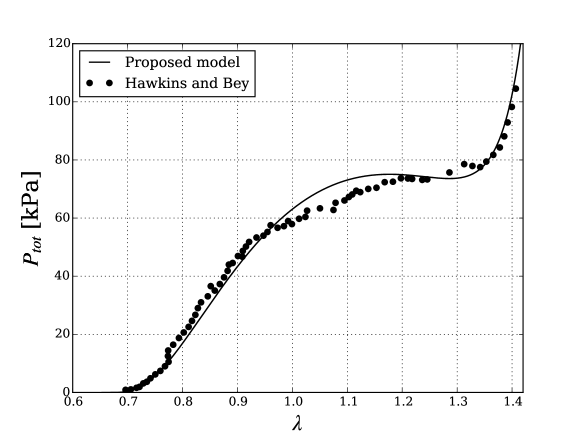
Figure 11. Trend of $P_{tot}$ when $\gamma$ is given by (4) and $\lambda$ varies.

Finally, it is interesting to run the simulations in the case of loss of activation, i.e. when the damage parameter $d$ varies. In order to find the suitable activation function $\gamma(\lambda)$, it is sufficient to multiply the term $P_{act}$ in (4) by $(1-d)$. As one would expect from Fig. 9, we have that when $d$ increases the activation $\gamma$ decreases (Fig. 12₁). This means that lowering the curve of $P_{act}$ results in a decrease of $\gamma(\lambda)$, which leads to a lowered total stress response. As one can see in Fig. 12₂, the damage parameter mainly affects the value of the stress in the region near $\lambda_{opt}$, where the active stress reaches its maximum. However, the qualitative behavior of the stress curve does not change, at least for $d\leq 0.5$. In particular, after a plateau, the stress follows the exponential growth of the passive curve.

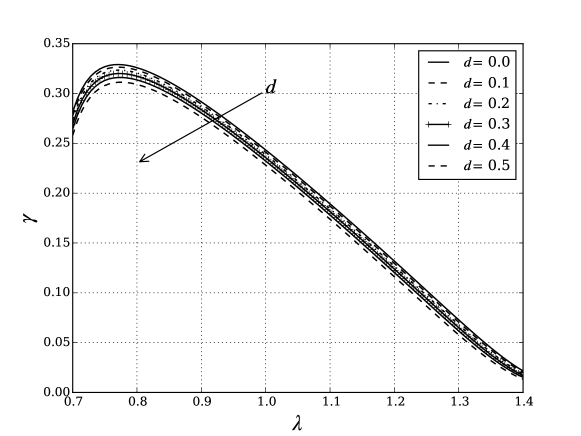
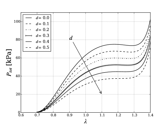
Figure 12. Behavior of $\gamma$ and $P_{tot}$ when $\lambda$ varies.

References

- [1] M. S. Alnæs, J. Blechta, J. Hake, A. Johansson, B. Kehlet, A. Logg, C. Richardson, J. Ring, M. E. Rognes, and G. N. Wells. The FEniCS Project Version 1.5. Archive of Numerical Software, 100:9–23, 2015.
- [2] D. Ambrosi and S. Pezzuto. Active Stress vs. Active Strain in Mechanobiology: Constitutive Issues. Journal of Elasticity, 107:199–212, 2012.
- [3] S. S. Blemker, P. M. Pinsky, and S. L. Delp. A 3D model of muscle reveals the causes of nonuniform strains in the biceps brachii. Journal of Biomechanics, 38:657–665, 2005.
- [4] M. Böl and S. Reese. Micromechanical modelling of skeletal muscles based on the finite element method. Computer Methods in Biomechanics and Biomedical Engineering, 11:489–504, 2008.
- [5] G. Chagnon, M. Rebouah, and D. Favier. Hyperelastic Energy Densities for Soft Biological Tissues: A Review. Journal of Elasticity, 120:129–160, 2015.
- [6] A. J. Cruz-Jentoft, J. P. Baeyens, J. M. Bauer, Y. Boirie, T. Cederholm, F. Landi, F. C. Martin, J. P. Michel, Y. Rolland, S. M. Schneider, E. Topinková, M. Vandewoude, and M. Zamboni. Sarcopenia: European consensus on definition and diagnosis. Age and Ageing, 39:412–423, 2010.
- [7] A. E. Ehret, M. Böl, and M. Itskov. A continuum constitutive model for the active behaviour of skeletal muscle. Journal of the Mechanics and Physics of Solids, 59:625–636, 2011.
- [8] A. E. Ehret and M. Itskov. A polyconvex hyperelastic model for fiber-reinforced materials in application to soft tissues. Journal of Materials Science, 42:8853–8863, 2007.
- [9] A. E. Ehret and M. Itskov. Modeling of anisotropic softening phenomena: Application to soft biological tissues. International Journal of Plasticity, 25:901–919, 2009.
- [10] D. Hawkins and M. Bey. A Comprehensive Approach for Studying Muscle-Tendon Mechanics. ASME Journal of Biomechanical Engineering, 116:51–55, 1994.
- [11] T. Heidlauf and O. Röhrle. A multiscale chemo-electro-mechanical skeletal muscle model to analyze muscle contraction and force generation for different muscle fiber arrangements. Frontiers in Physiology, 5:1–14, 2014.
- [12] B. Hernández-Gascón, J. Grasa, B. Calvo, and J. F. Rodríguez. A 3D electro-mechanical continuum model for simulating skeletal muscle contraction. Journal of Theoretical Biology, 335:108–118, 2013.
- [13] T. Johansson, P. Meier, and R. Blickhan. A Finite-Element Model for the Mechanical Analysis of Skeletal Muscles. Journal of Theoretical Biology, 206:131–149, 2000.
- [14] T. Lang, T. Streeper, P. Cawthon, K. Baldwin, D. R. Taaffe, and T. B. Harris. Sarcopenia: etiology, clinical consequences, intervention, and assessment. Osteoporos Int, 21:543–559, 2010.
- [15] J. A. C. Martins, E. B. Pires, R. Salvado, and P. B. Dinis. A numerical model of passive and active behavior of skeletal muscles. Computer Methods in Applied Mechanics and Engineering, 151:419–433, 1998.
- [16] A. Musesti, G. G. Giusteri, and A. Marzocchi. Predicting Ageing: On the Mathematical Modelization of Ageing Muscle Tissue. In G. Riva et al., editor, Active Ageing and Healthy Living. IOS press, 2014. Chapter 17.
- [17] P. Nardinocchi and L. Teresi. On the Active Response of Soft Living Tissues. Journal of Elasticity, 88:27–39, 2007.
- [18] C. Paetsch, B. A. Trimmer, and A. Dorfmann. A constitutive model for active-passive transition of muscle fibers. International Journal of Non-Linear Mechanics, 47:377–387, 2012.
- [19] G. Riva, P. Ajmone Marsan, and C. Grassi. Active Ageing and Healthy Living. IOS press, 2014.
- [20] J. Schröder and P. Neff. Invariant formulation of hyperelastic transverse isotropy based on polyconvex free energy functions. International Journal of Solids and Structures, 40:401–445, 2003.
- [21] L. A. Taber and R. Perucchio. Modeling Heart Development. Journal of Elasticity, 61:165–197, 2000.
- [22] J. L. van Leeuwen. Optimum power output and structural design of sarcomeres. Journal of Theoretical Biology, 149:229–256, 1991.
- [23] J. L. van Leeuwen. Muscle function in locomotion. In Advances in Comparative and Environmental Physiology. Springer Heidelberg Berlin, 1992. Chapter 7.
- [24] S. von Haehling, J. E. Morley, and S. D. Anker. An overview of sarcopenia: facts and numbers on prevalence and clinical impact. Journal of Cachexia, Sarcopenia and Muscle, 1:129–133, 2010.