Polaron resonances in two vertically stacked quantum dots

Abstract

In this work, we present a theoretical study of polaron states in a double quantum dot system. We present realistic calculations which combine 8 band $\bm{k}\!\cdot\!\bm{p}$ model, configuration interaction approach and collective modes method. We investigate the dependence of polaron energy branches on axial electric field. We show that coupling between carriers and longitudinal optical phonons via Fröhlich interaction leads to qualitative and quantitative reconstruction of the optical spectra. In particular, we study the structure of resonances between the states localized in different dots. We show that $p$-shell states are strongly coupled to the phonon replicas of $s$-shell states, in contrast to the weak direct $s$-$p$ coupling. We discuss also the dependence of the phonon-assisted tunnel coupling strength on the separation between the dots.

I Introduction

Self assembled quantum dots (QDs) are continuously attracting attention both in fundamental research, as well as in the development of novel applications in quantum optics and quantum information. With the continuing effort and progress in miniaturization, QDs find technological use in many types of devices, including QD laserszhuo14 , screens, solar cellsschaller04 and many others.

One of the most interesting aspects of QD physics is related to carrier-phonon coupling. Apart from dissipative processes induced by phonons, this coupling can lead to the formation of polarons, that is, eigenstates of the interacting carrier-phonon systems in which the carrier state is correlated with the coherent field of longitudinal optical (LO) phonons. In QDs, the carrier spectrum is discrete, while the relatively weak carrier localization limits the effectively coupled LO phonons to the nearly dispersionless zone-center part of their spectrum. As a result, the system is in the strong coupling regime and the polaron states are manifested in the form of pronounced resonances whenever one excited state spectrally crosses a LO-phonon replica of another state ham99 ; ham02 ; kaczmarkiewicz10 . The width of the resonances provides a natural quantitative measure of the strength of the carrier-phonon coupling. The effectively dispersionless nature of LO phonons forming the polaron states in QDs makes it possible to describe the system in terms of a finite number of collective modes stauber00 , which opens the path to numerically exact diagonalization of the carrier-LO-phonon (Fröhlich) Hamiltonian in a restricted basis of carier states. Experimental and theoretical work on QD polarons has brought good understanding of their essential properties both for single-electron states and for excitons verzelen02a , as well as of their crucial role for carrier relaxation in self-assembled QD systems, where typical energy level separations are comparable to the LO phonon energy verzelen00 ; jacak02a ; verzelen02b ; zibik04 ; zibik09 .

Systems composed of vertically stacked coupled QDs offer reacher physical properties and a higher level of controllability than a single QD. In particular, a double quantum dot (DQD) structure supports spatially direct and indirect states with different dipole moments, the energy of which can be tuned in a broad range by applying an axial electric field szafran05 ; szafran08 ; krenner05b ; bracker05 ; muller12 . Recently, the spectrum of such a system was mapped out by combined spectroscopy techniques and successfully modeled using an 8-band $\bm{k}\!\cdot\!\bm{p}$ theory in the envelope-function approximation ardelt16 . The electric-field tunability of energy levels in such systems might allow one to study the polaron resonances as a function of the electric field by matching various energy shells of the two dots, which offers much more flexibility in comparison to the single-QD studies, where only limited tunability by magnetic field is available ham99 ; ham02 .

In this paper we study polaron states in a DQD structure. In such a coupled structure, a prerequisite of any quantitatively reasonable modeling is an accurate model of wave functions. Therefore, in order to find electron and hole states we apply the 8-band $\bm{k}\!\cdot\!\bm{p}$ model with strain distribution found within continuous elasticity approachpryor98b . We then calculate exciton states using the configuration interaction method. Finally, polaron states are found by orthogonalization of the Fröhlich Hamiltonian in the basis of collective phonon modesstauber00 . We propose a numerically efficient scheme of mode orthogonalization and selection of effectively coupled modes. We study the system spectrum, focusing on the polaron resonances, i.e., the spectral anti-crossing structures appearing when the energies of two carrier states differ by one LO phonon energy. We show that the width of such a LO-phonon-assisted resonance between direct and indirect exciton states of the same symmetry follows an exponential dependence on the inter-dot separation with a similar exponent but lower amplitude, as compared to the direct resonance. In contrast, for a pair of states with different symmetry, where the direct resonance is only allowed by weak spin-orbit effects, the coupling mediated by LO phonons is much stronger than the direct one.

The paper is organized as follows. In Sec II, we define the system under consideration and the theoretical model. Next, in Sec. III we present the results. Section IV contains the final discussion. In the Appendix we describe the mode orthogonalization method.

II Model and numerical method

In this section we first describe the carrier system and its model used in our calculations and summarize the essential features of the exciton spectrum to facilitate further discussion of the polaronic effects (Sec. II.1). Next, we define the LO-phonon-related part of the model (Sec. II.2). Then, we present the collective mode method with the mode orthogonalization scheme (Sec. II.3).

II.1 Carrier system and its model

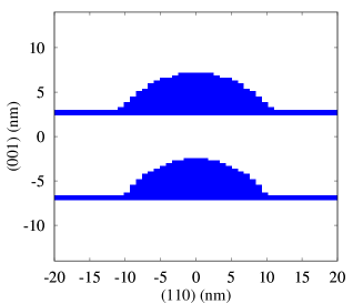
Figure 1: Material distribution in the system.

The system under study is made up of two vertically stacked InGaAs/GaAs self-assembled QDs resting on wetting layers. We assume lens shape of the upper (u) and lower (l) dot. In our calculations we take height $h=4.2$ nm (the same for both dots) and base radii $r_{\mathrm{l}}=10.2$ nm, $r_{\mathrm{u}}=10.8$ nm. The local InAs content in each QD and in the wetting layers is $80$% InAs, the matrix contains $100$% GaAs. The cross section of the InGaAs distribution is shown in Fig. 1.

The Hamiltonian of a system of carriers coupled to LO phonons is

$$H=H_{\mathrm{0}}+V_{\mathrm{c}}+V_{\mathrm{ef}}+H_{\mathrm{ph}}+H_{\mathrm{F}},$$

where $H_{\mathrm{0}}$ describes the single particle states, $V_{\mathrm{c}}$ is the Coulomb interaction between the particles, $V_{\mathrm{ef}}$ represents an axial electric field, $H_{\mathrm{ph}}$ is the Hamiltonian of the LO phonon bath and $H_{\mathrm{F}}$ is a Fröhlich interaction between carriers and LO phonons.

The first term of the Hamiltonian is

$$H_{\mathrm{0}}=\sum_{n}\epsilon^{(\mathit{e})}_{n}a^{\dagger}_{n}a_{n}+\sum_{m}\epsilon^{(\mathit{h})}_{m}h^{\dagger}_{m}h_{m},$$

where $\epsilon^{(\mathit{e})}_{n}$/$\epsilon^{(\mathit{h})}_{m}$ are the energies of the electron/hole states obtained from the $8$ band $\bm{k}\!\cdot\!\bm{p}$ calculations, $a^{\dagger}_{n}$/$h^{\dagger}_{m}$, $a_{n}$/$h_{m}$ are the creation and annihilation operators of the electron/hole in the state $n/m$, respectively. The details of the model are described in Ref. gawarecki14, .

The Coulomb interaction is

$$V_{\mathrm{c}}=\sum_{nn^{\prime}\\ mm^{\prime}}v_{nmm^{\prime}n^{\prime}}a^{\dagger}_{n}h^{\dagger}_{m}h_{m^{\prime}}a_{n^{\prime}},$$

where

$$v_{nmm^{\prime}n^{\prime}}= -\frac{e^{2}}{4\pi\epsilon_{0}\epsilon_{\infty}}\int d{\bm{r}}\int d{\bm{r}}^{\prime}\Psi^{*(\mathit{e})}_{n}({\bm{r}})\Psi^{*(\mathit{h})}_{m}({\bm{r}}^{\prime})$$

$$\times\frac{1}{|{\bm{r}}-{\bm{r}}^{\prime}|}\Psi^{(\mathit{h})}_{m^{\prime}}({\bm{r}}^{\prime})\Psi^{(\mathit{e})}_{n^{\prime}}({\bm{r}}).$$

Here $e$ is the electron charge, $\epsilon_{0}$ and $\epsilon_{\infty}$ are vacuum permittivity and high frequency dielectric constant, $\Psi^{(\mathit{e})}_{n}({\bm{r}})$/$\Psi^{(\mathit{h})}_{m}({\bm{r}}^{\prime})$ corresponds to the electron/hole wave functions which, according to our $\bm{k}\!\cdot\!\bm{p}$ model, are $8$ components spinors. For the sake of efficiency, we calculate $v_{nmm^{\prime}n^{\prime}}$ in the inverse space (see details in Ref. daniels13, ).

The potential of an axial electric field is defined by

$$V_{\mathrm{ef}}=\sum_{nn^{\prime}}Z^{(\mathit{e})}_{nn^{\prime}}a^{\dagger}_{n}a_{n^{\prime}}-\sum_{mm^{\prime}}Z^{(\mathit{h})}_{mm^{\prime}}h^{\dagger}_{m}h_{m^{\prime}},$$

where

$$Z^{(\textit{e}/\textit{h})}_{ij}=F_{z}\int d{\bm{r}}\Psi^{*(\textit{e}/\textit{h})}_{i}({\bm{r}})z\Psi^{(\textit{e}/\textit{h})}_{j}({\bm{r}})$$

and $F_{z}$ is the magnitude of the electric field and $H_{z}$ is the size of our computational domain in the $z$ direction.

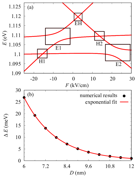
Figure 2: (a) Exciton energy branches as a function of external axial electric field. (b) The width of the anticrossing E2 as a function of the inter-dot distance.

In our calculations, we first find the single-particle states using the $\bm{k}\!\cdot\!\bm{p}$ model. The strain distribution in the system is taken into account within the standard continuous elasticity frameworkpryor98b . Piezoelectricity is included up to the second order in strain tensor elementsbester06 using parameters from Ref. caro15, . In order to find electron and hole states, we perform the calculation using the 8-band $\bm{k}\!\cdot\!\bm{p}$ method in the envelope function approximation. The calculation details have been widely described in Refs. gawarecki14, ; andrzejewski10, and material parameters are taken from Ref. vurgraftman03, . Having the single-particle states we then compute the exciton states which are found using the configuration interaction (CI) method. The axial field is included at the CI stage swiderski16 . Due to numerical efficiency reasons we limit our basis to $4$ lowest electron and hole states (i.e. electron and hole $s$-shell in the lower and in the upper dot). The exciton spectrum obtained in this way is presented in Fig. 2(a). This well-known spectrum of excitons in an electric field szafran05 ; szafran08 is composed of spatially direct and indirect exciton states, clearly distinguishable by the small and large slope of the field dependence of their energies, respectively. If two such states are tuned into the resonance (and if the symmetry of the states is such that selection rules are met) avoided crossing appears in the energy spectrumszafran05 ; szafran08 ; bracker05 ; krenner05b ; muller12 . In Fig. 2(a) these resonance structures are marked by E1,E2 (electron tunneling resonance), H1,H2 (hole tunneling) and EH (very weak coupling between two indirect configurations). We note that extending the basis would lead to a more complex pattern including Coulomb resonances daniels13 ; ardelt16 . Fig. 2(b) shows the electron avoided crossing width (E2) as a function of the distance $D$ between the dots. The dependence follows the exponential lawbayer02b . We obtained an excellent fit for $f(D)=a\exp(-bD)$ with $a=0.751$ eV and $b=0.555$ eV/nm.

II.2 LO phonons

In the polaron formation we assume non-dispersive LO phonon modes with $\hbar\Omega=36$ meV. The LO phonon bath is then described by the Hamiltonian

$$H_{\mathrm{ph}}=\sum_{\bm{q}}\hbar\Omega b^{\dagger}_{\bm{q}}b_{\bm{q}},$$

where $b^{\dagger}_{\bm{q}}$ and $b_{\bm{q}}$ are, respectively, the creation and annihilation operators for the LO phonon mode $\bm{q}$. The carrier-phonon coupling is modeled by the Fröhlich Hamiltonian,

$$H_{\mathrm{F}}= -\sum_{\bm{q}}\frac{e}{q}\sqrt{\frac{\hbar\Omega}{2V\widetilde{\epsilon}\epsilon_{0}}}\left(\sum_{nn^{\prime}}\mathcal{F}^{(\mathit{e})}_{nn^{\prime}}(\bm{q})a^{\dagger}_{n}a_{n^{\prime}}\right.$$

$$\left.-\sum_{mm^{\prime}}\mathcal{F}^{(\mathit{h})}_{mm^{\prime}}(\bm{q})h^{\dagger}_{m}h_{m^{\prime}}\right)\left(b^{\phantom{\dagger}}_{\bm{q}}+b^{\dagger}_{\bm{-q}}\right),$$

where $\widetilde{\epsilon}=(1/\epsilon_{\infty}-1/\epsilon_{s})^{-1}$, $\epsilon_{s}$ is a static dielectric constant in GaAs, $V$ is the normalization volume for phonon modes and $\mathcal{F}^{(\textit{e}/\textit{h})}_{nn^{\prime}}(\bm{q})=\mathcal{F}^{(\textit{e}/\textit{h})*}_{n^{\prime}n}(-\bm{q})$ is the one-particle (electron or hole) form-factor,

$$\mathcal{F}^{(\textit{e}/\textit{h})}_{ij}(\bm{q})=\int\Psi^{*(\textit{e}/\textit{h})}_{i}({\bm{r}})\Psi^{(\textit{e}/\textit{h})}_{j}({\bm{r}})e^{i\bm{k}\cdot{\bm{r}}}d{\bm{r}}.$$

We perform calculations for excitonic polaron states in the basis of noninteracting electron and hole configurations $|\nu\rangle=|n\rangle_{\mathrm{el}}\otimes|m\rangle_{\mathrm{h}}$. In this pair-state basis the Fröhlich Hamiltonian for two-particle (exciton) states has the form

$$H_{\mathrm{F}}=-\sum_{\bm{q}}\frac{e}{q}\sqrt{\frac{\hbar\Omega}{2V\widetilde{\epsilon}\epsilon_{0}}}\sum_{\nu\nu^{\prime}}\mathcal{F}^{(\mathit{X})}_{\nu\nu^{\prime}}(\bm{q})|\nu\rangle\!\langle\nu^{\prime}|\left(b^{\phantom{\dagger}}_{\bm{q}}+b^{\dagger}_{\bm{-q}}\right),$$ (1)

where $\mathcal{F}^{(\mathrm{x})}_{\nu\nu^{\prime}}=\mathcal{F}^{(\mathit{e})}_{nn^{\prime}}(\bm{q})\delta_{mm^{\prime}}-\mathcal{F}^{(\mathit{h})}_{mm^{\prime}}(\bm{q})\delta_{nn^{\prime}}$ with $\nu\sim(nm)$, $\nu^{\prime}\sim(n^{\prime}m^{\prime})$.

II.3 Collective modes

The direct diagonalization of the Hamiltonian would imply sampling the $\bm{q}$ space, which is not feasible due to the large number of required $\bm{q}$ points. However, for non-dispersive LO phonon modes, one can use the collective modes method stauber00 . Thus, one defines the collective modes corresponding to the annihilation operators

$$\widetilde{B}_{\nu\mu}=\sum_{\bm{q}}\sqrt{\frac{l_{0}}{V}}\frac{1}{q}\mathcal{F}^{(\mathrm{x})}_{\nu\mu}b^{\phantom{\dagger}}_{\bm{q}},$$

where $l_{0}$ is an arbitrary characteristic length. The Fröhlich Hamiltonian then becomes

$$H_{\mathrm{F}}=\sum_{\nu\mu}\sqrt{\frac{\hbar\Omega e^{2}}{2l_{0}\widetilde{\epsilon}\epsilon_{0}}}|\nu\rangle\!\langle\mu|\widetilde{B}_{\nu\mu}+\mathrm{h.c.}$$ (2)

However, the collective phonon modes $\widetilde{B}_{\nu\mu}$ are not orthonormal in the sense of canonical commutation relations. Indeed, their commutator is

$$A_{(\nu^{\prime}\mu^{\prime})(\nu\mu)}=[\widetilde{B}_{\nu\mu},\widetilde{B}^{\dagger}_{\nu^{\prime}\mu^{\prime}}]=\frac{l_{0}}{V}\sum_{\bm{q}}\frac{1}{q^{2}}\mathcal{F}^{*}_{\nu^{\prime}\mu^{\prime}}(\bm{q})\mathcal{F}_{\nu\mu}(\bm{q})$$ (3)

and is related to the orthogonality of the form-factors, which does not hold in general.

At this point one has to choose between the original approach involving orthogonalization of the modes stauber00 and the alternative method of non-orthogonal modes obreschkow07 . The latter saves one computational step required for orthogonalization but becomes inconvenient when the form-factors defining the modes are not guaranteed to be linearly independent, which is the case, e.g., for the Fock-Darwin model kaczmarkiewicz10 . Here we propose an efficient method of selecting a spanning set of orthogonal modes based on the Gram matrix of form-factors with respect to the appropriate scalar product defined in Eq. (3). The formal details are given in the Appendix.

Thus, as explained in the Appendix, one can construct the set of orthogonal modes $B_{\alpha}$ from the normalized eigenvectors $\bm{u}^{(\alpha)}=(u_{1}^{(\alpha)},u_{2}^{(\alpha)}\ldots)$ of the Gram matrix $A$ [Eq. (3)]. Denoting the corresponding eigenvalues by $\lambda_{\alpha}$ we arrive at the Hamiltonian in the form

$$H_{\mathrm{F}}=\sqrt{\frac{\hbar\Omega e^{2}}{2l_{0}\widetilde{\epsilon}\epsilon_{0}}}\sum_{\alpha\nu\mu}\sqrt{\lambda_{\alpha}}\left(u^{(\alpha)^{*}}_{\nu\mu}B_{\alpha}c^{\dagger}_{\nu}c^{\phantom{\dagger}}_{\mu}+\mathrm{h.c.}\right).$$ (4)

Finally, we diagonalize this Hamiltonian in the space of zero-, one- and two-phonon states

$$|\Psi_{i}\rangle=\sum_{\nu}d_{\nu}|\nu\rangle+\sum_{\nu\alpha}d_{\nu\alpha}B^{\dagger}_{\alpha}|\nu\rangle+\sum_{\nu\alpha\beta}d_{\nu\alpha\beta}\eta_{\alpha\beta}B^{\dagger}_{\alpha}B^{\dagger}_{\beta}|\nu\rangle.$$

Here $\eta_{\alpha\beta}=1/\sqrt{2}$ for $\alpha=\beta$ and $1$ otherwise, and $\nu$ corresponds to the noninteracting electron-hole pair states defined in Sec. II.2. As a result of this procedure, for the exciton-polaron problem with the restricted s-shell basis (as in Fig. 2) the Hamiltonian involves only several orthogonal modes out of the initial $n^{2}$ modes, where $n$ denotes number of exciton states.

III Results

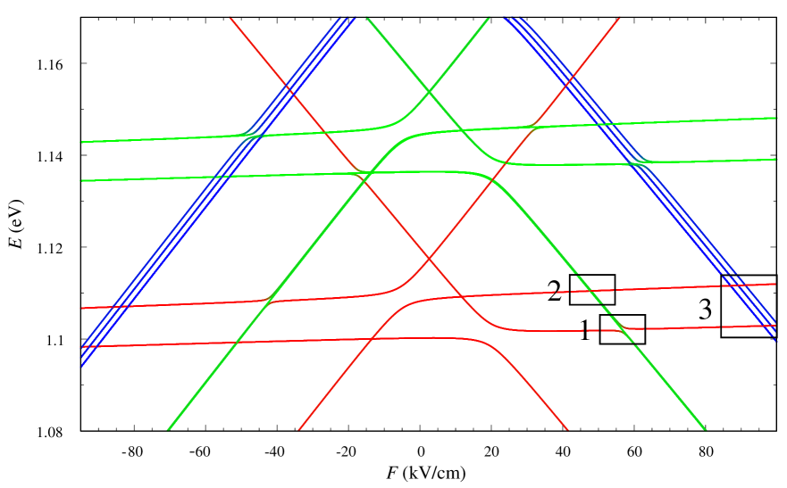
Figure 3: Polaron energy branches as a function of axial electric field at $D=9.6$ nm.

The polaron energy branches were calculated as a function of an axial electric field (Fig. 3). As described in Sec. II, every polaron state $|\Psi_{i}\rangle$ is expressed in the basis of zero-, one- and two-phonon states. We calculated the amplitudes of these components and marked the dominating one in Fig. 3 by assigning colors to the lines: red, green and blue, respectively. The colors are mixed at the resonances involving states with different numbers of phonons. The central part of the plot corresponds to the states with a dominant zero-phonon (pure excitonic) component. They show the same level structure as in Fig. 2 with only a small shift. The same pattern is reflected in $n$-phonon replicas at the energies shifted by approximately $n\hbar\Omega$. Box $1$ contains an avoided level crossing between the direct exciton state (localized in the upper dot) and the single-phonon replica of the indirect exciton state (the hole in the upper dot and the electron in the lower dot). Thus, this anti-crossing corresponds to the resonant electron tunneling combined with emission/absorption of a single LO phonon (decoupled phonon modes do not lead to an anti-crossing). A similar situation takes place for the hole (box $2$). However, for the considered DQD, its coupling strength is much weaker than in the electron case. Furthermore, in contrast to the electron case (which already converges in a small basis), the accurate treatment of the hole-phonon resonances would require larger basis which rapidly increases the computation cost. Therefore, we limit our present discussion to the most pronounced electron-phonon resonances. The resonances marked by the box $3$ involve the coupling to two-phonon states. They occur at very large electric fields and represent a second order processes with much weaker coupling strength compared to the single-phonon case. Furthermore, a proper treatment of two-phonon states requires taking into account $3$-phonon stateskaczmarkiewicz10 . However, neglecting two-phonon states would result in the appearance of non-physical resonances in the single-phonon spectra.

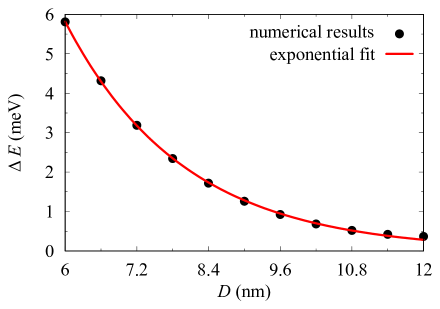
Figure 4: The width of avoided crossing related to electron tunneling combined with emission/absorption of LO phonon (box 1 in Fig. 3).

An interesting question is the dependence of the tunnel coupling strength (extracted from the numerical results as the half-width of the resonant splitting) on the inter-dot distance. The well-known one-dimensional model of tunneling yields exponential dependence. Such a behavior is indeed obtained for an electron in a DQD structure gawarecki10 (which is not obvious, as demonstrated by the hole-related counter-example jaskolski04 ; jaskolski06 ). Therefore, we have investigated the width of the electron-phonon resonance (corresponding to the box $1$) as a function of the distance between the dots. Similarly to the direct tunnel resonance, we obtained an exponential decay (Fig. 4) of the avoided crossing width. The exponential fitting by the function $f(D)=a\exp(-bD)$ yields $a=0.119$ eV and b = $0.503$ eV/nm. Apart from the much lower amplitude, which is expected for a phonon-assisted process, the decay rate $b$ of the polaron resonance is about $10$% lower in comparison to the direct resonance. This could be due to the higher energy of the involved states, and, in consequence, to the deeper penetration into the barrier.

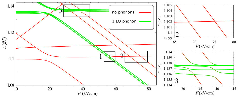
Figure 5: Polaron energy branches as a function of axial electric field at $D=9.6$ nm. The panels on the right show magnified pictures of the corresponding regions.

In the next step, we study the coupling between the electron $p$-shell states located in the upper dot and the phonon replica of the $s$-state from the lower one. To this end, we extended the electron basis to $12$ states ($s$, $p$ shells in each dot) while the hole basis still contains $4$ states. The results are shown in Fig. 5. The basis extension increases the number of orthogonal phonon modes. The exciton-phonon anti-crossing which involves $s$-states (marked in box $1$) has a very similar width (the difference less than $1$%) to that obtained in the reduced basis (box 1 in Fig. 3). The box $2$ contains avoided crossing related to the resonant transition between $s$ and $p$ states of the different dots. Since the angular momentum has to be conserved, this coupling is possible only if the axial symmetry of the system is broken. This can be caused e.g. by the relative displacement of the dotsgawarecki14 , bulk inversion asymmetry (BIA)winkler03 or emerge from the atomistic structurebester05 ; zielinski15 . However, in the present model we assume perfectly aligned dots and the only coupling mechanism is due to BIA and the interface. This leads to narrow avoided crossings visible in box $2$. On the other hand, phonons carry angular momentum and can couple states with different values of the angular momentum. In consequence, we observe the pronounced anti-crossings between the electron states from $p$-shell and the phonon replicas of the $s$-shell states (see box $3$). This LO-phonon assisted coupling is much stronger than those resulting from BIA (box $2$).

IV Summary

We calculated polaron states for excitons in self-assembled double quantum dots using realistic wave functions obtained from $\bm{k}\!\cdot\!\bm{p}$ and configuration-interaction calculations. We proposed a mode orthogonalization scheme that yields a spanning set of effectively coupled collective modes. We investigated resonances (avoided level crossings) related to the electron resonant tunneling combined with emission/absorption of an LO phonon. We have found that the strength of this LO-phonon mediated coupling shows exponential dependence on the inter-dot distance, like in the one-dimensional tunneling problem, with a characteristic length comparable to the direct (zero-phonon) tunneling resonance but with a smaller amplitude. We have also shown that LO phonon modes can efficiently couple states that belong to different shells ($s$ and $p$) from different dots. In this case, direct resonance is strongly suppressed by angular momentum selection rules, while the LO-phonon-assisted coupling is allowed and has a larger amplitude.

Appendix A Orthogonal phonon modes

In this appendix we present a computationally effective procedure of identifying a set of orthogonal collective modes that span the space of all the phonon modes coupled to the carrier subsystem. We will use the combined index $i=(\mu,\nu)$ for the form-factors and define the scalar product

$$\left(\mathcal{F}_{i},\mathcal{F}_{i^{\prime}}\right)=\sum_{\bm{q}}\frac{l_{0}}{Vq^{2}}\mathcal{F}_{i}^{*}(\bm{q})\mathcal{F}_{i^{\prime}}(\bm{q}).$$

In the sense of this scalar product, the matrix $A$ defined in Sec. II.3 is the Gram matrix of the functions $\mathcal{F}_{i}$, $A_{ij}=(\mathcal{F}_{i},\mathcal{F}_{j})$. Being a Gram matrix, it is obviously hermitian and also positive semi-definite: for any vector $\bm{u}=(u_{1},u_{2},\ldots)$,

$$\bm{u}^{{\dagger}}A\bm{u}=\left(\sum_{i}u_{i}\mathcal{F}_{i},\sum_{i}u_{i}\mathcal{F}_{i}\right)\geq 0.$$ (5)

It is known that the Gram matrix carries information on the linear dependence of the system of vectors. Specifically, the set of form factors $\mathcal{F}_{i}$ satisfies a linear dependence relation $\sum_{i}u_{i}\mathcal{F}_{i}=0$ if and only if $\bm{u}=(u_{1},u_{2},\ldots)$ is in the kernel of $A$. Indeed, from Eq. (5), such linear dependence implies $\bm{u}^{{\dagger}}A\bm{u}=0$. For a positive semi-definite matrix this is only possible if $\bm{u}$ is in the kernel. Conversely $A\bm{u}=0$ implies $\sum_{i}(\mathcal{F}_{j},\mathcal{F}_{i})u_{i}=0$, hence $(\sum_{j}u_{j}\mathcal{F}_{j},\sum_{i}u_{i}\mathcal{F}_{i})=0$, which means that $\sum_{i}u_{i}\mathcal{F}_{i}=0$.

This algebraic structure allows us to express the Fröhlich Hamiltonian in terms of a set of orthogonal modes at a cost of generating and diagonalizing the Gram matrix $A$, the size of which is typically rather modest. Assume that $\bm{u}^{(\alpha)}$ are normalized eigenvectors of $A$ with eigenvalues $\lambda_{\alpha}$, that is, $A\bm{u}^{(\alpha)}=\lambda_{a}\bm{u}^{(\alpha)}$. Define $\tilde{\mathcal{G}}_{\alpha}=\sum_{i}u_{i}^{(\alpha)}\mathcal{F}_{i}$. Clearly, from the statement demonstrated above, $\tilde{\mathcal{G}}_{\alpha}=0$ if and only if $\lambda_{\alpha}=0$. One easily shows that $(\tilde{\mathcal{G}}_{\alpha},\tilde{\mathcal{G}}_{\alpha^{\prime}})=\lambda_{\alpha}\delta_{\alpha\alpha^{\prime}}$. For $\alpha$ such that $\lambda_{\alpha}\neq 0$, define the normalized mode function $\mathcal{G}_{\alpha}=\tilde{\mathcal{G}}_{\alpha}/\sqrt{\lambda_{\alpha}}$ and the modes

$$B_{\alpha}=\sum_{\bm{q}}\sqrt{\frac{l_{0}}{V}}\frac{1}{q}\mathcal{G}_{\alpha}(\bm{q})b_{\bm{q}}.$$ (6)

These modes are orthogonal, i.e., they satisfy the canonical commutation relations $[B_{\alpha},B_{\alpha^{\prime}}^{{\dagger}}]=\delta_{\alpha\alpha^{\prime}}$ etc. On the other hand, completeness of the set $\{\bm{u}^{(\alpha)}\}$ implies that $\mathcal{F}_{i}=\sum_{\alpha}u_{i}^{(\alpha)}\tilde{\mathcal{G}}_{\alpha}$. Substituting this to the Fröhlich Hamiltonian [Eq. (1)] (the treatment of the single-particle Hamiltonian is the same), one arrives at the final form of the Fröhlich Hamiltonian expressed in terms of the orthogonal modes, given in Eq. (4).

References

- (1) N. Zhuo, F. Q. Liu, J. C. Zhang, L. J. Wang, J. Q. Liu, S. Q. Zhai, and Z. G. Wang, Nanoscale Res. Lett. 9, 144 (2014).
- (2) R. D. Schaller and V. I. Klimov, Phys. Rev. Lett. 92, 186601 (2004).
- (3) S. Hameau, Y. Guldner, O. Verzelen, R. Ferreira, G. Bastard, J. Zeman, A. Lemaître, and J. M. Gérard, Phys. Rev. Lett. 83, 4152 (1999).
- (4) S. Hameau, J. N. Isaia, Y. Guldner, E. Deleporte, O. Verzelen, R. Ferreira, G. Bastard, J. Zeman, and J. M. Gérard, Phys. Rev. B 65, 085316 (2002).
- (5) P. Kaczmarkiewicz and P. Machnikowski, Phys. Rev. B 81, 115317 (2010).
- (6) T. Stauber, R. Zimmermann, and H. Castella, Phys. Rev. B 62, 7336 (2000).
- (7) O. Verzelen, R. Ferreira, and G. Bastard, Phys. Rev. Lett. 88, 146803 (2002).
- (8) O. Verzelen, R. Ferreira, and G. Bastard, Phys. Rev. B 62, R4809 (2000).
- (9) L. Jacak, J. Krasnyj, D. Jacak, and P. Machnikowski, Phys. Rev. B 65, 113305 (2002).
- (10) O. Verzelen, G. Bastard, and R. Ferreira, Phys. Rev. B 66, 081308(R) (2002).
- (11) E. A. Zibik, L. R. Wilson, R. P. Green, G. Bastard, R. Ferreira, P. J. Phillips, D. A. Carder, J.-P. R. Wells, J. W. Cockburn, M. S. Skolnick, M. J. Steer, and M. Hopkinson, Phys. Rev. B 70, 161305(R) (2004).
- (12) E. A. Zibik, T. Grange, B. A. Carpenter, N. E. Porter, R. Ferreira, G. Bastard, D. S. S. Winnerl, M. Helm, H. Y. Liu, M. S. Skolnick, and L. R. Wilson, Nature Materials 8, 803 (2009).
- (13) B. Szafran, T. Chwiej, F. M. Peeters, S. Bednarek, J. Adamowski, and B. Partoens, Phys. Rev. B 71, 205316 (2005).
- (14) B. Szafran, Acta Phys. Polon. A 114, 1013 (2008).
- (15) H. J. Krenner, M. Sabathil, E. C. Clark, A. Kress, D. Schuh, M. Bichler, G. Abstreiter, and J. J. Finley, Phys. Rev. Lett. 94, 057402 (2005).
- (16) A. S. Bracker, M. Scheibner, M. F. Doty, E. A. Stinaff, I. V. Ponomarev, J. C. Kim, L. J. Whitman, T. L. Reinecke, and D. Gammon, Applied Physics Letters 89, 233110 (2006).
- (17) K. Müller, A. Bechtold, C. Ruppert, M. Zecherle, G. Reithmaier, M. Bichler, H. J. Krenner, G. Abstreiter, A. W. Holleitner, J. M. Villas-Boas, M. Betz, and J. J. Finley, Phys. Rev. Lett. 108, 197402 (2012).
- (18) P.-L. Ardelt, K. Gawarecki, K. Müller, A. M. Waeber, A. Bechtold, K. Oberhofer, J. M. Daniels, F. Klotz, M. Bichler, T. Kuhn, H. J. Krenner, P. Machnikowski, and J. J. Finley, Phys. Rev. Lett. 116, 077401 (2016).
- (19) C. Pryor, J. Kim, L. W. Wang, A. J. Williamson, and A. Zunger, J. Appl. Phys. 83, 2548 (1998).
- (20) K. Gawarecki, P. Machnikowski, and T. Kuhn, Physical Review B 90, 085437 (2014).
- (21) J. M. Daniels, P. Machnikowski, and T. Kuhn, Phys. Rev. B 88, 205307 (2013).
- (22) G. Bester, A. Zunger, X. Wu, and D. Vanderbilt, Phys. Rev. B 74, 081305 (2006).
- (23) M. A. Caro, S. Schulz, and E. P. O‘Reilly, Phys. Rev. B 91, 075203 (2015).
- (24) J. Andrzejewski, G. Sek, E. O‘Reilly, A. Fiore, and J. Misiewicz, J. Appl. Phys. 107, 073509 (2010).
- (25) I. Vurgaftman and J. R. Meyer, Journal of Applied Physics 94, 3675 (2003).
- (26) M. Świderski and M. Zieliński, Acta Phys. Polon. A 129, 7982 (2016).
- (27) Since the LO-phonon coupling is not included explicitly in this calculation, we have replaced by in to account for the LO-phonon induced contribution to the screening.
- (28) M. Bayer, G. Ortner, O. Stern, A. Kuther, A. A. Gorbunov, A. Forchel, P. Hawrylak, S. Fafard, K. Hinzer, T. L. Reinecke, S. N. Walck, J. P. Reithmaier, F. Klopf, and F. Schäfer, Phys. Rev. B 65, 195315 (2002).
- (29) D. Obreschkow, F. Michelini, S. Dalessi, E. Kapon, and M.-A. Dupertuis, Phys. Rev. B 76, 035329 (2007).
- (30) K. Gawarecki, M. Pochwała, A. Grodecka-Grad, and P. Machnikowski, Phys. Rev. B 81, 245312 (2010).
- (31) W. Jaskólski and M. Zieliński, Acta Phys. Polon. A 106, 193 (2004).
- (32) W. Jaskolski, M. Zielinski, G. W. Bryant, and J. Aizpurua, Phys. Rev. B 74, 195339 (2006).
- (33) R. Winkler, Spin-Orbit Coupling Effects in Two-Dimensional Electron and Hole Systems, Vol. 191 of Springer Tracts in Modern Physics (Springer, Berlin, 2003).
- (34) G. Bester and A. Zunger, Phys. Rev. B 71, 045318 (2005).
- (35) M. Zieliński, Y. Don, and D. Gershoni, Phys. Rev. B 91, 085403 (2015).