Evaluating QBF Solvers:
Quantifier Alternations Matter

Abstract

We present an experimental study of the effects of quantifier alternations on the evaluation of quantified Boolean formula (QBF) solvers. The number of quantifier alternations in a QBF in prenex conjunctive normal form (PCNF) is directly related to the theoretical hardness of the respective QBF satisfiability problem in the polynomial hierarchy. We show empirically that the performance of solvers based on different solving paradigms substantially varies depending on the numbers of alternations in PCNFs. In related theoretical work, quantifier alternations have become the focus of understanding the strengths and weaknesses of various QBF proof systems implemented in solvers. Our results motivate the development of methods to evaluate orthogonal solving paradigms by taking quantifier alternations into account. This is necessary to showcase the broad range of existing QBF solving paradigms for practical QBF applications. Moreover, we highlight the potential of combining different approaches and QBF proof systems in solvers.

1 Introduction

The logic of quantified Boolean formulas (QBFs) [33] extends propositional logic by existential and universal quantification of propositional variables. Consequently, the QBF satisfiability problem is PSPACE-complete [48]. QBF satisfiability is a restricted form of a quantified constraint satisfaction problem (QCSP), cf. [13, 16, 17, 40], where all variables are defined over a Boolean domain.

The polynomial hierarchy (PH) [41, 47, 52] allows to describe the complexity of problems that are beyond the classes P and NP. The satisfiability problem of a QBF $\psi$ in prenex conjunctive normal form (PCNF) with $k\geq 0$ quantifier alternations is located at level $k+1$ of PH [47, 52] and either $\Sigma_{k+1}^{P}$-complete or $\Pi_{k+1}^{P}$-complete, depending on the first quantifier in $\psi$. Due to this property, practically relevant problems from any level of PH up to the class PSPACE (here with arbitrarily nested quantifiers) can succinctly be encoded as QBFs.

Efficient solvers are highly requested to solve QBF encodings of problems. Competitions like QBFEVAL or the QBF Galleries have been driving solver development [23, 29, 38]. State-of-the-art solvers are based on solving paradigms like, e.g., expansion [2, 10, 30] or Q-resolution [34]. These two paradigms are orthogonal by proof complexity [7, 31, 49]. Informally, orthogonal paradigms have complementary strengths on certain families of formulas.

Motivated by the variety of available QBF solving paradigms and solvers, we present an experimental study of the effects of quantifier alternations on the evaluation of QBF solvers. To this end, we consider benchmarks, solvers, and preprocessors from QBFEVAL’17 [43]. As our main result, we show that the performance of solvers based on different and, notably, orthogonal solving paradigms substantially varies depending on the numbers of alternations. Instances with a particular number of alternations may be overrepresented (i.e., appear more frequently) in a benchmark set, thus resulting in alternation bias. In this case, overall solver rankings by total solved instances may not provide a comprehensive picture as they might only reflect the strengths of certain solvers on overrepresented instances, but not the (perhaps orthogonal) strengths of other solvers on underrepresented ones.

In related work [39], the correlation between solver performance and various syntactic features such as treewidth [1, 44] was analyzed. In contrast to that, we do not study such correlations. By our study we a posteriori highlight diversity of solver performance based on the single feature of alternations, which are naturally related to the theoretical hardness of instances in PH. Recently, alternations have become of interest also in theoretical work on QBF proof complexity [6, 9, 18].

We aim at raising the awareness and importance of quantifier alternations in comparative studies of QBF solver performance and the potential negative impact on the progress of QBF solver development. If solvers are evaluated on benchmark sets with alternation bias and alternations are neglected in the analysis, then future research may inadvertently be narrowed down to only exploring approaches that perform well on overrepresented instances with a certain number of alternations. The risk of such detrimental effects on a research field driven by empirical analysis has been pointed already in the early days of propositional satisfiability (SAT) solving [27] and also with respect to more recent SAT solver competitions [3, 4, 5]. In contrast to the NP-completeness of SAT, the complexity landscape of QBF encodings defined by PH is more diverse, which gives rise to several sources of inadvertent convergence of research lines.

In addition to focusing on alternations, we report on virtual best solver (VBS) statistics, where the VBS solved between 50% and 70% more instances than the single overall best solver on a benchmark set. These results indicate the potential of combining orthogonal QBF proof systems in solvers. Moreover, we point out that overall low-ranked solvers potentially solve more instances uniquely and have larger contributions to the VBS than high-ranked ones. Similar observations were made in the context of SAT solver competitions [53].

The majority of benchmarks in QBFLIB [23], the QBF research community portal, has no more than two quantifier alternations. Hence problems from the first three levels in PH have been, and are, of primary interest to practitioners. However, to strengthen QBF solving as a key technology for solving problems from any levels of PH up to PSPACE-complete problems, QBF solvers must be improved on instances with any number of alternations. Our empirical study motivates the development of methods to evaluate orthogonal solving paradigms by taking quantifier alternations into account. This is necessary to showcase the broad range of existing paradigms for practical QBF applications.

2 Preliminaries

We consider QBFs $\psi:=\Pi.\phi$ in prenex conjunctive normal form (PCNF) consisting of a quantifier prefix $\Pi:=Q_{1}B_{1}\ldots Q_{n}B_{n}$ and a quantifier-free propositional formula $\phi$ in CNF. A CNF consists of a conjunction of clauses. A clause is a disjunction of literals. A literal is either a propositional variable $x$ or its negation $\neg x$. The prefix $\Pi$ is a linearly ordered sequence of quantifier blocks (qblocks) $Q_{i}B_{i}$, where $Q_{i}\in\{\forall,\exists\}$ is a quantifier and $B_{i}$ is a block (i.e., a set) of propositional variables with $B_{i}\cap B_{j}=\emptyset$ for $i\not=j$. The notation $Q_{i}B_{i}$ is shorthand for $Q_{i}x_{1}\ldots Q_{i}x_{m}$ for all $x_{j}\in B_{i}$. Formula $\phi$ is defined precisely over the variables that appear in $\Pi$. If $Q_{i}=Q_{i+1}$ then $B_{i}$ and $B_{i+1}$ are merged to obtain $Q_{i}(B_{i}\cup B_{i+1})$. Hence adjacent qblocks are quantified differently. Without loss of generality, we assume that the innermost quantifier $Q_{n}=\exists$ is existential. (If $Q_{n}=\forall$ then $B_{n}$ is eliminated by universal reduction [34].) A PCNF with $n$ qblocks has $n-1$ quantifier alternations.

The semantics of PCNFs are defined recursively. The PCNF consisting only of the syntactic truth constant $\top$ ($\bot$) is satisfiable (unsatisfiable). A PCNF $\psi:=Q_{1}B_{1}\ldots Q_{n}B_{n}.\phi$ with $Q_{1}=\exists$ ($Q_{1}=\forall$) is satisfiable iff, for $x\in B_{1}$, $\psi[x]$ or (and) $\psi[\neg x]$ is satisfiable, where $\psi[x]$ ($\psi[\neg x]$) is the PCNF obtained from $\psi$ by replacing all occurrences of $x$ by $\top$ ($\bot$) and deleting $x$ from $B_{1}$.

To make the presentation of our experimental study self-contained, we introduce QBF proof systems only informally and refer to a standard, formal definition of propositional proof systems [20]. A QBF proof system $\mathcal{PS}$ is a formal system consisting of inference rules. The inference rules allow to derive new formulas (e.g. clauses) from a given QBF $\psi$ and from previously derived formulas. A QBF proof system $\mathcal{PS}$ is correct if, for any QBF $\psi$, it holds that if the formula $\bot$ (false, e.g., the empty clause) is derivable in $\mathcal{PS}$ from $\psi$ then $\psi$ is unsatisfiable. A QBF proof system $\mathcal{PS}$ is complete if, for any QBF $\psi$, it holds that if $\psi$ is unsatisfiable then $\bot$ is derivable in $\mathcal{PS}$ from $\psi$. A proof $P$ of an unsatisfiable QBF $\psi$ in $\mathcal{PS}$ is a sequence of given formulas and formulas derived by inference rules ending in $\bot$. The length $|P|$ of a proof $P$ is the sum of the sizes of all formulas in $P$.

Let $\mathcal{PS}$ and $\mathcal{PS^{\prime}}$ be QBF proof systems and $\Psi$ be a family of unsatisfiable QBFs. Let $P$ be a proof of some QBF $\psi\in\Psi$ in $\mathcal{PS}$ such that the length $|P|$ of $P$ is polynomial in the size of $\psi$. Assume that the length $|P^{\prime}|$ of every proof $P^{\prime}$ of $\psi\in\Psi$ in $\mathcal{PS^{\prime}}$ is exponential in the size of $\psi$. Then $\mathcal{PS}$ is stronger than $\mathcal{PS}^{\prime}$ with respect to family $\Psi$. Two QBF proof systems $\mathcal{PS}$ and $\mathcal{PS^{\prime}}$ are orthogonal if $\mathcal{PS}$ is stronger than $\mathcal{PS}^{\prime}$ with respect to a family $\Psi$ and $\mathcal{PS}^{\prime}$ is stronger than $\mathcal{PS}$ with respect to some other family $\Psi^{\prime}$. The relation between QBF proof systems in terms of their strengths is studied in the research field of QBF proof complexity.

QBF proof systems are the formal foundation of QBF solver implementations. Expansion [2, 10, 30] and Q-resolution [34] are traditional QBF proof systems that are orthogonal [7, 31, 49]. Orthogonal proof systems are of particular interest for practical QBF solving since they give rise to solvers that have individual, complementary strengths on certain families of formulas. In our experiments, we highlight the potential of combining orthogonal proof systems in QBF solvers.

3 Experimental Setup

For our experimental study we use the set $S_{17\mid 523}$ containing 523 PCNFs from QBFEVAL’17 [43]. Partitioning $S_{17\mid 523}$ by numbers of qblocks results in 64 classes. Table 1 shows a histogram of $S_{17\mid 523}$ by the numbers of formulas (#f) in

#q	#f	$\#\textnormal{f}_{\textnormal{L}}$
1	0	253
2	90	7,319
3	236	4,110
4–10	70	2,185
11–20	42	437
21–	85	2,444
1–3	326	11,682
4–	197	5,066

Table 1:

classes defined by the number of qblocks (#q). Instances with up to three qblocks (row “1–3”) amount to 62% of all instances and hence are overrepresented in $S_{17\mid 523}$. To generate $S_{17\mid 523}$, instances were sampled from instance categories in QBFLIB in addition to newly submitted ones based on empirical hardness results from previous competitions. We also computed a histogram of a QBFLIB snapshot containing 16,748 instances (column $\#\textnormal{f}_{\textnormal{L}}$ in Table 1). Instances with no more than three qblocks (row “1–3”) are also overrepresented (69%) in that snapshot. Hence alternation bias in $S_{17\mid 523}$ follows from a related bias in QBFLIB, which is due to the focus of QBF practitioners on problems located at low levels in PH. Moreover, the bias does not result from a flawed selection of competition instances. We use the terminology “overrepresented” and “bias” for the statistical fact that instances with few qblocks appear more frequently in $S_{17\mid 523}$.

In order to evaluate the impact of qblocks on solver performance, we consider 11 solvers that participated in QBFEVAL’17 and were top-ranked. The solvers implement the following six different solving paradigms:

1. Expansion [2, 10] eliminates variables from a PCNF $\psi$ until the formula reduces to either true or false. RAReQS 1.1 [30] applies recursive expansion based on counterexample-guided abstraction refinement (CEGAR) [19], while Ijtihad operates in a non-recursive way. Rev-Qfun 0.1 [28] extends RAReQS by machine learning techniques, and DynQBF [15] exploits QBF tree decompositions. Theoretical properties of expansion as a proof system, which underlies implementations of expansion solvers, have been intensively studied [7, 31].

2. QDPLL [14] is a backtracking search procedure that generalizes the DPLL algorithm [21]. GhostQ [30, 35] combines QDPLL with clause and cube learning (a cube is a conjunction of literals) based on the Q-resolution proof system [34]. Additionally, it reconstructs the structure of PCNFs encoded by Tseitin translation [50], and applies CEGAR-based learning.

3. Nested SAT solving uses one SAT solver per qblock in a PCNF, where universal quantification is handled as negated existential quantification. The solver QSTS [11, 12] combines nested SAT solving with structure reconstruction. Propositional resolution is the proof system that underlies SAT solving.

4. Clause selection and clausal abstraction as implemented in the solvers QESTO 1.0 [32] and CAQE [45, 49], respectively, decompose the given PCNF into a sequence of propositional formulas and apply CEGAR techniques. The proof system implemented in CAQE has been presented recently [49].

5. Backtracking search with clause and cube learning (QCDCL) [24, 25, 36, 54] based on Q-resolution extends the CDCL approach for SAT solving [46] to QBFs. The solver DepQBF [37] implements QCDCL with generalized Q-resolution axioms allowing for a stronger calculus to derive learned clauses and cubes. Qute [42] learns variable dependencies lazily in a run.

6. Heretic is based on a hybrid approach that combines expansion and QCDCL in a sequential portfolio style. Thereby, the QCDCL solver DepQBF is applied to learn clauses from the given QBF, which are then heuristically added to the expansion solver Ijtihad.

4 Experimental Results

We illustrate a substantial performance diversity of the above solvers from QBFEVAL’17 on instances with different numbers of quantifier alternations. To this end, we rank solvers based on instance classes given by numbers of qblocks similar to Table 1. Our empirical results are consistent on instances with and without preprocessing by the state-of-the-art tools Bloqqer [26] and HQSpre [51]. Alternation bias in original instances is present also in preprocessed ones. Unless stated otherwise, all experiments were run on Intel Xeon CPUs (E5-2650v4, 2.20 GHz) with Ubuntu 16.04.1 using CPU time and memory limits of 1800 seconds and seven GB. Exceeding the memory limit is counted as a time out.

It is well known that preprocessing may have positive effects on the performance of certain solvers while negative effects on others (cf. [38, 39]). To compensate for these effects, we applied preprocessing both to filter the original benchmark set $S_{17\mid 523}$ and to preprocess instances. Many preprocessing techniques used to simplify a QBF by eliminating clauses and literals are restricted variants of solving approaches, hence instances might be solved already by preprocessing.

We ran Bloqqer (version 37) with a time limit of two hours as a filter on set $S_{17\mid 523}$ to obtain the set $S_{17\mid 437}$ containing 437 original PCNFs, where we discarded 76 instances from $S_{17\mid 523}$ that were solved already by Bloqqer and ten instances that became propositional, i.e., which ended up having a single quantifier block of existential variables only. Bloqqer exceeded the time limit on 39 instances, which we included in their original form in set $S_{17\mid 437}$.

In a similar way, we filtered set $S_{17\mid 523}$ using HQSpre to obtain the set $S_{17\mid 312}$ containing 312 original instances, where we discarded 183 instances solved by HQSpre and 28 which became propositional, and we included 42 original ones in $S_{17\mid 312}$ where HQSpre exceeded the resource limits. We did not consider a variant of HQSpre that applies a restricted form of preprocessing to preserve gate structure present in formulas [51]. Compared to the unrestricted variant of HQSpre we used, the restricted one did not improve overall solver performance.

By applying Bloqqer and HQSpre to the filtered sets $S_{17\mid 437}$ and $S_{17\mid 312}$ again, we generated the sets $S_{17\mid 437}^{\prime}$ and $S_{17\mid 312}^{\prime}$, respectively, containing preprocessed instances and those original instances where the preprocessors exceeded the resource limits. We disabled any additional use of Bloqqer or HQSpre as separate preprocessing modules integrated in some solvers. In the following, we focus our analysis on the four sets $S_{17\mid 437}$, $S_{17\mid 437}^{\prime}$, $S_{17\mid 312}$, and $S_{17\mid 312}^{\prime}$.

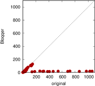
(a) Sets $S_{17\mid 437}$ (x-axis) and $S_{17\mid 437}^{\prime}$.

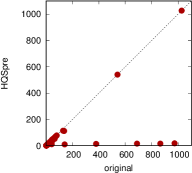
(b) Sets $S_{17\mid 312}$ (x-axis) and $S_{17\mid 312}^{\prime}$.

Figure 1: Numbers of qblocks before (“original”) and after preprocessing by Bloqqer (1a) and HQSpre (1b) on filtered (x-axes) and preprocessed instances (y-axes), respectively.

Table 2: Histograms of the benchmark sets $S_{17\mid 437}$ and $S_{17\mid 437}^{\prime}$ (filtered and preprocessed by Bloqqer), and $S_{17\mid 312}$ and $S_{17\mid 312}^{\prime}$ (filtered and preprocessed by HQSpre) illustrating the numbers of formulas (#f) in classes given by the number of qblocks (#q).

#q	#f
2	63
3	215
4–10	63
11–20	36
21–	60
2–3	278
4–	159

(a) Set $S_{17\mid 437}$.

#q	#f
2	65
3	218
4–10	59
11-20	53
21–	42
2–3	283
4–	154

(b) Set $S_{17\mid 437}^{\prime}$.

#q	#f
2	70
3	145
4–10	26
11–20	30
21–	41
2–3	215
4–	97

(c) Set $S_{17\mid 312}$.

#q	#f
2	70
3	145
4–10	26
11–20	40
21–	31
2–3	215
4–	97

(d) Set $S_{17\mid 312}^{\prime}$.

The application of Bloqqer and HQSpre to sets $S_{17\mid 437}$ and $S_{17\mid 312}$ reduces the number of qblocks in instances considerably. This is illustrated by the scatter plots in Figures 1a and 1b, respectively. The average number of qblocks decreases from 29 in set $S_{17\mid 437}$ to 10 in set $S_{17\mid 437}^{\prime}$. Likewise, the average decreases from 24 in set $S_{17\mid 312}$ to 14 in set $S_{17\mid 312}^{\prime}$. As an extreme case, the number of qblocks in an instance in $S_{17\mid 437}$ was reduced by Bloqqer from 1061 to 19.

In all sets $S_{17\mid 437}$, $S_{17\mid 437}^{\prime}$, $S_{17\mid 312}$, and $S_{17\mid 312}^{\prime}$, the median number of qblocks is three. This is due to alternation bias like in the original set $S_{17\mid 523}$ (Table 1). The related histograms are shown in Tables 1a to 1d, where instances with no more than three qblocks are overrepresented (rows “2–3”) as they amount to between 63% and 68% of all 437, respectively, 312 instances. Set $S_{17\mid 437}$ has 59 classes by numbers of qblocks compared to 45 in set $S_{17\mid 437}^{\prime}$, and set $S_{17\mid 312}$ has 42 compared to 40 in set $S_{17\mid 312}^{\prime}$. Bloqqer reduces the number of instances with 21 or more qblocks (lines “21–”) from 60 in $S_{17\mid 437}$ to 42 in $S_{17\mid 437}^{\prime}$ (Tables 1a and 1b). HQSpre reduces this number from 41 in $S_{17\mid 312}$ to 31 in $S_{17\mid 312}^{\prime}$ (Tables 1c and 1d).

Table 3: Solvers and corresponding paradigms (P) from Section 3, solved instances (S), unsatisfiable ($\bot$) and satisfiable ones ($\top$), total CPU time including time outs, and uniquely solved instances (U) on sets $S_{17\mid 437}$ (2a), $S_{17\mid 437}^{\prime}$ (2b), $S_{17\mid 312}$ (2c), and $S_{17\mid 312}^{\prime}$ (2d).

Solver	P	S	$\bot$	$\top$	Time	U
Rev-Qfun	1	174	106	68	497K	6
GhostQ	2	145	79	66	547K	12
RAReQS	1	126	94	32	577K	4
CAQE	4	126	87	39	578K	6
Heretic	6	122	95	27	580K	0
DepQBF	5	115	78	37	603K	16
Ijtihad	1	110	88	22	599K	1
QSTS	3	103	75	28	618K	3
Qute	5	77	47	30	658K	0
QESTO	4	76	56	20	661K	0
DynQBF	1	47	27	20	714K	9

(a) Set $S_{17\mid 437}$ filtered by Bloqqer.

Solver	P	S	$\bot$	$\top$	Time	U
RAReQS	1	175	127	48	499K	5
CAQE	4	169	114	55	514K	0
Heretic	6	164	119	45	513K	0
Ijtihad	1	136	103	33	555K	2
Rev-Qfun	1	135	92	43	563K	3
QSTS	3	127	98	29	576K	12
QESTO	4	115	84	31	601K	1
DepQBF	5	102	64	38	624K	3
GhostQ	2	82	47	35	661K	1
Qute	5	73	56	17	672K	0
DynQBF	1	65	37	28	684K	25

(b) Set $S_{17\mid 437}^{\prime}$ preprocessed by Bloqqer.

Solver	P	S	$\bot$	$\top$	Time	U
GhostQ	2	112	61	51	373K	15
Rev-Qfun	1	110	58	52	376K	6
CAQE	4	68	42	26	454K	6
DepQBF	5	64	41	23	461K	4
QSTS	3	56	34	22	470K	3
RAReQS	1	50	34	16	482K	1
Heretic	6	49	34	15	485K	0
Qute	5	47	25	22	486K	0
DynQBF	1	46	24	22	488K	9
QESTO	4	45	30	15	491K	0
Ijtihad	1	36	27	9	504K	1

(c) Set $S_{17\mid 312}$ filtered by HQSpre.

Solver	P	S	$\bot$	$\top$	Time	U
CAQE	4	114	65	49	378K	6
RAReQS	1	103	63	40	390K	3
QESTO	4	97	63	34	402K	1
Rev-Qfun	1	90	57	33	414K	6
Heretic	6	87	55	32	424K	0
QSTS	3	72	46	26	448K	1
DepQBF	5	72	44	28	451K	5
Qute	5	70	42	28	449K	2
Ijtihad	1	58	43	15	465K	1
GhostQ	2	58	33	25	475K	0
DynQBF	1	45	24	21	487K	17

(d) Set $S_{17\mid 312}^{\prime}$ preprocessed by HQSpre.

Table 4: Solvers and corresponding solving paradigms (P) as listed in Section 3, solved instances (S, cf. Tables 2a to 2d), average ($\overline{q}$) and median number ($\tilde{q}$) of qblocks of respective solved instances in the considered benchmark sets. Rows “$\bigcup$” show statistics for the total number of instances solved by any solver based on a particular paradigm.

		$S_{17\mid 437}$			$S_{17\mid 437}^{\prime}$			$S_{17\mid 312}$			$S_{17\mid 312}^{\prime}$
P	Solver	S	$\overline{q}$	$\tilde{q}$	S	$\overline{q}$	$\tilde{q}$	S	$\overline{q}$	$\tilde{q}$	S	$\overline{q}$	$\tilde{q}$
1	DynQBF	47	6.1	3.0	65	9.0	3.0	46	4.8	3.0	45	3.3	2.0
	Ijtihad	110	42.1	5.0	136	12.7	3.0	36	40.5	3.0	58	17.6	3.0
	RAReQS	126	39.8	3.0	175	11.2	3.0	50	22.6	3.0	103	11.5	3.0
	Rev-Qfun	174	55.1	3.0	135	12.5	3.0	110	47.4	3.0	90	24.0	3.0
	$\bigcup$	228	45.9	3.0	238	9.6	3.0	145	37.8	3.0	150	16.6	3.0
2	GhostQ	145	12.5	3.0	82	15.8	3.0	112	7.5	3.0	58	8.1	3.0
3	QSTS	103	63.2	5.0	127	15.6	5.0	56	65.3	3.0	72	22.6	3.0
4	CAQE	126	44.3	5.0	169	12.9	3.0	68	37.4	3.0	114	12.0	3.0
	QESTO	76	47.7	3.0	115	15.5	3.0	45	15.6	3.0	97	8.1	3.0
	$\bigcup$	134	41.9	3.5	182	12.5	3.0	74	34.7	3.0	127	11.6	3.0
5	DepQBF	115	45.7	5.0	102	17.8	8.5	64	21.2	8.0	72	10.5	3.0
	Qute	77	30.0	4.0	73	20.7	9.0	47	16.4	3.0	70	9.7	3.0
	$\bigcup$	137	38.8	3.0	117	16.2	6.0	83	17.0	3.0	97	9.2	3.0
6	Heretic	122	39.5	5.0	164	12.5	5.0	49	34.4	3.0	87	14.1	3.0

4.1 Solved Instances: Overall Rankings

We first analyze overall solver performance by ranking solvers according to total numbers of instances solved in the benchmark sets $S_{17\mid 437}$, $S_{17\mid 437}^{\prime}$, $S_{17\mid 312}$, and $S_{17\mid 312}^{\prime}$. Then we show that the strengths of certain solvers and solving paradigms are not reflected in such overall rankings. To highlight these individual strengths, in Section 4.2 below we carry out a more fine-grained analysis of solver performance based on instances that were solved in instance classes defined by their number of qblocks. Our results show that there is a considerable performance diversity between solvers and solving paradigms with respect to classes.

Tables 2a to 2d show overall solver rankings by total numbers of solved instances. Solver performance greatly varies depending on preprocessing. For example, while RAReQS, CAQE, and QESTO clearly benefit from preprocessing, it is harmful for GhostQ and Rev-Qfun. The expansion solvers RAReQS and Rev-Qfun (paradigm 1) dominate the rankings on sets $S_{17\mid 437}$ and $S_{17\mid 437}^{\prime}$ (Tables 2a and 2b), and are ranked second on sets $S_{17\mid 312}$ and $S_{17\mid 312}^{\prime}$ (Tables 2c and 2d). The first three places in the respective rankings of each set are taken by solvers based on paradigms 1, 2, 4, and 6. That is, solvers QSTS, DepQBF, and Qute (paradigms 3 and 5) are not among the three top-performing solvers.

There is a large performance diversity between different solvers based on the same paradigm. For example, the expansion solver DynQBF is ranked last on three sets, which is in contrast to the overall good performance of the expansion solvers RAReQS and Rev-Qfun. Likewise, there is a difference between the QCDCL solvers DepQBF and Qute. Such differences between implementations of the same solving paradigm (or proof system) can be attributed to the fact that the solvers might apply different heuristics to explore the search space to find a proof.

The numbers of instances solved uniquely by a particular solver (columns U in Tables 2a to 2d) highlight the strengths of solvers such as QSTS, DynQBF, and DepQBF which do not show top performance in the overall rankings. Most notably DynQBF by far solved the largest number of instances uniquely on preprocessed sets $S_{17\mid 437}^{\prime}$ (Table 2b) and $S_{17\mid 312}^{\prime}$ (Table 2d). With respect to uniquely solved instances, QSTS is second after DynQBF on set $S_{17\mid 437}^{\prime}$, and DepQBF solved the largest number of instances uniquely on set $S_{17\mid 437}$ (Table 2a).

Towards a more fine-grained analysis of solver performance, we consider the number of qblocks of instances solved by individual solvers and in total by solving paradigms. Table 4 shows related average and median numbers of qblocks. In general, averages are greater for instances from filtered sets ($S_{17\mid 437}$ and $S_{17\mid 312}$) than from preprocessed ones ($S_{17\mid 437}^{\prime}$ and $S_{17\mid 312}^{\prime}$), since preprocessing reduces the numbers of qblocks (cf. Figure 1). The difference in averages between solvers based on the same paradigm, e.g., DynQBF and Rev-Qfun in set $S_{17\mid 437}$, is due to few solved instances having many qblocks (up to more than 1000).

Although the median number of qblocks of instances in every considered set is three (due to alternation bias), the median number of instances solved by certain solvers as shown in Table 4 is greater than three. For example, this is the case for the QCDCL solvers DepQBF and Qute on sets $S_{17\mid 437}$, $S_{17\mid 437}^{\prime}$, and $S_{17\mid 312}$ (DepQBF only). Moreover, QCDCL is the solving paradigm with the greatest median (6.0 in set $S_{17\mid 437}^{\prime}$) among all sets when considering instances solved by any solver based on a particular paradigm (rows “$\bigcup$”). Ijtihad has the greatest median among expansion solvers, QSTS and Heretic have a median of 5.0 on sets $S_{17\mid 437}$ and $S_{17\mid 437}^{\prime}$, and CAQE has a median of 5.0 on set $S_{17\mid 437}$. These statistics indicate that there are solvers which tend to perform well on instances with relatively many qblocks, which however is not reflected in overall rankings in Tables 2a to 2d as many of these solvers are not among the top-performing ones.

Table 5: Instances solved in classes by numbers of qblocks (#q) and numbers of formulas in each class (#f) for sets $S_{17\mid 437}$ (4a), $S_{17\mid 437}^{\prime}$ (4b), $S_{17\mid 312}$ (4c), $S_{17\mid 312}^{\prime}$ (4d). Only class winners (bold face) are shown, paradigms (P:) are indicated in the first row.

P:		1	2	4	6	5
#q	#f	Rev-Qfun	GhostQ	CAQE	Heretic	DepQBF
2	63	17	32	5	2	6
3	215	101	89	56	50	47
4–10	63	25	4	25	34	14
11–20	36	6	3	10	11	20
21–	60	25	17	30	25	28
2–3	278	118	121	61	52	53
4–	159	56	24	65	70	62

(a) Set $S_{17\mid 437}$ filtered by Bloqqer.

P:		1	4	6	1
#q	#f	RAReQS	CAQE	Heretic	DynQBF
2	65	16	15	13	24
3	218	80	81	65	18
4–10	59	37	26	38	13
11-20	53	25	25	31	4
21–	42	17	22	17	6
2–3	283	96	96	78	42
4–	154	79	73	86	23

(b) Set $S_{17\mid 437}^{\prime}$ preprocessed by Bloqqer.

P:		2	1	4	5
#q	#f	GhostQ	Rev-Qfun	CAQE	DepQBF
2	70	36	18	5	7
3	145	62	71	33	23
4–10	26	3	5	7	7
11–20	30	3	5	8	16
21–	41	8	11	15	11
2–3	215	98	89	38	30
4–	97	14	21	30	34

(c) Set $S_{17\mid 312}$ filtered by HQSpre.

P:		4	6	5	1
#q	#f	CAQE	Heretic	DepQBF	DynQBF
2	70	18	15	15	24
3	145	67	42	24	14
4–10	26	6	10	7	5
11–20	40	14	15	20	2
21–	31	9	5	6	0
2–3	215	85	57	39	38
4–	97	29	30	33	7

(d) Set $S_{17\mid 312}^{\prime}$ preprocessed by HQSpre.

4.2 Solved Instances: Class-Based Analysis

Motivated by the above observations related to median numbers of qblocks of solved instances, we aim to provide a more detailed picture of the strengths of the different solvers and implemented solving paradigms. To this end, we analyze the numbers of solved instances in classes defined by their numbers of qblocks.

Tables 4a to 4d show the numbers of instances that were solved in the individual classes in the considered sets. Only class winners are shown (bold face), i.e., solvers that solved the largest number of instances in at least one class, where ties are not broken. The bottom rows of the tables show statistics for instances with up to three (row “2–3”) and more than three qblocks (row “4–”).

The five different class winners Rev-Qfun, GhostQ, CAQE, Heretic, and DepQBF in set $S_{17\mid 437}$ (Table 4a) implement five different solving paradigms (rows P:). In set $S_{17\mid 437}^{\prime}$ (Table 4b) the four class winners implement three different paradigms. In sets $S_{17\mid 312}$ and $S_{17\mid 312}^{\prime}$ (Tables 4c and 4d), there are four different paradigms implemented in the respective four class winners. Overall, with respect to all four benchmark sets, there are seven different solvers out of the 11 considered ones that win in a class. These class winners implement five out of the six paradigms listed in Section 3, all except paradigm 3 implemented in QSTS.

Notably, class winners are not always overall top-ranked, and an overall top-ranked solver does not always win a class. For example, RAReQS is ranked third in set $S_{17\mid 437}$ (Table 2a) and second in set $S_{17\mid 312}^{\prime}$ (Table 2d) but does not win a class in the respective set (Tables 4a and 4d). As an extreme case, DynQBF is ranked last on sets $S_{17\mid 437}^{\prime}$ and $S_{17\mid 312}^{\prime}$ (Tables 2b and 2d) but wins the class of instances with no more than two qblocks (row “2” in Tables 4b and 4d).

Instances with few qblocks are overrepresented in the benchmark sets. Alternation bias of this kind in general bears the risk of masking the strengths of certain solvers on underrepresented instances. The variety of class winners and paradigms shown in Tables 4a to 4d is not reflected when only considering overall solver rankings by total numbers of solved instances in Tables 2a to 2d.

The expansion solvers Rev-Qfun and RAReQS (paradigm 1) tend to perform better on instances with relatively few qblocks, while solvers applying QCDCL (paradigms 5 and 6) tend to perform better on many qblocks. For example, either DepQBF or Heretic win on instances with four or more qblocks (row “4–”) in any set. These statistics are interesting in the context of QBF proof complexity as the proof systems underlying expansion and QCDCL are orthogonal [7, 31]. CAQE based on paradigm 4 wins on instances with 21 or more qblocks (rows “21–”) in all sets (Tables 4a to 4d). Further, it also wins on instances with no more than three qblocks in set $S_{17\mid 312}^{\prime}$ (Table 4d). The proof systems underlying paradigms 4 and 1 (expansion) are orthogonal [49]. The performance diversity of orthogonal proof systems on instances with different numbers of qblocks is not reflected in overall rankings and motivates further, theoretical study in QBF proof complexity.

Due to alternation bias, classes of instances with few qblocks are larger than those with many qblocks. Hence solvers often win in a class of instances with many qblocks by only a small margin. For example, the top-ranked solvers on classes “4–10”, “11–20”, and “21–” tend to be close to each other in terms of solved instances (cf. appendix). Moreover, solvers implementing the same paradigm might show diverse performance due to different heuristics in proof search. To consider these factors, we carry out a class-based analysis of solving paradigms. To this end, we count instances solved by any solver implementing a particular paradigm. This study is related to statistics in rows “$\bigcup$” of Table  4.

Tables 5a to 5d show instances solved by each of the solving paradigms 1 to 6 (first row) in classes of instances. Class winners are highlighted in bold face. Paradigm 1 (expansion) dominates the other paradigms on complete benchmark sets (row “2–”). On instances obtained by Bloqqer (Tables 5a and 5b), in total only four classes are won by paradigms other than expansion: class “2” by paradigm 2 (QDPLL) on set $S_{17\mid 437}$, class “11–20” by paradigm 5 (QCDCL) on sets $S_{17\mid 437}$ and $S_{17\mid 437}^{\prime}$, and class “21–” by paradigm 4 (clause selection/abstraction) on set $S_{17\mid 437}^{\prime}$. Regarding the dominance of paradigm 1 (expansion) in Tables 5a and 5b, we note that four solvers among the considered ones are based on expansion, while there are at most two solvers implementing the other paradigms.

Performance is more diverse on instances filtered and preprocessed by HQSpre (Tables 5c and 5d). There, paradigms other than expansion either win or are on par with expansion in nine classes in total. Notably, paradigms 4 and 5 win in classes “4–” of sets $S_{17\mid 312}^{\prime}$ and $S_{17\mid 312}$ containing instances with many qblocks. Although CAQE (paradigm 4) is overall top-ranked on set $S_{17\mid 312}^{\prime}$ (Table 2d), the strong performance of paradigms 4 and 5 on instances with many qblocks is not reflected in overall rankings (Tables 2c and 2d).

Table 6: Instances solved by solving paradigms 1 to 6 (cf. Section 3) in classes by numbers of qblocks (#q) for sets $S_{17\mid 437}$ (5a), $S_{17\mid 437}^{\prime}$ (5b), $S_{17\mid 312}$ (5c), and $S_{17\mid 312}^{\prime}$ (5d).

#q	1	2	3	4	5	6
2	26	32	8	6	7	2
3	121	89	43	61	66	50
4–10	38	4	21	27	16	34
11–20	10	3	8	10	20	11
21–	33	17	23	30	28	25
2–3	147	121	51	67	73	52
4–	81	24	52	67	64	70
2–	228	145	103	134	137	122

(a) Set $S_{17\mid 437}$ filtered by Bloqqer.

#q	1	2	3	4	5	6
2	37	3	11	17	10	13
3	103	53	46	86	40	65
4–10	49	5	25	28	18	38
11–20	31	9	24	27	32	31
21–	18	12	21	24	17	17
2–3	140	56	57	103	50	78
4–	98	26	70	79	67	86
2–	238	82	127	182	117	164

(b) Set $S_{17\mid 437}^{\prime}$ preprocessed by Bloqqer.

#q	1	2	3	4	5	6
2	28	36	9	6	8	2
3	85	62	27	36	40	23
4–10	9	3	1	9	8	5
11-20	8	3	7	8	16	9
21–	15	8	12	15	11	10
2–3	113	98	36	42	48	25
4–	32	14	20	32	35	24
2–	145	112	56	74	83	49

(c) Set $S_{17\mid 312}$ filtered by HQSpre.

#q	1	2	3	4	5	6
2	37	7	17	18	21	15
3	78	40	35	71	40	42
4–10	10	1	2	13	7	10
11–20	17	6	13	15	21	15
21–	8	4	5	10	8	5
2–3	115	47	52	89	61	57
4–	35	11	20	38	36	30
2–	150	58	72	127	97	87

(d) Set $S_{17\mid 312}^{\prime}$ preprocessed by HQSpre.

4.3 Virtual Best Solver Analysis

Table 7: Instances solved by the virtual best solver (VBS) in classes by number of qblocks (#q), number of formulas (#f) in each class, and relative contribution (%) of each solver to instances solved by the VBS for sets $S_{17\mid 312}$ (6a) and $S_{17\mid 312}^{\prime}$ (6b).

#q	#f	VBS	GhostQ	Rev-Qfun	CAQE	DepQBF	QSTS	RAReQS	Heretic	Qute	DynQBF	QESTO	Ijtihad
2	70	46	41.3	6.5	6.5	6.5	6.5	0.0	0.0	0.0	30.4	2.1	0.0
3	145	89	12.3	33.7	2.2	2.2	15.7	22.4	0.0	3.3	2.2	4.4	1.1
4–10	26	19	5.2	0.0	26.3	26.3	0.0	0.0	0.0	15.7	10.5	10.5	5.2
11-20	30	18	0.0	0.0	11.1	50.0	27.7	5.5	0.0	0.0	5.5	0.0	0.0
21–	41	21	4.7	14.2	19.0	9.5	28.5	14.2	0.0	0.0	9.5	0.0	0.0
2–3	215	135	22.2	24.4	3.7	3.7	12.5	14.8	0.0	2.2	11.8	3.7	0.7
4–	97	58	3.4	5.1	18.9	27.5	18.9	6.8	0.0	5.1	8.6	3.4	1.7
2–	312	193	16.5	18.6	8.2	10.8	14.5	12.4	0.0	3.1	10.8	3.6	1.0

(a) Set $S_{17\mid 312}$ filtered by HQSpre.

#q	#f	VBS	CAQE	RAReQS	QESTO	Rev-Qfun	Heretic	QSTS	DepQBF	Qute	Ijtihad	GhostQ	DynQBF
2	70	40	7.5	17.5	2.5	7.5	2.5	10.0	10.0	0.0	0.0	2.5	40.0
3	145	87	9.1	40.2	8.0	12.6	1.1	6.8	0.0	8.0	3.4	4.5	5.7
4–10	26	20	25.0	10.0	15.0	5.0	0.0	0.0	25.0	5.0	5.0	0.0	10.0
11-20	40	26	3.8	19.2	7.6	0.0	7.6	26.9	30.7	0.0	0.0	0.0	3.8
21–	31	11	9.0	27.2	9.0	9.0	0.0	27.2	9.0	9.0	0.0	0.0	0.0
2–3	215	127	8.6	33.0	6.2	11.0	1.5	7.8	3.1	5.5	2.3	3.9	16.5
4–	97	57	12.2	17.5	10.5	3.5	3.5	17.5	24.5	3.5	1.7	0.0	5.2
2–	312	184	9.7	28.2	7.6	8.6	2.1	10.8	9.7	4.8	2.1	2.7	13.0

(b) Set $S_{17\mid 312}^{\prime}$ preprocessed by HQSpre.

We strengthen our above observations of performance diversity of solvers and solving paradigms with respect to numbers of qblocks by a virtual best solver (VBS) analysis, which is common in QBF [39] and SAT competitions (cf. [4]). The VBS is an ideal portfolio where the solving time of the fastest solver on an instance is attributed to the VBS. Thus the VBS reflects the best performance that can be achieved when running a set of solvers in parallel on an instance.

Tables 6a and 6b show numbers of instances solved by the VBS in classes for sets $S_{17\mid 312}$ and $S_{17\mid 312}^{\prime}$ and the relative contribution of solvers (percentage) to the VBS in terms of solved instances. Similar to instances solved in classes (Tables 4a to 4d), the VBS contributions differ and provide a more fine-grained picture of the strengths of solvers and solving paradigms than the VBS contributions on the entire benchmark set (rows “2–” in Tables 6a and 6b). In the following, we comment on general VBS statistics for all considered benchmark sets, with a focus on sets $S_{17\mid 312}$ and $S_{17\mid 312}^{\prime}$ generated using HQSpre. We refer to the appendix for tables related to sets $S_{17\mid 437}$ and $S_{17\mid 437}^{\prime}$ generated using Bloqqer.

On all benchmark sets the VBS solved between 50% and 70% more instances than the single overall best solver (Tables 2a to 2d). These results highlight the complementary strengths of solvers and solving paradigms that are not among the top-ranked ones. On each of the four benchmark sets, there are five different solvers, respectively, which have the largest VBS contribution in a class. Interestingly, from the respective overall winning solvers (Tables 2a to 2d), only RAReQS on set $S_{17\mid 437}^{\prime}$ also has the largest VBS contribution on the entire benchmark set. While RAReQS is ranked second on set $S_{17\mid 312}^{\prime}$ (Table 2d), it has the largest overall VBS contribution (row “2–” in Table 6b).

Consistent with Tables 4b and 4d, where DynQBF solved the largest number of instances in class “2” of sets $S_{17\mid 437}^{\prime}$ and $S_{17\mid 312}^{\prime}$, it has the largest VBS contributions in this class (cf. Table 6b and appendix) although it is ranked last in overall rankings (Tables 2b and 2d). The large VBS contributions of DynQBF conform to the fact that it solved the largest numbers of instances uniquely in sets $S_{17\mid 437}^{\prime}$ and $S_{17\mid 312}^{\prime}$. Similar observations regarding VBS contributions of solvers that are not top-ranked were made in the context of SAT solver competitions [53].

QSTS neither is among the overall top-ranked solvers (Tables 2a to 2d) nor among the class winners (Tables 4a to 4d), yet it has the largest VBS contribution in class “21–” on all sets except $S_{17\mid 312}^{\prime}$ (Table 6b), where it is on par with RAReQS.

Similar to the analysis presented in Tables 5a to 5d, we analyze the VBS contribution of each solving paradigm for sets $S_{17\mid 312}$ and $S_{17\mid 312}^{\prime}$ in Tables 7a and 7b, respectively. We refer to the appendix for tables related to sets $S_{17\mid 437}$ and $S_{17\mid 437}^{\prime}$. Considering instances with many qblocks (row “4–”), paradigm 5 (QCDCL) has the largest contribution in set $S_{17\mid 312}$ and is on par with paradigm 1 (expansion) in set $S_{17\mid 312}^{\prime}$. This is remarkable, given that paradigm 1, where four solvers are based on, clearly has the largest VBS contribution on the entire sets (rows “2–”). However, only two solvers implement paradigm 5.

Table 8: Instances solved by the virtual best solver (VBS) in classes by number of qblocks (#q), number of formulas (#f) in each class, and relative contribution (%) of solving paradigms to instances solved by the VBS for sets $S_{17\mid 312}$ (7a), and $S_{17\mid 312}^{\prime}$ (7b).

#q	#f	VBS	1	2	3	4	5	6
2	70	46	36.9	41.3	6.5	8.6	6.5	0.0
3	145	89	59.5	12.3	15.7	6.7	5.6	0.0
4–10	26	19	15.7	5.2	0.0	36.8	42.1	0.0
11–20	30	18	11.1	0.0	27.7	11.1	50.0	0.0
21–	41	21	38.0	4.7	28.5	19.0	9.5	0.0
2–3	215	135	51.8	22.2	12.5	7.4	5.9	0.0
4–	97	58	22.4	3.4	18.9	22.4	32.7	0.0
2–	312	193	43.0	16.5	14.5	11.9	13.9	0.0

(a) Set $S_{17\mid 312}$ filtered by HQSpre.

#q	#f	VBS	1	2	3	4	5	6
2	70	40	65.0	2.5	10.0	10.0	10.0	2.5
3	145	87	62.0	4.5	6.8	17.2	8.0	1.1
4–10	26	20	30.0	0.0	0.0	40.0	30.0	0.0
11–20	40	26	23.0	0.0	26.9	11.5	30.7	7.6
21–	31	11	36.3	0.0	27.2	18.1	18.1	0.0
2–3	215	127	62.9	3.9	7.8	14.9	8.6	1.5
4–	97	57	28.0	0.0	17.5	22.8	28.0	3.5
2–	312	184	52.1	2.7	10.8	17.3	14.6	2.1

(b) Set $S_{17\mid 312}^{\prime}$ preprocessed by HQSpre.

4.4 Discussion

In the following, we discuss threats to the validity of our study and related issues.

Heuristics.

The performance of solvers implementing the same paradigm might be diverse due to different heuristics applied in proof search. To comprehensively evaluate the impact of heuristics, it is necessary to consider further syntactic parameters of instances other than alternations, such as ratio of variables per clause, size of clauses, and the like. In our study, we focused on alternations as they impact the theoretical hardness of PCNFs, thus resulting in a larger complexity landscape than, e.g., in propositional logic (SAT). To even out the effects of heuristics, we studied and observed performance diversity of paradigms (Tables 6 and 8). Such diversity cannot be explained by different heuristics, in contrast to diversity between individual solvers based on the same paradigm.

Dominance of single solvers and paradigms.

We are not aware of solvers being specifically targeted to instances with a particular number of alternations. Similar to the effects of heuristics, we even out a potential dominance of single solvers and overrepresented paradigms in solvers by a paradigm-based analysis (Tables 6 and 8). This provides a more comprehensive picture of the strengths of different paradigms. This way, e.g., we observed remarkable results regarding the VBS contribution of QCDCL on instances with many alternations (Table 8).

Choice of benchmarks and solvers.

The benchmarks we considered contain few instances with many alternations, which follows from alternation bias in original benchmarks (cf. Section 3). We observed performance diversity in the large classes “2–3” and “4–”, which is more robust than in smaller classes containing fewer instances. Class “4–” is the largest one with many alternations that can be selected in the given benchmarks. Our choice of solvers was predetermined by the ranking of the top-performing solvers in the PCNF track of QBFEVAL’17.

Relation to QBF proof complexity.

We emphasize that our study does not show that certain proof systems provably perform differently with respect to alternations. This is an open research problem in QBF proof complexity.

Overrepresented problems and different prenex forms.

Several QBF encodings of a problem with different numbers of alternations may exist. Hence in the instance classes we defined by alternations certain problems might be overrepresented. These problems may be detected based on detailed information about the encoding process. However, such information is often not available for PCNF benchmarks. A related issue is the impact of different quantifier prefixes in PCNFs on solver performance, which was studied in theory [8] and practice [22].

5 Conclusion

We analyzed the effects of quantifier alternations on the evaluation of QBF solvers. Our empirical results indicate that the performance of solvers based on different solving paradigms substantially varies on classes of formulas defined by their numbers of alternations. While the theoretical hardness of QBFs in prenex CNF with a particular number of alternations is naturally related to levels in the polynomial hierarchy, our study a posteriori sheds light on solver performance observed in practice. We observed a substantial performance diversity of solvers based on orthogonal QBF proof systems [7, 31, 49] on instances with different numbers of alternations, e.g., expansion and Q-resolution. Thereby, our work is in line with a recent focus on alternations in QBF proof complexity [6, 9, 18]. As a future direction in practice, and motivated by virtual best solver statistics we presented, it is promising to combine orthogonal approaches to leverage their individual strengths in a single QBF solver.

The class- and paradigm-based performance analysis we presented is a methodology to evaluate QBF solvers that takes quantifier alternations of under- and overrepresented instances into account. This is necessary to highlight the strengths of solving paradigms in a comprehensive way. In doing so, we aim to reach out to users of QBF technology who are inexperienced with solver implementations and look for solvers that are suitable to solve a particular problem. Ultimately, QBF technology must be improved as a general approach to tackle PSPACE problems.

Appendix 0.A Appendix

0.A.1 Additional Experimental Data

Table 9: Instances solved in set $S_{17\mid 437}$ filtered by Bloqqer with respect to classes by number of qblocks (#q) and number of formulas in each class (#f).

#q	#f	Rev-Qfun	GhostQ	RAReQS	CAQE	Heretic	DepQBF	Ijtihad	QSTS	Qute	QESTO	DynQBF
2	63	17	32	2	5	2	6	2	8	2	4	18
3	215	101	89	62	56	50	47	49	43	36	35	19
4–10	63	25	4	33	25	34	14	32	21	10	6	4
11–20	36	6	3	6	10	11	20	4	8	7	8	1
21–	60	25	17	23	30	25	28	23	23	22	23	5
2–3	278	118	121	64	61	52	53	51	51	38	39	37
4–	159	56	24	62	65	70	62	59	52	39	37	10

Table 10: Instances solved in set $S_{17\mid 437}^{\prime}$ preprocessed by Bloqqer with respect to classes by number of qblocks (#q) and number of formulas in each class (#f).

#q	#f	RAReQS	CAQE	Heretic	Ijtihad	Rev-Qfun	QSTS	QESTO	DepQBF	GhostQ	Qute	DynQBF
2	65	16	15	13	10	6	11	14	7	3	4	24
3	218	80	81	65	59	65	46	50	34	53	23	18
4–10	59	37	26	38	35	29	25	13	14	5	10	13
11-20	53	25	25	31	17	22	24	18	30	9	21	4
21–	42	17	22	17	15	13	21	20	17	12	15	6
2–3	283	96	96	78	69	71	57	64	41	56	27	42
4–	154	79	73	86	67	64	70	51	61	26	46	23

Table 11: Instances solved in set $S_{17\mid 312}$ filtered by HQSpre with respect to classes by number of qblocks (#q) and number of formulas in each class (#f).

#q	#f	GhostQ	Rev-Qfun	CAQE	DepQBF	QSTS	RAReQS	Heretic	Qute	DynQBF	QESTO	Ijtihad
2	70	36	18	5	7	9	2	2	2	20	4	2
3	145	62	71	33	23	27	33	23	24	18	23	22
4–10	26	3	5	7	7	1	4	5	5	4	4	3
11–20	30	3	5	8	16	7	5	9	7	1	6	2
21–	41	8	11	15	11	12	6	10	9	3	8	7
2–3	215	98	89	38	30	36	35	25	26	38	27	24
4–	97	14	21	30	34	20	15	24	21	8	18	12

Table 12: Instances solved in set $S_{17\mid 312}^{\prime}$ preprocessed by HQSpre with respect to classes by number of qblocks (#q) and number of formulas in each class (#f).

#q	#f	CAQE	RAReQS	QESTO	Rev-Qfun	Heretic	QSTS	DepQBF	Qute	Ijtihad	GhostQ	DynQBF
2	70	18	15	15	14	15	17	15	15	11	7	24
3	145	67	65	53	54	42	35	24	31	30	40	14
4–10	26	6	6	8	4	10	2	7	5	5	1	5
11–20	40	14	11	14	13	15	13	20	11	7	6	2
21–	31	9	6	7	5	5	5	6	8	5	4	0
2–3	215	85	80	68	68	57	52	39	46	41	47	38
4–	97	29	23	29	22	30	20	33	24	17	11	7

0.A.2 Class-Based Analysis of Paradigms

Table 13: Instances solved by solving paradigms in set $S_{17\mid 437}$ filtered by Bloqqer with respect to classes by number of qblocks (#q) and number of formulas in each class (#f).

#q	#f	1	2	3	4	5	6
2	63	26	32	8	6	7	2
3	215	121	89	43	61	66	50
4–10	63	38	4	21	27	16	34
11–20	36	10	3	8	10	20	11
21–	60	33	17	23	30	28	25
2–3	278	147	121	51	67	73	52
4–	159	81	24	52	67	64	70
2–	437	228	145	103	134	137	122

Table 14: Instances solved by solving paradigms in set $S_{17\mid 437}^{\prime}$ preprocessed by Bloqqer with respect to classes by number of qblocks (#q) and number of formulas in each class (#f).

#q	#f	1	2	3	4	5	6
2	65	37	3	11	17	10	13
3	218	103	53	46	86	40	65
4–10	59	49	5	25	28	18	38
11–20	53	31	9	24	27	32	31
21–	42	18	12	21	24	17	17
2–3	283	140	56	57	103	50	78
4–	154	98	26	70	79	67	86
2–	437	238	82	127	182	117	164

Table 15: Instances solved by solving paradigms in set $S_{17\mid 312}$ filtered by HQSpre with respect to classes by number of qblocks (#q) and number of formulas in each class (#f).

#q	#f	1	2	3	4	5	6
2	70	28	36	9	6	8	2
3	145	85	62	27	36	40	23
4–10	26	9	3	1	9	8	5
11-20	30	8	3	7	8	16	9
21–	41	15	8	12	15	11	10
2–3	215	113	98	36	42	48	25
4–	97	32	14	20	32	35	24
2–	312	145	112	56	74	83	49

Table 16: Instances solved by solving paradigms in set $S_{17\mid 312}^{\prime}$ preprocessed by HQSpre with respect to classes by number of qblocks (#q) and number of formulas in each class (#f).

#q	#f	1	2	3	4	5	6
2	70	37	7	17	18	21	15
3	145	78	40	35	71	40	42
4–10	26	10	1	2	13	7	10
11–20	40	17	6	13	15	21	15
21–	31	8	4	5	10	8	5
2–3	215	115	47	52	89	61	57
4–	97	35	11	20	38	36	30
2–	312	150	58	72	127	97	87

0.A.3 VBS Statistics: Individual Solvers

Table 17: Number of instances solved by the virtual best solver (VBS) in classes by number of qblocks (#q), number of formulas (#f) in each class, and relative contribution (percentage) of each solver to instances solved by the VBS for sets $S_{17\mid 437}$ (16a) and $S_{17\mid 437}^{\prime}$ (16b).

#q	#f	VBS	Rev-Qfun	GhostQ	RAReQS	CAQE	Heretic	DepQBF	Ijtihad	QSTS	Qute	QESTO	DynQBF
2	63	41	4.8	39.0	0.0	7.3	0.0	4.8	0.0	7.3	0.0	2.4	34.1
3	215	133	26.3	5.2	30.0	6.0	1.5	10.5	0.7	12.7	2.2	3.0	1.5
4–10	63	51	0.0	1.9	0.0	9.8	21.5	15.6	37.2	0.0	5.8	3.9	3.9
11-20	36	23	0.0	0.0	4.3	8.6	0.0	56.5	0.0	26.0	0.0	0.0	4.3
21–	60	40	22.5	2.5	15.0	7.5	2.5	10.0	0.0	25.0	10.0	0.0	5.0
2–3	278	174	21.2	13.2	22.9	6.3	1.1	9.1	0.5	11.4	1.7	2.8	9.1
4–	159	114	7.8	1.7	6.1	8.7	10.5	21.9	16.6	14.0	6.1	1.7	4.3
2–	437	288	15.9	8.6	16.3	7.2	4.8	14.2	6.9	12.5	3.4	2.4	7.2

(a) Set $S_{17\mid 437}$ filtered by Bloqqer.

#q	#f	VBS	RAReQS	CAQE	Heretic	Ijtihad	Rev-Qfun	QSTS	QESTO	DepQBF	GhostQ	Qute	DynQBF
2	65	40	17.5	7.5	5.0	12.5	0.0	12.5	2.5	0.0	0.0	2.5	40.0
3	218	116	36.2	13.7	7.7	6.0	3.4	10.3	6.0	3.4	1.7	2.5	8.6
4–10	59	54	0.0	0.0	27.7	29.6	7.4	3.7	3.7	16.6	0.0	0.0	11.1
11–20	53	39	25.6	2.5	17.9	10.2	0.0	15.3	2.5	20.5	0.0	2.5	2.5
21–	42	26	19.2	11.5	3.8	11.5	0.0	30.7	0.0	19.2	0.0	3.8	0.0
2–3	283	156	31.4	12.1	7.0	7.6	2.5	10.8	5.1	2.5	1.2	2.5	16.6
4–	154	119	12.6	3.3	19.3	19.3	3.3	13.4	2.5	18.4	0.0	1.6	5.8
2–	437	275	23.2	8.3	12.3	12.7	2.9	12.0	4.0	9.4	0.7	2.1	12.0

(b) Set $S_{17\mid 437}^{\prime}$ preprocessed by Bloqqer.

0.A.4 VBS Statistics: Paradigm-Based

Table 18: Number of instances solved by the virtual best solver (VBS) in classes by number of qblocks (#q), number of formulas (#f) in each class, and relative contribution (percentage) of each solving paradigm to instances solved by the VBS for set $S_{17\mid 437}$ filtered by Bloqqer.

#q	#f	VBS	1	2	3	4	5	6
2	63	41	39.0	39.0	7.3	9.7	4.8	0.0
3	215	133	58.6	5.2	12.7	9.0	12.7	1.5
4–10	63	51	41.1	1.9	0.0	13.7	21.5	21.5
11–20	36	23	8.6	0.0	26.0	8.6	56.5	0.0
21–	60	40	42.5	2.5	25.0	7.5	20.0	2.5
2–3	278	174	54.0	13.2	11.4	9.1	10.9	1.1
4–	159	114	35.0	1.7	14.0	10.5	28.0	10.5
2–	437	288	46.5	8.6	12.5	9.7	17.7	4.8

Table 19: Number of instances solved by the virtual best solver (VBS) in classes by number of qblocks (#q), number of formulas (#f) in each class, and relative contribution (percentage) of each solving paradigm to instances solved by the VBS for set $S_{17\mid 437}^{\prime}$ preprocessed by Bloqqer.

#q	#f	VBS	1	2	3	4	5	6
2	65	40	70.0	0.0	12.5	10.0	2.5	5.0
3	218	116	54.3	1.7	10.3	19.8	6.0	7.7
4–10	59	54	48.1	0.0	3.7	3.7	16.6	27.7
11–20	53	39	38.4	0.0	15.3	5.1	23.0	17.9
21–	42	26	30.7	0.0	30.7	11.5	23.0	3.8
2–3	283	156	58.3	1.2	10.8	17.3	5.1	7.0
4–	154	119	41.1	0.0	13.4	5.8	20.1	19.3
2–	437	275	50.9	0.7	12.0	12.3	11.6	12.3

References

- [1] Atserias, A., Oliva, S.: Bounded-width QBF is PSPACE-complete. In: STACS. LIPIcs, vol. 20, pp. 44–54. Schloss Dagstuhl - Leibniz-Zentrum fuer Informatik (2013)
- [2] Ayari, A., Basin, D.A.: QUBOS: Deciding Quantified Boolean Logic Using Propositional Satisfiability Solvers. In: FMCAD. LNCS, vol. 2517, pp. 187–201. Springer (2002)
- [3] Balint, A., Belov, A., Järvisalo, M., Sinz, C.: Overview and analysis of the SAT Challenge 2012 solver competition. Artif. Intell. 223, 120–155 (2015)
- [4] Balyo, T., Biere, A., Iser, M., Sinz, C.: SAT Race 2015. Artif. Intell. 241, 45–65 (2016), http://dx.doi.org/10.1016/j.artint.2016.08.007
- [5] Balyo, T., Heule, M.J.H., Järvisalo, M.: SAT Competition 2016: Recent Developments. In: AAAI. pp. 5061–5063. AAAI Press (2017)
- [6] Beyersdorff, O., Blinkhorn, J., Hinde, L.: Size, Cost and Capacity: A Semantic Technique for Hard Random QBFs. In: ITCS. LIPIcs, vol. 94, pp. 9:1–9:18. Schloss Dagstuhl - Leibniz-Zentrum fuer Informatik (2018)
- [7] Beyersdorff, O., Chew, L., Janota, M.: Proof Complexity of Resolution-based QBF Calculi. In: STACS. LIPIcs, vol. 30, pp. 76–89. Schloss Dagstuhl–Leibniz-Zentrum fuer Informatik (2015)
- [8] Beyersdorff, O., Chew, L., Janota, M.: Extension Variables in QBF Resolution. In: Beyond NP Workshop. AAAI Workshops, vol. WS-16-05. AAAI Press (2016)
- [9] Beyersdorff, O., Hinde, L., Pich, J.: Reasons for Hardness in QBF Proof Systems. In: FSTTCS. LIPIcs, vol. 93, pp. 14:1–14:15. Schloss Dagstuhl - Leibniz-Zentrum fuer Informatik (2017)
- [10] Biere, A.: Resolve and Expand. In: SAT. LNCS, vol. 3542, pp. 59–70. Springer (2004)
- [11] Bogaerts, B., Janhunen, T., Tasharrofi, S.: SAT-to-SAT in QBFEval 2016. In: QBF Workshop. CEUR Workshop Proceedings, vol. 1719, pp. 63–70. CEUR-WS.org (2016)
- [12] Bogaerts, B., Janhunen, T., Tasharrofi, S.: Solving QBF Instances with Nested SAT Solvers. In: Beyond NP Workshop 2016 at AAAI-16 (2016)
- [13] Bordeaux, L., Cadoli, M., Mancini, T.: CSP Properties for Quantified Constraints: Definitions and Complexity. In: AAAI. pp. 360–365. AAAI Press / The MIT Press (2005)
- [14] Cadoli, M., Giovanardi, A., Schaerf, M.: An Algorithm to Evaluate Quantified Boolean Formulae. In: AAAI. pp. 262–267. AAAI Press / The MIT Press (1998)
- [15] Charwat, G., Woltran, S.: Expansion-based QBF Solving on Tree Decompositions. In: RCRA Workshop. CEUR Workshop Proceedings, vol. 2011, pp. 16–26. CEUR-WS.org (2017)
- [16] Chen, H.: A rendezvous of logic, complexity, and algebra. ACM Comput. Surv. 42(1), 2:1–2:32 (2009)
- [17] Chen, H.: Meditations on Quantified Constraint Satisfaction. In: Logic and Program Semantics - Essays Dedicated to Dexter Kozen on the Occasion of His 60th Birthday. LNCS, vol. 7230, pp. 35–49. Springer (2012)
- [18] Chen, H.: Proof Complexity Modulo the Polynomial Hierarchy: Understanding Alternation as a Source of Hardness. TOCT 9(3), 15:1–15:20 (2017)
- [19] Clarke, E.M., Grumberg, O., Jha, S., Lu, Y., Veith, H.: Counterexample-guided abstraction refinement for symbolic model checking. J. ACM 50(5), 752–794 (2003)
- [20] Cook, S.A., Reckhow, R.A.: The Relative Efficiency of Propositional Proof Systems. J. Symb. Log. 44(1), 36–50 (1979)
- [21] Davis, M., Logemann, G., Loveland, D.W.: A Machine Program for Theorem-Proving. Commun. ACM 5(7), 394–397 (1962)
- [22] Egly, U., Seidl, M., Tompits, H., Woltran, S., Zolda, M.: Comparing Different Prenexing Strategies for Quantified Boolean Formulas. In: SAT. LNCS, vol. 2919, pp. 214–228. Springer (2003)
- [23] Giunchiglia, E., Narizzano, M., Pulina, L., Tacchella, A.: Quantified Boolean Formulas Library (QBFLIB) and Solver Evaluation Portal (QBFEVAL) (2004), www.qbflib.org
- [24] Giunchiglia, E., Narizzano, M., Tacchella, A.: Learning for Quantified Boolean Logic Satisfiability. In: AAAI. pp. 649–654. AAAI Press / The MIT Press (2002)
- [25] Giunchiglia, E., Narizzano, M., Tacchella, A.: Clause/Term Resolution and Learning in the Evaluation of Quantified Boolean Formulas. JAIR 26, 371–416 (2006)
- [26] Heule, M., Järvisalo, M., Lonsing, F., Seidl, M., Biere, A.: Clause Elimination for SAT and QSAT. JAIR 53, 127–168 (2015)
- [27] Hooker, J.N.: Testing heuristics: We have it all wrong. J. Heuristics 1(1), 33–42 (1995)
- [28] Janota, M.: Towards Generalization in QBF Solving via Machine Learning. To appear in Proc. AAAI-18 (2018)
- [29] Janota, M., Jordan, C., Klieber, W., Lonsing, F., Seidl, M., Van Gelder, A.: The QBF Gallery 2014: The QBF Competition at the FLoC Olympic Games. JSAT 9, 187–206 (2016)
- [30] Janota, M., Klieber, W., Marques-Silva, J., Clarke, E.: Solving QBF with counterexample guided refinement. Artif. Intell. 234, 1–25 (2016)
- [31] Janota, M., Marques-Silva, J.: Expansion-based QBF solving versus Q-resolution. Theor. Comput. Sci. 577, 25–42 (2015)
- [32] Janota, M., Marques-Silva, J.: Solving QBF by Clause Selection. In: IJCAI. pp. 325–331. AAAI Press (2015)
- [33] Kleine Büning, H., Bubeck, U.: Theory of Quantified Boolean Formulas. In: Handbook of Satisfiability, FAIA, vol. 185, pp. 735–760. IOS Press (2009)
- [34] Kleine Büning, H., Karpinski, M., Flögel, A.: Resolution for Quantified Boolean Formulas. Inf. Comput. 117(1), 12–18 (1995)
- [35] Klieber, W., Sapra, S., Gao, S., Clarke, E.M.: A Non-prenex, Non-clausal QBF Solver with Game-State Learning. In: SAT. LNCS, vol. 6175, pp. 128–142. Springer (2010)
- [36] Letz, R.: Lemma and Model Caching in Decision Procedures for Quantified Boolean Formulas. In: TABLEAUX. LNCS, vol. 2381, pp. 160–175. Springer (2002)
- [37] Lonsing, F., Egly, U.: DepQBF 6.0: A Search-Based QBF Solver Beyond Traditional QCDCL. In: CADE. LNCS, vol. 10395, pp. 371–384. Springer (2017)
- [38] Lonsing, F., Seidl, M., Van Gelder, A.: The QBF Gallery: Behind the scenes. Artif. Intell. 237, 92–114 (2016)
- [39] Marin, P., Narizzano, M., Pulina, L., Tacchella, A., Giunchiglia, E.: Twelve Years of QBF Evaluations: QSAT Is PSPACE-Hard and It Shows. Fundam. Inform. 149(1-2), 133–158 (2016)
- [40] Martin, B.: Quantified Constraints in Twenty Seventeen. In: The Constraint Satisfaction Problem: Complexity and Approximability, Dagstuhl Follow-Ups, vol. 7, pp. 327–346. Schloss Dagstuhl - Leibniz-Zentrum fuer Informatik (2017)
- [41] Meyer, A.R., Stockmeyer, L.J.: The Equivalence Problem for Regular Expressions with Squaring Requires Exponential Space. In: 13th Annual Symposium on Switching and Automata Theory. pp. 125–129. IEEE Computer Society (1972)
- [42] Peitl, T., Slivovsky, F., Szeider, S.: Dependency Learning for QBF. In: SAT. LNCS, vol. 10491, pp. 298–313. Springer (2017)
- [43] Pulina, L., Seidl, M.: QBFEVAL’17: Competitive evaluation of QBF solvers (2017), http://www.qbflib.org/event_page.php?year=2017
- [44] Pulina, L., Tacchella, A.: Treewidth: A Useful Marker of Empirical Hardness in Quantified Boolean Logic Encodings. In: LPAR. LNCS, vol. 5330, pp. 528–542. Springer (2008)
- [45] Rabe, M.N., Tentrup, L.: CAQE: A Certifying QBF Solver. In: FMCAD. pp. 136–143. IEEE (2015)
- [46] Silva, J.P.M., Lynce, I., Malik, S.: Conflict-driven clause learning SAT solvers. In: Handbook of Satisfiability, FAIA, vol. 185, pp. 131–153. IOS Press (2009)
- [47] Stockmeyer, L.J.: The Polynomial-Time Hierarchy. Theor. Comput. Sci. 3(1), 1–22 (1976)
- [48] Stockmeyer, L.J., Meyer, A.R.: Word Problems Requiring Exponential Time: Preliminary Report. In: STOC. pp. 1–9. ACM (1973)
- [49] Tentrup, L.: On Expansion and Resolution in CEGAR Based QBF Solving. In: CAV. LNCS, vol. 10427, pp. 475–494. Springer (2017)
- [50] Tseitin, G.S.: On the Complexity of Derivation in Propositional Calculus. Studies in Constructive Mathematics and Mathematical Logic (1968)
- [51] Wimmer, R., Reimer, S., Marin, P., Becker, B.: HQSpre - An Effective Preprocessor for QBF and DQBF. In: TACAS. LNCS, vol. 10205, pp. 373–390. Springer (2017)
- [52] Wrathall, C.: Complete Sets and the Polynomial-Time Hierarchy. Theor. Comput. Sci. 3(1), 23–33 (1976)
- [53] Xu, L., Hutter, F., Hoos, H., Leyton-Brown, K.: Evaluating Component Solver Contributions to Portfolio-Based Algorithm Selectors. In: SAT. LNCS, vol. 7317, pp. 228–241. Springer (2012)
- [54] Zhang, L., Malik, S.: Towards a Symmetric Treatment of Satisfaction and Conflicts in Quantified Boolean Formula Evaluation. In: CP. LNCS, vol. 2470, pp. 200–215. Springer (2002)