aainstitutetext: Department of Physics and Astronomy, Michigan State University,
648 N. Shaw Lane, East Lansing, MI 48824, USA
bbinstitutetext: PRISMA Cluster of Excellence, Johannes Gutenberg University,
Staudinger Weg 7, 55099 Mainz, Germany
ccinstitutetext: Hamilton Mathematics Institute, Trinity College,
College Green, Dublin 2, Ireland

Numerical Multi-Loop Calculations via Finite Integrals and One-Mass EW-QCD Drell-Yan Master Integrals

Andreas von Manteuffel  c    and Robert M. Schabinger manteuffel@pa.msu.edu schabr@maths.tcd.ie
Abstract

We study a recently-proposed approach to the numerical evaluation of multi-loop Feynman integrals using available sector decomposition programs. As our main example, we consider the two-loop integrals for the $\alpha\alpha_{s}$ corrections to Drell-Yan lepton production with up to one massive vector boson in physical kinematics. As a reference, we evaluate these planar and non-planar integrals by the method of differential equations through to weight five. Choosing a basis of finite integrals for the numerical evaluation with SecDec 3 leads to tremendous performance improvements and renders the otherwise problematic seven-line topologies numerically accessible. As another example, basis integrals for massless QCD three loop form factors are evaluated with FIESTA 4. Here, employing a basis of finite integrals results in an overall speedup of more than an order of magnitude.

preprint: MSUHEP-17-002, MITP/16-101, TCDMATH-17-03

1 Introduction

In the early days of hadron collider physics and Quantum Chromodynamics (QCD), the Drell-Yan process was recognized to be of fundamental importance Drell:1970wh and, over the years, it has received much attention. The electroweak corrections of relative order $\alpha$ were calculated in Baur:2001ze ; Dittmaier:2001ay ; Baur:2004ig . Another milestone of particular interest was set long ago when the corrections of relative order $\alpha_{s}^{2}$ were calculated in references Hamberg:1990np ; Harlander:2002wh ; Anastasiou:2003ds ; Melnikov:2006di . The fact that these corrections were found to be relatively large in size motivates one to consider the subleading terms in the two-loop perturbative expansion of the Standard Model Drell-Yan production cross section as well. The most important class of subleading two-loop contributions are those of relative order $\alpha\alpha_{s}$, what we shall hereafter refer to as mixed Electroweak-Quantum Chromodynamic (EW-QCD) corrections. The mixed Electroweak-Quantum Chromodynamic corrections of relative order $\alpha\alpha_{s}$ have already been studied in certain approximations. First, in reference Kilgore:2011pa , the virtual corrections without propagating $W$ or $Z$ bosons were calculated. More recently, the full set of two-loop corrections were considered in the single massive gauge boson resonance region Dittmaier:2014qza ; Dittmaier:2015rxo . Progress on real emission contributions and the infrared structure has been presented in Kilgore:2013uta ; deFlorian:2015ujt ; Bonciani:2016wya . Recently, the planar two-loop master integrals with up to two same-mass vector bosons in the loops were calculated in the Euclidean region Bonciani:2016ypc . The non-planar master integrals relevant to the problem are vertex integrals, which have been available in the literature for some time Gonsalves:1983nq ; Aglietti:2003yc .

In this paper, we consider the two-loop master integrals for mixed EW-QCD corrections to Drell-Yan production with up to a single massive vector boson exchanged and focus on physical kinematics. The integrals may be conveniently computed using the method of differential equations Kotikov:1990kg ; Kotikov:1991hm ; Kotikov:1991pm ; Bern:1992em ; Bern:1993kr ; Remiddi:1997ny ; Gehrmann:1999as . We employ a normal form basis Kotikov:2010gf ; Henn:2013pwa ; Henn:2013tua , integrate the $\epsilon$-expanded differential equations in terms of multiple polylgarithms LDanilevsky , and impose regularity conditions to fix the boundary constants. In some cases this is supplemented by explicit solutions worked out directly from Feynman parameters to all orders in the parameter of dimensional regularization, $\epsilon$. Analytical solutions for all of our $\epsilon$-expanded integrals are included with our arXiv submission through to weight four.111In this work, we make extensive use of the GiNaC-based implementation of the multiple polylogarithms Bauer:2000cp ; Vollinga:2004sn and therefore adopt the notation of reference Vollinga:2004sn for our function definitions. Although the weight four solution is one of the primary goals of our study, we found it interesting to calculate to one order higher in $\epsilon$ than necessary to facilitate checks in the second part of this work.

To cross-check an analytical solution for a multi-loop integral or to even produce the primary result for a phenomenological application, numerical evaluations using sector decomposition programs Binoth:2000ps ; Bogner:2007cr ; Borowka:2015mxa ; Smirnov:2015mct are very valuable. One might hope that one could just pick any integral basis, run one of the available programs for a physical point in phase space, and then obtain a reasonably accurate and precise result in, say, a few days’ time. However, for our mixed EW-QCD integrals we found this not to be the case in practice. Instead, picking a basis which is free of infrared and ultraviolet divergences allows us to obtain reliable and relatively fast results with SecDec 3 Borowka:2015mxa . This method of finite integrals introduced by Erik Panzer and the authors vonManteuffel:2014qoa ; Panzer:2014gra is generic and straightforward to automate. The approach has successfully been employed in the calculation of two-loop integrals for double Higgs production with exact top quark mass dependence Borowka:2016ehy ; Borowka:2016ypz already. Here, we present a detailed numerical study of performance gains stemming from the use of this technique. We quantify the effect also for a very different setup: the evaluation of the massless three-loop form factor integrals with FIESTA 4, which performs particularly well for such Euclidean integrals. Again, we observe drastic improvements with regard to the numerical convergence.

The outline of this article is as follows. In Section 2, we comment on the Feynman diagrams relevant to the mixed EW-QCD corrections and define the integral families which we use to describe our master integrals. In Section 3, we define our normal form basis, present the differential equations they satisfy, and solve the integrals in terms of multiple polylogarithms. In Section 4, we present the results of our numerical analysis of the two-loop mixed EW-QCD Drell-Yan integrals and discuss the crucial performance enhancements obtained by employing a basis of finite integrals. We present our conclusions in Section 5. Finally, in Appendix A, we present a self-contained numerical study of the master integrals for massless three-loop form factors up to contributions of weight eight.

2 Integral Families

Refer to caption
Figure 1: Selected planar and non-planar two-loop Feynman diagrams for Drell-Yan lepton production. The heavy wavy lines denote a $Z$ boson, the light wavy lines denote a photon, and the curly lines denote a gluon.

We consider neutral-current and charged-current lepton pair production in quark-antiquark annihilation,

$\displaystyle q(p_{1})+\bar{q}(p_{2})$ $\displaystyle\to\ell^{-}(p_{3})+\ell^{+}(p_{4})$ (1)
$\displaystyle q^{\prime}(p_{1})+\bar{q}(p_{2})$ $\displaystyle\to\ell^{-}(p_{3})+\bar{\nu_{\ell}}(p_{4})$ (2)
$\displaystyle q^{\prime}(p_{1})+\bar{q}(p_{2})$ $\displaystyle\to\ell^{+}(p_{3})+\nu_{\ell}(p_{4})\,,$ (3)

where $p_{1}^{2}=p_{2}^{2}=p_{3}^{2}=p_{4}^{2}=0$. As usual, the Mandelstam invariants are

$$s=(p_{1}+p_{2})^{2},\quad t=(p_{1}-p_{3})^{2},\quad u=(p_{1}-p_{4})^{2}\quad\mbox{with}\quad s+t+u=0\,.$$ (4)

For the physical part of the phase space we have

$$s>0,\quad-s<t<0,\quad-s<u<0$$ (5)

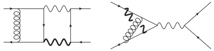
and selected Feynman diagrams are depicted in Figure 1 above.

We are interested in the two-loop master integrals required for the calculation of the $\mathcal{O}(\alpha_{s}\alpha)$ corrections to these processes. In this paper, we restrict ourselves to the subset of these integrals, which involve at most one massive vector boson, $W$ or $Z$, propagating in the loops. We will use the generic symbol $m$ for the vector boson mass. The relevant loop integrals can be indexed using the four integral families shown in Table 1. Integration by parts reduction Tkachov:1981wb ; Chetyrkin:1981qh ; Laporta:2001dd allows us to rewrite any Feynman integral in these families as a linear combination of master integrals. The reductions for this paper were performed with the implementation Reduze 2 vonManteuffel:2012np ; Studerus:2009ye ; Bauer:2000cp ; fermat and we adapt its conventions for the labeling of sectors, etc. An ideal choice for the master integrals will depend on the application and we will discuss suitable options for different applications in the following sections.

Family $\mathrm{A}$ Family $\mathrm{B}$ Family $\mathrm{C}$ Family $\mathrm{D}$
   $k_{1}^{2}$ $k_{2}^{2}$ $k_{1}^{2}$ $k_{2}^{2}$
 $k_{2}^{2}$ $(k_{2}-p_{3})^{2}$ $k_{2}^{2}$ $(k_{2}-p_{3})^{2}$
 $(k_{1}-k_{2})^{2}$ $(k_{2}-p_{1}-p_{2})^{2}$ $(k_{1}-k_{2})^{2}$ $(k_{2}-p_{1}-p_{2})^{2}$
 $(k_{1}-p_{1})^{2}$ $(k_{1}-p_{1})^{2}$ $(k_{1}-p_{1})^{2}$ $(k_{1}-p_{1})^{2}$
 $(k_{2}-p_{1})^{2}$ $(k_{1}-k_{2})^{2}$ $(k_{2}-p_{1})^{2}$ $(k_{1}-k_{2})^{2}$
 $(k_{1}-p_{1}-p_{2})^{2}$ $(k_{1}-k_{2}+p_{2})^{2}$ $(k_{1}-p_{1}-p_{2})^{2}$ $(k_{1}-k_{2}+p_{2})^{2}$
 $(k_{2}-p_{1}-p_{2})^{2}$ $k_{1}^{2}$ $(k_{2}-p_{1}-p_{2})^{2}-m^{2}$ $k_{1}^{2}-m^{2}$
 $(k_{1}-p_{3})^{2}$ $(k_{1}-p_{3})^{2}$ $(k_{1}-p_{3})^{2}$ $(k_{1}-p_{3})^{2}-m^{2}$
 $(k_{2}-p_{3})^{2}$ $(k_{1}-k_{2}+p_{1}+p_{2})^{2}$ $(k_{2}-p_{3})^{2}$ $(k_{1}-k_{2}+p_{1}+p_{2})^{2}$
Table 1: The four integral families used for the two-loop mixed EW-QCD Drell-Yan master integrals with either no massive internal lines or exactly one massive internal line.

3 Analytical Solution from Differential Equations

We employ the method of differential equations to derive analytical solutions for the master integrals. Altogether, we find that we need to consider forty-nine master integrals for the system of differential equations. Some of these integrals are related by a permutation of external legs. They are covered by crossed integral families, which we will denote by an overline (e.g. we write $\mathrm{\accentset{\rule{2.79996pt}{0.8pt}}{F}}$:$x$ for the crossed version of sector $x$ from family $\mathrm{F}$). Note that, because our four-particle integral topologies are naturally a function of the invariants $s$ and $t$ (and never $u=-s-t$), we may without loss of intelligibility suppress all explicit momentum labels; instead, we use directed external lines and explicit function arguments to help clarify our basis integral definitions when necessary. As usual, we use dots to denote doubled propagators, heavy lines to denote massive propagators, and explicitly write all numerator insertions in square brackets. The starting point for the construction of our basis are the following integrals:

f1A:38=[Uncaptioned image](42ϵ)(s)f2A :38=[Uncaptioned image](42ϵ)(t)f3A:99=[Uncaptioned image](42ϵ)(s)formulae-sequencesuperscriptsubscript𝑓1:A3842italic-ϵ[Uncaptioned image]𝑠formulae-sequencesuperscriptsubscript𝑓2: A3842italic-ϵ[Uncaptioned image]𝑡superscriptsubscript𝑓3:A9942italic-ϵ[Uncaptioned image]𝑠\displaystyle f_{1}^{\mathrm{A:38}}=\overset{(4-2\epsilon)}{\includegraphics[valign={m},raise={.3 cm},height=54.2025pt,width=54.2025pt,keepaspectratio]{f1andf2}}(s)\quad f_{2}^{\mathrm{\accentset{\rule{2.79996pt}{0.8pt}}{A}:38}}=\overset{(4-2\epsilon)}{\includegraphics[valign={m},raise={.3 cm},height=54.2025pt,width=54.2025pt,keepaspectratio]{f1andf2}}(t)\quad f_{3}^{\mathrm{A:99}}=\overset{(4-2\epsilon)}{\includegraphics[valign={m},raise={.3 cm},height=75.88481pt,width=75.88481pt,keepaspectratio]{f3andf4}}(s)
f4A :99=[Uncaptioned image](42ϵ)(t)f5A:53=[Uncaptioned image](42ϵ)(s)f6A :53=[Uncaptioned image](42ϵ)(t)formulae-sequencesuperscriptsubscript𝑓4: A9942italic-ϵ[Uncaptioned image]𝑡formulae-sequencesuperscriptsubscript𝑓5:A5342italic-ϵ[Uncaptioned image]𝑠superscriptsubscript𝑓6: A5342italic-ϵ[Uncaptioned image]𝑡\displaystyle f_{4}^{\mathrm{\accentset{\rule{2.79996pt}{0.8pt}}{A}:99}}=\overset{(4-2\epsilon)}{\includegraphics[valign={m},raise={.3 cm},height=75.88481pt,width=75.88481pt,keepaspectratio]{f3andf4}}(t)\quad f_{5}^{\mathrm{A:53}}=\overset{(4-2\epsilon)}{\includegraphics[valign={m},raise={.2 cm},height=58.53632pt,width=58.53632pt,keepaspectratio]{f5andf6}}(s)\quad f_{6}^{\mathrm{\accentset{\rule{2.79996pt}{0.8pt}}{A}:53}}=\overset{(4-2\epsilon)}{\includegraphics[valign={m},raise={.2 cm},height=58.53632pt,width=58.53632pt,keepaspectratio]{f5andf6}}(t)
f7A:174=[Uncaptioned image](42ϵ)(s,t)f8A :174=[Uncaptioned image](42ϵ)(t,s)f9A:182=[Uncaptioned image](42ϵ)(s,t)formulae-sequencesuperscriptsubscript𝑓7:A17442italic-ϵ[Uncaptioned image]𝑠𝑡formulae-sequencesuperscriptsubscript𝑓8: A17442italic-ϵ[Uncaptioned image]𝑡𝑠superscriptsubscript𝑓9:A18242italic-ϵ[Uncaptioned image]𝑠𝑡\displaystyle f_{7}^{\mathrm{A:174}}=\overset{(4-2\epsilon)}{\includegraphics[valign={m},raise={.2 cm},height=58.53632pt,width=58.53632pt,keepaspectratio]{f7}}(s,t)\quad f_{8}^{\mathrm{\accentset{\rule{2.79996pt}{0.8pt}}{A}:174}}=\overset{(4-2\epsilon)}{\includegraphics[valign={m},raise={.2 cm},height=58.53632pt,width=58.53632pt,keepaspectratio]{f8}}(t,s)\quad f_{9}^{\mathrm{A:182}}=\overset{(4-2\epsilon)}{\includegraphics[valign={m},raise={.2 cm},height=58.53632pt,width=58.53632pt,keepaspectratio]{f9}}(s,t)
f10A:247=[Uncaptioned image](42ϵ)(s,t)f11A:247=[Uncaptioned image](42ϵ)[(k2p3)2](s,t)formulae-sequencesuperscriptsubscript𝑓10:A24742italic-ϵ[Uncaptioned image]𝑠𝑡superscriptsubscript𝑓11:A24742italic-ϵ[Uncaptioned image]delimited-[]superscriptsubscript𝑘2subscript𝑝32𝑠𝑡\displaystyle f_{10}^{\mathrm{A:247}}=\overset{(4-2\epsilon)}{\includegraphics[valign={m},raise={.22 cm},height=65.04034pt,width=65.04034pt,keepaspectratio]{f10andf11}}(s,t)\quad f_{11}^{\mathrm{A:247}}=\overset{(4-2\epsilon)}{\includegraphics[valign={m},raise={.22 cm},height=65.04034pt,width=65.04034pt,keepaspectratio]{f10andf11}}\left[(k_{2}-p_{3})^{2}\right](s,t)
f12B:125=[Uncaptioned image](42ϵ)(s)superscriptsubscript𝑓12:B12542italic-ϵ[Uncaptioned image]𝑠\displaystyle f_{12}^{\mathrm{B:125}}=\overset{(4-2\epsilon)}{\includegraphics[valign={m},raise={.3 cm},height=75.88481pt,width=75.88481pt,keepaspectratio]{f12}}(s)
f13C:97=[Uncaptioned image](42ϵ)(s)f14C :97=[Uncaptioned image](42ϵ)(t)f15C:76=[Uncaptioned image](42ϵ)formulae-sequencesuperscriptsubscript𝑓13:C9742italic-ϵ[Uncaptioned image]𝑠formulae-sequencesuperscriptsubscript𝑓14: C9742italic-ϵ[Uncaptioned image]𝑡superscriptsubscript𝑓15:C7642italic-ϵ[Uncaptioned image]\displaystyle f_{13}^{\mathrm{C:97}}=\overset{(4-2\epsilon)}{\includegraphics[valign={m},raise={.3 cm},height=86.72267pt,width=86.72267pt,keepaspectratio]{f13andf14}}(s)\quad f_{14}^{\mathrm{\accentset{\rule{2.79996pt}{0.8pt}}{C}:97}}=\overset{(4-2\epsilon)}{\includegraphics[valign={m},raise={.3 cm},height=86.72267pt,width=86.72267pt,keepaspectratio]{f13andf14}}(t)\quad f_{15}^{\mathrm{C:76}}=\overset{(4-2\epsilon)}{\includegraphics[valign={m},raise={.3 cm},height=21.68231pt,width=21.68231pt,keepaspectratio]{f15}}\quad
f16C:69=[Uncaptioned image](42ϵ)(s)f17C:69=[Uncaptioned image](42ϵ)(s)f18C:99=[Uncaptioned image](42ϵ)(s)formulae-sequencesuperscriptsubscript𝑓16:C6942italic-ϵ[Uncaptioned image]𝑠formulae-sequencesuperscriptsubscript𝑓17:C6942italic-ϵ[Uncaptioned image]𝑠superscriptsubscript𝑓18:C9942italic-ϵ[Uncaptioned image]𝑠\displaystyle f_{16}^{\mathrm{C:69}}=\overset{(4-2\epsilon)}{\includegraphics[valign={m},raise={.3 cm},height=54.2025pt,width=54.2025pt,keepaspectratio]{f16}}(s)\quad f_{17}^{\mathrm{C:69}}=\overset{(4-2\epsilon)}{\includegraphics[valign={m},raise={.3 cm},height=54.2025pt,width=54.2025pt,keepaspectratio]{f17}}(s)\quad f_{18}^{\mathrm{C:99}}=\overset{(4-2\epsilon)}{\includegraphics[valign={m},raise={.3 cm},height=75.88481pt,width=75.88481pt,keepaspectratio]{f18}}(s)
f19C:102=[Uncaptioned image](42ϵ)(s)f20C:78=[Uncaptioned image](42ϵ)(s)f21C:212=[Uncaptioned image](42ϵ)(t)formulae-sequencesuperscriptsubscript𝑓19:C10242italic-ϵ[Uncaptioned image]𝑠formulae-sequencesuperscriptsubscript𝑓20:C7842italic-ϵ[Uncaptioned image]𝑠superscriptsubscript𝑓21:C21242italic-ϵ[Uncaptioned image]𝑡\displaystyle f_{19}^{\mathrm{C:102}}=\overset{(4-2\epsilon)}{\includegraphics[valign={m},raise={.6 cm},height=75.88481pt,width=75.88481pt,keepaspectratio]{f19}}(s)\quad f_{20}^{\mathrm{C:78}}=\overset{(4-2\epsilon)}{\includegraphics[valign={m},raise={.1 cm},height=75.88481pt,width=75.88481pt,keepaspectratio]{f20}}(s)\quad f_{21}^{\mathrm{C:212}}=\overset{(4-2\epsilon)}{\includegraphics[valign={m},raise={.1 cm},height=65.04034pt,width=65.04034pt,keepaspectratio]{f21andf22}}(t)
f22C :212=[Uncaptioned image](42ϵ)(s)f23C:204=[Uncaptioned image](42ϵ)(t)f24C:204=[Uncaptioned image](42ϵ)(t)formulae-sequencesuperscriptsubscript𝑓22: C21242italic-ϵ[Uncaptioned image]𝑠formulae-sequencesuperscriptsubscript𝑓23:C20442italic-ϵ[Uncaptioned image]𝑡superscriptsubscript𝑓24:C20442italic-ϵ[Uncaptioned image]𝑡\displaystyle f_{22}^{\mathrm{\accentset{\rule{2.79996pt}{0.8pt}}{C}:212}}=\overset{(4-2\epsilon)}{\includegraphics[valign={m},raise={.1 cm},height=65.04034pt,width=65.04034pt,keepaspectratio]{f21andf22}}(s)\quad f_{23}^{\mathrm{C:204}}=\overset{(4-2\epsilon)}{\includegraphics[valign={m},raise={.1 cm},height=75.88481pt,width=75.88481pt,keepaspectratio]{f23andf25}}(t)\quad f_{24}^{\mathrm{C:204}}=\overset{(4-2\epsilon)}{\includegraphics[valign={m},raise={.1 cm},height=75.88481pt,width=75.88481pt,keepaspectratio]{f24andf26}}(t)
f25C :204=[Uncaptioned image](42ϵ)(s)f26C :204=[Uncaptioned image](42ϵ)(s)f27C:472=[Uncaptioned image](42ϵ)(t)formulae-sequencesuperscriptsubscript𝑓25: C20442italic-ϵ[Uncaptioned image]𝑠formulae-sequencesuperscriptsubscript𝑓26: C20442italic-ϵ[Uncaptioned image]𝑠superscriptsubscript𝑓27:C47242italic-ϵ[Uncaptioned image]𝑡\displaystyle f_{25}^{\mathrm{\accentset{\rule{2.79996pt}{0.8pt}}{C}:204}}=\overset{(4-2\epsilon)}{\includegraphics[valign={m},raise={.1 cm},height=75.88481pt,width=75.88481pt,keepaspectratio]{f23andf25}}(s)\quad f_{26}^{\mathrm{\accentset{\rule{2.79996pt}{0.8pt}}{C}:204}}=\overset{(4-2\epsilon)}{\includegraphics[valign={m},raise={.1 cm},height=75.88481pt,width=75.88481pt,keepaspectratio]{f24andf26}}(s)\quad f_{27}^{\mathrm{C:472}}=\overset{(4-2\epsilon)}{\includegraphics[valign={m},raise={.2 cm},height=75.88481pt,width=75.88481pt,keepaspectratio]{f27}}(t)
f28C:372=[Uncaptioned image](42ϵ)(t)f29C:244=[Uncaptioned image](42ϵ)(t)f30C :244=[Uncaptioned image](42ϵ)(s)formulae-sequencesuperscriptsubscript𝑓28:C37242italic-ϵ[Uncaptioned image]𝑡formulae-sequencesuperscriptsubscript𝑓29:C24442italic-ϵ[Uncaptioned image]𝑡superscriptsubscript𝑓30: C24442italic-ϵ[Uncaptioned image]𝑠\displaystyle f_{28}^{\mathrm{C:372}}=\overset{(4-2\epsilon)}{\includegraphics[valign={m},raise={.2 cm},height=65.04034pt,width=65.04034pt,keepaspectratio]{f28}}(t)\quad f_{29}^{\mathrm{C:244}}=\overset{(4-2\epsilon)}{\includegraphics[valign={m},raise={.7 cm},height=75.88481pt,width=75.88481pt,keepaspectratio]{f29andf30}}(t)\quad f_{30}^{\mathrm{\accentset{\rule{2.79996pt}{0.8pt}}{C}:244}}=\overset{(4-2\epsilon)}{\includegraphics[valign={m},raise={.7 cm},height=75.88481pt,width=75.88481pt,keepaspectratio]{f29andf30}}(s)\quad
f31C:110=[Uncaptioned image](42ϵ)(s)f32C:220=[Uncaptioned image](42ϵ)(t)f33C :220=[Uncaptioned image](42ϵ)(s)formulae-sequencesuperscriptsubscript𝑓31:C11042italic-ϵ[Uncaptioned image]𝑠formulae-sequencesuperscriptsubscript𝑓32:C22042italic-ϵ[Uncaptioned image]𝑡superscriptsubscript𝑓33: C22042italic-ϵ[Uncaptioned image]𝑠\displaystyle f_{31}^{\mathrm{C:110}}=\overset{(4-2\epsilon)}{\includegraphics[valign={m},raise={.7 cm},height=75.88481pt,width=75.88481pt,keepaspectratio]{f31}}(s)\quad f_{32}^{\mathrm{C:220}}=\overset{(4-2\epsilon)}{\includegraphics[valign={m},raise={.7 cm},height=75.88481pt,width=75.88481pt,keepaspectratio]{f32andf33}}(t)\quad f_{33}^{\mathrm{\accentset{\rule{2.79996pt}{0.8pt}}{C}:220}}=\overset{(4-2\epsilon)}{\includegraphics[valign={m},raise={.7 cm},height=75.88481pt,width=75.88481pt,keepaspectratio]{f32andf33}}(s)
f34C:117=[Uncaptioned image](42ϵ)(s)f35C:117=[Uncaptioned image](42ϵ)(s)f36C:214=[Uncaptioned image](42ϵ)(s,t)formulae-sequencesuperscriptsubscript𝑓34:C11742italic-ϵ[Uncaptioned image]𝑠formulae-sequencesuperscriptsubscript𝑓35:C11742italic-ϵ[Uncaptioned image]𝑠superscriptsubscript𝑓36:C21442italic-ϵ[Uncaptioned image]𝑠𝑡\displaystyle f_{34}^{\mathrm{C:117}}=\overset{(4-2\epsilon)}{\includegraphics[valign={m},raise={.7 cm},height=75.88481pt,width=75.88481pt,keepaspectratio]{f34}}(s)\quad f_{35}^{\mathrm{C:117}}=\overset{(4-2\epsilon)}{\includegraphics[valign={m},raise={.7 cm},height=75.88481pt,width=75.88481pt,keepaspectratio]{f35}}(s)\quad f_{36}^{\mathrm{C:214}}=\overset{(4-2\epsilon)}{\includegraphics[valign={m},raise={.2 cm},height=58.53632pt,width=58.53632pt,keepaspectratio]{f36}}(s,t)
f37C:341=[Uncaptioned image](42ϵ)(s,t)f38C:341=[Uncaptioned image](42ϵ)(s,t)f39C:213=[Uncaptioned image](42ϵ)(s,t)formulae-sequencesuperscriptsubscript𝑓37:C34142italic-ϵ[Uncaptioned image]𝑠𝑡formulae-sequencesuperscriptsubscript𝑓38:C34142italic-ϵ[Uncaptioned image]𝑠𝑡superscriptsubscript𝑓39:C21342italic-ϵ[Uncaptioned image]𝑠𝑡\displaystyle f_{37}^{\mathrm{C:341}}=\overset{(4-2\epsilon)}{\includegraphics[valign={m},raise={.2 cm},height=58.53632pt,width=58.53632pt,keepaspectratio]{f37}}(s,t)\quad f_{38}^{\mathrm{C:341}}=\overset{(4-2\epsilon)}{\includegraphics[valign={m},raise={.2 cm},height=58.53632pt,width=58.53632pt,keepaspectratio]{f38}}(s,t)\quad f_{39}^{\mathrm{C:213}}=\overset{(4-2\epsilon)}{\includegraphics[valign={m},raise={.2 cm},height=58.53632pt,width=58.53632pt,keepaspectratio]{f39}}(s,t)
f40C:213=[Uncaptioned image](42ϵ)(s,t)f41C:374=[Uncaptioned image](42ϵ)(s,t)f42C:246=[Uncaptioned image](42ϵ)(s,t)formulae-sequencesuperscriptsubscript𝑓40:C21342italic-ϵ[Uncaptioned image]𝑠𝑡formulae-sequencesuperscriptsubscript𝑓41:C37442italic-ϵ[Uncaptioned image]𝑠𝑡superscriptsubscript𝑓42:C24642italic-ϵ[Uncaptioned image]𝑠𝑡\displaystyle f_{40}^{\mathrm{C:213}}=\overset{(4-2\epsilon)}{\includegraphics[valign={m},raise={.2 cm},height=58.53632pt,width=58.53632pt,keepaspectratio]{f40}}(s,t)\quad f_{41}^{\mathrm{C:374}}=\overset{(4-2\epsilon)}{\includegraphics[valign={m},raise={.45 cm},height=65.04034pt,width=65.04034pt,keepaspectratio]{f41}}(s,t)\quad f_{42}^{\mathrm{C:246}}=\overset{(4-2\epsilon)}{\includegraphics[valign={m},raise={.45 cm},height=65.04034pt,width=65.04034pt,keepaspectratio]{f42}}(s,t)
f43C:245=[Uncaptioned image](42ϵ)(s,t)f44C:245=[Uncaptioned image](42ϵ)(s,t)formulae-sequencesuperscriptsubscript𝑓43:C24542italic-ϵ[Uncaptioned image]𝑠𝑡superscriptsubscript𝑓44:C24542italic-ϵ[Uncaptioned image]𝑠𝑡\displaystyle f_{43}^{\mathrm{C:245}}=\overset{(4-2\epsilon)}{\includegraphics[valign={m},raise={.45 cm},height=65.04034pt,width=65.04034pt,keepaspectratio]{f43}}(s,t)\quad\quad f_{44}^{\mathrm{C:245}}=\overset{(4-2\epsilon)}{\includegraphics[valign={m},raise={.45 cm},height=65.04034pt,width=65.04034pt,keepaspectratio]{f44}}(s,t)
f45C:247=[Uncaptioned image](42ϵ)(s,t)f46C:247=[Uncaptioned image](42ϵ)[(k2p3)2](s,t)formulae-sequencesuperscriptsubscript𝑓45:C24742italic-ϵ[Uncaptioned image]𝑠𝑡superscriptsubscript𝑓46:C24742italic-ϵ[Uncaptioned image]delimited-[]superscriptsubscript𝑘2subscript𝑝32𝑠𝑡\displaystyle f_{45}^{\mathrm{C:247}}=\overset{(4-2\epsilon)}{\includegraphics[valign={m},raise={.22 cm},height=65.04034pt,width=65.04034pt,keepaspectratio]{f45andf46}}(s,t)\quad f_{46}^{\mathrm{C:247}}=\overset{(4-2\epsilon)}{\includegraphics[valign={m},raise={.22 cm},height=65.04034pt,width=65.04034pt,keepaspectratio]{f45andf46}}\left[(k_{2}-p_{3})^{2}\right](s,t)
f47D:341=[Uncaptioned image](42ϵ)(s)f48D:117=[Uncaptioned image](42ϵ)(s)formulae-sequencesuperscriptsubscript𝑓47:D34142italic-ϵ[Uncaptioned image]𝑠superscriptsubscript𝑓48:D11742italic-ϵ[Uncaptioned image]𝑠\displaystyle f_{47}^{\mathrm{D:341}}=\overset{(4-2\epsilon)}{\includegraphics[valign={m},raise={.3 cm},height=75.88481pt,width=75.88481pt,keepaspectratio]{f47}}(s)\quad\quad f_{48}^{\mathrm{D:117}}=\overset{(4-2\epsilon)}{\includegraphics[valign={m},raise={.7 cm},height=75.88481pt,width=75.88481pt,keepaspectratio]{f48}}(s)
f49D:125=[Uncaptioned image](42ϵ)[(k1k2+p1+p2)2](s).superscriptsubscript𝑓49:D12542italic-ϵ[Uncaptioned image]delimited-[]superscriptsubscript𝑘1subscript𝑘2subscript𝑝1subscript𝑝22𝑠\displaystyle f_{49}^{\mathrm{D:125}}=\overset{(4-2\epsilon)}{\includegraphics[valign={m},raise={.22 cm},height=65.04034pt,width=65.04034pt,keepaspectratio]{f49}}\left[(k_{1}-k_{2}+p_{1}+p_{2})^{2}\right](s). (6)

Building upon these definitions, we construct a convenient basis of integrals for the method of differential equations along the lines discussed in reference Gehrmann:2014bfa :222 We would like to point out further recent work on the analysis of master integrals and the construction of a normal form basis Lee:2013hzt ; Argeri:2014qva ; Lee:2014ioa ; Tancredi:2015pta ; Ablinger:2015tua ; Ita:2015tya ; Larsen:2015ped ; Primo:2016ebd ; Meyer:2016slj ; Georgoudis:2016wff ; Prausa:2017ltv ; Gituliar:2017vzm .

$\displaystyle m_{1}=\epsilon^{2}sf_{1}^{\mathrm{A:38}}\quad m_{2}=\epsilon^{2}tf_{2}^{\mathrm{\accentset{\rule{2.79996pt}{0.8pt}}{A}:38}}\quad m_{3}=\epsilon^{2}s^{2}f_{3}^{\mathrm{A:99}}\quad m_{4}=\epsilon^{2}t^{2}f_{4}^{\mathrm{\accentset{\rule{2.79996pt}{0.8pt}}{A}:99}}\quad m_{5}=\epsilon^{3}sf_{5}^{\mathrm{A:53}}$
$\displaystyle m_{6}=\epsilon^{3}tf_{6}^{\mathrm{\accentset{\rule{2.79996pt}{0.8pt}}{A}:53}}\quad m_{7}=\epsilon^{3}stf_{7}^{\mathrm{A:174}}\quad m_{8}=\epsilon^{3}stf_{8}^{\mathrm{\accentset{\rule{2.79996pt}{0.8pt}}{A}:174}}\quad m_{9}=\epsilon^{4}(s+t)f_{9}^{\mathrm{A:182}}$
$\displaystyle m_{10}=\epsilon^{4}s^{2}tf_{10}^{\mathrm{A:247}}\quad m_{11}=\epsilon^{4}s^{2}f_{11}^{\mathrm{A:247}}\quad m_{12}=\epsilon^{4}s^{2}f_{12}^{\mathrm{B:125}}\quad m_{13}=\epsilon^{2}sf_{1}^{\mathrm{A:38}}$
$\displaystyle m_{14}=\epsilon^{2}tf_{2}^{\mathrm{\accentset{\rule{2.79996pt}{0.8pt}}{A}:38}}\quad m_{15}=\epsilon^{2}sf_{13}^{\mathrm{C:97}}\quad m_{16}=\epsilon^{2}tf_{14}^{\mathrm{\accentset{\rule{2.79996pt}{0.8pt}}{C}:97}}\quad m_{17}=\epsilon(1-\epsilon)m^{2}f_{15}^{\mathrm{C:76}}$
$\displaystyle m_{18}=\epsilon^{2}sf_{16}^{\mathrm{C:69}}\quad m_{19}=2\epsilon^{2}(s-m^{2})f_{16}^{\mathrm{C:69}}+\epsilon^{2}(s-m^{2})f_{17}^{\mathrm{C:69}}\quad m_{20}=\epsilon^{2}s^{2}f_{3}^{\mathrm{A:99}}$
$\displaystyle m_{21}=\epsilon^{2}t^{2}f_{4}^{\mathrm{\accentset{\rule{2.79996pt}{0.8pt}}{A}:99}}\quad m_{22}=\epsilon^{3}sf_{5}^{\mathrm{A:53}}\quad m_{23}=\epsilon^{3}tf_{6}^{\mathrm{\accentset{\rule{2.79996pt}{0.8pt}}{A}:53}}\quad m_{24}=\epsilon^{2}s^{2}f_{18}^{\mathrm{C:99}}$
$\displaystyle m_{25}=\frac{\epsilon^{2}s\Big{(}s(1-5\epsilon)-m^{2}(1-3\epsilon)\Big{)}}{4(1-3\epsilon)(s-m^{2})}f_{1}^{\mathrm{A:38}}-\frac{\epsilon(1-\epsilon)m^{4}}{2(s-m^{2})}f_{15}^{\mathrm{C:76}}+\frac{\epsilon^{2}(1-2\epsilon)^{2}}{s-m^{2}}f_{19}^{\mathrm{C:102}}$
$\displaystyle m_{26}=\epsilon^{3}sf_{20}^{\mathrm{C:78}}\quad m_{27}=\epsilon^{3}tf_{21}^{\mathrm{C:212}}\quad m_{28}=\epsilon^{3}sf_{22}^{\mathrm{\accentset{\rule{2.79996pt}{0.8pt}}{C}:212}}\quad m_{29}=\epsilon^{3}tf_{23}^{\mathrm{C:204}}\quad m_{30}=\epsilon^{3}tf_{24}^{\mathrm{C:204}}$
$\displaystyle m_{31}=\epsilon^{3}tf_{25}^{\mathrm{\accentset{\rule{2.79996pt}{0.8pt}}{C}:204}}\quad m_{32}=\epsilon^{3}tf_{26}^{\mathrm{\accentset{\rule{2.79996pt}{0.8pt}}{C}:204}}\quad m_{33}=\epsilon^{3}stf_{7}^{\mathrm{A:174}}\quad m_{34}=\epsilon^{3}stf_{8}^{\mathrm{\accentset{\rule{2.79996pt}{0.8pt}}{A}:174}}$
$\displaystyle m_{35}=\epsilon^{4}(s+t)f_{9}^{\mathrm{A:182}}\quad m_{36}=\epsilon^{3}t^{2}f_{27}^{\mathrm{C:472}}\quad m_{37}=\epsilon^{3}m^{2}tf_{28}^{\mathrm{C:372}}\quad m_{38}=\epsilon^{3}m^{2}tf_{29}^{\mathrm{C:244}}$
$\displaystyle m_{39}=\epsilon^{3}m^{2}sf_{30}^{\mathrm{\accentset{\rule{2.79996pt}{0.8pt}}{C}:244}}\quad m_{40}=\epsilon^{4}sf_{31}^{\mathrm{C:110}}\quad m_{41}=\epsilon^{3}m^{2}tf_{32}^{\mathrm{C:220}}\quad m_{42}=\epsilon^{3}m^{2}sf_{33}^{\mathrm{\accentset{\rule{2.79996pt}{0.8pt}}{C}:220}}$
$\displaystyle m_{43}=\epsilon^{3}m^{2}sf_{34}^{\mathrm{C:117}}\quad m_{44}=\epsilon^{3}s^{2}f_{35}^{\mathrm{C:117}}\quad m_{45}=\epsilon^{3}(s-m^{2})tf_{36}^{\mathrm{C:214}}\quad m_{46}=\epsilon^{3}(1-2\epsilon)tf_{37}^{\mathrm{C:341}}$
$\displaystyle m_{47}=3\epsilon^{3}(1-2\epsilon)m^{2}f_{37}^{\mathrm{C:341}}+\epsilon^{2}(1-2\epsilon)m^{2}(m^{2}+t)f_{38}^{\mathrm{C:341}}\quad m_{48}=\epsilon^{4}(s+t)f_{39}^{\mathrm{C:213}}\quad$
$\displaystyle m_{49}=\epsilon^{3}m^{2}(s+t)f_{40}^{\mathrm{C:213}}\quad m_{50}=\epsilon^{3}(1-2\epsilon)(s-m^{2})tf_{41}^{\mathrm{C:374}}\quad m_{51}=\epsilon^{4}(st-m^{2}(s+t))f_{42}^{\mathrm{C:246}}$
$\displaystyle m_{52}=\epsilon^{4}stf_{43}^{\mathrm{C:245}}\quad m_{53}=2\epsilon^{4}m^{2}sf_{43}^{\mathrm{C:245}}+\epsilon^{3}m^{2}s(m^{2}+t)f_{44}^{\mathrm{C:245}}\quad m_{54}=\epsilon^{4}s(s-m^{2})tf_{45}^{\mathrm{C:247}}$
$\displaystyle m_{55}=\epsilon^{4}s^{2}f_{46}^{\mathrm{C:247}}\quad m_{56}=\epsilon^{3}(1-2\epsilon)sf_{47}^{\mathrm{D:341}}\quad m_{57}=\epsilon^{4}sf_{48}^{\mathrm{D:117}}\quad m_{58}=\epsilon^{4}sf_{49}^{\mathrm{D:125}}.$ (7)

Note that these definitions repeat nine massless integrals to allow for an independent treatment of the differential equations for the massless integrals, $m_{1},\ldots,m_{12}$, and the one-mass integrals, $m_{13},\ldots,m_{58}$. We employ the integration measure

$$\left(\frac{\Gamma(1-\epsilon)s^{\epsilon}}{i\pi^{2-\epsilon}}\right)^{2}\int{\rm d}^{4-2\epsilon}k_{1}\int{\rm d}^{4-2\epsilon}k_{2}$$ (8)

with $\epsilon=(4-d)/2$, which renders our integrals $m_{i}$ functions of the dimensionless variables

$$x=\frac{-t}{-s}\qquad{\rm and}\qquad y=\frac{m^{2}}{-s}$$ (9)

only.

In this basis, we obtain a system of differential equations in normal form Kotikov:2010gf ; Henn:2013pwa ; Henn:2013tua for the vector $\vec{m}=(m_{i})$,

$$\mathrm{d}\vec{m}(\epsilon,x,y)=\epsilon\sum_{k}\mathrm{d}\ln\big{(}l_{k}(x,y)\big{)}\,A^{(k)}\vec{m}(\epsilon,x,y)$$ (10)

with the letters $l_{k}(x,y)$ of the symbol alphabet

$$\{l_{1},\ldots,l_{7}\}=\left\{x,1+x,y,1+y,1-y,x-y,x+y+xy\right\}$$ (11)

and matrices $A^{(k)}$ of rational numbers.

Expanding the masters integrals $m_{i}$ about $\epsilon=0$, the differential equations fully decouple and can be integrated order-by-order in $\epsilon$ in terms of multiple polylogarithms. The alphabet is linear in both variables, which implies that the integration path can be chosen along the $x$ and $y$ axis, resulting in an expression written in terms of Goncharov $G$ functions with either $x$ or $y$ in the final argument. This representation can introduce spurious singularities and therefore may not be optimal for numerical evaluations Gehrmann:2015ora .

Instead, one can employ $\operatorname{Li}$ functions of fewer but possibly more involved arguments. Recently, it has been demonstrated explicitly that $\ln$, $\operatorname{Li}_{2}$, $\operatorname{Li}_{3}$, $\operatorname{Li}_{4}$, and $\operatorname{Li}_{2,2}$ functions are sufficient to reduce a general $G$ function of at most weight four Frellesvig:2016ske . In order to arrive at real-valued functions with a convergent power series representation in a specific region of phase space, it can be useful to allow for $\operatorname{Li}_{2,1}$ functions as well. A representation written in terms of such functions can be obtained either by recasting a solution written in terms of $G$ functions or by directly integrating the differential equations via an ansatz built out of the required functions. We perform these calculations using in-house routines based on the symbol and coproduct calculus Goncharov:2005sla ; Brown:2011ik ; Duhr:2011zq ; Duhr:2012fh .

Note that, for phenomenological applications, we are interested in the solutions of our integrals through to weight four. In the next section, however, we consider alternative bases of master integrals for the purpose of numerical evaluation which partially involve weight five functions at the $\epsilon$ order required for physics applications. In order to validate our numerical analysis of the solution, we therefore find it useful to obtain results through to weight five.

We construct an ansatz for our solutions in terms of the functions

$$\ln,\quad\operatorname{Li}_{2},\quad\operatorname{Li}_{3},\quad\operatorname{Li}_{2,1},\quad\operatorname{Li}_{4},\quad\operatorname{Li}_{2,2},\quad\operatorname{Li}_{5},\quad\operatorname{Li}_{3,2},\quad\operatorname{Li}_{2,2,1}$$ (12)

using the Duhr-Gangl-Rhodes algorithm Duhr:2011zq . We require the symbol of each function to not introduce letters beyond those already present in our differential equation (10) and we construct suitable power products of our letters (11) accordingly. For the arguments of the logarithms $\ln$ we choose

$$\{-l_{1},l_{2},-l_{3},l_{4},l_{5},-l_{6},-l_{7}\}.$$

As admissible arguments for the classical polylogarithms $\operatorname{Li}_{n}$, we obtain the following sixty-six power products of letters

$\displaystyle\bigg{\{}$ $\displaystyle-l_{1},l_{2},-l_{3},l_{3},l_{4},l_{5},-l_{7},-\frac{1}{l_{7}},\frac{1}{l_{5}},\frac{1}{l_{4}},-\frac{1}{l_{3}},\frac{1}{l_{3}},\frac{1}{l_{2}},-\frac{1}{l_{1}},\frac{l_{1}}{l_{7}},\frac{l_{1}}{l_{6}},\frac{l_{1}}{l_{3}},\frac{l_{1}}{l_{2}},l_{2}l_{4},\frac{l_{2}}{l_{6}},\frac{l_{2}}{l_{4}},l_{3}^{2},\frac{l_{3}}{l_{7}},$
$\displaystyle-\frac{l_{3}}{l_{6}},-\frac{l_{3}}{l_{5}},\frac{l_{3}}{l_{4}},l_{4}l_{5},-\frac{l_{4}}{l_{6}},-\frac{l_{6}}{l_{4}},\frac{1}{l_{4}l_{5}},\frac{l_{4}}{l_{3}},-\frac{l_{5}}{l_{3}},-\frac{l_{6}}{l_{3}},\frac{l_{7}}{l_{3}},\frac{1}{l_{3}^{2}},\frac{l_{4}}{l_{2}},\frac{l_{6}}{l_{2}},\frac{1}{l_{2}l_{4}},\frac{l_{2}}{l_{1}},\frac{l_{3}}{l_{1}},\frac{l_{6}}{l_{1}},\frac{l_{7}}{l_{1}},\frac{l_{1}l_{4}}{l_{7}},$
$\displaystyle\frac{l_{1}l_{4}}{l_{6}},-\frac{l_{1}l_{4}}{l_{3}},-\frac{l_{1}}{l_{2}l_{3}},\frac{l_{2}l_{3}}{l_{7}},-\frac{l_{2}l_{3}}{l_{6}},\frac{l_{2}l_{4}}{l_{7}},\frac{l_{7}}{l_{2}l_{4}},-\frac{l_{6}}{l_{2}l_{3}},\frac{l_{7}}{l_{2}l_{3}},-\frac{l_{2}l_{3}}{l_{1}},-\frac{l_{3}}{l_{1}l_{4}},\frac{l_{6}}{l_{1}l_{4}},\frac{l_{7}}{l_{1}l_{4}},\frac{l_{1}l_{4}}{l_{2}l_{3}},-\frac{l_{3}^{2}}{l_{4}l_{5}},$
$\displaystyle-\frac{l_{4}l_{5}}{l_{3}^{2}},\frac{l_{2}l_{3}}{l_{1}l_{4}},\frac{l_{1}^{2}l_{4}}{l_{6}l_{7}},-\frac{l_{2}l_{3}^{2}}{l_{6}l_{7}},-\frac{l_{6}l_{7}}{l_{2}l_{3}^{2}},\frac{l_{6}l_{7}}{l_{1}^{2}l_{4}},\frac{l_{1}^{2}l_{4}}{l_{2}l_{3}^{2}},\frac{l_{2}l_{3}^{2}}{l_{1}^{2}l_{4}}\bigg{\}}$ (13)

which have the property that not only the argument $z$ but also $1-z$ factorize over the original symbol alphabet. Extending this set by the argument $1$, forming pairs and selecting those pairs $(z_{1},z_{2})$, for which $1-z_{1}z_{2}$ factorizes over the alphabet, gives us 618 admissible arguments for $\operatorname{Li}_{2,1}$, $\operatorname{Li}_{2,2}$, and $\operatorname{Li}_{3,2}$ functions which we do not list here for the sake of brevity. Similarly, we find 3342 admissible triples $(z_{1},z_{2},z_{3})$ as arguments for our $\operatorname{Li}_{2,2,1}$ functions. While we have no proof that $\operatorname{Li}_{2,2,1}$ functions are strictly required, we were successful in constructing the genuine weight five part of the solution only when including them in addition to $\operatorname{Li}_{3,2}$ and $\operatorname{Li}_{5}$ functions. This observation is independent of further constraints to be described below, which motivate the inclusion of $\operatorname{Li}_{2,1}$ functions.

Not all of these functions are needed and we formulate further objectives for our functional basis. We prefer functions which are real-valued for physical kinematics

$$-1<x<0,\quad-\infty<y<0\,.$$ (14)

This requirement is the reason why we include $\operatorname{Li}_{2,1}$ functions in our basis. In addition to requiring real-valuedness, we prefer functions which possess a convergent power series representation. Insisting upon such a representation automatically avoids additional manipulations which might otherwise be necessary to carry out numerical evaluations.

Indeed, we find that it is possible to use functions which are real-valued over the entire physical region of the phase space with a single important exception. The letter $l_{4}=1+y$ changes sign at $s=m^{2}$ and the functional form of our results will change in this region if we insist upon separating real and imaginary parts explicitly. This, however, is to be expected because there is a physical singularity at the point $s=m^{2}$, which would be regulated by the width of the massive vector boson inside the loop. Our solution, in fact, contains just a single function which is sensitive to the cut starting at $y=-1$:

$\displaystyle\ln(l_{4})$ $\displaystyle\text{for~{}}y>-1$ (15)
$\displaystyle\ln(-l_{4})+i\pi$ $\displaystyle\text{for~{}}y<-1.$ (16)

In contrast, no logarithms of the letter $l_{6}=x-y$ appear in our results and all other elements of our functional basis which depend of $l_{6}$ are real-valued for both $x>y$ and $x<y$.

Employing our functional basis, we construct an ansatz for the solution and match it against the differential equations (10). We employ regularity conditions and require real-valuedness in the Euclidean domain to fix the integration constants. In addition, we calculated $f_{1}^{\mathrm{A:38}}$, $f_{3}^{\mathrm{A:99}}$, $f_{5}^{\mathrm{A:53}}$, $f_{13}^{\mathrm{C:97}}$, $f_{15}^{\mathrm{C:76}}$, $f_{16}^{\mathrm{C:69}}$, $f_{18}^{\mathrm{C:99}}$, $f_{27}^{\mathrm{C:472}}$, and $f_{29}^{\mathrm{C:244}}$ explicitly from Feynman parameters to all orders in $\epsilon$. Most of these integrals are completely straightforward to evaluate. Some, such as

$\displaystyle f_{29}^{\mathrm{C:244}}$ $\displaystyle=\frac{s^{2\epsilon}\left(m^{2}\right)^{-2-2\epsilon}\Gamma(1-2\epsilon)\Gamma^{4}(1-\epsilon)\Gamma(2+\epsilon)\Gamma(1+2\epsilon)}{2\,\epsilon^{3}\Gamma(2-\epsilon)\Gamma(-2\epsilon)}{}_{3}F_{2}\left(1,1,2+\epsilon;2,2-\epsilon;\frac{-t}{m^{2}}\right)$
$\displaystyle-\frac{s^{2\epsilon}(-t)^{-1-2\epsilon}\Gamma^{5}(1-\epsilon)\Gamma(1+2\epsilon)}{2\,m^{2}\epsilon^{3}\Gamma(1-3\epsilon)}{}_{3}F_{2}\left(1,-2\epsilon,1-\epsilon;1-2\epsilon,1-3\epsilon;\frac{-t}{m^{2}}\right)$ (17)

turn out to be a bit more non-trivial.

As an additional sanity check, we found it convenient in some cases to look at asymptotic expansions of integrals in particular limits in order to explicitly confirm their scaling behavior. For this purpose, we found the Mathematica package asy.m Jantzen:2012mw to be extremely useful. For the convenience of the reader, we provide our analytical solutions through to weight four in the ancillary files sol-phys-AB.m and sol-phys-CD.m on arXiv.org.

4 Numerical Analysis

In an effort to check an analytical calculation such as the one presented in the previous section, it is desirable to numerically evaluate the loop integrals with an independent method. In other cases, a numerical evaluation might even be the method of choice, e.g. if it is not clear how to evaluate the integrals analytically. A standard method for numerical evaluation is sector decomposition and one might think that it is straightforward to numerically check the integrals $f_{i}$ in (6) using this approach. Unfortunately, this is not the case. Specifically, for double box integrals with additional numerators or dotted propagators we often encountered cases where none of the available software packages is able to provide reliable results. In some cases, issues related to the presence of problematic singularity structures in the integrand can be tracked down and, with dedicated effort, cured Borowka:2013cma . For what concerns the two-loop mixed EW-QCD topologies considered in this paper, the most challenging cases for the code are seven-line integrals which have $\epsilon^{-4}$ poles and doubled propagator denominators.

As discussed in earlier work by the authors and Erik Panzer vonManteuffel:2014qoa ; vonManteuffel:2015gxa , it is possible to employ a basis of finite Feynman integrals defined by allowing for higher-dimensional integrals with potentially higher powers of the propagator denominators to extract all poles in $\epsilon$ analytically before performing any numerical integrations.333Let us remind the reader that, due to the principle of analytical continuation, the existence of an on-shell Euclidean region for all integrals guarantees that our procedure applies equally well to all integrals when physical kinematics is considered. The change of basis is performed with integration by parts reductions, whose computational complexity is non-negligible but still lower than that of the reductions for the amplitude. This is true both for the processes discussed in this work and for all other phenomenologically relevant problems which we have studied.

The finite integrals could, in principle, be evaluated by direct numerical integration. However, their integrands may still contain structures which spoil the convergence of the numerical integrations, such as integrable but large variations near the boundaries. In our experiments with a limited number of Euclidean integrals, we find that an additional sector decomposition step improves the performance of the evaluation. Furthermore, handling branch cuts requires a dedicated treatment for physical kinematics. We therefore find it convenient to employ existing sector decomposition programs for the numerical integration of our finite integrals.

We employ the sector decomposition program SecDec 3 to evaluate our two-loop topologies using either conventional or finite master integrals. As is apparent from Table LABEL:tab:mixedDYnums, working with a basis of finite integrals improves the numerical performance tremendously. Let us now explain in more detail how we used the code to produce Table LABEL:tab:mixedDYnums. Although we made a good effort to use the program in an appropriate way, it is certainly possible that other researchers might manage to produce better results in less time. However, we at least took care to use identical program settings and hardware while carrying out our numerical studies of the conventional and finite integral bases.444We followed the recommendations given in Borowka:2015mxa as much as possible, using, for example, their new sector decomposition strategy G2 and Mathematica 9.0.1 for all of our calculations. Using this version of Mathematica avoided some parallelization issues encountered with versions 8 or 10 in our experiments.

Altogether, we ran for roughly sixty days on the four cores of a i7-4940MX processor. For our finite integral evaluations, just over an hour was required; the excessive run time is due to the fact that, in spite of allowing the VEGAS routine Lepage:1977sw provided by CUBA Hahn:2004fe to sample up to $5\times 10^{8}$ points, numerous conventional basis integrals failed to achieve the very modest goal of $\mathtt{epsrel}=1\times 10^{-2}$ and $\mathtt{epsabs}=1\times 10^{-4}$ at the physical phase space point $p=\{s\rightarrow 17,t\rightarrow-7,m^{2}\rightarrow 6241/1681\}$. Analytical expressions for the finite basis integrals were obtained by using the explicit connection between the finite integral basis and the normal form integral basis. We found good agreement in all cases. At worst, we recorded a fractional difference of $6\times 10^{-3}$ at weight four between our exact results evaluated at $p$ and the numerical results output by the program. The average relative accuracy at weight four was found to be $9\times 10^{-4}$, quite acceptable given our modest accuracy goal.

Due to the fact that there is a substantial loss of precision in rotating from the finite integral basis to the normal form integral basis, we found that our initial $\mathtt{epsrel}=1\times 10^{-2}$ and $\mathtt{epsabs}=1\times 10^{-4}$ run of SecDec 3 did not allow us to directly check the normal form basis to similar part per mille precision. To achieve this, we had to carry out a second, higher precision run of the program with $\mathtt{epsrel}=1\times 10^{-4}$ and $\mathtt{epsabs}=1\times 10^{-8}$, which took roughly eleven days of run time. Let us stress again that it would be hopeless to attempt this exercise using the conventional integral basis.

Table 2: Numerical performance of finite and conventional integral bases for two-loop mixed EW-QCD corrections to Drell-Yan lepton production in the physical region using SecDec 3. For each integral in the above, the run time is given in seconds and the fractional difference from the analytical solution is given for the expansion coefficient which first gives rise to weight four multiple polylogarithms. In the final row of the table, total run times and worst-case relative accuracies are recorded for both integral bases.
[Uncaptioned image](82ϵ)(s)82italic-ϵ[Uncaptioned image]𝑠\overset{(8-2\epsilon)}{\vbox{\hbox{\includegraphics[scale={.2}]{finf1andf2}}}}(s) $4~{}\mathrm{s}$ $3.17\times 10^{-4}$ [Uncaptioned image](42ϵ)(s)42italic-ϵ[Uncaptioned image]𝑠\overset{(4-2\epsilon)}{\vbox{\hbox{\includegraphics[scale={.2}]{cornerf1andf2}}}}(s) $4~{}\mathrm{s}$ $3.42\times 10^{-3}$
[Uncaptioned image](82ϵ)(t)82italic-ϵ[Uncaptioned image]𝑡\overset{(8-2\epsilon)}{\vbox{\hbox{\includegraphics[scale={.2}]{finf1andf2}}}}(t) $4~{}\mathrm{s}$ $8.39\times 10^{-7}$ [Uncaptioned image](42ϵ)(t)42italic-ϵ[Uncaptioned image]𝑡\overset{(4-2\epsilon)}{\vbox{\hbox{\includegraphics[scale={.2}]{cornerf1andf2}}}}(t) $4~{}\mathrm{s}$ $1.40\times 10^{-6}$
[Uncaptioned image](62ϵ)(s)62italic-ϵ[Uncaptioned image]𝑠\overset{(6-2\epsilon)}{\vbox{\hbox{\includegraphics[scale={.2}]{finf3andf4}}}}(s) $11~{}\mathrm{s}$ $3.77\times 10^{-4}$ [Uncaptioned image](42ϵ)(s)42italic-ϵ[Uncaptioned image]𝑠\overset{(4-2\epsilon)}{\vbox{\hbox{\includegraphics[scale={.2}]{cornerf3andf4}}}}(s) $48~{}\mathrm{s}$ $2.11\times 10^{-3}$
[Uncaptioned image](62ϵ)(t)62italic-ϵ[Uncaptioned image]𝑡\overset{(6-2\epsilon)}{\vbox{\hbox{\includegraphics[scale={.2}]{finf3andf4}}}}(t) $4~{}\mathrm{s}$ $1.33\times 10^{-5}$ [Uncaptioned image](42ϵ)(t)42italic-ϵ[Uncaptioned image]𝑡\overset{(4-2\epsilon)}{\vbox{\hbox{\includegraphics[scale={.2}]{cornerf3andf4}}}}(t) $12~{}\mathrm{s}$ $4.98\times 10^{-5}$
[Uncaptioned image](102ϵ)(s)102italic-ϵ[Uncaptioned image]𝑠\overset{(10-2\epsilon)}{\vbox{\hbox{\includegraphics[scale={.2}]{finf5andf6}}}}(s) $5~{}\mathrm{s}$ $1.40\times 10^{-3}$ [Uncaptioned image](42ϵ)(s)42italic-ϵ[Uncaptioned image]𝑠\overset{(4-2\epsilon)}{\vbox{\hbox{\includegraphics[scale={.2}]{cornerf5andf6}}}}(s) $21~{}\mathrm{s}$ $3.31\times 10^{-3}$
[Uncaptioned image](102ϵ)(t)102italic-ϵ[Uncaptioned image]𝑡\overset{(10-2\epsilon)}{\vbox{\hbox{\includegraphics[scale={.2}]{finf5andf6}}}}(t) $4~{}\mathrm{s}$ $7.20\times 10^{-5}$ [Uncaptioned image](42ϵ)(t)42italic-ϵ[Uncaptioned image]𝑡\overset{(4-2\epsilon)}{\vbox{\hbox{\includegraphics[scale={.2}]{cornerf5andf6}}}}(t) $5~{}\mathrm{s}$ $1.11\times 10^{-5}$
[Uncaptioned image](62ϵ)(s,t)62italic-ϵ[Uncaptioned image]𝑠𝑡\overset{(6-2\epsilon)}{\vbox{\hbox{\includegraphics[scale={.2}]{finf7}}}}(s,t) $13~{}\mathrm{s}$ $5.76\times 10^{-3}$ [Uncaptioned image](42ϵ)(s,t)42italic-ϵ[Uncaptioned image]𝑠𝑡\overset{(4-2\epsilon)}{\vbox{\hbox{\includegraphics[scale={.2}]{cornerf7}}}}(s,t) $48~{}\mathrm{s}$ $4.56\times 10^{-3}$
[Uncaptioned image](62ϵ)(t,s)62italic-ϵ[Uncaptioned image]𝑡𝑠\overset{(6-2\epsilon)}{\vbox{\hbox{\includegraphics[scale={.2}]{finf8}}}}(t,s) $31~{}\mathrm{s}$ $3.31\times 10^{-3}$ [Uncaptioned image](42ϵ)(t,s)42italic-ϵ[Uncaptioned image]𝑡𝑠\overset{(4-2\epsilon)}{\vbox{\hbox{\includegraphics[scale={.2}]{cornerf8}}}}(t,s) $37~{}\mathrm{s}$ $2.74\times 10^{-3}$
[Uncaptioned image](102ϵ)(s,t)102italic-ϵ[Uncaptioned image]𝑠𝑡\overset{(10-2\epsilon)}{\vbox{\hbox{\includegraphics[scale={.2}]{finf9}}}}(s,t) $8~{}\mathrm{s}$ $6.70\times 10^{-4}$ [Uncaptioned image](42ϵ)(s,t)42italic-ϵ[Uncaptioned image]𝑠𝑡\overset{(4-2\epsilon)}{\vbox{\hbox{\includegraphics[scale={.2}]{cornerf9}}}}(s,t) $8~{}\mathrm{s}$ $1.27\times 10^{-3}$
[Uncaptioned image](62ϵ)(s,t)62italic-ϵ[Uncaptioned image]𝑠𝑡\overset{(6-2\epsilon)}{\vbox{\hbox{\includegraphics[scale={.2}]{finf10}}}}(s,t) $212~{}\mathrm{s}$ $3.44\times 10^{-3}$ [Uncaptioned image](42ϵ)(s,t)42italic-ϵ[Uncaptioned image]𝑠𝑡\overset{(4-2\epsilon)}{\vbox{\hbox{\includegraphics[scale={.2}]{cornerf10}}}}(s,t) $17503~{}\mathrm{s}$ $3.59\times 10^{-3}$
[Uncaptioned image](62ϵ)(s,t)62italic-ϵ[Uncaptioned image]𝑠𝑡\overset{(6-2\epsilon)}{\vbox{\hbox{\includegraphics[scale={.2}]{finf11}}}}(s,t) $197~{}\mathrm{s}$ $1.84\times 10^{-4}$ [Uncaptioned image](42ϵ)(s,t)42italic-ϵ[Uncaptioned image]𝑠𝑡\overset{(4-2\epsilon)}{\vbox{\hbox{\includegraphics[scale={.2}]{cornerf11}}}}(s,t) $1337751~{}\mathrm{s}$ $.263$
[Uncaptioned image](82ϵ)(s)82italic-ϵ[Uncaptioned image]𝑠\overset{(8-2\epsilon)}{\vbox{\hbox{\includegraphics[scale={.2}]{finf12}}}}(s) $8~{}\mathrm{s}$ $4.18\times 10^{-3}$ [Uncaptioned image](42ϵ)(s)42italic-ϵ[Uncaptioned image]𝑠\overset{(4-2\epsilon)}{\vbox{\hbox{\includegraphics[scale={.2}]{cornerf12}}}}(s) $1261~{}\mathrm{s}$ $1.63\times 10^{-4}$
[Uncaptioned image](62ϵ)(s)62italic-ϵ[Uncaptioned image]𝑠\overset{(6-2\epsilon)}{\vbox{\hbox{\includegraphics[scale={.2}]{finf13andf14}}}}(s) $6~{}\mathrm{s}$ $7.71\times 10^{-4}$ [Uncaptioned image](42ϵ)(s)42italic-ϵ[Uncaptioned image]𝑠\overset{(4-2\epsilon)}{\vbox{\hbox{\includegraphics[scale={.2}]{cornerf13andf14}}}}(s) $19~{}\mathrm{s}$ $6.84\times 10^{-3}$
[Uncaptioned image](62ϵ)(t)62italic-ϵ[Uncaptioned image]𝑡\overset{(6-2\epsilon)}{\vbox{\hbox{\includegraphics[scale={.2}]{finf13andf14}}}}(t) $3~{}\mathrm{s}$ $1.03\times 10^{-5}$ [Uncaptioned image](42ϵ)(t)42italic-ϵ[Uncaptioned image]𝑡\overset{(4-2\epsilon)}{\vbox{\hbox{\includegraphics[scale={.2}]{cornerf13andf14}}}}(t) $5~{}\mathrm{s}$ $4.60\times 10^{-5}$
[Uncaptioned image](62ϵ)62italic-ϵ[Uncaptioned image]\overset{(6-2\epsilon)}{\vbox{\hbox{\includegraphics[scale={.2}]{finf15}}}} $4~{}\mathrm{s}$ $4.60\times 10^{-6}$ [Uncaptioned image](42ϵ)42italic-ϵ[Uncaptioned image]\overset{(4-2\epsilon)}{\vbox{\hbox{\includegraphics[scale={.2}]{cornerf15}}}} $5~{}\mathrm{s}$ $5.39\times 10^{-5}$
[Uncaptioned image](62ϵ)(s)62italic-ϵ[Uncaptioned image]𝑠\overset{(6-2\epsilon)}{\vbox{\hbox{\includegraphics[scale={.2}]{finf16}}}}(s) $7~{}\mathrm{s}$ $5.06\times 10^{-4}$ [Uncaptioned image](42ϵ)(s)42italic-ϵ[Uncaptioned image]𝑠\overset{(4-2\epsilon)}{\vbox{\hbox{\includegraphics[scale={.2}]{cornerf16}}}}(s) $370~{}\mathrm{s}$ $2.20\times 10^{-4}$
[Uncaptioned image](62ϵ)(s)62italic-ϵ[Uncaptioned image]𝑠\overset{(6-2\epsilon)}{\vbox{\hbox{\includegraphics[scale={.2}]{finf17}}}}(s) $9~{}\mathrm{s}$ $1.89\times 10^{-4}$ [Uncaptioned image](42ϵ)(s)42italic-ϵ[Uncaptioned image]𝑠\overset{(4-2\epsilon)}{\vbox{\hbox{\includegraphics[scale={.2}]{cornerf17}}}}(s) $143~{}\mathrm{s}$ $9.62\times 10^{-3}$
[Uncaptioned image](62ϵ)(s)62italic-ϵ[Uncaptioned image]𝑠\overset{(6-2\epsilon)}{\vbox{\hbox{\includegraphics[scale={.2}]{finf18}}}}(s) $10~{}\mathrm{s}$ $2.85\times 10^{-4}$ [Uncaptioned image](42ϵ)(s)42italic-ϵ[Uncaptioned image]𝑠\overset{(4-2\epsilon)}{\vbox{\hbox{\includegraphics[scale={.2}]{cornerf18}}}}(s) $82~{}\mathrm{s}$ $1.76\times 10^{-3}$
[Uncaptioned image](62ϵ)(s)62italic-ϵ[Uncaptioned image]𝑠\overset{(6-2\epsilon)}{\vbox{\hbox{\includegraphics[scale={.2}]{finf19}}}}(s) $46~{}\mathrm{s}$ $1.21\times 10^{-4}$ [Uncaptioned image](42ϵ)(s)42italic-ϵ[Uncaptioned image]𝑠\overset{(4-2\epsilon)}{\vbox{\hbox{\includegraphics[scale={.2}]{cornerf19}}}}(s) $101~{}\mathrm{s}$ $4.29\times 10^{-3}$
[Uncaptioned image](62ϵ)(s)62italic-ϵ[Uncaptioned image]𝑠\overset{(6-2\epsilon)}{\vbox{\hbox{\includegraphics[scale={.2}]{finf20}}}}(s) $72~{}\mathrm{s}$ $4.90\times 10^{-4}$ [Uncaptioned image](42ϵ)(s)42italic-ϵ[Uncaptioned image]𝑠\overset{(4-2\epsilon)}{\vbox{\hbox{\includegraphics[scale={.2}]{cornerf20}}}}(s) $332~{}\mathrm{s}$ $1.01\times 10^{-3}$
[Uncaptioned image](62ϵ)(t)62italic-ϵ[Uncaptioned image]𝑡\overset{(6-2\epsilon)}{\vbox{\hbox{\includegraphics[scale={.2}]{finf21andf22}}}}(t) $6~{}\mathrm{s}$ $9.44\times 10^{-6}$ [Uncaptioned image](42ϵ)(t)42italic-ϵ[Uncaptioned image]𝑡\overset{(4-2\epsilon)}{\vbox{\hbox{\includegraphics[scale={.2}]{cornerf21andf22}}}}(t) $21~{}\mathrm{s}$ $5.18\times 10^{-6}$
[Uncaptioned image](62ϵ)(s)62italic-ϵ[Uncaptioned image]𝑠\overset{(6-2\epsilon)}{\vbox{\hbox{\includegraphics[scale={.2}]{finf21andf22}}}}(s) $8~{}\mathrm{s}$ $2.25\times 10^{-4}$ [Uncaptioned image](42ϵ)(s)42italic-ϵ[Uncaptioned image]𝑠\overset{(4-2\epsilon)}{\vbox{\hbox{\includegraphics[scale={.2}]{cornerf21andf22}}}}(s) $1004~{}\mathrm{s}$ $4.82\times 10^{-4}$
[Uncaptioned image](42ϵ)(t)42italic-ϵ[Uncaptioned image]𝑡\overset{(4-2\epsilon)}{\vbox{\hbox{\includegraphics[scale={.2}]{finf23andf25}}}}(t) $4~{}\mathrm{s}$ $1.55\times 10^{-5}$ [Uncaptioned image](42ϵ)(t)42italic-ϵ[Uncaptioned image]𝑡\overset{(4-2\epsilon)}{\vbox{\hbox{\includegraphics[scale={.2}]{cornerf23andf25}}}}(t) $5~{}\mathrm{s}$ $2.29\times 10^{-5}$
[Uncaptioned image](62ϵ)(t)62italic-ϵ[Uncaptioned image]𝑡\overset{(6-2\epsilon)}{\vbox{\hbox{\includegraphics[scale={.2}]{finf24andf26}}}}(t) $4~{}\mathrm{s}$ $2.28\times 10^{-5}$ [Uncaptioned image](42ϵ)(t)42italic-ϵ[Uncaptioned image]𝑡\overset{(4-2\epsilon)}{\vbox{\hbox{\includegraphics[scale={.2}]{cornerf24andf26}}}}(t) $4~{}\mathrm{s}$ $3.86\times 10^{-6}$
[Uncaptioned image](42ϵ)(s)42italic-ϵ[Uncaptioned image]𝑠\overset{(4-2\epsilon)}{\vbox{\hbox{\includegraphics[scale={.2}]{finf23andf25}}}}(s) $9~{}\mathrm{s}$ $2.88\times 10^{-4}$ [Uncaptioned image](42ϵ)(s)42italic-ϵ[Uncaptioned image]𝑠\overset{(4-2\epsilon)}{\vbox{\hbox{\includegraphics[scale={.2}]{cornerf23andf25}}}}(s) $441~{}\mathrm{s}$ $7.73\times 10^{-4}$
[Uncaptioned image](62ϵ)(s)62italic-ϵ[Uncaptioned image]𝑠\overset{(6-2\epsilon)}{\vbox{\hbox{\includegraphics[scale={.2}]{finf24andf26}}}}(s) $11~{}\mathrm{s}$ $3.66\times 10^{-4}$ [Uncaptioned image](42ϵ)(s)42italic-ϵ[Uncaptioned image]𝑠\overset{(4-2\epsilon)}{\vbox{\hbox{\includegraphics[scale={.2}]{cornerf24andf26}}}}(s) $10~{}\mathrm{s}$ $4.12\times 10^{-4}$
[Uncaptioned image](62ϵ)(t)62italic-ϵ[Uncaptioned image]𝑡\overset{(6-2\epsilon)}{\vbox{\hbox{\includegraphics[scale={.2}]{finf27}}}}(t) $4~{}\mathrm{s}$ $4.60\times 10^{-5}$ [Uncaptioned image](42ϵ)(t)42italic-ϵ[Uncaptioned image]𝑡\overset{(4-2\epsilon)}{\vbox{\hbox{\includegraphics[scale={.23}]{cornerf27}}}}(t) $7~{}\mathrm{s}$ $3.45\times 10^{-5}$
[Uncaptioned image](62ϵ)(t)62italic-ϵ[Uncaptioned image]𝑡\overset{(6-2\epsilon)}{\vbox{\hbox{\includegraphics[scale={.2}]{finf28}}}}(t) $4~{}\mathrm{s}$ $1.38\times 10^{-5}$ [Uncaptioned image](42ϵ)(t)42italic-ϵ[Uncaptioned image]𝑡\overset{(4-2\epsilon)}{\vbox{\hbox{\includegraphics[scale={.2}]{cornerf28}}}}(t) $6~{}\mathrm{s}$ $8.49\times 10^{-6}$
[Uncaptioned image](62ϵ)(t)62italic-ϵ[Uncaptioned image]𝑡\overset{(6-2\epsilon)}{\vbox{\hbox{\includegraphics[scale={.2}]{finf29andf30}}}}(t) $9~{}\mathrm{s}$ $2.76\times 10^{-5}$ [Uncaptioned image](42ϵ)(t)42italic-ϵ[Uncaptioned image]𝑡\overset{(4-2\epsilon)}{\vbox{\hbox{\includegraphics[scale={.2}]{cornerf29andf30}}}}(t) $16~{}\mathrm{s}$ $2.63\times 10^{-5}$
[Uncaptioned image](62ϵ)(s)62italic-ϵ[Uncaptioned image]𝑠\overset{(6-2\epsilon)}{\vbox{\hbox{\includegraphics[scale={.2}]{finf29andf30}}}}(s) $18~{}\mathrm{s}$ $1.04\times 10^{-3}$ [Uncaptioned image](42ϵ)(s)42italic-ϵ[Uncaptioned image]𝑠\overset{(4-2\epsilon)}{\vbox{\hbox{\includegraphics[scale={.2}]{cornerf29andf30}}}}(s) $41~{}\mathrm{s}$ $6.47\times 10^{-4}$
[Uncaptioned image](62ϵ)(s)62italic-ϵ[Uncaptioned image]𝑠\overset{(6-2\epsilon)}{\vbox{\hbox{\includegraphics[scale={.2}]{finf31}}}}(s) $18~{}\mathrm{s}$ $1.23\times 10^{-4}$ [Uncaptioned image](42ϵ)(s)42italic-ϵ[Uncaptioned image]𝑠\overset{(4-2\epsilon)}{\vbox{\hbox{\includegraphics[scale={.2}]{cornerf31}}}}(s) $12~{}\mathrm{s}$ $4.70\times 10^{-4}$
[Uncaptioned image](42ϵ)(t)42italic-ϵ[Uncaptioned image]𝑡\overset{(4-2\epsilon)}{\vbox{\hbox{\includegraphics[scale={.2}]{finf32andf33}}}}(t) $9~{}\mathrm{s}$ $2.13\times 10^{-5}$ [Uncaptioned image](42ϵ)(t)42italic-ϵ[Uncaptioned image]𝑡\overset{(4-2\epsilon)}{\vbox{\hbox{\includegraphics[scale={.2}]{cornerf32andf33}}}}(t) $3~{}\mathrm{s}$ $2.13\times 10^{-5}$
[Uncaptioned image](42ϵ)(s)42italic-ϵ[Uncaptioned image]𝑠\overset{(4-2\epsilon)}{\vbox{\hbox{\includegraphics[scale={.2}]{finf32andf33}}}}(s) $31~{}\mathrm{s}$ $7.51\times 10^{-6}$ [Uncaptioned image](42ϵ)(s)42italic-ϵ[Uncaptioned image]𝑠\overset{(4-2\epsilon)}{\vbox{\hbox{\includegraphics[scale={.2}]{cornerf32andf33}}}}(s) $17~{}\mathrm{s}$ $7.51\times 10^{-6}$
[Uncaptioned image](42ϵ)(s)42italic-ϵ[Uncaptioned image]𝑠\overset{(4-2\epsilon)}{\vbox{\hbox{\includegraphics[scale={.2}]{finf34}}}}(s) $35~{}\mathrm{s}$ $3.28\times 10^{-5}$ [Uncaptioned image](42ϵ)(s)42italic-ϵ[Uncaptioned image]𝑠\overset{(4-2\epsilon)}{\vbox{\hbox{\includegraphics[scale={.2}]{cornerf34}}}}(s) $19~{}\mathrm{s}$ $3.28\times 10^{-5}$
[Uncaptioned image](62ϵ)(s)62italic-ϵ[Uncaptioned image]𝑠\overset{(6-2\epsilon)}{\vbox{\hbox{\includegraphics[scale={.2}]{finf35}}}}(s) $36~{}\mathrm{s}$ $3.94\times 10^{-4}$ [Uncaptioned image](42ϵ)(s)42italic-ϵ[Uncaptioned image]𝑠\overset{(4-2\epsilon)}{\vbox{\hbox{\includegraphics[scale={.2}]{cornerf35}}}}(s) $113~{}\mathrm{s}$ $7.78\times 10^{-4}$
[Uncaptioned image](62ϵ)(s,t)62italic-ϵ[Uncaptioned image]𝑠𝑡\overset{(6-2\epsilon)}{\vbox{\hbox{\includegraphics[scale={.2}]{finf36}}}}(s,t) $28~{}\mathrm{s}$ $8.37\times 10^{-4}$ [Uncaptioned image](42ϵ)(s,t)42italic-ϵ[Uncaptioned image]𝑠𝑡\overset{(4-2\epsilon)}{\vbox{\hbox{\includegraphics[scale={.2}]{cornerf36}}}}(s,t) $101~{}\mathrm{s}$ $2.13\times 10^{-3}$
[Uncaptioned image](62ϵ)(s,t)62italic-ϵ[Uncaptioned image]𝑠𝑡\overset{(6-2\epsilon)}{\vbox{\hbox{\includegraphics[scale={.2}]{finf37}}}}(s,t) $37~{}\mathrm{s}$ $5.84\times 10^{-3}$ [Uncaptioned image](42ϵ)(s,t)42italic-ϵ[Uncaptioned image]𝑠𝑡\overset{(4-2\epsilon)}{\vbox{\hbox{\includegraphics[scale={.2}]{cornerf37}}}}(s,t) $26~{}\mathrm{s}$ $5.35\times 10^{-4}$
[Uncaptioned image](62ϵ)(s,t)62italic-ϵ[Uncaptioned image]𝑠𝑡\overset{(6-2\epsilon)}{\vbox{\hbox{\includegraphics[scale={.2}]{finf38}}}}(s,t) $18~{}\mathrm{s}$ $2.92\times 10^{-3}$ [Uncaptioned image](42ϵ)(s,t)42italic-ϵ[Uncaptioned image]𝑠𝑡\overset{(4-2\epsilon)}{\vbox{\hbox{\includegraphics[scale={.2}]{cornerf38}}}}(s,t) $319~{}\mathrm{s}$ $5.92\times 10^{-2}$
[Uncaptioned image](62ϵ)(s,t)62italic-ϵ[Uncaptioned image]𝑠𝑡\overset{(6-2\epsilon)}{\vbox{\hbox{\includegraphics[scale={.2}]{finf39}}}}(s,t) $50~{}\mathrm{s}$ $6.76\times 10^{-4}$ [Uncaptioned image](42ϵ)(s,t)42italic-ϵ[Uncaptioned image]𝑠𝑡\overset{(4-2\epsilon)}{\vbox{\hbox{\includegraphics[scale={.2}]{cornerf39}}}}(s,t) $13~{}\mathrm{s}$ $9.49\times 10^{-4}$
[Uncaptioned image](82ϵ)(s,t)82italic-ϵ[Uncaptioned image]𝑠𝑡\overset{(8-2\epsilon)}{\vbox{\hbox{\includegraphics[scale={.2}]{finf40}}}}(s,t) $35~{}\mathrm{s}$ $7.64\times 10^{-4}$ [Uncaptioned image](42ϵ)(s,t)42italic-ϵ[Uncaptioned image]𝑠𝑡\overset{(4-2\epsilon)}{\vbox{\hbox{\includegraphics[scale={.2}]{cornerf40}}}}(s,t) $20605~{}\mathrm{s}$ $9.87\times 10^{-4}$
[Uncaptioned image](62ϵ)(s,t)62italic-ϵ[Uncaptioned image]𝑠𝑡\overset{(6-2\epsilon)}{\vbox{\hbox{\includegraphics[scale={.2}]{finf41}}}}(s,t) $1609~{}\mathrm{s}$ $4.39\times 10^{-4}$ [Uncaptioned image](42ϵ)(s,t)42italic-ϵ[Uncaptioned image]𝑠𝑡\overset{(4-2\epsilon)}{\vbox{\hbox{\includegraphics[scale={.2}]{cornerf41}}}}(s,t) $564~{}\mathrm{s}$ $2.04\times 10^{-2}$
[Uncaptioned image](62ϵ)(s,t)62italic-ϵ[Uncaptioned image]𝑠𝑡\overset{(6-2\epsilon)}{\vbox{\hbox{\includegraphics[scale={.2}]{finf42}}}}(s,t) $202~{}\mathrm{s}$ $7.31\times 10^{-4}$ [Uncaptioned image](42ϵ)(s,t)42italic-ϵ[Uncaptioned image]𝑠𝑡\overset{(4-2\epsilon)}{\vbox{\hbox{\includegraphics[scale={.2}]{cornerf42}}}}(s,t) $96~{}\mathrm{s}$ $2.35\times 10^{-3}$
[Uncaptioned image](62ϵ)(s,t)62italic-ϵ[Uncaptioned image]𝑠𝑡\overset{(6-2\epsilon)}{\vbox{\hbox{\includegraphics[scale={.2}]{finf43}}}}(s,t) $201~{}\mathrm{s}$ $2.34\times 10^{-4}$ [Uncaptioned image](42ϵ)(s,t)42italic-ϵ[Uncaptioned image]𝑠𝑡\overset{(4-2\epsilon)}{\vbox{\hbox{\includegraphics[scale={.2}]{cornerf43}}}}(s,t) $384~{}\mathrm{s}$ $8.12\times 10^{-4}$
[Uncaptioned image](62ϵ)(s,t)62italic-ϵ[Uncaptioned image]𝑠𝑡\overset{(6-2\epsilon)}{\vbox{\hbox{\includegraphics[scale={.2}]{finf44}}}}(s,t) $150~{}\mathrm{s}$ $4.83\times 10^{-4}$ [Uncaptioned image](42ϵ)(s,t)42italic-ϵ[Uncaptioned image]𝑠𝑡\overset{(4-2\epsilon)}{\vbox{\hbox{\includegraphics[scale={.2}]{cornerf44}}}}(s,t) $56538~{}\mathrm{s}$ $1.67\times 10^{-2}$
[Uncaptioned image](62ϵ)(s,t)62italic-ϵ[Uncaptioned image]𝑠𝑡\overset{(6-2\epsilon)}{\vbox{\hbox{\includegraphics[scale={.2}]{finf45}}}}(s,t) $280~{}\mathrm{s}$ $1.00\times 10^{-3}$ [Uncaptioned image](42ϵ)(s,t)42italic-ϵ[Uncaptioned image]𝑠𝑡\overset{(4-2\epsilon)}{\vbox{\hbox{\includegraphics[scale={.2}]{cornerf45}}}}(s,t) $214135~{}\mathrm{s}$ $8.29\times 10^{-3}$
[Uncaptioned image](62ϵ)(s,t)62italic-ϵ[Uncaptioned image]𝑠𝑡\overset{(6-2\epsilon)}{\vbox{\hbox{\includegraphics[scale={.2}]{finf46}}}}(s,t) $294~{}\mathrm{s}$ $1.21\times 10^{-3}$ [Uncaptioned image](42ϵ)(s,t)42italic-ϵ[Uncaptioned image]𝑠𝑡\overset{(4-2\epsilon)}{\vbox{\hbox{\includegraphics[scale={.2}]{cornerf46}}}}(s,t) $3484378~{}\mathrm{s}$ $30.9$
[Uncaptioned image](42ϵ)(s)42italic-ϵ[Uncaptioned image]𝑠\overset{(4-2\epsilon)}{\vbox{\hbox{\includegraphics[scale={.2}]{finf47}}}}(s) $91~{}\mathrm{s}$ $3.76\times 10^{-4}$ [Uncaptioned image](42ϵ)(s)42italic-ϵ[Uncaptioned image]𝑠\overset{(4-2\epsilon)}{\vbox{\hbox{\includegraphics[scale={.2}]{cornerf47}}}}(s) $87~{}\mathrm{s}$ $3.76\times 10^{-4}$
[Uncaptioned image](62ϵ)(s)62italic-ϵ[Uncaptioned image]𝑠\overset{(6-2\epsilon)}{\vbox{\hbox{\includegraphics[scale={.2}]{finf48}}}}(s) $17~{}\mathrm{s}$ $5.15\times 10^{-4}$ [Uncaptioned image](42ϵ)(s)42italic-ϵ[Uncaptioned image]𝑠\overset{(4-2\epsilon)}{\vbox{\hbox{\includegraphics[scale={.2}]{cornerf48}}}}(s) $20~{}\mathrm{s}$ $1.95\times 10^{-4}$
[Uncaptioned image](62ϵ)(s)62italic-ϵ[Uncaptioned image]𝑠\overset{(6-2\epsilon)}{\vbox{\hbox{\includegraphics[scale={.2}]{finf49}}}}(s) $119~{}\mathrm{s}$ $2.32\times 10^{-3}$ [Uncaptioned image](42ϵ)(s)42italic-ϵ[Uncaptioned image]𝑠\overset{(4-2\epsilon)}{\vbox{\hbox{\includegraphics[scale={.2}]{cornerf49}}}}(s) $118~{}\mathrm{s}$ $2.12\times 10^{-3}$
Total/Max: $3995~{}\mathrm{s}$ $5.84\times 10^{-3}$ Total/Max: $5136862~{}\mathrm{s}$ $30.9$

We find that, in several other cases, significantly more mileage can be squeezed out of publicly available sector decomposition programs simply by working with a well-behaved, finite integral basis. As a second example, we present the evaluation of three-loop form factors in massless QCD in Appendix A. We employ the other publicly available program under active development, FIESTA 4, and observe dramatic gains in both speed and numerical convergence when using a basis of finite integrals.

5 Conclusions and Outlook

In this paper, we considered the two-loop integrals relevant to the $\alpha\alpha_{s}$ corrections to Drell-Yan production with up to a single massive vector boson exchanged. As a reference, we calculated their Laurent expansion through to weight five in terms of multiple polylogarithms using the method of differential equations. Our representation in terms of real-valued functions allows for fast and precise numerical evaluations over the entire physical region of the phase space. We found it challenging to even check our analytical solutions using available sector decomposition programs. Employing a basis of finite integrals systematically improved the situation and rendered all integrals numerically accessible with SecDec 3, both in Euclidean and physical kinematics. Order of magnitude improvements both in program run time and integration error were also found for massless three-loop form factor integrals using FIESTA 4 when using finite instead of conventional master integrals. For the finite integrals, we allowed for shifts to higher numbers of spacetime dimensions and additional powers of denominators; the actual change of basis is performed with integration by parts reductions in a highly-automated way. An implementation of the algorithm to construct a basis of finite integrals is publicly available in the package Reduze 2.1 on HepForge. Numerical evaluations along the lines discussed in this paper are not only interesting for cross-checks of analytical solutions, but may actually serve as the primary method for phenomenological applications in especially complicated cases Borowka:2016ehy ; Borowka:2016ypz .

Acknowledgments

We would like to thank Gudrun Heinrich, Johannes Schlenk, and Alexander Smirnov for help with SecDec and FIESTA. We would also like to thank Erik Panzer for his careful reading of our manuscript. The work of RMS was supported in part by the European Research Council through grants 291144 (EFT4LHC) and 647356 (CutLoops). We are grateful to the Mainz Institute for Theoretical Physics (MITP) for its hospitality and support. Our figures were generated using Jaxodraw Binosi:2003yf , based on AxoDraw Vermaseren:1994je .

Appendix A Numerical Analysis for Massless Three-Loop Form Factors

In this appendix, we present the results of our FIESTA 4-based numerical study of the finite and conventional integral bases for the massless three-loop vertex functions (i.e. the bases employed in references vonManteuffel:2015gxa and Gehrmann:2010ue respectively). They show the advantages of using a basis of finite integrals in a setup independent of what was employed in Section 4. Due to the fact that the three-loop form factor master integrals have been calculated to weight eight Gehrmann:2005pd ; Lee:2010ug ; Lee:2010ik ; Henn:2013nsa ; vonManteuffel:2015gxa , we can also study how well our finite basis performs for the evaluation of higher order coefficients in the $\epsilon$ expansion.

By experimenting with the code and discussing some aspects of it with the developer, we settled on the FIESTA 4 settings $\mathtt{ComplexMode=False}$, $\mathtt{STRATEGY=STRATEGY\_X}$, $\mathtt{BucketSize=28}$, $\mathtt{NegativeTermsHandling=None}$, and $\mathtt{CurrentIntegratorSettings=}$
$\mathtt{\{\{}$ $\mathtt{mineval}$,$\mathtt{1000}$ $\mathtt{\},\{}$ $\mathtt{maxeval}$,$\mathtt{500000}$ $\mathtt{\},\{}$ $\mathtt{nstart}$”,“$\mathtt{50000}$ $\mathtt{\}\}}$ for the trivial phase space point $q^{2}=-1$. Especially crucial is the setting $\mathtt{NegativeTermsHandling=None}$, which seems to substantially improve the performance for Euclidean Feynman integrals in general. We also configured the code to run on all four cores of a i7-4940MX processor. Once again, we used the VEGAS Monte Carlo integration routine provided by CUBA, but, this time, we found that Mathematica 8.0.4 is a better choice than Mathematica 9.0.1 for the front end.

Let us begin by discussing Table LABEL:tab:ff3L, where all twenty-two irreducible integral topologies in both the finite and conventional integral bases are evaluated through to the terms of weight six. Reasonable results are obtained in both integral bases using the program settings described above. However, in going from the conventional basis to our chosen finite basis, the program run time drops by more than a factor of fifty: from just shy of twenty-two hours to about half an hour. There is, however, another crucial difference between the two sets of integrals which plays an even more important role when one goes from three to four loops: for the fixed program settings given above, one finds that the numerical convergence of the VEGAS algorithm is far superior for the finite basis integrals.555Let us point out that, in recent work on massless form factors vonManteuffel:2015gxa , we were able to numerically evaluate a finite non-planar twelve-line master integral through to weight eight to four decimal digit accuracy using FIESTA 4 in about one day on a desktop computer.

In fact, the average relative error of the weight six contributions with respect to the exact results is $2\times 10^{-5}$ for the finite integral basis compared to $2\times 10^{-4}$ for the conventional integral basis, an improvement of an order of magnitude. Finally, we see from Table LABEL:tab:higherff3L that, in going from weight six to weight eight with finite integrals, the run time increases by only a factor of three (with a slight loss of precision for fixed program settings).666This shows that, to obtain acceptably fast and stable numerical evaluations of master integrals at higher orders in $\epsilon$, our integral basis is an effective alternative to the basis suggested in Chetyrkin:2006dh , where master integrals were systematically chosen to have the property that their coefficients remain finite in the $\epsilon\rightarrow 0$ limit. Given the long run times with conventional integrals already at weight six, we refrained from trying to perform a similar weight eight evaluation of them.

Table 3: Numerical performance of finite and conventional integral bases for massless three-loop form factors with FIESTA 4. In addition to the run times, the fractional difference from the exact value is shown. In the final row of the table, total run times and average relative accuracies are recorded.
[Uncaptioned image](102ϵ)102italic-ϵ[Uncaptioned image]\overset{(10-2\epsilon)}{\vbox{\hbox{\includegraphics[scale={.2}]{ff3a_4_172}}}} $6~{}\mathrm{s}$ $2.46\times 10^{-5}$ [Uncaptioned image](42ϵ)42italic-ϵ[Uncaptioned image]\overset{(4-2\epsilon)}{\vbox{\hbox{\includegraphics[scale={.2}]{cornerff3a_4_172}}}} $7~{}\mathrm{s}$ $3.84\times 10^{-6}$
[Uncaptioned image](82ϵ)82italic-ϵ[Uncaptioned image]\overset{(8-2\epsilon)}{\vbox{\hbox{\includegraphics[scale={.2}]{ff3a_5_662}}}} $49~{}\mathrm{s}$ $8.88\times 10^{-7}$ [Uncaptioned image](42ϵ)42italic-ϵ[Uncaptioned image]\overset{(4-2\epsilon)}{\vbox{\hbox{\includegraphics[scale={.2}]{cornerff3a_5_662}}}} $57~{}\mathrm{s}$ $1.36\times 10^{-5}$
[Uncaptioned image](62ϵ)62italic-ϵ[Uncaptioned image]\overset{(6-2\epsilon)}{\vbox{\hbox{\includegraphics[scale={.2}]{ff3a_5_158}}}} $35~{}\mathrm{s}$ $4.31\times 10^{-5}$ [Uncaptioned image](42ϵ)42italic-ϵ[Uncaptioned image]\overset{(4-2\epsilon)}{\vbox{\hbox{\includegraphics[scale={.2}]{cornerff3a_5_158}}}} $33~{}\mathrm{s}$ $2.68\times 10^{-6}$
[Uncaptioned image](102ϵ)102italic-ϵ[Uncaptioned image]\overset{(10-2\epsilon)}{\vbox{\hbox{\includegraphics[scale={.2}]{ff3a_5_412}}}} $17~{}\mathrm{s}$ $4.09\times 10^{-5}$ [Uncaptioned image](42ϵ)42italic-ϵ[Uncaptioned image]\overset{(4-2\epsilon)}{\vbox{\hbox{\includegraphics[scale={.2}]{cornerff3a_5_412}}}} $15~{}\mathrm{s}$ $6.97\times 10^{-6}$
[Uncaptioned image](82ϵ)82italic-ϵ[Uncaptioned image]\overset{(8-2\epsilon)}{\vbox{\hbox{\includegraphics[scale={.2}]{ff3a_5_433}}}} $16~{}\mathrm{s}$ $1.28\times 10^{-4}$ [Uncaptioned image](42ϵ)42italic-ϵ[Uncaptioned image]\overset{(4-2\epsilon)}{\vbox{\hbox{\includegraphics[scale={.2}]{cornerff3a_5_433}}}} $22~{}\mathrm{s}$ $1.45\times 10^{-5}$
[Uncaptioned image](62ϵ)62italic-ϵ[Uncaptioned image]\overset{(6-2\epsilon)}{\vbox{\hbox{\includegraphics[scale={.2}]{ff3a_6_2695}}}} $121~{}\mathrm{s}$ $5.42\times 10^{-6}$ [Uncaptioned image](42ϵ)42italic-ϵ[Uncaptioned image]\overset{(4-2\epsilon)}{\vbox{\hbox{\includegraphics[scale={.2}]{cornerff3a_6_2695}}}} $92~{}\mathrm{s}$ $5.33\times 10^{-6}$
[Uncaptioned image](102ϵ)102italic-ϵ[Uncaptioned image]\overset{(10-2\epsilon)}{\vbox{\hbox{\includegraphics[scale={.2}]{ff3a_6_1683}}}} $93~{}\mathrm{s}$ $1.37\times 10^{-5}$ [Uncaptioned image](42ϵ)42italic-ϵ[Uncaptioned image]\overset{(4-2\epsilon)}{\vbox{\hbox{\includegraphics[scale={.2}]{cornerff3a_6_1683}}}} $62~{}\mathrm{s}$ $1.96\times 10^{-5}$
[Uncaptioned image](82ϵ)82italic-ϵ[Uncaptioned image]\overset{(8-2\epsilon)}{\vbox{\hbox{\includegraphics[scale={.2}]{ff3a_6_691}}}} $39~{}\mathrm{s}$ $2.25\times 10^{-6}$ [Uncaptioned image](42ϵ)42italic-ϵ[Uncaptioned image]\overset{(4-2\epsilon)}{\vbox{\hbox{\includegraphics[scale={.2}]{cornerff3a_6_691}}}} $87~{}\mathrm{s}$ $1.82\times 10^{-5}$
[Uncaptioned image](102ϵ)102italic-ϵ[Uncaptioned image]\overset{(10-2\epsilon)}{\vbox{\hbox{\includegraphics[scale={.2}]{ff3a_6_1433}}}} $34~{}\mathrm{s}$ $2.90\times 10^{-5}$ [Uncaptioned image](42ϵ)42italic-ϵ[Uncaptioned image]\overset{(4-2\epsilon)}{\vbox{\hbox{\includegraphics[scale={.2}]{cornerff3a_6_1433}}}} $23~{}\mathrm{s}$ $4.55\times 10^{-5}$
[Uncaptioned image](62ϵ)62italic-ϵ[Uncaptioned image]\overset{(6-2\epsilon)}{\vbox{\hbox{\includegraphics[scale={.2}]{ff3a_6_429}}}} $30~{}\mathrm{s}$ $2.02\times 10^{-5}$ [Uncaptioned image](42ϵ)42italic-ϵ[Uncaptioned image]\overset{(4-2\epsilon)}{\vbox{\hbox{\includegraphics[scale={.2}]{cornerff3a_6_429}}}} $43~{}\mathrm{s}$ $5.05\times 10^{-5}$
[Uncaptioned image](62ϵ)62italic-ϵ[Uncaptioned image]\overset{(6-2\epsilon)}{\vbox{\hbox{\includegraphics[scale={.2}]{ff3a_6_444}}}} $19~{}\mathrm{s}$ $1.86\times 10^{-5}$ [Uncaptioned image](42ϵ)42italic-ϵ[Uncaptioned image]\overset{(4-2\epsilon)}{\vbox{\hbox{\includegraphics[scale={.2}]{cornerff3a_6_444}}}} $16~{}\mathrm{s}$ $1.42\times 10^{-5}$
[Uncaptioned image](62ϵ)62italic-ϵ[Uncaptioned image]\overset{(6-2\epsilon)}{\vbox{\hbox{\includegraphics[scale={.2}]{ff3b_7_1770}}}} $69~{}\mathrm{s}$ $8.83\times 10^{-6}$ [Uncaptioned image](42ϵ)42italic-ϵ[Uncaptioned image]\overset{(4-2\epsilon)}{\vbox{\hbox{\includegraphics[scale={.2}]{cornerff3b_7_1770}}}} $46~{}\mathrm{s}$ $1.57\times 10^{-3}$
[Uncaptioned image](62ϵ)62italic-ϵ[Uncaptioned image]\overset{(6-2\epsilon)}{\vbox{\hbox{\includegraphics[scale={.2}]{ff3b_7_1780}}}} $88~{}\mathrm{s}$ $1.93\times 10^{-6}$ [Uncaptioned image](42ϵ)42italic-ϵ[Uncaptioned image]\overset{(4-2\epsilon)}{\vbox{\hbox{\includegraphics[scale={.2}]{cornerff3b_7_1780}}}} $117~{}\mathrm{s}$ $1.35\times 10^{-3}$
[Uncaptioned image](82ϵ)82italic-ϵ[Uncaptioned image]\overset{(8-2\epsilon)}{\vbox{\hbox{\includegraphics[scale={.2}]{ff3b_7_1766}}}} $74~{}\mathrm{s}$ $6.62\times 10^{-6}$ [Uncaptioned image](42ϵ)42italic-ϵ[Uncaptioned image]\overset{(4-2\epsilon)}{\vbox{\hbox{\includegraphics[scale={.2}]{cornerff3b_7_1766}}}} $46~{}\mathrm{s}$ $1.40\times 10^{-5}$
[Uncaptioned image](62ϵ)62italic-ϵ[Uncaptioned image]\overset{(6-2\epsilon)}{\vbox{\hbox{\includegraphics[scale={.2}]{ff3a_7_758}}}} $26~{}\mathrm{s}$ $4.29\times 10^{-7}$ [Uncaptioned image](42ϵ)42italic-ϵ[Uncaptioned image]\overset{(4-2\epsilon)}{\vbox{\hbox{\includegraphics[scale={.2}]{cornerff3a_7_758}}}} $17~{}\mathrm{s}$ $4.89\times 10^{-6}$
[Uncaptioned image](42ϵ)42italic-ϵ[Uncaptioned image]\overset{(4-2\epsilon)}{\vbox{\hbox{\includegraphics[scale={.2}]{ff3b_7_1722}}}} $20~{}\mathrm{s}$ $6.27\times 10^{-6}$ [Uncaptioned image](42ϵ)42italic-ϵ[Uncaptioned image]\overset{(4-2\epsilon)}{\vbox{\hbox{\includegraphics[scale={.2}]{cornerff3b_7_1722}}}} $20~{}\mathrm{s}$ $6.27\times 10^{-6}$
[Uncaptioned image](82ϵ)82italic-ϵ[Uncaptioned image]\overset{(8-2\epsilon)}{\vbox{\hbox{\includegraphics[scale={.2}]{ff3c_8_2959}}}} $212~{}\mathrm{s}$ $1.50\times 10^{-5}$ [Uncaptioned image](42ϵ)42italic-ϵ[Uncaptioned image]\overset{(4-2\epsilon)}{\vbox{\hbox{\includegraphics[scale={.2}]{cornerff3c_8_2959}}}} $407~{}\mathrm{s}$ $5.66\times 10^{-4}$
[Uncaptioned image](42ϵ)42italic-ϵ[Uncaptioned image]\overset{(4-2\epsilon)}{\vbox{\hbox{\includegraphics[scale={.2}]{ff3b_8_2750}}}} $72~{}\mathrm{s}$ $3.11\times 10^{-6}$ [Uncaptioned image](42ϵ)42italic-ϵ[Uncaptioned image]\overset{(4-2\epsilon)}{\vbox{\hbox{\includegraphics[scale={.2}]{cornerff3b_8_2750}}}} $75~{}\mathrm{s}$ $3.11\times 10^{-6}$
[Uncaptioned image](62ϵ)62italic-ϵ[Uncaptioned image]\overset{(6-2\epsilon)}{\vbox{\hbox{\includegraphics[scale={.2}]{ff3b_8_1662}}}} $74~{}\mathrm{s}$ $9.04\times 10^{-6}$ [Uncaptioned image](42ϵ)42italic-ϵ[Uncaptioned image]\overset{(4-2\epsilon)}{\vbox{\hbox{\includegraphics[scale={.2}]{cornerff3b_8_1662}}}} $126~{}\mathrm{s}$ $2.18\times 10^{-4}$
[Uncaptioned image](62ϵ)62italic-ϵ[Uncaptioned image]\overset{(6-2\epsilon)}{\vbox{\hbox{\includegraphics[scale={.2}]{ff3a_9_1790}}}} $128~{}\mathrm{s}$ $5.12\times 10^{-6}$ [Uncaptioned image](42ϵ)42italic-ϵ[Uncaptioned image]\overset{(4-2\epsilon)}{\vbox{\hbox{\includegraphics[scale={.2}]{cornerff3a_9_1790}}}} $39094~{}\mathrm{s}$ $9.91\times 10^{-4}$
[Uncaptioned image](62ϵ)62italic-ϵ[Uncaptioned image]\overset{(6-2\epsilon)}{\vbox{\hbox{\includegraphics[scale={.2}]{ff3b_9_1790}}}} $192~{}\mathrm{s}$ $2.68\times 10^{-6}$ [Uncaptioned image](42ϵ)42italic-ϵ[Uncaptioned image]\overset{(4-2\epsilon)}{\vbox{\hbox{\includegraphics[scale={.2}]{cornerff3b_9_1790}}}} $19025~{}\mathrm{s}$ $9.38\times 10^{-5}$
[Uncaptioned image](62ϵ)62italic-ϵ[Uncaptioned image]\overset{(6-2\epsilon)}{\vbox{\hbox{\includegraphics[scale={.2}]{ff3c_9_1015}}}} $127~{}\mathrm{s}$ $2.26\times 10^{-6}$ [Uncaptioned image](42ϵ)42italic-ϵ[Uncaptioned image]\overset{(4-2\epsilon)}{\vbox{\hbox{\includegraphics[scale={.2}]{cornerff3c_9_1015}}}} $19586~{}\mathrm{s}$ $1.07\times 10^{-4}$
Total/Average: $1541~{}\mathrm{s}$ $1.76\times 10^{-5}$ Total/Average: $79016~{}\mathrm{s}$ $2.33\times 10^{-4}$
Table 4: Numerical performance of finite master integrals with FIESTA 4 for higher orders in the $\epsilon$ expansion. On the left, the weight six results of Table LABEL:tab:ff3L are reproduced. On the right, results for weight eight are shown.
[Uncaptioned image](102ϵ)102italic-ϵ[Uncaptioned image]\overset{(10-2\epsilon)}{\vbox{\hbox{\includegraphics[scale={.2}]{ff3a_4_172}}}} $6~{}\mathrm{s}$ $2.46\times 10^{-5}$ $9~{}\mathrm{s}$ $6.01\times 10^{-5}$
[Uncaptioned image](82ϵ)82italic-ϵ[Uncaptioned image]\overset{(8-2\epsilon)}{\vbox{\hbox{\includegraphics[scale={.2}]{ff3a_5_662}}}} $49~{}\mathrm{s}$ $8.88\times 10^{-7}$ $123~{}\mathrm{s}$ $7.72\times 10^{-5}$
[Uncaptioned image](62ϵ)62italic-ϵ[Uncaptioned image]\overset{(6-2\epsilon)}{\vbox{\hbox{\includegraphics[scale={.2}]{ff3a_5_158}}}} $35~{}\mathrm{s}$ $4.31\times 10^{-5}$ $82~{}\mathrm{s}$ $9.55\times 10^{-5}$
[Uncaptioned image](102ϵ)102italic-ϵ[Uncaptioned image]\overset{(10-2\epsilon)}{\vbox{\hbox{\includegraphics[scale={.2}]{ff3a_5_412}}}} $17~{}\mathrm{s}$ $4.09\times 10^{-5}$ $46~{}\mathrm{s}$ $1.37\times 10^{-4}$
[Uncaptioned image](82ϵ)82italic-ϵ[Uncaptioned image]\overset{(8-2\epsilon)}{\vbox{\hbox{\includegraphics[scale={.2}]{ff3a_5_433}}}} $16~{}\mathrm{s}$ $1.28\times 10^{-4}$ $38~{}\mathrm{s}$ $3.03\times 10^{-4}$
[Uncaptioned image](62ϵ)62italic-ϵ[Uncaptioned image]\overset{(6-2\epsilon)}{\vbox{\hbox{\includegraphics[scale={.2}]{ff3a_6_2695}}}} $121~{}\mathrm{s}$ $5.42\times 10^{-6}$ $313~{}\mathrm{s}$ $4.17\times 10^{-5}$
[Uncaptioned image](102ϵ)102italic-ϵ[Uncaptioned image]\overset{(10-2\epsilon)}{\vbox{\hbox{\includegraphics[scale={.2}]{ff3a_6_1683}}}} $93~{}\mathrm{s}$ $1.37\times 10^{-5}$ $263~{}\mathrm{s}$ $4.47\times 10^{-5}$
[Uncaptioned image](82ϵ)82italic-ϵ[Uncaptioned image]\overset{(8-2\epsilon)}{\vbox{\hbox{\includegraphics[scale={.2}]{ff3a_6_691}}}} $39~{}\mathrm{s}$ $2.25\times 10^{-6}$ $103~{}\mathrm{s}$ $3.96\times 10^{-6}$
[Uncaptioned image](102ϵ)102italic-ϵ[Uncaptioned image]\overset{(10-2\epsilon)}{\vbox{\hbox{\includegraphics[scale={.2}]{ff3a_6_1433}}}} $34~{}\mathrm{s}$ $2.90\times 10^{-5}$ $90~{}\mathrm{s}$ $9.54\times 10^{-5}$
[Uncaptioned image](62ϵ)62italic-ϵ[Uncaptioned image]\overset{(6-2\epsilon)}{\vbox{\hbox{\includegraphics[scale={.2}]{ff3a_6_429}}}} $30~{}\mathrm{s}$ $2.02\times 10^{-5}$ $80~{}\mathrm{s}$ $3.82\times 10^{-5}$
[Uncaptioned image](62ϵ)62italic-ϵ[Uncaptioned image]\overset{(6-2\epsilon)}{\vbox{\hbox{\includegraphics[scale={.2}]{ff3a_6_444}}}} $19~{}\mathrm{s}$ $1.86\times 10^{-5}$ $45~{}\mathrm{s}$ $4.43\times 10^{-5}$
[Uncaptioned image](62ϵ)62italic-ϵ[Uncaptioned image]\overset{(6-2\epsilon)}{\vbox{\hbox{\includegraphics[scale={.2}]{ff3b_7_1770}}}} $69~{}\mathrm{s}$ $8.83\times 10^{-6}$ $202~{}\mathrm{s}$ $1.29\times 10^{-5}$
[Uncaptioned image](62ϵ)62italic-ϵ[Uncaptioned image]\overset{(6-2\epsilon)}{\vbox{\hbox{\includegraphics[scale={.2}]{ff3b_7_1780}}}} $88~{}\mathrm{s}$ $1.93\times 10^{-6}$ $274~{}\mathrm{s}$ $9.25\times 10^{-6}$
[Uncaptioned image](82ϵ)82italic-ϵ[Uncaptioned image]\overset{(8-2\epsilon)}{\vbox{\hbox{\includegraphics[scale={.2}]{ff3b_7_1766}}}} $74~{}\mathrm{s}$ $6.62\times 10^{-6}$ $220~{}\mathrm{s}$ $4.79\times 10^{-6}$
[Uncaptioned image](62ϵ)62italic-ϵ[Uncaptioned image]\overset{(6-2\epsilon)}{\vbox{\hbox{\includegraphics[scale={.2}]{ff3a_7_758}}}} $26~{}\mathrm{s}$ $4.29\times 10^{-7}$ $82~{}\mathrm{s}$ $4.91\times 10^{-6}$
[Uncaptioned image](42ϵ)42italic-ϵ[Uncaptioned image]\overset{(4-2\epsilon)}{\vbox{\hbox{\includegraphics[scale={.2}]{ff3b_7_1722}}}} $20~{}\mathrm{s}$ $6.27\times 10^{-6}$ $70~{}\mathrm{s}$ $1.72\times 10^{-5}$
[Uncaptioned image](82ϵ)82italic-ϵ[Uncaptioned image]\overset{(8-2\epsilon)}{\vbox{\hbox{\includegraphics[scale={.2}]{ff3c_8_2959}}}} $212~{}\mathrm{s}$ $1.50\times 10^{-5}$ $655~{}\mathrm{s}$ $2.36\times 10^{-5}$
[Uncaptioned image](42ϵ)42italic-ϵ[Uncaptioned image]\overset{(4-2\epsilon)}{\vbox{\hbox{\includegraphics[scale={.2}]{ff3b_8_2750}}}} $72~{}\mathrm{s}$ $3.11\times 10^{-6}$ $213~{}\mathrm{s}$ $1.57\times 10^{-5}$
[Uncaptioned image](62ϵ)62italic-ϵ[Uncaptioned image]\overset{(6-2\epsilon)}{\vbox{\hbox{\includegraphics[scale={.2}]{ff3b_8_1662}}}} $74~{}\mathrm{s}$ $9.04\times 10^{-6}$ $234~{}\mathrm{s}$ $1.29\times 10^{-5}$
[Uncaptioned image](62ϵ)62italic-ϵ[Uncaptioned image]\overset{(6-2\epsilon)}{\vbox{\hbox{\includegraphics[scale={.2}]{ff3a_9_1790}}}} $128~{}\mathrm{s}$ $5.12\times 10^{-6}$ $491~{}\mathrm{s}$ $2.22\times 10^{-5}$
[Uncaptioned image](62ϵ)62italic-ϵ[Uncaptioned image]\overset{(6-2\epsilon)}{\vbox{\hbox{\includegraphics[scale={.2}]{ff3b_9_1790}}}} $192~{}\mathrm{s}$ $2.68\times 10^{-6}$ $761~{}\mathrm{s}$ $5.84\times 10^{-6}$
[Uncaptioned image](62ϵ)62italic-ϵ[Uncaptioned image]\overset{(6-2\epsilon)}{\vbox{\hbox{\includegraphics[scale={.2}]{ff3c_9_1015}}}} $127~{}\mathrm{s}$ $2.26\times 10^{-6}$ $485~{}\mathrm{s}$ $8.45\times 10^{-6}$
Totals/Averages: $1541~{}\mathrm{s}$ $1.76\times 10^{-5}$ $4879~{}\mathrm{s}$ $4.90\times 10^{-5}$

References

  • (1) S. Drell and T.-M. Yan, Massive Lepton Pair Production in Hadron-Hadron Collisions at High-Energies, Phys.Rev.Lett. 25 (1970) 316–320.
  • (2) U. Baur, O. Brein, W. Hollik, C. Schappacher, and D. Wackeroth, Electroweak radiative corrections to neutral current Drell-Yan processes at hadron colliders, Phys. Rev. D65 (2002) 033007, [hep-ph/0108274].
  • (3) S. Dittmaier and M. Krämer, Electroweak radiative corrections to W boson production at hadron colliders, Phys. Rev. D65 (2002) 073007, [hep-ph/0109062].
  • (4) U. Baur and D. Wackeroth, Electroweak radiative corrections to $p\bar{p}\to W^{\pm}\to\ell^{\pm}\nu$ beyond the pole approximation, Phys. Rev. D70 (2004) 073015, [hep-ph/0405191].
  • (5) R. Hamberg, W. van Neerven, and T. Matsuura, A Complete calculation of the order $\alpha_{s}^{2}$ correction to the Drell-Yan $K$ factor, Nucl.Phys. B359 (1991) 343–405.
  • (6) R. V. Harlander and W. B. Kilgore, Next-to-next-to-leading order Higgs production at hadron colliders, Phys.Rev.Lett. 88 (2002) 201801, [hep-ph/0201206].
  • (7) C. Anastasiou, L. J. Dixon, K. Melnikov, and F. Petriello, High precision QCD at hadron colliders: Electroweak gauge boson rapidity distributions at NNLO, Phys. Rev. D69 (2004) 094008, [hep-ph/0312266].
  • (8) K. Melnikov and F. Petriello, The $W$ boson production cross section at the LHC through $\mathcal{O}(\alpha^{2}_{s})$, Phys. Rev. Lett. 96 (2006) 231803, [hep-ph/0603182].
  • (9) W. B. Kilgore and C. Sturm, Two-Loop Virtual Corrections to Drell-Yan Production at order $\alpha_{s}\alpha^{3}$, Phys.Rev. D85 (2012) 033005, [arXiv:1107.4798].
  • (10) S. Dittmaier, A. Huss, and C. Schwinn, Mixed QCD-electroweak $\mathcal{O}(\alpha_{s}\alpha)$ corrections to Drell-Yan processes in the resonance region: pole approximation and non-factorizable corrections, Nucl. Phys. B885 (2014) 318–372, [arXiv:1403.3216].
  • (11) S. Dittmaier, A. Huss, and C. Schwinn, Dominant mixed QCD-electroweak $\mathcal{O}(\alpha_{s}\alpha)$ corrections to Drell-Yan processes in the resonance region, Nucl. Phys. B904 (2016) 216–252, [arXiv:1511.08016].
  • (12) W. B. Kilgore, The Two-Loop Infrared Structure of Amplitudes with Mixed Gauge Groups, Eur. Phys. J. C73 (2013) 2603, [arXiv:1308.1055].
  • (13) D. de Florian, G. F. R. Sborlini, and G. Rodrigo, QED corrections to the Altarelli-Parisi splitting functions, Eur. Phys. J. C76 (2016), no. 5 282, [arXiv:1512.00612].
  • (14) R. Bonciani, F. Buccioni, R. Mondini, and A. Vicini, Double-real corrections at $\mathcal{O}(\alpha\alpha_{s})$ to single gauge boson production, arXiv:1611.00645.
  • (15) R. Bonciani, S. Di Vita, P. Mastrolia, and U. Schubert, Two-Loop Master Integrals for the mixed EW-QCD virtual corrections to Drell-Yan scattering, arXiv:1604.08581.
  • (16) R. J. Gonsalves, Dimensionally regularized two loop on-shell quark form-factor, Phys.Rev. D28 (1983) 1542.
  • (17) U. Aglietti and R. Bonciani, Master integrals with one massive propagator for the two loop electroweak form-factor, Nucl. Phys. B668 (2003) 3–76, [hep-ph/0304028].
  • (18) A. Kotikov, Differential equations method: New technique for massive Feynman diagrams calculation, Phys.Lett. B254 (1991) 158–164.
  • (19) A. Kotikov, Differential equations method: The Calculation of vertex type Feynman diagrams, Phys.Lett. B259 (1991) 314–322.
  • (20) A. Kotikov, Differential equation method: The Calculation of $N$ point Feynman diagrams, Phys.Lett. B267 (1991) 123–127.
  • (21) Z. Bern, L. J. Dixon, and D. A. Kosower, Dimensionally regulated one-loop integrals, Phys.Lett. B302 (1993) 299–308, [hep-ph/9212308].
  • (22) Z. Bern, L. J. Dixon, and D. A. Kosower, Dimensionally regulated pentagon integrals, Nucl.Phys. B412 (1994) 751–816, [hep-ph/9306240].
  • (23) E. Remiddi, Differential equations for Feynman graph amplitudes, Nuovo Cim. A110 (1997) 1435–1452, [hep-th/9711188].
  • (24) T. Gehrmann and E. Remiddi, Differential equations for two-loop four-point functions, Nucl.Phys. B580 (2000) 485–518, [hep-ph/9912329].
  • (25) A. V. Kotikov, The Property of maximal transcendentality in the N=4 Supersymmetric Yang-Mills, in In *Diakonov, D. (ed.): Subtleties in quantum field theory* 150-174, pp. 150–174, 2010. arXiv:1005.5029.
  • (26) J. M. Henn, Multi-loop integrals in dimensional regularization made simple, Phys.Rev.Lett. 110 (2013) 251601, [arXiv:1304.1806].
  • (27) J. M. Henn, A. V. Smirnov, and V. A. Smirnov, Analytic results for planar three-loop four-point integrals from a Knizhnik-Zamolodchikov equation, JHEP 1307 (2013) 128, [arXiv:1306.2799].
  • (28) J. A. Lappo-Danilevsky, Théorie algorithmique des corps de Riemann, Rec. Math. Moscou 6 (1927) 113.
  • (29) C. W. Bauer, A. Frink, and R. Kreckel, Introduction to the GiNaC framework for symbolic computation within the C++ programming language, J. Symb. Comput. 33 (2002) 1, [cs/0004015].
  • (30) J. Vollinga and S. Weinzierl, Numerical evaluation of multiple polylogarithms, Comput. Phys. Commun. 167 (2005) 177, [hep-ph/0410259].
  • (31) T. Binoth and G. Heinrich, An automatized algorithm to compute infrared divergent multi-loop integrals, Nucl. Phys. B585 (2000) 741–759, [hep-ph/0004013].
  • (32) C. Bogner and S. Weinzierl, Resolution of singularities for multi-loop integrals, Comput.Phys.Commun. 178 (2008) 596–610, [arXiv:0709.4092].
  • (33) S. Borowka, G. Heinrich, S. P. Jones, M. Kerner, J. Schlenk, and T. Zirke, SecDec-3.0: numerical evaluation of multi-scale integrals beyond one loop, arXiv:1502.06595.
  • (34) A. V. Smirnov, FIESTA4: Optimized Feynman integral calculations with GPU support, Comput. Phys. Commun. 204 (2016) 189–199, [arXiv:1511.03614].
  • (35) A. von Manteuffel, E. Panzer, and R. M. Schabinger, A quasi-finite basis for multi-loop Feynman integrals, JHEP 02 (2015) 120, [arXiv:1411.7392].
  • (36) E. Panzer, On hyperlogarithms and Feynman integrals with divergences and many scales, JHEP 03 (2014) 071, [arXiv:1401.4361].
  • (37) S. Borowka, N. Greiner, G. Heinrich, S. Jones, M. Kerner, J. Schlenk, U. Schubert, and T. Zirke, Higgs Boson Pair Production in Gluon Fusion at Next-to-Leading Order with Full Top-Quark Mass Dependence, Phys. Rev. Lett. 117 (2016), no. 1 012001, [arXiv:1604.06447].
  • (38) S. Borowka, N. Greiner, G. Heinrich, S. P. Jones, M. Kerner, J. Schlenk, and T. Zirke, Full top quark mass dependence in Higgs boson pair production at NLO, JHEP 10 (2016) 107, [arXiv:1608.04798].
  • (39) F. Tkachov, A Theorem on Analytical Calculability of Four Loop Renormalization Group Functions, Phys.Lett. B100 (1981) 65–68.
  • (40) K. Chetyrkin and F. Tkachov, Integration by Parts: The Algorithm to Calculate beta Functions in 4 Loops, Nucl.Phys. B192 (1981) 159–204.
  • (41) S. Laporta, High precision calculation of multi-loop Feynman integrals by difference equations, Int.J.Mod.Phys. A15 (2000) 5087–5159, [hep-ph/0102033].
  • (42) A. von Manteuffel and C. Studerus, Reduze 2 - Distributed Feynman Integral Reduction, arXiv:1201.4330.
  • (43) C. Studerus, Reduze-Feynman Integral Reduction in C++, Comput. Phys. Commun. 181 (2010) 1293–1300, [arXiv:0912.2546].
  • (44) R. H. Lewis, “Computer Algebra System Fermat.” http://home.bway.net/lewis/.
  • (45) T. Gehrmann, A. von Manteuffel, L. Tancredi, and E. Weihs, The two-loop master integrals for $q\overline{q}\to VV$, JHEP 1406 (2014) 032, [arXiv:1404.4853].
  • (46) R. N. Lee and A. A. Pomeransky, Critical points and number of master integrals, arXiv:1308.6676.
  • (47) M. Argeri, S. Di Vita, P. Mastrolia, E. Mirabella, J. Schlenk, et al., Magnus and Dyson Series for Master Integrals, JHEP 1403 (2014) 082, [arXiv:1401.2979].
  • (48) R. N. Lee, Reducing differential equations for multiloop master integrals, JHEP 04 (2015) 108, [arXiv:1411.0911].
  • (49) L. Tancredi, Integration by parts identities in integer numbers of dimensions. A criterion for decoupling systems of differential equations, Nucl. Phys. B901 (2015) 282–317, [arXiv:1509.03330].
  • (50) J. Ablinger, A. Behring, J. Bluemlein, A. De Freitas, A. von Manteuffel, and C. Schneider, Calculating Three Loop Ladder and V-Topologies for Massive Operator Matrix Elements by Computer Algebra, Comput. Phys. Commun. 202 (2016) 33–112, [arXiv:1509.08324].
  • (51) H. Ita, Two-loop Integrand Decomposition into Master Integrals and Surface Terms, Phys. Rev. D94 (2016), no. 11 116015, [arXiv:1510.05626].
  • (52) K. J. Larsen and Y. Zhang, Integration-by-parts reductions from unitarity cuts and algebraic geometry, Phys. Rev. D93 (2016), no. 4 041701, [arXiv:1511.01071].
  • (53) A. Primo and L. Tancredi, On the maximal cut of Feynman integrals and the solution of their differential equations, arXiv:1610.08397.
  • (54) C. Meyer, Transforming differential equations of multi-loop Feynman integrals into canonical form, arXiv:1611.01087.
  • (55) A. Georgoudis, K. J. Larsen, and Y. Zhang, Azurite: An algebraic geometry based package for finding bases of loop integrals, arXiv:1612.04252.
  • (56) M. Prausa, epsilon: A tool to find a canonical basis of master integrals, arXiv:1701.00725.
  • (57) O. Gituliar and V. Magerya, Fuchsia: a tool for reducing differential equations for Feynman master integrals to epsilon form, arXiv:1701.04269.
  • (58) T. Gehrmann, A. von Manteuffel, and L. Tancredi, The two-loop helicity amplitudes for $q\overline{q}^{\prime}\to{V}_{1}{V}_{2}\to 4$ leptons, JHEP 09 (2015) 128, [arXiv:1503.04812].
  • (59) H. Frellesvig, D. Tommasini, and C. Wever, On the reduction of generalized polylogarithms to ${\rm Li}_{n}$ and ${\rm Li}_{2,2}$ and on the evaluation thereof, JHEP 03 (2016) 189, [arXiv:1601.02649].
  • (60) A. B. Goncharov, Galois symmetries of fundamental groupoids and noncommutative geometry, Duke Math. J. 128 (2005) 209, [math/0208144].
  • (61) F. Brown, On the decomposition of motivic multiple zeta values, arXiv:1102.1310.
  • (62) C. Duhr, H. Gangl, and J. R. Rhodes, From polygons and symbols to polylogarithmic functions, JHEP 10 (2012) 075, [arXiv:1110.0458].
  • (63) C. Duhr, Hopf algebras, coproducts and symbols: an application to Higgs boson amplitudes, JHEP 08 (2012) 043, [arXiv:1203.0454].
  • (64) B. Jantzen, A. V. Smirnov, and V. A. Smirnov, Expansion by regions: revealing potential and Glauber regions automatically, Eur. Phys. J. C72 (2012) 2139, [arXiv:1206.0546].
  • (65) S. Borowka and G. Heinrich, Massive non-planar two-loop four-point integrals with SecDec 2.1, Comput. Phys. Commun. 184 (2013) 2552–2561, [arXiv:1303.1157].
  • (66) A. von Manteuffel, E. Panzer, and R. M. Schabinger, On the Computation of Form Factors in Massless QCD with Finite Master Integrals, Phys. Rev. D93 (2016), no. 12 125014, [arXiv:1510.06758].
  • (67) G. P. Lepage, A New Algorithm for Adaptive Multidimensional Integration, J. Comput. Phys. 27 (1978) 192.
  • (68) T. Hahn, CUBA: A Library for multidimensional numerical integration, Comput. Phys. Commun. 168 (2005) 78–95, [hep-ph/0404043].
  • (69) D. Binosi and L. Theussl, JaxoDraw: A Graphical user interface for drawing Feynman diagrams, Comput. Phys. Commun. 161 (2004) 76–86, [hep-ph/0309015].
  • (70) J. A. M. Vermaseren, Axodraw, Comput. Phys. Commun. 83 (1994) 45–58.
  • (71) T. Gehrmann, E. W. N. Glover, T. Huber, N. Ikizlerli, and C. Studerus, Calculation of the quark and gluon form factors to three loops in QCD, JHEP 06 (2010) 094, [arXiv:1004.3653].
  • (72) T. Gehrmann, T. Huber, and D. Maitre, Two-loop quark and gluon form-factors in dimensional regularisation, Phys. Lett. B622 (2005) 295–302, [hep-ph/0507061].
  • (73) R. N. Lee, A. V. Smirnov, and V. A. Smirnov, Dimensional recurrence relations: an easy way to evaluate higher orders of the expansion in $\epsilon$, Nucl. Phys. Proc. Suppl. 205-206 (2010) 308–313, [arXiv:1005.0362].
  • (74) R. N. Lee and V. A. Smirnov, Analytic Epsilon Expansions of Master Integrals Corresponding to Massless Three-Loop Form Factors and Three-Loop $g-2$ up to Four-Loop Transcendentality Weight, JHEP 02 (2011) 102, [arXiv:1010.1334].
  • (75) J. M. Henn, A. V. Smirnov, and V. A. Smirnov, Evaluating single-scale and/or non-planar diagrams by differential equations, JHEP 03 (2014) 088, [arXiv:1312.2588].
  • (76) K. G. Chetyrkin, M. Faisst, C. Sturm, and M. Tentyukov, epsilon-finite basis of master integrals for the integration-by-parts method, Nucl. Phys. B742 (2006) 208–229, [hep-ph/0601165].