Skyrme insulators: insulators at the brink of superconductivity

Abstract

Current theories of superfluidity are based on the idea of a coherent quantum state with topologically protected, quantized circulation. When this topological protection is absent, as in the case of ³He-A, the coherent quantum state no longer supports persistent superflow. Here we argue that the loss of topological protection in a superconductor gives rise to an insulating ground state. We specifically introduce the concept of a Skyrme insulator to describe the coherent dielectric state that results from the topological failure of superflow carried by a complex vector order parameter. We apply this idea to the case of SmB₆, arguing that the observation of a diamagnetic Fermi surface within an insulating bulk can be understood in terms of a Skyrme insulator. Our theory enables us to understand the linear specific heat of SmB₆ in terms of a neutral Majorana Fermi sea and leads us to predict that in low fields of order a Gauss, SmB₆ will develop a Meissner effect.

While it is widely understood that superfluids and superconductors carry persistent “supercurrents” associated with the rigidity of the broken symmetry condensateLondon (1937), it is less commonly appreciated that the remarkable persistence of supercurrents has its origins in topology. The order parameter of a conventional superfluid or superconductor lies on a circular manifold ($S^{1}$), and the topologically stable winding number of the order parameter, like a string wrapped multiple times around a rod, protects a circulating superflow. However, if the order parameter lies on a higher dimensional manifold, such as the surface of a sphere ($S^{2}$), then the winding has no topological protection and putative supercurrents relax their energy through a continuous reduction of the winding number, leading to dissipation [see Fig. 1]. This topological failure of superfluidity is observed in the A phase of ³He, which exhibits dissipation Anderson and Toulouse (1977); Bhattacharyya et al. (1977); Vollhardt and Wölfle (1990); Volovik (2003). Similar behavior has also been observed in spinor Bose gases, where the decay of Rabi oscillations between two condensates reveals the unravelling superflowMatthews et al. (1999).

Here we propose an extension of this concept to superconductors, arguing that when a charge condensate fails to support a topologically stable circulation, the resulting medium forms a novel dielectric. Though our arguments enjoy general application, they are specifically motivated by the Kondo insulator, SmB₆. While transport Wolgast et al. (2013); Kim et al. (2013, 2014) and photoemission Jiang et al. (2013); Neupane et al. (2013); Xu et al. (2013); Frantzeskakis et al. (2013); Xu et al. (2014) measurements demonstrate that SmB₆ is an insulator with robust, likely topological surface states, the observation of bulk quantum oscillations Li et al. (2014); Tan et al. (2015), linear specific heat, anomalous thermal and ac optical conductivityFlachbart et al. (1982); Xu et al. (2016); Sebastian (2016); Laurita et al. (2016) have raised the fascinating possibility of a “neutral” Fermi surface in the bulk, which nonetheless exhibits Landau quantization. Landau quantization and the de-Haas van Alphen effect are normally understood as a semi-classical quantization of cyclotron motionOnsager (1952). However, rather general arguments tell us that gauge invariance makes the Coulomb and Lorentz forces inseparable, so that quasiparticles that develop a Landau quantization must also respond to an electric field, forming a metal. To see this note that gauge invariance obliges particles to interact with the vector potential, entering into the gauge-invariant kinetic momentum $\pi=({\bf p}-e{\bf A})$; the corresponding equation of motion $d\pi/dt=q({\bf E+v\times B})$ necessarily contains both $\bf E$ and $\bf B$ as temporal and spatial gradients of the underlying vector potential. In other words unless the bulk somehow breaks gauge invariance, quantized cyclotron motion is incompatible with insulating behavior. This robust line of reasoning motivates the hypothesis that SmB₆ is a kind of failed superconductor, formed from a topological break-down of an underlying condensate. This paper examine the consequences of this line of reasoning, using largely macroscopic arguments to make predictions that can be used test this new hypothesis.

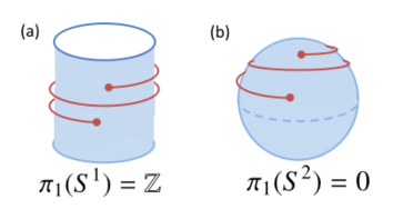
Figure 1: Illustration of topological stability. The stability of a supercurrent is analogous to topological stability of a string wrapped around a surface. (a) The winding number of a string wrapped around a rod is topologically stable and it can not be unravelled (b) A string wrapped around the equator of a sphere unravels due to a lack of topological stability.

General arguments tell us that the condition for the stability of a superfluid is determined by the order parameter manifold or “coset space” $G/H$ formed between the symmetry group $G$ of the Hamiltonian and the invariant subgroup $H$ of the order parameter. The absence of coherent bulk superflow requires that the first homotopy class $\pi_{1}(G/H)\neq{\mathbb{Z}}$ is sparse, lacking the infinite set of integers which protect macroscopic winding of the phase. This means that $G/H$ is a higher dimensional non-Abelian coset space, most naturally formed through the condensation of bosons or Cooper pairs with angular momentum. Thus in spinor Bose gases, an atomic spinor condensate lives on an $SU(2)$ manifold with $\pi_{1}(SU(2))=0$: in this case the observed decay of vorticity gives rise to Rabi oscillationsMatthews et al. (1999). Similarly, in superfluid ³He-A, an $SO(3)$ manifold associated with a dipole-locked triplet paired stateVollhardt and Wölfle (1990); Volovik (2003), for which $\pi_{1}(SO(3))=Z_{2}$ allows a single vortex, but no macroscopic circulation in the bulk

In the solid state, the conditions for a topological failure of superconductivity are complicated by crystal anisotropy. On the one hand, if the condensate carries orbital angular momentum, it will tend to lock to the lattice, collapsing the manifold back to $U(1)$. On the other hand, if the order parameter has s-wave symmetry, its $U(1)$ coset space allows stable vortices.

There are however two ways around this no-go argument. The first, is if there is an additional “isospin” symmetry of the order parameter. For example, the half-filled attractive Hubbard modelMoreo and Scalapino (1991), which forms a “supersolid” ground-state with a perfect spherical ($S^{2}$) manifold of degenerate charge density and superconducting states, with pure superconductivity along the equator and a pure density wave at the pole. In this special case, supercurrents can always decay into a density wave.

A second route is suggested by crystal field theory, which allows the restoration of crystalline isotropy for low spin objects, such as a spin 1/2 ferromagnet in a cubic crystal. Were an analogous s-wave spin-triplet condensate to form, isotropy would be assured. Rather general arguments suggest that the way to achieve an s-wave spin triplet, is through the development of odd-frequency pairing. The Gorkov function of a triplet condensate has the form

$${\bf d}(1-2)=\langle\psi_{\alpha}(1)(i\sigma_{2}\vec{\sigma})_{\alpha\beta}\psi_{\beta}(2)\rangle.$$ (1)

where $1\equiv(\vec{x}_{1},t_{1})$ and $2\equiv(\vec{x}_{2},t_{2})$ are the space-time co-ordinates of the electrons. Exchange statistics enforce the pair wavefunction ${\bf d}(X)=-{\bf d}(-X)$ to be odd under particle exchange. Conventionally, ${\bf d}(\vec{x},t)=-{\bf d}(-\vec{x},t)$ is an odd function of position, leading to odd-angular momentum pairs. By contrast, an s-wave triplet is even in space and must therefore be odd in time, ${\bf d}(|x|,t)=-{\bf d}(|x|,-t)$, as first proposed by Berezinsky Berezinskii (1974); Balatsky and Abrahams (1992); Coleman et al. (1994); Abrahams et al. (1995); Bergeret et al. (2005); Eschrig (2015). Odd-frequency triplet pairing has been experimentally-established as a proximity effect in hybrid superconductor-ferromagnetic tunnel junctionsBergeret et al. (2005); Eschrig (2015). But for spontaneous odd-frequency pairing, we need to identify an equal-time order parameter. Following Abrahams et al. (1995), we can do this by writing the time derivative of the Gorkov function using the Heisenberg equation of motion:

$${\mathbf{\Psi}}(1)=\left.\frac{\partial{\bf d}(1-2)}{\partial t_{1}}\right|_{1=2}=\langle[\psi_{\alpha}(1),H](\sigma_{2}\vec{\sigma})_{\alpha\beta}\psi_{\beta}(1)\rangle.$$ (2)

The specific form of this composite operator depends on the microscopic physics, but the important point to notice is that it is an equal-time expectation value which defines a complex vector order parameter ${\mathbf{\Psi}}={\mathbf{\Psi}}_{1}+i{\mathbf{\Psi}}_{2}$.

The case of SmB₆ motivates us to examine a concrete example of this idea. We consider a Kondo lattice of local moments (${\bf S}_{j}$) interacting with electrons via an exchange interaction of form $H=J\sum_{j}{\bf S}_{j}\cdot\psi^{\dagger}(x_{j})\vec{\sigma}\psi(x_{j})$. In this case, the crucial commutator has the form $[\psi_{\alpha}(x),H]=J({\bf S}(x)\cdot\vec{\sigma})_{\alpha\gamma}\psi_{\gamma}(x)$, giving rise to an equal-time, composite pair order parameter between local moments and s-wave pairs Emery and Kivelson (1992); Abrahams et al. (1995)

$${\mathbf{\Psi}}(x)\propto\langle\psi_{\uparrow}(x)\psi_{\downarrow}(x){\bf S}(x)\rangle.$$ (3)

In microscopic theory, it is actually more natural to consider an antiferromagnetic version of composite order, formed between the staggered magnetization and the pair density, ${\mathbf{\Psi}}(x)=(-1)^{i+j+k}\langle\psi_{\uparrow}(x)\psi_{\downarrow}(x){\bf S}(x)\rangle$ Emery and Kivelson (1992); Coleman et al. (1994); Zachar and Tsvelik (2001); Berg et al. (2010). These details do not however affect the development of the phenomenology.

We now consider a general Ginzburg Landau free energy for an s-wave triplet condensate. Unlike a p-wave triplet, the absence of orbital components to the order parameter considerably simpifies the Ginzburg Landau free energy densityKnigavko et al. (1999),

$$f=\frac{1}{2m}|(-i\hbar\nabla-2e\vec{A}){\mathbf{\Psi}}|^{2}+a|{\mathbf{\Psi}}|^{2}+b|{\mathbf{\Psi}}^{*}\cdot{\mathbf{\Psi}}|^{2}+d|{\mathbf{\Psi}}\cdot{\mathbf{\Psi}}|^{2},$$ (4)

where $\vec{A}$ is the vector potential, minimally coupled to the order parameter. Provided $d>0$, the condensate energy is minimized when ${\mathbf{\Psi}}\cdot{\mathbf{\Psi}}=0$ and the real and imaginary parts of the order parameter are orthogonal ${\bf\Psi}=|\Psi|(\hat{\rm{\bf l}}+i\hat{\bf m})$. The triplet odd-frequency order parameter thus defines a triad $(\hat{\bf l},\hat{\bf m},\hat{\bf n})$ of orthogonal vectors with principal axis $\hat{\bf n}=\hat{\bf l}\times\hat{\bf m}$.

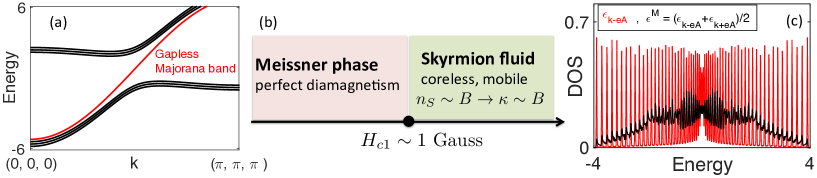
Figure 2: (a) Hybridization of 3 localized Majorana fermions per spin with 4 Majorana fermions of the conduction band leads to one gapless Majorana Fermi surface. (b) Magnetic field phase diagram of a Skyrme insulator. (c) Landau quantization of the projected Majorana Fermi surface.

Eliminating the amplitude degrees of freedom (see supplementary material)Coleman et al. (1994); Knigavko et al. (1999), the long-wavelength action has the following form

$${\cal F}=\int d^{4}x\left[\frac{\rho_{\perp}}{2}(\partial_{\mu}\hat{\bf n})^{2}+\frac{\rho_{s}}{2}(\omega_{\mu}-qA_{\mu})^{2}+\frac{F_{\mu\nu}^{2}}{16\pi}\right].$$ (5)

Here $q=2e/\hbar$, and we have adopted the relativistic limit of the action to succinctly include both electric and magnetic fieldsfoo , using the Minkowski signature ($x_{\mu}^{2}\equiv\vec{x}^{2}-x_{0}^{2}$ with $c=1$) and denoting $A_{\mu}=(-V,\vec{A})$ as the four-component vector potential. The first two terms describe the condensate action, where $\omega_{\mu}=\hat{\bf m}\cdot\partial_{\mu}\hat{\bf l}$ is the rate of precession of the order parameter about the $\hat{\bf n}$ axis. $\rho_{s}$ is the nominal superfluid stiffness, while $\rho_{\perp}$ determines the magnetic rigidity. The last term is the field energy, where $F_{\mu\nu}=\partial_{\mu}A_{\nu}-\partial_{\nu}A_{\mu}$ is the electromagnetic field tensor. The stiffness coefficients $\rho_{\perp},\rho_{s}$ are temperature dependent and are obtained by integrating out the thermal and quantum fluctuations of the microscopic degrees of freedom. Under the gauge transformation $(\hat{\bf l}+i\hat{\bf m})\rightarrow e^{i\phi}(\hat{\bf l}+i\hat{\bf m})$ and $qA_{\mu}\rightarrow qA_{\mu}+\partial_{\mu}\phi$, the vectors $\hat{\bf l}$ and $\hat{\bf m}$ rotate through an angle $\phi$ about the $\hat{\bf n}$ axis, so the angular gradient transforms as $\omega_{\mu}\rightarrow\omega_{\mu}+\partial_{\mu}\phi$, and thus the currents ${J}^{\mu}=q\rho_{s}(\omega^{\mu}-q{A}^{\mu})$ and free energy are gauge invariant. The equivalence of electron gauge transformations and spin-rotation means that gauge transformations are entirely contained within the $SO(3)$ manifold of the order parameter.

To analyze how the superflow is destablized, we examine the screening of electromagnetic fields. From Ampères equation $4\pi J^{\mu}=\partial_{\nu}F^{\mu\nu}$, we observe if $\partial_{\nu}F^{\mu\nu}=0$, corresponding to uniform internal fields, then the supercurrent vanishes ${J}^{\mu}=q\rho_{s}(\omega^{\mu}-q{A}^{\mu})=0$. In a superconductor, this condition is only be achieved by the complete exclusion of fields, but here the texture of the composite order parameter is able to continually adjust with the vector potential so that $\omega^{\mu}=qA^{\mu}$, enabling the current to vanish in the presence of internal fields. To examine this further, we take the curl of Ampères equation, to obtain

$$(1-\lambda_{L}^{2}\partial^{2})F^{\mu\nu}=q^{-1}\Omega^{\mu\nu},$$ (6)

where $\lambda_{L}=(4\pi q^{2}\rho_{s})^{-1/2}$ is the London penetration depth. This modified London equation contains the additional term $\Omega^{\mu\nu}=\partial^{\mu}\omega^{\nu}-\partial^{\nu}\omega^{\mu}$, which is the curl of the gradient of the order parameter. In a conventional superconductor, $\omega^{\mu}=\partial^{\mu}\phi$ is the gradient of the superconducting phase so $\Omega^{\mu\nu}=0$ vanishes causing fields to be expelled. However in a Skyrme insulator, the quantity $\Omega^{\mu\nu}$ is finite, and can be written in the form ${\Omega^{\mu\nu}}={\hat{\bf n}}\cdot(\partial^{\nu}{\hat{\bf n}}\times\partial^{\mu}{\hat{\bf n}})$, which is a the Mermin-Ho relationSM for the skyrmion density of the $\hat{\bf n}$ field. From (6), we see that on scales long compared with the penetration depth, where gradients of the field can be neglected, the average skyrmion density locks to the average external field, $\overline{\Omega^{\mu\nu}}=q\overline{F^{\mu\nu}}$, where the lines denote a coarse-grained average. This relation expresses the screening of supercurrents by the skyrmions, and it also holds in non-relativistic versions of this theoryfoo . Moreover, phase rotations around the $\hat{\bf n}$ axis are now absorbed into the electromagnetic field (Anderson Higg’s effect), leaving behind a residual order parameter manifold with $SO(3)/U(1)\equiv S^{2}$ symmetry. While the homotopy analysis yields no stable vortices $\pi_{1}(S^{2})=0$, it does allow for the topologically stable skyrmion solutions $\pi_{2}(S^{2})=\mathbb{Z}$ that screen the superflow and allow penetration of electric and magnetic fields. We shall actually consider lines of skyrmion , formed by stacking two dimensional skyrmion configurations, similar to vortex lines in three dimensional superconductors. We call the corresponding dielectric a “Skyrme insulator”.

Written in non-relativistic language, the equations relating the skyrmion density to the penetrating fields are

$$\frac{1}{2\pi}\overline{{\hat{\bf n}}\cdot(\partial_{i}{\hat{\bf n}}\times\partial_{j}{\hat{\bf n}})} = -\epsilon_{ijk}\left(\frac{B_{k}}{\Phi_{0}}\right)$$ (7)

$$\frac{1}{2\pi}\overline{{\hat{\bf n}}\cdot(\partial_{i}{\hat{\bf n}}\times\partial_{t}{\hat{\bf n}})} = \frac{2e}{h}{E_{i}}$$ (8)

where $\Phi_{0}=2\pi/q=h/2e$ is the flux quantum, and the overline denotes a coarse-grained average over space or time. The first term in (34) relates the areal density of skyrmions to the magnetic field, allowing a magnetic field to penetrate with a density of one flux quantum per half-skyrmion or “meron”. The second term in (34) describes the unravelling of supercurrents due to phase slippageAnderson and Toulouse (1977) created by domain wall or instanton configurations of the order parameter. The integral of this term over a time $t$ and length $L$ of the wire, counts the number of domain-walls $N=-\frac{2e}{h}(V_{2}-V_{1})t$ crossing the wire in time $t$, in the presence of a finite voltage drop $V_{2}-V_{1}$. This voltage generation mechanism is similar to the development of insulating behavior in disordered two-dimensional superconductorsFisher et al. (1990). We conclude that the failure of the superconductivity does not reinstate a metal, which would screen out electric fields, but instead transforms it into a dielectric into which both electric and magnetic fields freely penetrate.

Unlike vortices, skyrmions are coreless, with short-range interactions, so we expect them to form an unpinned liquid, analogous to the vortex liquid of type II superconductors, which restores the broken $U(1)$ symmetry on macroscopic scales. How then would we distinguish a Skyrme insulator from a more conventional dielectric? Since the density of merons (half skyrmions) $n_{s}=B/\Phi_{0}$ is proportional to a magnetic field, one signature of a skyrmion liquid is a thermal conductivity $\kappa\propto H$ proportional to the applied field $H$. In a Drude model, the drift velocity $v_{d}=\mu(-\nabla T)$ is proportional to the temperature gradient and the skyrmion mobility $\mu$. If ${\cal Q}$ is the heat content per unit length, then $\kappa={\cal Q}\mu n_{S}$, so that

$$\kappa=\left(\frac{\mu{\cal Q}}{\Phi_{0}}\right)H.$$ (9)

is proportional to the applied field.

A further consequence is the development of a low field Meissner phase. In a fixed external magnetic field ${\bf H}$, we consider the Gibb’s free energy ${\cal G}={\cal F}-\int d^{3}x{\bf H}\cdot{\bf B}(x)/(4\pi)$. Taking the field to lie in the z-direction and re-writing the field $B_{z}=n_{S}(x)\Phi_{0}$, where $n_{S}=\frac{1}{2\pi}\Omega^{12}$ is the areal meron density, then

$${\cal G}=\int d^{3}x\left[\frac{\rho_{\perp}}{2}(\partial_{\mu}{\bf n})^{2}+\frac{(H-\Phi_{0}{n_{S}}(x))^{2}}{8\pi}-\frac{H^{2}}{8\pi}\right],$$ (10)

This corresponds to an $O(3)$ sigma model in which the skyrmions have a finite chemical potential $\mu_{S}=\Phi_{0}H/4\pi$, per unit length. Suppose the corresponding energy of a skyrmion is $\epsilon_{S}/a$ per unit length, where $a$ is the lattice spacing, then providing $H<H_{c}=4\pi\epsilon_{S}/\Phi_{0}a$, the skyrmion energy will exceed the chemical potential, and they will be excluded from the fluid. Reverting to SI notation, this becomes

$$\mu_{0}H_{c}=\frac{4}{137}\left(\frac{V_{S}}{ac}\right),$$ (11)

where we have replaced $\frac{e^{2}}{\hbar c}=1/137$, the fine structure constant and $\epsilon_{S}=eV_{S}$. Below this field, skyrmions and field lines will be expelled, so the material will exhibit a Meissner effect. A generic phase diagram is given in Fig. 2(b).

We now discuss the possible microscopic origin of this kind of order, and its possible application to SmB₆. Various anomalous aspects of insulating SmB₆ can be speculatively associated with the properties of a Skyrme insulator. The recent observation of an unusual thermal conductivity in insulating SmB₆, that is linear in field, $\kappa\propto H$Sebastian (2016) is most naturally interpreted as a kind of flux liquid expected in such a phase, a hypothesis that could be checked by confirming that this anomalous thermal conductivity is only exhibited perpendicular to the field direction.

A second test of this hypothesis, is the magnetic susceptibility. In a heavy fermion compound, the order parameter stiffness $\rho$ is set by the Kondo temperature $T_{K}$, $\rho\sim k_{B}T_{K}/a$Coleman et al. (1994), where $a$ is the lattice spacing, so the the energy of a skyrmion is approximately $k_{B}T_{K}$ per unit lattice spacing $a$ and $eV_{K}\sim k_{B}T_{K}$. For SmB₆ we estimate $V_{K}=1meV$, and with $a=10^{-9}m$ we obtain $\mu_{0}H_{c}\sim 10^{-4}T$ or 1 Gauss, comparable with the earth’s magnetic field. In a magnetically screened ($\mu-$ metal) environment we expect SmB₆ to become fully diamagnetic with magnetic susceptibililty $\chi=-1/4\pi$.

A microscopic model for the development of composite order in a Kondo lattice was studied by Coleman, Miranda and TsvelikColeman et al. (1994, 1993) (CMT) and recently revisited by BaskaranBaskaran (2015). This model allows us to pursue the consequences of the failed-superconductivity hypothesis into the microscopic domain. In a conventional Kondo lattice the local moments fractionalize into charged Dirac fermions; the CMT model considers an alternative fractionalization of the local moments into Majorana fermions. In the corresponding mean-field theory, spin $1/2$ local moments $\bf S$ are represented as a bilinear of ${\bf S}=-\frac{i}{2}\bm{\hat{\eta}}\times\bm{\eta}$, where $\bm{\hat{\eta}}=(\hat{\eta}_{x},\hat{\eta}_{y},\hat{\eta}_{z})$ is a triplet of Majorana fermions. In this representation, the Kondo interaction factorizes as follows:

$$H_{K}[i] = J_{K}(\hat{\psi}_{i\alpha}^{\dagger}\bm{\sigma}_{\alpha\beta}\hat{\psi}_{i\beta})\cdot{\bf S}_{i}$$ (12)

$$\rightarrow \biggl{[}\hat{\psi}_{i\alpha}^{\dagger}(\bm{\sigma}_{\alpha\beta}\cdot\hat{\bm{\eta}}_{i}){\cal V}_{i\beta}+{\rm H.c}\biggr{]}+{{\cal V}_{i}^{\dagger}{\cal V}_{i}}/J_{K},$$

where $J_{K}$ is the Kondo interaction strength, $c^{\dagger}_{i\gamma}$ creates a conduction electron and $[{\cal V}_{i}]_{\beta}=-\frac{J_{K}}{2}\langle(\bm{\sigma}_{\beta\gamma}\cdot\bm{\eta}_{i})c_{i\gamma}\rangle$ is a two-component spinor. ${\cal V}_{j}$ determines the composite order via the equation $\vec{\Psi}({\bf x})={\cal V}^{T}i\sigma_{2}\vec{\sigma}{\cal V}$. We have extended the CMT model to include spin-orbit coupling by incorporating a ‘p-wave’ form factor into the definition of the conduction Wannier states $c_{i}$, derived from the angular momentum difference $|\Delta l|=1$ between the heavy $f$ and light $d$ electronsSM ; Alexandrov et al. (2015). Our mean-field calculations confirm that even in the presence of the spin-orbit coupling, the ground-state energy is independent of the orientation of the composite order parameter $\vec{\Psi}$, so the system remains isotropicSM .

In the CMT model, the conduction electrons, represented by four degenerate Majorana bands, hybridize with the three neutral Majorana fermions, gapping all but one of them which is left behind to form a gapless Majorana Fermi sea [Fig 2 (a)]. This unique feature provides an appealing explanation of the robust linear specific heat $C_{v}=\gamma T$ observed in this material. The neutrality of the Majorana Fermi sea eliminates the strictly DC conductivity, but the current and spin matrix elements are actually proportional to energy, which will lead to a quasiparticle optical conductivity of the form

$${\rm Re}[\sigma(\omega)]=\frac{\sigma_{0}}{1+\omega^{2}\tau^{2}}\omega^{2},$$ (13)

where $\tau$ is the relaxation rate. The analogous matrix element effect also suppresses the Koringa spin relaxation rate, giving rise to a $T^{3}$ NMR relaxation rateColeman et al. (1993). When we include the spin-orbit coupling, we find that an additional topological Majorana surface state develops, reminiscent of the Majorana surface states of superluid He-3. This interesting state is protected by the crystal mirror symmetry and decouples from the gapless bulk band. Thus the insulating state retains some of the surface conductivity of a topological Kondo insulatorDzero et al. (2010); Wolgast et al. (2013).

Perhaps the most puzzling aspect of SmB₆ is the reported observation of 3D bulk quantum oscillations. An approximate treatment of the effect of a magnetic field on the Majorana Fermi surface can be made by initially ignoring the skyrmion fluid background. The dispersion of the Majorana band in a field can then be calculated by projecting the Hamiltonian into the low-lying Majorana band.

$$\epsilon^{\rm M}_{\bf k,A}=\langle\phi^{\rm M}_{\bf k}|H({\bf k,A})|\phi^{\rm M}_{\bf k}\rangle=\frac{1}{2}(\epsilon^{\rm e}_{{\bf k}-e{\bf A}}+\epsilon^{\rm h}_{{\bf k}+e{\bf A}}),$$ (14)

where $\epsilon^{\rm e}_{\bf k-eA}$ and $\epsilon^{\rm h}_{\bf k+eA}$ are the dispersion for electrons and holes which couple to the external gauge field with opposite signs. Although the scattering off the triplet condensate mixes the electron and hole components of the field, giving rise to a neutral quasiparticles for which current operator $J_{\alpha}=\partial\epsilon^{\rm M}_{\bf k,A}/\partial A_{\alpha}|_{\bf A=0}=0$ vanishes, this cancellation does not extend to the second derivative of the energy $\partial^{2}\epsilon^{\rm M}_{\bf k,A}/\partial{A_{\alpha}}^{2}|_{\bf A=0}\neq 0$ which is responsible for the diamagnetic response. This is a consequence of the broken gauge-invariant environment provided by the Skyrme insulator. In Fig. 2(c), we show the density of states of the Majorana band in a magnetic field, demonstrating a discrete Landau quantization with broadened Landau levels. Since quantum oscillations originate from the discretization of the density of states into Landau levels, we anticipate that a Majorana Fermi surface does give rise to quantum oscillations. Moreover since the Majorana Fermi surface originates predominantly from the conduction electron band, it has a small effective mass, in accordance with quantum oscillation experimentsLi et al. (2014); Tan et al. (2015).

We note that triplet odd frequency pairing is expected to be highly prone to disorder. Weakly disordered samples may indeed revert to a topological Kondo insulating phase, at least in the majority of the sample. This may account for the marked sample dependence, and the discrepancies between samples grown by different crystal growth techniques. Nevertheless, we expect that small patches of failed superconductivity will still lead to enhanced diamagnetism in a screened ($\mu-$ metal) environment.

Our results also set the stage for a broader consideration of failed superconductivity in other strongly correlated materials. There are several known Kondo insulators with marked linear specific heat coefficients, including Ce₃Bi₄Pt₃Jaime et al. (2000), CeRu₄Sn₆Brüning et al. (2010) and CeOs₄As₁₂Baumbach et al. (2008) which might fall into this class. We end by noting that Skyrme insulators may also be relevant in an astrophysical context such as color superconductivity in white dwarf or neutron starsGinzburg (1969); Alford et al. (2008).

We thank Peter Armitage, Eric Bauer, Michael Gershenson, Andrew Mackenzie, Filip Ronning and Suchitra Sebastian for useful discussions related to this work. This work was supported by the Rutgers Center for Materials Theory group postdoc grant (Po-Yao Chang), Piers Coleman and Onur Erten were supported by the U.S. Department of Energy basic energy sciences grant DE-FG02-99ER45790. Piers Coleman and Onur Erten also acknowledge the hospitality of the Aspen Center for Physics, which is supported by National Science Foundation grant PHY-1066293. Alexei Tsvelik was supported by the U.S. Department of Energy (DOE), Division of Condensed Matter Physics and Materials Science, under Contract No. DE-AC02-98CH10886.

Supplementary Material for “Skyrme insulators: insulators at the brink of superconductivity. ”

These supplementary materials describe the details behind the phenomenology of a Skyrme insulator, and the underlying microscopic mean-field theory.

I Phenomenology

I.1 Ginzburg-Landau theory

To illustrate the idea of a Skyrme insulator, we consider a superconductor with a complex vector order parameter $\vec{\Psi}$. In our microscopic realization of this phenomenon, the complex vector order parameter is a consequence of underlying odd-frequency triplet pairing, which gives rise to composite order between the pair density of a conduction sea, and the staggered magnetization of a Kondo lattice, given by

$$\vec{\Psi}({\bf x})=\left(-1\right)^{i+j+k}\langle\psi_{\uparrow}\psi_{\downarrow}{\bf S}({\bf x})\rangle={\frac{|\vec{\Psi}({\bf x})|}{\sqrt{2}}}\biggl{(}\hat{\rm{\bf l}}({\bf x})+i\hat{\bf m}({\bf x})\biggr{)},$$ (1)

where $\psi_{\uparrow}\psi_{\downarrow}$ is the pair density and $\left(-1\right)^{i+j+k}{\bf S}({\bf x})$ is the staggered magnetization.

However, the long-wavelength action can be developed independently of the microscopic theory by considering the Landau Ginzburg theory of a complex vector $\vec{\Psi}$. The first part of our derivation closely follows referenceKnigavko et al. (1999). Considering terms up to quartic order, the most general isotropic Landau Ginzburg free energy functional of a complex three component vector $\vec{\Psi}$ is given by

$${\cal F}[\Psi]=\int d^{3}xf[\Psi],$$ (2)

where

$$f[\Psi] = \frac{\hbar^{2}}{2m}|(\partial_{j}+iq{A}_{j})\vec{\Psi}|^{2}+a|\vec{\psi}|^{2}$$ (3)

$$+ b|\vec{\Psi}^{*}\cdot\vec{\Psi}|^{2}+d|\vec{\Psi}\cdot\vec{\Psi}|^{2}+e|\vec{\Psi}\times\vec{\Psi}^{*}|^{2},$$ (4)

where $q=2e/(\hbar c)$ and summation over $j\in[1,3]$ is implied. By re-writing $|\vec{\Psi}\times\vec{\Psi}^{*}|^{2}=|\vec{\Psi}|^{4}-|\vec{\Psi}\cdot\vec{\Psi}|^{2}$, and changing $b\rightarrow b-e$, $d\rightarrow d+e$, we can absorb the last quartic term into redefinitions of $b$ and $d$, so that

$$f[\Psi]=\frac{\hbar^{2}}{2m}|(\partial_{j}+iq{A}_{j})\vec{\Psi}|^{2}+a|\vec{\Psi}|^{2}+b|\vec{\Psi}^{*}\cdot\vec{\Psi}|^{2}+d|\vec{\Psi}\cdot\vec{\Psi}|^{2}$$ (5)

Splitting the order into its real and imaginary components, $\vec{\Psi}=\vec{\Psi}_{1}+i{\vec{\Psi}}_{2}$, then

$$|\vec{\Psi}\cdot\vec{\Psi}|^{2}=(|\Psi_{1}|^{2}-|\Psi_{2}|^{2})^{2}+4|\vec{\Psi}_{1}\cdot\vec{\Psi}_{2}|^{2}.$$ (6)

If $d>0$, it follows that the energy is minimized by configurations in which $\vec{\Psi}_{1}$ and $\vec{\Psi}_{2}$ are orthogonal, and of equal magnitude $|\Psi|$, so that $\vec{\Psi}\cdot\vec{\Psi}=0$. It follows that the order parameter has the general form

$$\vec{\Psi}(x)={\frac{|\Psi(x)|}{\sqrt{2}}}(\hat{\bf l}(x)+i\bf{\hat{m}}(x)).$$ (7)

(Note that the equivalent form ${\frac{|\Psi(x)|}{\sqrt{2}}}(\hat{\bf l}(x)-i\bf{\hat{m}}(x))$ can be transformed into the above by a 180⁰ rotation in spin space about the $\hat{\bf l}$ axis.) In these new variables the amplitude variables separate out from the orientational degrees of freedom, and the Landau Ginzburg free energy takes the following form

$$f[\Psi] = \frac{\hbar^{2}}{2m}|(\partial_{j}|\Psi|)^{2}+a|\Psi|^{2}+b|\Psi|^{4}$$ (8)

$$+ \frac{\hbar^{2}}{2m}{\frac{|\Psi|^{2}}{2}}(\partial_{j}+iq{A}_{j})(\hat{\bf l}+i\bf{\hat{m}})|^{2}$$ (9)

Now if $\hat{\bf n}=\hat{\bf l}\times\bf{\hat{m}}$, then $(\hat{\bf l},\hat{\bf m},\hat{\bf n})$ forms a right-handed basis. We can re-write the derivatives of the basis vectors in terms of an angular velocity $\hat{\mathbf{\omega}}$, such that $\partial_{j}(\hat{\bf l},\hat{\bf m},\hat{\bf n})=\hat{\mathbf{\omega}}_{j}\times(\hat{\bf l},\hat{\bf m},\hat{\bf n})$. It follows that:

$$\partial_{j}(\hat{\bf l}+i\hat{\bf m}) = {\hat{\mathbf{\omega}}_{j}}\times(\hat{\bf l}+i\hat{\bf m}),$$ (10)

$$(\partial_{j}+iqA_{j})(\hat{\bf l}+i\hat{\bf m}) = ({\hat{\mathbf{\omega}}_{j}-qA_{j}\hat{\bf n}})\times(\hat{\bf l}+i\hat{\bf m}).$$ (11)

Decomposing $\hat{\mathbf{\omega}}_{j}=\omega_{j}^{1}\hat{\bf l}+\omega_{j}^{2}\hat{\bf m}+\omega_{j}^{3}\hat{\bf n}$, we can then write

$$\partial_{j}(\hat{\bf l}+i\hat{\bf m}) = (\omega^{2}_{j}\hat{\bf m}+\omega^{3}_{j}\hat{\bf n})\times\hat{\bf l}+i(\omega^{2}_{j}\hat{\bf l}+\omega^{3}_{j}\hat{\bf n})\times\hat{\bf m}$$ (12)

$$= -i\omega^{3}_{j}(\hat{\bf l}+i\hat{\bf m})+i(\omega^{1}_{j}+i\omega^{2}_{j})\hat{\bf n}$$ (13)

and hence

$$(\partial_{j}-iqA_{j})(\hat{\bf l}+i\hat{\bf m}) = -i(\omega^{3}_{j}-qA_{j})(\hat{\bf l}+i\hat{\bf m})$$ (14)

$$+ i(\omega^{1}_{j}+i\omega^{2}_{j})\hat{\bf n}$$ (15)

and hence

$$|(\partial_{j}+iq{A}_{j})(\hat{\bf l}+i\hat{\bf m})|^{2} = \biggl{(}(\omega^{1}_{j})^{2}+(\omega^{2}_{j})^{2}\biggr{)}+2(\omega^{3}_{j}-qA_{j})^{2}$$ (16)

$$= (\partial_{j}\hat{\bf n})^{2}+2(\omega^{3}_{j}-qA_{j})^{2}.$$ (17)

Using these results, the Landau Ginzburg free energy can now be written as

$$f[\Psi] = \frac{\hbar^{2}}{2m}|(\partial_{j}|\Psi|)^{2}+a|\Psi|^{2}+b|\Psi|^{4}$$ (18)

$$+ \frac{\rho_{\perp}}{2}(\partial_{j}\hat{\bf n})^{2}+\frac{\rho_{s}}{2}(\omega^{3}_{j}-qA_{j})^{2}.$$ (19)

where the stiffnesses are given by

$$\rho_{s}=2\rho_{\perp}=\frac{\hbar^{2}|\Psi|^{2}}{m}$$ (20)

If we now neglect the amplitude terms, the final Landau free energy takes the form

$${\cal F}=\int d^{3}\left[\frac{\rho_{\perp}}{2}(\partial_{j}\hat{\bf n})^{2}+\frac{\rho_{s}}{2}(\omega^{3}_{j}-qA_{j})^{2}\right].$$ (21)

I.2 Free energy and action

To go from the free energy functional to the to the action, we now add time-dependent quadratic terms into the free energy functional, writing

$${\cal F}= \int d^{3}xdt\frac{1}{2}\biggl{[}\rho_{\perp}(\partial_{i}\hat{\bf n})^{2}-\chi_{\perp}(\partial_{t}\hat{\bf n})^{2}\biggr{]}$$ (22)

$$+\frac{1}{2}\biggl{[}\rho_{s}(\omega^{3}_{i}-qA_{i})^{2}-\chi_{s}(\omega^{3}_{0}-qA_{0})^{2}\biggr{]}$$

Here $A_{\mu}=(A_{0},\vec{A})=(-cV,\vec{A})$ is the four-component vector potential, where $c$ is the speed of light and $V$ is the scalar potential. The quantities $\chi_{\perp}$ and $\chi_{s}$ are the susceptibilities of the order parameter. In the absence of an electromagnetic field, these give rise to Bolguilubov and spin-waves mode with respective velocities $c_{s}=(\rho_{s}/\chi_{s})^{\frac{1}{2}}$ and $c_{\perp}=(\rho_{\perp}/\chi_{\perp})^{\frac{1}{2}}$. If we now include the action of the electromagnetic field, we obtain

$${\cal F} = \int d^{3}xdt\left(\frac{\rho_{\perp}}{2}\biggl{[}(\partial_{i}\hat{\bf n})^{2}-\frac{1}{c_{\perp}^{2}}(\partial_{t}\hat{\bf n})^{2}\biggr{]}\right.$$ (23)

$$+ \left.\frac{\rho_{s}}{2}\biggl{[}(\omega^{3}_{i}-qA_{i})^{2}-\frac{1}{c_{s}^{2}}(\omega^{3}_{0}-qA_{0})^{2}\biggr{]}+\frac{{\bf B}^{2}-{\bf E}^{2}}{8\pi}\right),$$ (24)

where we use cgs units. This is the non-relativistic version of the theory.

For ease of analysis, it is useful to consider the relativistic limit of this action. Departures from relativistic behavior can easily be added back in at a later stage. In the relativistic version of the theory, $c_{s}=c_{\perp}=c$, the speed of light. In this case, we can rescale the time-components, writing $x^{0}=ct$, so that $\frac{1}{c}\partial_{t}\to\partial_{0}$ and $\frac{1}{c}(\omega_{0}-qA_{0})\to(\omega_{0}-qA_{0})$, where now $A_{\mu}\equiv(A_{0},\vec{A})=(-V,\vec{A})$

The long-wave length action then acquires the manifestly relativistic form

$${\cal F}= \int d^{4}x\left[\frac{\rho_{\perp}}{2}(\partial_{\mu}\hat{\bf n})(\partial^{\mu}\hat{\bf n})+\frac{\rho_{s}}{2}(\omega^{3}_{\mu}-qA_{\mu})(\omega^{3\mu}-qA^{\mu})\right]$$ (26)

$$+\frac{(F_{\mu\nu})^{2}}{16\pi},$$

where we have adopted a relativistic notation with Minkowski metric $g_{\mu\nu}=(-1,1,1,1)$ and $F_{\mu\nu}=\partial_{\mu}A_{\nu}-\partial_{\nu}A_{\mu}$ is the electromagnetic tensor, such that $F_{i0}=E_{i}$ and $F_{ij}=\epsilon_{ijk}B_{k}$ determine the electric and magnetic fields respectively.

To determine Maxwell’s equations in the presence of the order parameter, we take variations with respect to $\delta A^{\mu}$,

$$\delta{\cal F}=\int d^{3}xdt\left[-J_{\mu}+\frac{1}{4\pi}\partial^{\nu}F_{\mu\nu}\right]\delta A^{\mu}$$ (27)

where $J_{\mu}=q\rho_{s}(\omega_{\mu}^{3}-qA_{\mu})$ is the current, so that the Ampéres equation is $\partial^{\nu}F_{\mu\nu}=4\pi J_{\mu}=4\pi q\rho_{s}(\omega_{\mu}^{3}-qA_{\mu})$. In a conventional superconductor $\omega_{\mu}^{3}=\partial_{\mu}\phi$ is just the gradient of a phase, a quantity that can not develop a rotation, and (without vortices) this prohibits solutions in which the magnetic field uniformly penetrates the sample. However, for this SO(3) order parameter, defined by three Euler angles $(\phi,\theta,\psi)$, $\omega_{\mu}^{3}=\partial_{\mu}{\psi}+{\cos\theta}\partial_{\mu}{\phi}$ can develop a non-zero curl. Taking the curl of Ampéres equation we obtain

$$(\partial_{\mu}J_{\nu}-\partial_{\nu}J_{\mu}) = q\rho_{s}(\omega_{\mu\nu}-qF_{\mu\nu})$$ (28)

$$= \frac{1}{4\pi}\left[\partial_{\mu}\partial^{\eta}F_{\nu\eta}-(\mu\leftrightarrow\nu)\right]$$ (29)

$$= \frac{1}{4\pi}\left[\partial_{\mu}\partial^{\eta}(\partial_{\nu}A_{\eta}-\partial_{\eta}A_{\nu})-(\mu\leftrightarrow\nu)\right]$$ (30)

$$= -\frac{1}{4\pi}\partial^{2}F_{\mu\nu}$$ (31)

where $\omega_{\mu\nu}=\partial_{\mu}\omega^{3}_{\nu}-\partial_{\nu}\omega^{3}_{\mu}$ is the curl of the rotation. Rearranging this result gives the London equation

$$\lambda_{L}^{2}\partial^{2}F_{\mu\nu}=F_{\mu\nu}-q^{-1}\omega_{\mu\nu}$$ (32)

where the penetration depth $\lambda_{L}=(4\pi q^{2}\rho_{s})^{-1/2}$. To seek uniform solutions, we set the left-hand side to zero. Using the Mermin-Ho relation, (see Sec. I.4) $\omega_{\mu\nu}=-\hat{\bf n}\cdot(\partial_{\mu}\hat{\bf n}\times\partial_{\nu}\hat{\bf n}),$ when a uniform field penetrates the material, we obtain

$$\frac{\hat{\bf n}\cdot(\partial_{\mu}\hat{\bf n}\times\partial_{\nu}\hat{\bf n})}{2\pi}=-\frac{F_{\mu\nu}}{\Phi_{0}}$$ (33)

where $\Phi_{0}=\frac{2\pi}{q}=\frac{h}{2e}$ is the superconducting flux quantum, in SI units. Identifying $F_{ij}=\epsilon_{ijk}B_{k}$ and $F_{i0}=E_{i}$ this equation can be written as two separate equatins relating the penetrating fields to the skyrmion density,

$$\frac{1}{2\pi}{\hat{\bf n}}\cdot(\partial_{i}{\hat{\bf n}}\times\partial_{j}{\hat{\bf n}}) = -\epsilon_{ijk}\left(\frac{B_{k}}{\Phi_{0}}\right)$$ (34)

$$\frac{1}{2\pi}{\hat{\bf n}}\cdot(\partial_{i}{\hat{\bf n}}\times\partial_{t}{\hat{\bf n}}) = \frac{2e}{h}{E_{i}}.$$ (35)

I.3 Derivation for non-relativistic case

We now repeat the above derivation for the non-relativistic case. If we restore the distinction between $c_{s}$, $c_{\perp}$ and the speed of light, the non-relativistic action is written

$${\cal F} = \int d^{4}x\left(\frac{\rho_{\perp}}{2}\biggl{[}(\partial_{i}\hat{\bf n})^{2}-\frac{c^{2}}{c_{\perp}^{2}}(\partial_{0}\hat{\bf n})^{2}\biggr{]}\right.$$ (36)

$$+ \left.\frac{\rho_{s}}{2}\biggl{[}(\omega^{3}_{i}-qA_{i})^{2}-\frac{c^{2}}{c_{s}^{2}}(\omega^{3}_{0}-qA_{0})^{2}\biggr{]}+\frac{F_{\mu\nu}^{2}}{16\pi}\right),$$ (37)

where $x_{0}\equiv ct$ as in the relativistic case. We see that the modification to the velocities only affects the temporal components of the action. When we take the variation with respect to $A^{\mu}$ the relativistic Ampére equation now contains a correction to the zeroth order term,

$$4\pi q\rho_{s}(\omega_{\mu}^{3}-qA_{\mu})=\partial^{\nu}F_{\mu\nu}+\left(\frac{c_{s}^{2}}{c^{2}}-1\right)\delta_{\mu 0}\partial^{\nu}F_{0\nu}$$ (39)

Taking the curl of this equation and identifying $F_{0i}=-E_{i}$we obtain

$$(F_{\mu\nu}-q^{-1}\omega_{\mu\nu})$$

$$= \lambda_{L}^{2}\left(\partial^{2}F_{\mu\nu}+\left[\frac{c_{s}^{2}}{c^{2}}-1\right](\delta_{\nu 0}\partial_{\mu}-\delta_{\mu 0}\partial_{\nu})\vec{\nabla}\cdot\vec{E}\right).$$ (40)

The magnetic part of this equation, $F_{ij}-q^{-1}\omega_{ij}=\lambda_{L}^{2}\partial^{2}F_{ij}$, ($i,j\in[1,3]$) is unaltered. Identifying $F_{i0}=E_{i}$, the electric part now reads

$$E_{i}-q^{-1}\omega_{i0}=\lambda_{L}^{2}\left[\partial^{2}E_{i}+\left[\frac{c_{s}^{2}}{c^{2}}-1\right]\partial_{i}\vec{\nabla}\cdot\vec{E}\right].$$ (41)

If we decouple the electric field into its longitudinal and transverse components $\vec{E}=\vec{E}^{L}+\vec{E}^{T}$ with $\vec{\nabla}\cdot\vec{E}^{T}=0$ and $\vec{\nabla}\times\vec{E}^{L}=0$ , this becomes

$$E_{i}-q^{-1}\omega_{i0}=\lambda_{L}^{2}\left[\partial^{2}\vec{E}^{T}_{i}+\frac{c^{2}_{s}}{c^{2}}\left({\partial_{i}(\vec{\nabla}\cdot\vec{E}^{L})}-\frac{1}{c_{s}^{2}}\frac{\partial\vec{E}^{L}_{i}}{\partial t^{2}}\right)\right].$$ (42)

The main effect of the non-relativistic equation is to renormalize the velocity $c\rightarrow c_{s}$ and penetration depth $\lambda_{L}\rightarrow\lambda_{T}=(c_{s}/c)\lambda_{L}$ of longitudinal fields. Once again however, the only uniform solutions must satisfy $F_{\mu\nu}=q^{-1}\omega_{\mu\nu}$.

I.4 Mermin-Ho relation

For completeness, here we give the derivation of the Mermin-Ho relation

$$\omega_{\mu\nu}=\partial_{\mu}\omega^{3}_{\nu}-\partial_{\nu}\omega^{3}_{\mu}=-\hat{\bf n}\cdot(\partial_{\mu}\hat{\bf n}\times\partial_{\nu}\hat{\bf n}).$$ (43)

To derive this standard result, we write $\omega^{3}_{\mu}=\hat{\bf m}\cdot\partial_{\mu}\hat{\bf l}$, so that

$$\partial_{\mu}\omega_{\nu}^{3}-\partial_{\nu}\omega_{\mu}^{3}=\partial_{\mu}\hat{\bf m}\cdot\partial_{\nu}\hat{\bf l}-\partial_{\nu}\hat{\bf m}\cdot\partial_{\mu}\hat{\bf l}.$$ (44)

Expanding $\partial_{\mu}(\hat{\bf l},\hat{\bf m})=\hat{\mathbf{\omega}}_{\mu}\times(\hat{\bf l},\hat{\bf m})$, we obtain

$$\partial_{\mu}\omega_{\nu}^{3}-\partial_{\nu}\omega_{\mu}^{3} = (\hat{\mathbf{\omega}}_{\mu}\times\hat{\bf m})\cdot(\hat{\mathbf{\omega}}_{\nu}\times\hat{\bf l})-(\mu\leftrightarrow\nu),$$ (45)

$$= (\omega_{\mu}^{1}\hat{\bf n}-\omega_{\mu}^{3}\hat{\bf l})\cdot(-\omega_{\nu}^{2}\hat{\bf n}+\omega_{\nu}^{3}\hat{\bf m})-(\mu\leftrightarrow\nu),$$ (46)

$$= -(\omega^{1}_{\mu}\omega^{2}_{\nu}-\omega^{1}_{\nu}\omega^{2}_{\mu}).$$ (47)

By contrast,

$$\hat{\bf n}\cdot(\partial_{\mu}\hat{\bf n}\times\partial_{\nu}\hat{\bf n}) = \hat{\bf n}\cdot\left[(\hat{\mathbf{\omega}}_{\mu}\times\hat{\bf n})\times(\hat{\mathbf{\omega}}_{\nu}\times\hat{\bf n})\right],$$ (48)

$$= \hat{\bf n}\cdot\left[(-\omega_{\mu}^{1}\hat{\bf m}+\omega_{\mu}^{2}\hat{\bf l})\times(-\omega_{\nu}^{1}\hat{\bf m}+\omega_{\nu}^{2}\hat{\bf l})\right],$$ (49)

$$= \hat{\bf n}\cdot\left[\omega_{\mu}^{1}\omega_{\nu}^{2}\hat{\bf n}-\omega^{2}_{\mu}\omega_{\nu}^{1}\hat{\bf n}\right],$$ (50)

$$= (\omega_{\mu}^{1}\omega_{\nu}^{2}-\omega_{\nu}^{1}\omega_{\mu}^{2}).$$ (51)

Comparing (45) and (48) gives the Mermin-Ho relation (43).

We can recognize the quantity $\hat{\bf n}\cdot(\delta_{\mu}\hat{\bf n}\times\delta_{\nu}\hat{\bf n})$ as the solid angle subtended by the vector $\hat{\bf n}$ over the rectangle of dimensions $\delta x_{\mu}\times\delta x_{\nu}$. The quantity

$$\frac{\omega_{\mu\nu}}{4\pi}=\frac{\hat{\bf n}\cdot(\partial_{\nu}\hat{\bf n}\times\partial_{\mu}\hat{\bf n})}{4\pi}$$ (52)

thus measures the areal density of skyrmions, where each skyrmion in the order parameter encloses a solid angle $4\pi$. On a taurus

$$\int dxdy\frac{\hat{\bf n}\cdot(\partial_{x}\hat{\bf n}\times\partial_{y}\hat{\bf n})}{4\pi}=N$$ (53)

measures the integer number of skyrmions. The quantity

$$\frac{\omega_{\mu\nu}}{2\pi}=\frac{\hat{\bf n}\cdot(\partial_{\nu}\hat{\bf n}\times\partial_{\mu}\hat{\bf n})}{2\pi}$$ (54)

measures the density of half-skyrmions, or “merons”.

I.5 Effective action in a magnetic field

The purpose of this section is to immerse the Skyrme insulator in an external magnetic field $H$ and to derive the effective long-wavelength action that appears once the internal vector potential has been integrated out of the dynamics. For this calculation, we remove the time-dependent terms in the action, reverting to the free energy. We shall also emply a simplified two dimensional model, introducing the Free energy per layer given by

$$G=a_{0}\int d^{2}x\frac{\rho_{\perp}}{2}(\partial_{\mu}{\bf n})^{2}+\frac{\rho_{s}}{2}(\omega^{3}_{\mu}-qA_{\mu})^{2}$$

$$+\frac{1}{8\pi}[\vec{\nabla}\times{\bf A}]^{2}-\frac{1}{4\pi}{\bf H}\cdot[\vec{\nabla}\times{\bf A}],$$ (55)

where $a_{0}$ is the interlayer distance, ${\bf H}=H\hat{\bf z}$ is a uniform external field in the $z$ direction, such that ${\bf B}(x)={\bf H}+4\pi{\bf M}(x)$ is the microscopic field. The main heuristic result, is that at long distances, the supercurrent term $\omega^{3}_{\mu}-qA_{\mu}\rightarrow 0$, and we can use the relationship (34)

$${\bf B}=\vec{\nabla}\times{\bf A}\rightarrow\Phi_{0}n_{s}(x)$$ (56)

where $\Phi_{0}=2\pi/q=h/2e$ is the flux quantum, and

$$n_{s}(x)=\frac{1}{2\pi}{\hat{\bf n}}\cdot(\partial_{y}\hat{\bf n}\times\partial_{x}\hat{\bf n})$$ (57)

is the meron density (each skyrmion contains two merons), to replace the vector potential terms, so that

$$G=a_{0}\int d^{2}x\left[\frac{\rho_{\perp}}{2}(\partial_{\mu}{\bf n})^{2}+\frac{(H-\Phi_{0}{n_{S}}(x))^{2}}{8\pi}-\frac{H^{2}}{8\pi}\right].$$

We shall actually a more general expression, valid at intermediate distances,

$$G/a_{0} = \int d^{2}x\left[\frac{\rho_{\perp}}{2}(\partial_{\mu}{\bf n})^{2}-\frac{H^{2}}{8\pi}\right]$$ (60)

$$+ \frac{1}{8\pi}\int d^{2}xd^{2}x^{\prime}(H-\Phi_{0}{n_{S}}(\hat{\bf x}))V(|\hat{\bf x}-\hat{\bf x}^{\prime}|)$$

$$\times(H-\Phi_{0}{n_{S}}(\hat{\bf x}^{\prime})),$$

where the Fourier transform of the interaction is given by

$$V({\bf p})=\frac{1}{1+{\bf p}^{2}\lambda_{L}^{2}}$$ (61)

where $\lambda_{L}^{2}=\frac{1}{4\pi\rho_{s}q^{2}}$ and ${\bf p}^{2}=\sum_{i=1,2}p_{i}^{2}$. When the density of vortices is smaller than $4\pi\rho_{s}$ the interaction can be considered as short range and the model becomes an O(3) sigma model with an additional term which induces a skyrmion chemical potential $-H/4\pi$ and a short-range repulsion between skyrmions. The long-wavelength action admits finite energy solutions in which the field penetrates and is compensated by a finite topological charge density.

In the calculation that follows, we set $a_{0}=1$ and $q=1$. Our first step is to gauge away the longitudinal (curl-free) parts of the angular velocity. The rate of rotation around the principle axis of the order parameter $\omega_{\mu}^{3}$ can be decomposed in terms of Euler angles:

$$\omega_{\mu}^{3}=\partial_{\mu}\psi+\cos\theta\partial_{\mu}\phi.$$ (62)

In two dimensions, it can also be separated into a gradient and curl:

$$\omega_{\mu}^{3}=\partial_{\mu}\Psi+\epsilon_{\mu\nu}\partial_{\nu}\eta.$$ (63)

Since the second term is divergence free, this can also be thought of as a decomposition into a longitudinal and transverse component. The curl of the rotation rate

$$\epsilon_{\mu\nu}\partial_{\mu}\omega^{3}_{\nu}=\epsilon_{\mu\nu}\partial_{\mu}\epsilon_{\nu\gamma}\partial_{\gamma}\eta=-\nabla^{2}\eta=2\pi n_{S}\equiv\tilde{n}_{s}$$ (64)

where we have defined $\tilde{n}_{S}\equiv 2\pi n_{S}\equiv\Phi_{0}n_{S}$. Thus the curl of the rotation rate is related to the density of topological charge of the ${\bf n}$ field.

Similarly, we split the vector potential into a longitudinal and transverse component:

$$A_{\mu}=\partial_{\mu}{\Psi}+\epsilon_{\mu\nu}\partial_{\nu}\chi,$$ (65)

where we have choosen a gauge to cancel the longitudinal gauge part of $\omega_{\mu}^{3}$. Then the $A$-dependent term in the free energy becomes

$$(\omega_{\mu}^{3}-A_{\mu})^{2}=[(\epsilon_{\mu\nu}\partial_{\nu}(\chi-\eta)]^{2}=[\partial_{\mu}(\chi-\nu)]^{2}$$ (66)

while

$$\vec{\nabla}\times\vec{A}=-\nabla^{2}\chi.$$ (67)

The Free energy for $H=0$ is

$$G=\int d^{2}x\left(\frac{\rho_{\perp}}{2}(\partial_{\mu}\vec{n})^{2}+\frac{\rho_{s}}{2}[\nabla(\chi-\eta)]^{2}+\frac{1}{8\pi}(\nabla^{2}\chi)^{2}\right).$$

(68)

We can rewrite the coupling between the transverse components of the vector potential and order parameter fields [the last two terms in Eq. (68)], represented by $\chi$ and $\eta$, in momentum space as follows

$$G_{\eta\chi}=\frac{1}{2}\int{\frac{{d^{2}p}}{(2\pi)^{2}}}\left[\rho_{s}{\bf p}^{2}|\chi_{p}-\eta_{p}|^{2}+\frac{1}{4\pi}|{\bf p}^{2}\chi_{p}|^{2}\right],$$ (69)

where $\chi_{p}$ and $\eta_{p}$ are the Fourier components of $\chi$ and $\eta$ in the momentum space, ${\bf p}^{2}=\sum_{i=1,2}p_{i}^{2}$, and $\mathcal{G}_{\eta\chi}$ is the free energy density of the order parameter fields. Minimizing the free energy with respect to $\chi_{p}$ we then get

$$\frac{\delta{\cal G}_{\eta\chi}}{\delta\chi_{p}}=\rho_{s}{\bf p}^{2}(\chi_{p}-\eta_{p})+\frac{1}{4\pi}({\bf p}^{2})^{2}\chi_{p}=0$$ (70)

so that

$$\chi_{p} = \frac{\rho_{s}}{\rho_{s}+{\bf p}^{2}/4\pi}\eta_{p},$$ (71)

$$\eta_{p}-\chi_{p} = \frac{{\bf p}^{2}}{4\pi\rho_{s}+{\bf p}^{2}}\eta_{p}=-\frac{1}{4\pi\rho_{s}+{\bf p}^{2}}\tilde{n}_{S}(p),$$ (72)

and the magnetic field is

$$B^{z}=-\partial_{\mu}^{2}\chi=\frac{\rho_{s}}{\rho_{s}+{\bf p}^{2}/4\pi}\tilde{n}_{S}(p),$$ (73)

so that the total flux is equal to the topological charge of the ${\bf n}$-field.

Substituting (72) into (69), we obtain

$$G_{\eta\chi} = \frac{1}{2}{\int\frac{d^{2}p}{(2\pi)^{2}}}\left[\rho_{s}{\bf p}^{2}\frac{|\tilde{n}_{S}(p)|^{2}}{(4\pi\rho_{s}+{\bf p}^{2})^{2}}+\frac{1}{4\pi}\frac{|\rho_{s}\tilde{n}_{S}(p)|^{2}}{(\rho_{s}+{\bf p}^{2}/4\pi)^{2}}\right]$$ (74)

$$= \frac{1}{8\pi}{\int\frac{d^{2}p}{(2\pi)^{2}}}\frac{\rho_{s}|\tilde{n}_{S}(p)|^{2}}{(\rho_{s}+{\bf p}^{2}/4\pi)^{2}}\left[\frac{{\bf p}^{2}}{4\pi}+\rho_{s}\right]$$ (75)

$$= \frac{1}{8\pi}{\int\frac{d^{2}p}{(2\pi)^{2}}}\frac{|\tilde{n}_{S}(p)|^{2}}{(1+{\bf p}^{2}\lambda_{L}^{2})},$$ (76)

where $\lambda_{L}^{2}=\frac{1}{4\pi\rho_{s}}\equiv\frac{1}{4\pi\rho_{s}q^{2}}$, reinstating $q$. Adding back the gradient term $\frac{\rho_{\perp}}{2}(\partial_{\mu}\hat{\bf n})^{2}$, and converting back to real-space, we obtain

$$G=\int d^{2}x\frac{\rho_{\perp}}{2}(\partial_{\mu}{\bf n})^{2}+\frac{1}{8\pi}\int d^{2}xd^{2}x^{\prime}\tilde{n}_{S}(x)V(|\hat{\bf x}-\hat{\bf x}^{\prime}|)\tilde{n}_{S}(\hat{\bf x}^{\prime}),$$

$$V(p)=\frac{1}{1+{\bf p}^{2}\lambda_{L}^{2}}.$$ (77)

Now if we reinstate the external field $H=H_{z}$, we note that

$$-\int d^{2}x\frac{1}{4\pi}HB(x)$$ (78)

$$= -\frac{1}{4\pi}H\int d^{2}x\int{\frac{d^{2}p}{(2\pi)^{2}}}B(p)e^{i{\bf x}\cdot{\bf p}}$$

$$= -\frac{1}{4\pi}H\int d^{2}x\int{\frac{d^{2}p}{(2\pi)^{2}}}V(p)\tilde{n}_{S}(p)e^{i{\bf x}\cdot{\bf p}}$$ (80)

$$= -\frac{1}{4\pi}H\int d^{2}xd^{2}x^{\prime}d^{2}x^{\prime\prime}V(x^{\prime\prime})\tilde{n}_{S}(x^{\prime})$$

$$\times{{\int\frac{d^{2}p}{(2\pi)^{2}}}}e^{i{\bf p}\cdot({\bf x-x^{\prime}-x^{\prime\prime}})},$$

$$= -\frac{1}{4\pi}H\int d^{2}xd^{2}x^{\prime}V(|x-x^{\prime}|)\tilde{n}_{S}(x^{\prime}),$$ (81)

where the normalization factor of the Fourier transformation is $F(x)=\frac{1}{(2\pi)^{2}}\int d^{2}pF(p)e^{i{\bf p}\cdot{\bf x}}$, $F(p)=\int d^{2}xF(x)e^{-i{\bf p}\cdot{\bf x}}$. We can then incorporate the $-{\bf H}\cdot{\bf B}$ term by writing

$$G= \int d^{2}x\left[\frac{\rho_{\perp}}{2}(\partial_{\mu}{\bf n})^{2}-\frac{H^{2}}{8\pi}\right]$$ (83)

$$+\frac{1}{8\pi}\int d^{2}xd^{2}x^{\prime}\delta\tilde{n}_{S}(\hat{\bf x})V(|\hat{\bf x}-\hat{\bf x}^{\prime}|)\delta\tilde{n}_{S}(\hat{\bf x}^{\prime}),$$

$$V(p)= \frac{1}{1+{\bf p}^{2}\lambda_{L}^{2}}.$$ (84)

where $\delta{\tilde{n}_{S}}(x)=\tilde{n}_{S}(x)-H\equiv\Phi_{0}n_{S}(x)-H$.

II The microscopic Hamiltonian—topological CMT model

The microscopic Hamiltonian is motivated by a Majorana representation of local moments first developed by Coleman, Miranda and Tsvelik (CMT model)Coleman et al. (1994, 1993). In order to incorporate the topological aspects of SmB₆, we consider a ‘p-wave’ Kondo-Heisenberg model.

$$H = \sum_{k,\sigma}(\epsilon_{{\bf k}}-\mu)c_{{\bf k},\sigma}^{\dagger}c_{{\bf k},\sigma}-J_{K}\sum_{j,\alpha,\beta}(\tilde{c}_{j\alpha}^{\dagger}\bm{\sigma}_{\alpha\beta}\tilde{c}_{j\beta})\cdot{\bf S}_{j}$$ (85)

$$-J_{H}\sum_{\langle i,j\rangle}{\bf S}_{i}\cdot{\bf S}_{j},$$

where $c_{{\bf k}\sigma}$ is the electron operator, $\epsilon_{{\bf k}}$ and $\mu$ are the dispersion of conduction electrons and chemical potential, ${\bf S}$ is the Sm⁺³ local moment. $J_{K}$ and $J_{H}$ are the Kondo and Heisenberg exchange. $\tilde{c}_{i\alpha}$ represents the local Wannier orbital which is defined as $\tilde{c}_{i\alpha}=\sum_{j}\Phi_{i,j}^{\alpha,\beta}c_{j\beta}$ in terms of the original conduction electrons. Here, $\Phi^{\alpha,\beta}_{i,j}$ is a ‘p-wave’ form factor, $\Phi_{i,j}^{\alpha,\beta}=-\frac{i}{2}\hat{r}_{ij}\cdot\bm{\sigma}_{\alpha,\beta}$ which results from net angular momentum difference $|\Delta l|=1$ between the heavy $f$ and light $d$ electronsAlexandrov et al. (2015). Next we use a Majorana representation for the spin

$${\bf S}_{j}\to-\frac{i}{2}\bm{\eta}_{j}\times\bm{\eta}_{j}$$ (86)

where $\bm{\eta}_{j}\equiv(\eta^{1}_{j},\eta^{2}_{j},\eta^{3}_{j})$ is a three component vector of Majorana fermions, defined at each site $j$. This representation of the spin ensures that the spin commutation relations and $S^{2}=3/4$ are satisfied. Also note that in this representation the constraint field is automatically fulfilled. Inserting Eq. (86) into Eq. (85)

$$H = \sum_{k,\sigma}(\epsilon_{{\bf k}}-\mu)c_{{\bf k},\sigma}^{\dagger}c_{{\bf k},\sigma}-J_{K}\sum_{\begin{subarray}{c}j,\alpha,\beta\end{subarray}}\tilde{c}_{j\alpha}^{\dagger}\bm{(}\bm{\sigma}_{\alpha\beta}\cdot{\bm{\eta}}_{j})^{2}\tilde{c}_{j\beta}$$ (87)

$$-\frac{J_{H}}{2}\sum_{\langle i,j\rangle}({-i\bm{\eta}_{i}\cdot\bm{\eta}_{j}})^{2}$$

We have used the identity $i\bm{\sigma}\cdot(\bm{\eta}_{j}\times\bm{\eta}_{j})=(\bm{\sigma}\cdot\bm{\eta}_{j})^{2}-3/2$. Next we carry out a mean field decoupling by a Hubbard-Stratonovich transformation on the Kondo interaction:

$$-J_{K}\biggl{[}\tilde{c}^{\dagger}_{j\alpha}(\bm{\sigma}_{\alpha\gamma}\cdot\bm{\eta}_{j})\biggl{]}\biggl{[}(\bm{\sigma}_{\gamma\beta}\cdot\bm{\eta}_{j})\tilde{c}_{j\beta}\biggl{]}$$

$$\to \biggl{[}\tilde{c}_{j\alpha}^{\dagger}(\bm{\sigma}_{\alpha\beta}\cdot{\bm{\eta}_{j}}){V}_{j\beta}+{\rm h.c}\biggr{]}+\frac{{V}_{j\gamma}^{\dagger}{V}_{j\gamma}}{J_{K}},$$ (88)

where the auxiliary field ${V}_{i\beta}$ is a fluctuating variables, integrated within a path integral. In the mean field treatment, we assume ${V}_{j\beta}$ assumes a fixed value at each site. The last term in Eq. (88) is only important in evaluating the mean-field equations, and will be dropped in the discussion that follows.

We also perform a Hubbard-Stratonovich transformation on the spin-fluid,

$$-\frac{J_{H}}{2}\sum_{\langle i,j\rangle}(-i{\bm{\eta}}_{i}\cdot{\bm{\eta}}_{j})^{2}\to\sum_{\langle i,j\rangle}(-i\Delta_{ij}{\bm{\eta}}_{i}\cdot{\bm{\eta}}_{j})+\frac{\Delta_{ij}^{2}}{2J_{H}}$$ (89)

where the field $\Delta_{ij}$ is a real, odd-function of position, $\Delta_{ij}=-\Delta_{ji}=\Delta_{ij}^{*}$. In the simplest mean-field theory, taking the bonds to be uniform, $\Delta_{i,i+\hat{\bf a}}=\Delta$ ($\hat{\bf a}=(\hat{x},\hat{y},\hat{z})$), this term leads to to a momentum-dependent dispersion of Majorana Fermions as follows

$$\sum_{\langle i,j\rangle}-i\Delta_{ij}{\bm{\eta}}_{i}\cdot{\bm{\eta}}_{j}=\sum_{{\bf k}\in\frac{1}{2}BZ}\epsilon_{f}({\bf k}){\bm{\eta}_{\bf k}}^{\dagger}\cdot{\bm{\eta}_{\bf k}},$$ (90)

where $\epsilon({\bf k})=2\Delta(\sin k_{x}+\sin k_{y}+\sin k_{z})$. Here, the momentum sum is restricted over half the Brillouin zone (${\bf k}\in\frac{1}{2}BZ$), because the Fourier transform of real Majorana operators satisfies ${\bm{\eta}}_{-{\bf k}}={\bm{\eta}}^{\dagger}_{{\bf k}}={\frac{1}{\sqrt{N}}\sum_{i}e^{i{\bf k}\cdot{{\bf R}}_{i}}}\bm{\eta}_{i}^{\dagger}$ with $\bm{\eta}_{i}^{\dagger}=\bm{\eta}_{i}$, so that the creation and annihilation operators of the Majorana fields are only independent in half the Brillouin zone. In the following discussion, we will neglect the constant term $\Delta_{ij}^{2}/2J_{H}$.

In the original CMT modelColeman et al. (1994, 1993), a “staggered” order parameter (${\cal V}_{j}=\exp(i{\bf Q}\cdot\hat{\bf R}_{j}/2){\cal V}_{0}$ was found to have the lowest mean-field free energy, where ${\bf Q}=(\pi,\pi,\pi)$ defines a staggered wavevector. In momentum space, this has the effect of transfering a momentum ${\bf Q}/2$ each time a Majorana fermion converts into an electron. The Fourier transformed hybridization term is written

$$H_{hyb}=\sum_{{\bf k}}\left[\tilde{c}^{\dagger}_{{\bf k}}(\bm{\sigma}\cdot\bm{\eta}_{{\bf k}-{\bf Q}/2})V_{0}+V_{0}^{\dagger}(\bm{\sigma}\cdot\bm{\eta}^{\dagger}_{{\bf k}-{\bf Q}/2})\tilde{c}_{{\bf k}}\right]$$

Now by taking the transpose of the second term, we can rewrite the hybridization term in the alternate form

$$H_{hyb} =\sum_{{\bf k}}\left[\tilde{c}^{T}_{{\bf k}}(-i\sigma_{2})({-}\bm{\sigma}\cdot\bm{\eta}^{\dagger}_{{\bf k}-{\bf Q}/2})(i\sigma_{2})V^{*}_{0}+h.c\right] (-\bm{\sigma}^{T}=-i\sigma_{2}\bm{\sigma}i\sigma_{2})$$ (92)

$$=\sum_{{\bf k}}\left[\tilde{c}^{T}_{{\bf k}}(-i\sigma_{2})(\bm{\sigma}\cdot\bm{\eta}_{-{\bf k}+{\bf Q}/2})(i\sigma_{2})V^{*}_{0}+h.c\right] (-\bm{\eta}^{\dagger}_{{\bf k}-{\bf Q}/2}=\bm{\eta}_{-{\bf k}+{\bf Q}/2})$$ (93)

$$=\sum_{{\bf k}}\left[\tilde{c}^{T}_{-{\bf k}}(-i\sigma_{2})(\bm{\sigma}\cdot\bm{\eta}_{{\bf k}+{\bf Q}/2})(i\sigma_{2})V^{*}_{0}+h.c\right] ({\bf k}\rightarrow-{\bf k})$$ (94)

$$=\sum_{{\bf k}}\left[\tilde{c}^{T}_{-{\bf k}+{\bf Q}}(-i\sigma_{2})(\bm{\sigma}\cdot\bm{\eta}_{{\bf k}-{\bf Q}/2})(i\sigma_{2})V^{*}_{0}+h.c\right] ({\bf k}\rightarrow{\bf k}{-}{\bf Q})$$ (95)

$$=\sum_{{\bf k}}\left[{c}^{T}_{-{\bf k}+{\bf Q}}(i\sigma_{2})(\sin k_{l}\ \sigma_{l})(\bm{\sigma}\cdot\bm{\eta}_{{\bf k}-{\bf Q}/2})(i\sigma_{2})V^{*}_{0}+h.c\right] (\tilde{c}^{T}_{{\bf k}}(-i\sigma_{2})=c^{T}_{{\bf k}}(i\sigma_{2})(\sin k_{l}\ \sigma_{l}))$$ (96)

Combining (II) and (92 ), we can write the hybridization in the form

$$H_{hyb} = \frac{1}{2}\sum_{{\bf k}}\chi^{\dagger}_{{\bf k}}\left[(\sin k_{l}\sigma^{l})(\bm{\sigma}\cdot\bm{\eta}_{{\bf k}-{\bf Q}/2}){\cal V}_{0}+h.c\right]$$

$$= \sum_{{\bf k}\in\frac{1}{2}BZ}\chi^{\dagger}_{{\bf k}}\left[(\sin k_{l}\sigma^{l})(\bm{\sigma}\cdot\bm{\eta}_{{\bf k}-{\bf Q}/2}){\cal V}_{0}+h.c\right],$$

where $\sin k_{l}\sigma^{l}\equiv\sin k_{x}\sigma_{x}+\sin k_{y}\sigma_{y}+\sin k_{z}\sigma_{z}$, while

$$\chi_{{\bf k}}=\begin{pmatrix}c_{{\bf k}}\cr-i\sigma_{2}c^{\dagger}_{-{\bf k}+{\bf Q}}\end{pmatrix}$$ (99)

and

$${\cal V}_{0}=\begin{pmatrix}V_{0}\cr i\sigma_{2}V^{*}_{0}\end{pmatrix}.$$ (100)

are four component Balian-Werthammer spinors (the minus sign-distinction is deliberate). Note that the sum over half the Brillouin zone ensures that all creation and annihilation operators in the Hamiltonian are independent.

In this same notation, the conduction electron Hamiltonian is given by

$$H_{c}=\sum_{\bf k}\chi_{\bf k}^{\dagger}\left(\begin{array}[]{cccc}\epsilon_{\bf k}-\mu&0&0&0\\ 0&\epsilon_{\bf k}-\mu&0&0\\ 0&0&-\epsilon_{-{\bf k}+{\bf Q}}+\mu&0\\ 0&0&0&-\epsilon_{-{\bf k}+{\bf Q}}+\mu\end{array}\right)\chi_{\bf k}.$$ (105)

In order to simplify our calculation, we consider the particle-hole symmetric case

$$\epsilon_{{\bf k}} =-\epsilon_{-{\bf k}+{\bf Q}}\equiv\epsilon_{c}(\bf k)$$

$$=-2t_{c}(\cos k_{x}+\cos k_{y}+\cos k_{z})+8t^{\prime}_{c}\cos k_{x}\cos k_{y}\cos k_{z}.$$ (106)

We use Pauli matrices $\bm{\tau}$ as the particle-hole basis in the Balian-Werthamer four-spinor notation. The conduction electron Hamiltonian has a compact form

$$H_{c}=\sum_{\bf k\in\frac{1}{2}BZ}\chi_{\bf k}^{\dagger}(\epsilon_{c}(\bf k)-\mu\tau_{3})\chi_{\bf k}.$$ (107)

Finally, the mean field Hamiltonian can be written as, $H=\sum_{\bf k}\psi_{\bf k}^{\dagger}\mathcal{H}({\bf k})\psi_{\bf k}$ with the single-particle Hamiltonian

$$\mathcal{H}({\bf k})=\left(\begin{array}[]{cc}\epsilon_{c}({\bf k})-\mu\tau_{3}&{\cal V}({\bf k})\\ {\cal V}({\bf k})^{\dagger}&\epsilon_{f}({\bf k})\end{array}\right),$$ (110)

where $\psi_{\bf k}=({c}_{{\bf k}\uparrow},{c}_{{\bf k}\downarrow},-{c}^{\dagger}_{-{\bf k}+{\bf Q}\downarrow},{c}^{\dagger}_{-{\bf k}+{\bf Q}\uparrow},\eta_{{{\bf k}-{\bf Q}/2}}^{x},$ $\eta_{{{\bf k}-{\bf Q}/2}}^{y},\eta_{{{\bf k}-{\bf Q}/2}}^{z})^{\rm T}$ and

$${\cal V}({\bf k})_{\alpha}^{\ \ a}=(s_{k_{l}}\ \sigma^{l})_{\alpha\beta}\sigma^{a}_{\beta\gamma}({\cal V}_{0})_{\gamma}.$$ (111)

where we use summation convention and the short-hand $s_{k_{l}}\equiv\sin k_{l}$. If we choose ${\cal V}_{0}=(V,0,0,V)^{T}$, then the hybridization $V({\bf k})$ takes the form

$${\cal V}({\bf k})=V\left(\begin{array}[]{ccc}s_{k_{x}}-is_{k_{y}}&s_{k_{y}}+is_{k_{x}}&s_{k_{z}}\\ -s_{k_{z}}&-is_{k_{z}}&is_{k_{y}}+s_{k_{x}}\\ -s_{k_{z}}&is_{k_{z}}&-is_{k_{y}}+s_{k_{x}}\\ -s_{k_{x}}-is_{k_{y}}&-s_{k_{y}}+is_{k_{x}}&-s_{k_{z}}\end{array}\right).$$ (116)

II.1 Bulk and surface spectra

The bulk spectrum of the single-particle Hamiltonian has a gapless band shown in Fig. 1(a) . In particular, when $\mu=0$, the gapless quasiparticle lead to a form

$$\phi_{\bf k} = \frac{1}{\sqrt{2(s_{k_{x}}^{2}+s_{k_{y}}^{2}+s_{k_{z}}^{2})}}\Big{[}s_{k_{z}}{c}_{{\bf k}\uparrow}+(s_{k_{x}}-is_{k_{y}}){c}_{{\bf k}\downarrow}$$ (117)

$$+(s_{k_{x}}+is_{k_{y}}){c}^{\dagger}_{-{\bf k+Q}\downarrow}+s_{k_{z}}{c}^{\dagger}_{-{\bf k+Q}\uparrow}\Big{]},$$

where $\phi_{\bf k}=\phi^{\dagger}_{-{\bf k+Q}}$ satisfies the ”twisted Majorana condition”.

In the slab geometry, we observe surface states on $(100)$ and $(010)$ surfaces. The crossings in the $(100)$ surface spectrum are located at $X_{1}=(k_{y},k_{z})=(\pi,0)$ and $X_{2}=(k_{y},k_{z})=(0,\pi)$[see Fig. 1(b)(c)]. We find the surface states are robust under mirror symmetry preserving perturbations.

The stability analysis of the robustness of the surface states is done by adding various symmetry preserving perturbation. Specifically, nonvanishing chemical potential $\mu$ and Zeeman terms on the conduction electrons, $+\mu B_{z}{c}^{\dagger}_{\uparrow}{c}_{\uparrow}$ and $-\mu B_{z}{c}^{\dagger}_{\downarrow}{c}_{\downarrow}$, do not break the mirror symmetry $\mathcal{R}_{z}$. We observe the crossings in the $(100)$ and $(010)$ surface spectra cannot be gapped by adding these mirror symmetry-preserving perturbations. We now analyze the topological origin of the mirror symmetry-protected surface states using an entanglement spectrum and Berry phase analysis.

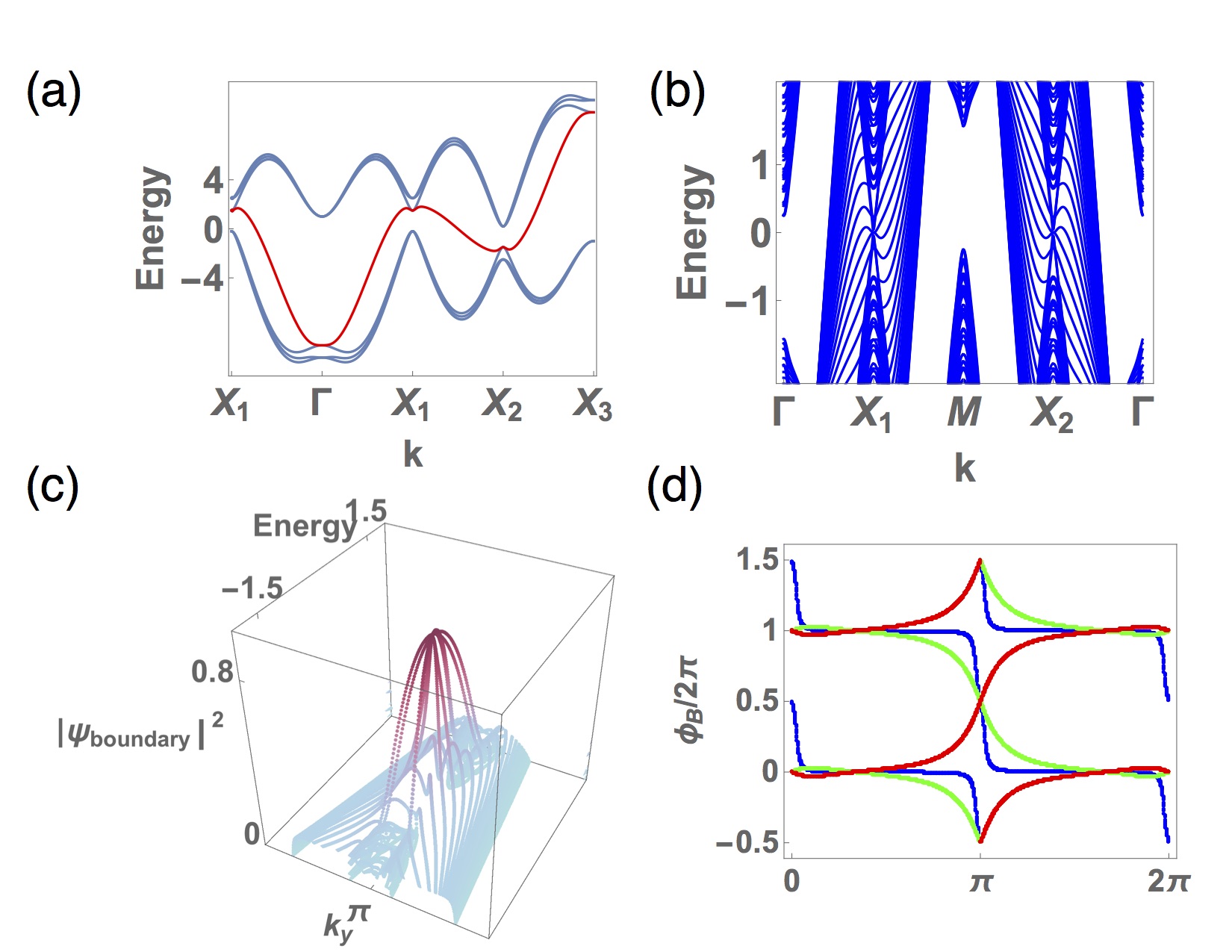
Figure 1: (a) The bulk spectrum with $X_{1}=(\pi,0,0)$, $X_{2}=(\pi,\pi,0)$, and $X_{3}=(\pi,\pi,\pi)$. The red line indicates the gapless Majorana band in the CMT model. (b) The $(100)$ surface spectrum with $X_{1}=(k_{y}=\pi,k_{z}=0)$, $M=(\pi,\pi)$, and $X_{2}=(0,\pi)$. The crossings in the $X_{1}$ and $X_{2}$ are surface states, which the density profile in shown in (c). (c) The density of surface wave function $|\psi_{\rm boundary}|^{2}$ and energy as a function of $k_{y}$ at $k_{z}=0$. The crossings at $k_{y}=0$ are localized states on the $(100)$ surface. (d) The Berry phase as a function of $k_{y}$ at $k_{z}=0$ for the lowest three occupier bands (Blue, Red, Green) with corresponding mirror eigenvalue $(++-)$. The parameters in the CMT model are $(t_{c},t^{\prime}_{c},\alpha,\mu,V)=(1,0.5,0.1,0.5,5)$

II.2 Mirror symmetry protected boundary states and its topological origin

The nonvanishing order parameter $\mathcal{V}$ breaks the time-reversal symmetry and spin-rotation symmetry in the system. The remaining symmetries are the inversion symmetry and the reflection symmetry $\mathcal{R}_{z}$ in the CMT model with $\mathcal{P}^{\dagger}\mathcal{H}({\bf k})\mathcal{P}=\mathcal{H}(-{\bf k})$ and $\mathcal{R}_{z}^{\dagger}\mathcal{H}(k_{x},k_{y},k_{z})\mathcal{R}_{z}=\mathcal{H}(k_{x},k_{y},-k_{z})$, respectively. The matrix representation of the inversion symmetry and reflection symmetry are

$$\mathcal{P}=\left(\begin{array}[]{cc}\tau_{0}\sigma_{0}&0\\ 0&-\mathbb{I}_{3\times 3}\end{array}\right),\quad\mathcal{R}_{z}=\begin{pmatrix}\tau_{3}\sigma_{3}&\cr&R_{z}\end{pmatrix},$$ (120)

where $R_{z}$ is the three dimensional reflection matrix,

$$R_{z}=\begin{pmatrix}1&0&0\\ 0&1&0\\ 0&0&-1\end{pmatrix}.$$ (121)

One should be noticed that the gapless Majorana state is orthogonal to the remaining six gapped states in the energy basis. Thus, the Hilbert space of the CMT model is the direct sum of the two sub-Hilbert spaces, $\mathbb{H}_{\rm CMT}=\mathbb{H}_{\rm gapped}\oplus\mathbb{H}_{\rm gapless}$, where $\mathbb{H}_{\rm gapped/gapless}$ are the sub-Hilbert spaces of the gapped/gapless states respectively. The mirror symmetry protected surface states originate from the gapped bands and we need to extract the information from the gapped sub-Hilbert space $\mathbb{H}_{\rm gapped}$. In order to do this, we perform an entanglement spectrum analysisHughes et al. (2011); Chang et al. (2014) and a Berry phase analysis Taherinejad et al. (2014) for the three lowest occupied bands which belong to $\mathbb{H}_{\rm gapped}$.

In the entanglement spectrum, there are robust mid-gap states protected by inversion symmetry. In Fig. 2(a), the entanglement Hamiltonian is constructed by a bipartition along $z$ direction and the entanglement spectrum is plotted as a function of $k_{y}$ at $k_{x}=\pi$. We observe there are six mid-gap states at $k_{y}=0$ which are protected by inversion symmetry. The topological invariant of inversion symmetric topological phases is given by the number of mid-gap states in the entanglement spectrum, which can be computed from counting the inversion eigenvalues of the occupied bands at inversion symmetric points

$$\nu({\bf k}_{\perp}^{0})=2|N({\bf k}_{\perp}^{0},k_{\parallel}=0)-N({\bf k}_{\perp}^{0},k_{\parallel}=\pi)|,$$ (122)

where ${\bf k}_{\perp}^{0}$ is the inversion symmetric points for the momenta perpendicular to the bipartition direction. $N({\bf k}_{\perp}^{0},k_{\parallel})$ is the number of negative inversion eigenvalue of the occupied band at $k_{\parallel}=0$ or $k_{\parallel}=\pi$, with $k_{\parallel}$ being the momentum along the bipartition directionHughes et al. (2011). For example, if the bipartition is along $z$ direction, $k_{\parallel}=k_{z}$, and ${\bf k}_{\perp}^{0}=(k_{x},k_{y})=(0,0)$, $(0,\pi)$, $(\pi,0)$, and $(\pi,\pi)$.

In the CMT model, the number of mid-gap states is six at both ${\bf k}_{\perp}=(0,\pi)$ and $(\pi,0)$ for the bipartition direction along $x$, $y$ and $z$ directions. Although there is no inversion-symmetry protected surface state in the physical surface spectrum, the mid-gap states in the entanglement spectrum cannot be removed and cannot be adiabatically connected to a system without mid-gap statesHughes et al. (2011); Chang et al. (2014). Thus the CMT model can be seen as an inversion-symmetric topological phase.

On the other hand, we observe physical surface states on $(100)$ and $(010)$ surfaces. These surface states are protected by the reflection symmetry $\mathcal{R}_{z}$. The topological invariant of the mirror-symmetric topological phases is the mirror Chern number at the mirror planes ($k_{z}=0$ and $\pi$). The Chern number is defined as

$$n=\int d{\bf a}\cdot\nabla\times{\bf A}=\oint d{\bf l}\cdot{\bf A},$$ (123)

where $\int d{\bf a}$ is the embedded Brillouin zone of the mirror plane, $\oint d{\bf l}$ is the loop integral along the boundary of the embedded Brillouin zone of the mirror plane, and $A_{i}({\bf k})=\langle u({\bf k})|\partial_{k_{i}}u({\bf k})\rangle$ is the Berry connection with $|u({\bf k})\rangle$ being the occupied band. We can compute the Chern number by introducing the Berry phase $\phi_{B}(k_{\bar{i}})=\int^{2\pi}_{0}d{k_{i}}A_{i}(k_{i},k_{\bar{i}})/(2\pi)$ with momenta ${\bf k}=(k_{i},k_{\bar{i}})$ in the mirror plane. For example, at the mirror plane momenta $k_{z}=0,\pi$, we first compute the Berry phase $\phi_{B}(k_{y})=\int^{2\pi}_{0}d{k_{x}}A_{x}(k_{x},k_{y})/(2\pi)$ and monitor the Berry phase winding around $k_{y}\to k_{y}+2\pi$. The Chern number in Eq. (123) is defined by a loop integral, which can rewritten as the difference of the Berry phase at $k_{y}+2\pi$ and $k_{y}$. Thus the Chern number is $n=\phi_{B}(k_{y})-\phi_{B}(k_{y}+2\pi)$. As shown in Fig. 2(b), the Berry phase for the lowest three occupied bands (Red, Green, Blue) with corresponding mirror eigenvalues $(++-)$, gives the corresponding Chern number $(+1,-1,-2)$ [At $k_{z}=0$]. Hence the mirror Chern number is $n_{M}=|n_{+}-n_{-}|=2$ with $n_{\pm}$ being the Chern number of the bands with $\pm$ mirror eigenvalue. The $"+"$ mirror eigensector has zero Chern number which indicates the crossing of the Berry phase flow between two states with $"+"$ mirror eigenvalue can be gapped [red and green lines in Fig. 2(b)]. This crossing is due to the inversion symmetry and can be removed by introducing a inversion breaking and $\mathcal{R}_{z}$ preserving term [Fig. 2(c)]. Notice that the Berry phase spectrum mimics the surface spectrum. The three spectral flows in the Berry phase spectrum indicates there are two chiral surface states on $(100)$ surface witch agrees with our numerical observation.

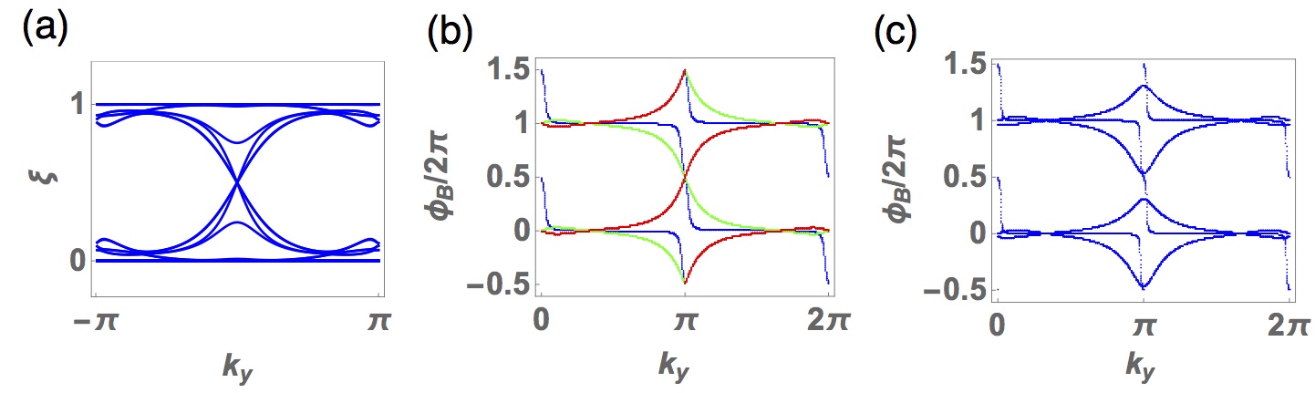
Figure 2: (a) Entanglement spectrum $\xi(k_{y})$ at $k_{x}=\pi$ for the bipartition along $z$ direction. (a)The Berry phase as a function of $k_{y}$ at $k_{z}=0$ for the lowest three occupier bands (Blue, Red, Green) with corresponding mirror eigenvalue $(++-)$. (b) The crossing between blue and red lines can be gapped by adding inversion breaking and $\mathcal{R}_{z}$ preserving term.

II.3 Quantum oscillations

In order to determine whether a Majorana Fermi surface exhibit quantum oscillations, we calculate the dispersion under magnetic field by projecting the Hamiltonian on the Majorana band.

$$\epsilon^{\rm M}_{\bf k,A}=\langle\phi^{\rm M}_{\bf k}|H(k,A)|\phi^{\rm M}_{\bf k}\rangle=\frac{1}{2}(\epsilon^{\rm e}_{{\bf k}-e{\bf A}}+\epsilon^{\rm h}_{{\bf k}+e{\bf A}}),$$ (124)

where $\epsilon^{\rm e}_{\bf k-eA}$ and $\epsilon^{\rm h}_{\bf k+eA}$ are the dispersion for electrons and holes bands that couple to the external gauge field with opposite signs. Although $\epsilon^{\rm M}_{\bf k,A}$ break gauge invariance,we checked that our results are independent of the gauge choice for spherical Fermi surfaces. A fully gauge invariant calculation under magnetic field require a background of skyrmion fluid. In the main text, Fig. 2(c), we show that the density of states arising from the Majorana band under magnetic field indeed have sharp and periodic features that resemble Landau levels. These calculations are done in a two dimensional system with the Landau gauge ${\bf A}=(0,Bx,0)$, giving rise to a perpendicular magnetic field ${\bf B}=\nabla\times{\bf A}=B\hat{z}$. Since gauge field breaks the translational invariance along $x$ direction, we inverse Fourier transform the Hamiltonian back to complex fermions and perform a real space calculation along $x$ direction and include the magnetic field using the Peierls substitution, $t_{ij}\rightarrow t_{ij}{\rm e}^{\int_{i}^{j}{\bf A}\cdot d{\bf l}}$. Since $k_{y}$ is still a good quantum number, the calculation reduces to one dimensional strip for a given $k_{y}$, which are then summed up within the one dimensional Brillouin zone. To gain further insight, we can consider a parabolic band for the dispersion

$$\epsilon^{\rm M}_{\bf k,A} \simeq \frac{1}{2}\Big{[}\frac{({\bf k}-e{\bf A})^{2}}{2m^{*}}+\frac{({\bf k}+e{\bf A})^{2}}{2m^{*}}\Big{]}$$ (125)

$$= \frac{|{\bf k}|^{2}+e^{2}|{\bf A}|^{2}}{2m^{*}}$$

Since the linear coupling term ${\bf k}\cdot{\bf A}$ cancels, the current operator $J_{\alpha}=\partial\epsilon^{\rm M}_{\bf k,A}/\partial A_{\alpha}|_{\bf A=0}=0$ vanishes. Nevertheless, the $A_{\alpha}^{2}$ term, responsible for Landau quantization is still present, which is responsible for the Landau level like features in the density of states. Since quantum oscillations are manifestations of the sharp and periodic features of the Landau levels, we anticipate that Majorana Fermi surface can also give rise to quantum oscillations.

III Robust Order-parameter isotropy in the presence of spin-orbit coupling.

One thing that might save the superconductor, is if it has a spin anisotropy, induced for example, by spin-orbit coupling. If such an anisotropy set up an easy plane for the vector $\hat{\bf n}$, then the system would reduce to a $U(1)$ order parameter, with stable vortices. However, the Free energy of the ground-state does not depend on the orientation of the order-parameter. This can be seen by integrating out the conduction electrons, writing the effective action (Free energy) as

$$F=-\frac{T}{2}\sum_{{\bf k},i\omega_{n}}{\rm Tr}\ln\left[-{\cal G}^{-1}[{\bf k},i\omega_{n}]\right]$$

where

$${\cal G}^{-1}[{\bf k},i\omega_{n}]=(i\omega_{n}-\epsilon_{f}({\bf k}))\mathbb{I}_{3\times 3}-\Sigma_{M}({\bf k},i\omega_{n})$$

Now the only dependence of $F$ on the order parameter orientation comes via the Majorana self energy $\Sigma_{M}$. In our model, this quantity is given by

$$\Sigma^{M}_{ab}({\bf k},\omega) = {\cal V}^{\dagger}\sigma^{a}({\bf s}_{{\bf k}}\cdot\vec{\sigma})\frac{1}{i\omega_{n}-\epsilon_{{\bf k}}+\mu\tau_{3}}({\bf s}_{{\bf k}}\cdot\vec{\sigma})\sigma^{b}{\cal V}$$ (126)

$$= s_{{\bf k}}^{2}{\cal V}^{\dagger}\frac{\sigma^{a}\sigma^{b}}{i\omega_{n}-\epsilon_{{\bf k}}+\mu\tau_{3}}{\cal V}$$ (127)

$$= \frac{s_{{\bf k}}^{2}V^{2}}{(i\omega_{n}-\epsilon_{{\bf k}})^{2}-\mu^{2}}\left[\delta^{ab}(i\omega_{n}-\epsilon_{{\bf k}})-\mu i\epsilon^{abc}\hat{n}_{c}\right]$$ (128)

$$= \Sigma_{0}({\bf k},i\omega_{n})\delta^{ab}-i\Sigma_{1}({\bf k},i\omega_{n})\epsilon^{abc}n_{c}$$ (129)

where ${\cal V}^{\dagger}{\cal V}=V^{2}$, ${\cal V}^{\dagger}\tau_{3}\vec{\sigma}{\cal V}=V^{2}\hat{\bf n}$. Notice how this self energy has complete mirror symmetry ($\Sigma_{M}(k_{x},k_{y},k_{z},i\omega_{n})=\Sigma_{M}(\pm k_{x},\pm k_{y},\pm k_{z},i\omega_{n})$), but it also contains an anisotropy dependent on the direction $\hat{\bf n}$. However, this does not produce any corresponding anisotropy in the free energy. To see this, lets look at the Free energy of the Majorana Fermions

$$F=-\frac{T}{2}\sum_{{\bf k},i\omega_{n}}{\rm Tr}\ln[(-i\omega_{n}+\epsilon_{f}({\bf k})+\Sigma_{0})\delta^{ab}+\Sigma_{1}({\bf k},i\omega_{n})i\epsilon^{abc}n_{c}].$$ (130)

Now we can always carry out a rotation in spin space inside the trace so that the n-vector points in the z-direction, and this rotation leaves the trace and hence the energy, unchanged. Since the Free energy that results has lost all information about the direction of the n-vector, it follows that the Free energy is isotropic. Lets see this in its engineering glory:

$$F = -\frac{T}{2}\sum_{{\bf k},i\omega_{n}}{\rm Tr}\ln\left[\begin{pmatrix}\epsilon_{fk}+\Sigma_{0}-i\omega_{n}&0&0\cr 0&\epsilon_{fk}+\Sigma_{0}-i\omega_{n}&-i\Sigma_{1}\cr 0&i\Sigma_{1}&\epsilon_{fk}+\Sigma_{0}-i\omega_{n}\end{pmatrix}\right]$$ (131)

$$= -\frac{T}{2}\sum_{{\bf k},i\omega_{n}}\ln\left[\epsilon_{fk}+\Sigma_{0}-i\omega_{n}\right]-\frac{T}{2}\sum_{{\bf k},i\omega_{n}}\ln\left[(\epsilon_{fk}+\Sigma_{0}-i\omega_{n})^{2}-\Sigma_{1}^{2}\right]$$ (132)

which has explicitly lost its dependence on the direction of $\hat{\bf n}$. We can thus be sure that even with a finite $\mu$ and spin-orbit coupling the mean-field Free energy is isotropic.

There will in general be a finite uniaxial anisotropy near the surface, where broken inversion symmetry develops. However, provided the bulk maintains cubic isotropy, the isotropy of the Free energy required for a higher order-parameter manifold is maintained at the mean-field level in the presence of spin-orbit coupling.