Classical Casimir interaction of perfectly conducting sphere and plate.

Abstract

We study the Casimir interaction between perfectly conducting sphere and plate in the classical limit of high temperatures. By taking the small-distance expansion of the exact scattering formula, we compute the leading correction to the Casimir energy beyond the commonly employed proximity force approximation. We find that for a sphere of radius $R$ at distance $d$ from the plate the correction is of the form $\ln^{2}(d/R)$, in agreement with indications from recent large-scale numerical computations. We develop a fast-converging numerical scheme for computing the Casimir interaction to high precision, based on bispherical partial waves, and we verify that the short-distance formula provides precise values of the Casimir energy also for fairly large distances.

I Introduction

Over the last two decades a new wave of precision experiments spurred a strong resurgence of interest in the Casimir effect Casimir48 , the tiny long-range force between (neutral) macroscopic polarizable bodies, due to quantum and thermal charge fluctuations within the bodies. For reviews we address the reader to Refs.book1 ; parse ; book2 ; woods .

A distinctive feature of the Casimir force is its non-additivity, a consequence of the inherent many-body character of fluctuation forces. This property enormously complicates the task of computing the Casimir force in arbitrary geometries. Indeed, Casimir himself was able to compute the force only for the highly idealized geometry of two perfectly conducting plane-parallel surfaces at zero temperature. A major step forward was made a few years later by Lifshitz lifs , who derived an exact formula for the Casimir interaction between two plane-parallel dielectric slabs at finite temperature. After these early successes in the planar geometry, the task of computing the force in non-planar geometries remained untractable for decades. This limitation has represented a serious practical problem because, in order to avoid the insurmountable parallelism issues posed by two plane-parallel surfaces separated by a sub-micron separation, practically all Casimir experiments adopt non planar geometries, like the sphere-plate. For a long time, the only tool to estimate the Casimir force between two non-planar gently curved surfaces has been the old-fashioned Proximity Force Approximation (PFA) Derjaguin , which expresses the Casimir force as the average of the plane-parallel force over the local separation between the surfaces. Being an uncontrollable approximation, the problem remained of addressing the systematic theoretical error engendered by the PFA, an issue of great importance for a proper interpretation of modern high precision Casimir experiments.

A breakthrough occurred in the early 2000’s when, generalizing early findings by Balian and Duplantier Balian and Langbein langbein , an exact scattering formula for the Casimir interaction between two (or more) dielectric objects of any shape was finally worked out sca1 ; sca2 ; kenneth . Shortly later, scattering formulae have been derived for the Casimir force and the power of heat transfer between two bodies at different temperatures bimontescat ; antezza1 ; krugertrace . At thermal equilibrium, the scattering formula has the form of a sum over so-called Matsubara (imaginary) frequencies of functional determinants involving the T-operators of the involved bodies. In principle, the formula allows to exactly compute the Casimir interaction between two bodies whose T-operators are either known (as it is the case for planes, spheres or cylinders emiguniversal ) or can be computed numerically (for example for periodic rectangular gratings lambrgrat ). Numerical schemes inspired by the scattering formalism have been developed over the last few years, by which it is now possible to estimate numerically with reasonable precision the Casimir force between objects with complicated shapes (see johnson and Refs. therein). Very recently, the scattering formula has been evaluated to yield the exact classical Casimir interaction between a sphere and a plate subjected to Drude (Dr) boundary conditions bimonteex1 , and between two perfectly conducting spheres in four Euclidean dimensions bimonteex2 .

The scattering formula undoubtedly constitutes a major advancement, however its practical utility has been limited so far because there is no known method to compute efficiently the T-operator for material surfaces of arbitrary shapes. Even in the few cases (spheres or cylinders) for which the scattering operator is known exactly, use of the scattering formula is hampered by its slow convergence rate. Consider as an example the experimentally important geometry of a metallic sphere of radius $R$ at a minimum distance $d$ from a plane. It has been found that to accurately compute the Casimir interaction, it is necessary to include in the scattering formula all multipoles up to an order $l_{\rm max}\gtrsim R/d$ or so. At the moment of this writing, the largest numerical computation lambrsphere has $l_{\rm max}=100$, which allows to estimate the Casimir interaction only for aspects ratios $d/R$ smaller than 0.02 or so. For comparison, it should be considered that in order to increase the magnitude of the force, Casimir experiments use a large sphere at small distances from the plate, with typical aspects ratios of the order of one thousandth. For so small aspect ratios, a precise computation of the Casimir interaction requires multipole orders of several thousands, which are out of reach for now.

From a practical standpoint, the main role of the exact scattering formula has perhaps been to serve as a guide towards systematically deriving approximation schemes in various regimes, going beyond the old PFA. For surfaces carrying corrugations of small amplitude, a systematic perturbative expansion of the Casimir interaction in powers of the small corrugation amplitude has been worked out lambrcorr . Several researchers have instead endeavored to compute curvature corrections to the Casimir interaction, in the experimentally important limit of small surface separations. This is clearly a problem of outmost practical importance, for the purpose of interpreting current small-distance precision experiments. There are presently two approaches to compute curvature corrections to the PFA. The first one consists in working out the asymptotic small-distance expansion of the exact scattering formula. The method is rigorous, but it has the drawback that the expansion has to be worked out ab initio for each model, and for each surface geometry. By following this route, the next-to-leading-order (NTLO) correction to the Casimir energy has been computed for the cylinder/plate and the sphere/plate geometries, initially for a free scalar field obeying Dirichlet (D) boundary conditions (bc) bordag1 , and then for the electromagnetic (em) field with perfect-conductor (P) bc bordag2 . Later the same approach was applied to a free scalar field obeying D, Neumann (N) and mixed ND bc on two parallel cylinders teo1 .

An alternative route to compute the NTLO correction to PFA assumes that the Casimir energy functional admits a derivative expansion (DE) in powers of derivatives of the surfaces height profiles. The coefficients of the DE are computed by matching the DE with the perturbative expansion of the Casimir-energy functional in the common domain of validity (for details see fosco1 ; bimonte1 ). An advantage offered by the DE, in comparison with the previous approach, is that once the DE is worked out for a specific model, it can be straightforwardly applied to surfaces of any shape. In fosco1 the DE was worked out for a D scalar field in the cylinder and sphere/plate geometries, giving results in agreement with the asymptotic small-distance expansion of the scattering formula in bordag1 . The DE for the em field with P bc, as well as for a scalar field obeying N and mixed DN bc was later worked out in bimonte1 , where the DE was also generalized to the case of two curved surfaces. Interestingly, the NTLO correction for the sphere/plate geometry with P bc obtained in bimonte1 by using the DE was in disagreement with the result reported in bordag2 : while the DE predicted an analytic correction $\sim d/R$, a larger logarithmic $\sim d/R\,\ln(d/R)$ correction had been found in bordag2 . A successive recalculation by some of the authors of bordag2 detected a sign mistake in their original computation, and finally led to full agreement with the DE expansion also in em and N cases. The DE for a D and N scalar at zero and finite temperature in any number of space-time dimensions was worked out in fosco2 , while the experimentally important case of dielectric curved surfaces at finite temperature is presented in bimonte2 . It is worth stressing that the NTLO correction predicted by the DE is also in full agreement with the short distance expansion of the exact sphere-plate and sphere-sphere classical Casimir energies both for Dr bc bimonteex1 as well as for P bc in four Euclidean dimensions bimonteex2 . The DE has been also used to study curvature effects in the Casimir-Polder interaction of a particle with a gently curved surface CPbimonte1 ; CPbimonte2 . The same method has been used very recently to estimate the shifts of the rotational levels of a diatomic molecule due to its van der Waals interaction with a curved dielectric surface CPbimonte3 .

In this paper we study the sphere-plate Casimir interaction for P bc, in the high-temperature (HT) or classical limit. In this limit, the Casimir interaction reduces to the zero-frequency Matsubara-term of the full finite-temperature scattering formula. The zero-frequency (i.e. the classical) term becomes dominant for sphere-plate separations $d$ that are larger than the thermal length $\lambda_{T}=\hbar c/(k_{B}T)$ ($\lambda_{T}=7.5$ microns at room temperature). A perfect conductor constitutes the idealized limit of a superconductor, i.e. a conductor with perfect Meissner effect bimontesuper . Ohmic metals are better modeled as Drude conductors, since normal metals do not impede static magnetic fields. Quite surprisingly, several short-distance precision experiments (see deccamag and Refs. therein) with metallic plates at room temperature are in better agreement with a superconductor-like model (i.e. the plasma model) for the dielectric function of the plates, while a single large distance experiment lamorth favors the Drude model. For a thorough discussion of this delicate problem we address the reader to the monograph book2 .

The HT limit of the Casimir interaction for P bc has been investigated in irina , where the asymptotic small distance expansion of the scattering formula was shown to reproduce in leading order the PFA. The authors of irina did not study though corrections to PFA. Determining the form of the the NTLO correction is an interesting problem, for the following reason. In the HT limit, the Casimir interaction for P bc is mathematically equivalent to the sum of the classical Casimir energies for a Dr or D scalar field (depending on whether the plates are grounded or not) plus a N scalar field. The HT limit of the sphere-plate Casimir interaction for D and Dr bc have been computed exactly not long ago bimonteex1 . However, the N and P cases have been intractable so far. Working out the NTLO correction to PFA for these two models is of great interest, because in the HT limit the perturbative kernels for N and P bc display a singular behavior for small in-plane momenta, invalidating the DE fosco2 ; bimonteex1 . The DE has been shown to fail also for the plasma model in the HT limit in foscopl . As a result, the analytic form of the NTLO for N and P bc is so far unknown. A large-scale numerical computation including up to 5000 partial waves antoine suggests a $\ln^{2}(d/R)$ form for the NTLO term. However, the data of antoine appeared to support a $\ln^{2}(d/R)$ also for the Dr model, and from the exact solution in bimonteex1 we now know that the correct NTLO correction for the Dr model is actually a $\ln(d/R)$ term, in accordance with the DE. To resolve the matter, it is clearly of interest to see if the NTLO for N and P bc can be worked out analytically. As we said above the DE cannot help now, and therefore we attacked the problem using the method based on the asymptotic expansion of the scattering formula bordag1 ; teo1 . We find that the NTLO is indeed of the $\ln^{2}(d/R)$ form as it was argued in antoine , and we determine its coefficient. We also develop an efficient numerical implementation of the exact scattering formula, based on the use of bispherical multipoles bimonteex1 . The fast convergence of our scheme allowed us to probe extremely small aspect ratios down to $d/R=10^{-5}$. We verify that the approximate formula obtained by taking the asymptotic short-distance expansion of the Casimir interaction is actually very accurate up to relatively large values of the aspect ratio.

The paper is organized as follows: in Sec II we discuss the HT limit of the scattering formula, and briefly review the exact HT sphere-plate solution for D and Dr bc of bimonteex1 . In Sec. III we compute the short-distance expansion of the HT scattering formula in the sphere-plate geometry for P bc, and we obtain an approximate formula for the Casimir interaction valid for small separations. By taking its short-distance limit, we compute explicitly the leading correction of the Casimir interaction beyond PFA. In Sec. IV we present a fast-convergent numerical scheme to compute the Casimir energy based on the use of bispherical multipoles, and compare our numerical results with the approximate formula derived in Sec. III. In Sec. V we present our conclusions.

II The Casimir energy in the classical limit

We start from the general scattering formula sca1 ; sca2 ; kenneth for the Casimir free energy of two objects (denoted as 1 and 2) in vacuum:

$${\cal F}=k_{B}T\sum_{n\geq 0}\,\!\!^{\prime}\,{\rm Tr\ln}[1-{\hat{M}}({\rm i}\,\xi_{n})]\;,$$

$${\hat{M}}={\hat{T}}^{(1)}{\hat{U}}{\hat{T}}^{(2)}{\hat{U}}\;.$$ (1)

Here $k_{B}$ is Boltzmann’s constant, $T$ is the temperature, $\xi_{n}=2\pi nk_{B}T/\hbar$ are the (imaginary) Matsubara frequencies, and the prime in the sum indicates that the $n=0$ term is taken with weight 1/2. In Eq. (1), ${\hat{T}}^{(j)}$ denotes the T-operator of object $j$, evaluated for imaginary frequency ${\rm i}\,\xi_{n}$, and ${\hat{U}}$ is the translation operator that translates the scattering solution from the coordinate of one object to the one of the other object. When considered in a plane-wave basis $|{\bf k},Q\rangle$, where ${\bf k}$ is the in-plane wave-vector and $Q=E,M$ is the polarization ($E$ and $M$ denote, respectively, transverse magnetic and transverse electric modes), the translation operator ${\hat{U}}$ is diagonal, with matrix elements $e^{-dq_{n}}$ where $d$ is the minimum distance between the objects, $q_{n}=\sqrt{k^{2}+\xi_{n}^{2}/c^{2}}$ with $k=|{\bf k}|$, and $c$ the speed of light. This shows that in the HT limit $k_{B}T\gg\hbar c/d$, the free energy is dominated by the first term $n=0$ in the sum Eq. (1):

$${\cal F}_{\rm HT}=-k_{B}T\;\Phi,\;\;\;\;\Phi=-\frac{1}{2}{\rm Tr\ln}[1-{\hat{M}}(0)]\;.$$ (2)

Here, $\Phi$ is a dimensionless temperature-independent function, depending on the static em response functions of the two bodies. Since the free-energy is proportional to the temperature, the HT (or classical) limit of the Casimir interaction has a purely entropic character.

We are interested in the classical Casimir interaction ${\cal F}_{\rm HT}$ of a sphere of radius $R$ placed at a (minimum) distance $d$ from a plate, bot subjected to P bc. We take the surface of the plate to coincide with the $(x,y)$ plane of a cartesian coordinate system, whose $z$ axis passes through the sphere center $C$ (see Fig.1). We define the aspect ratio $x$ of the system as $x=d/R$.

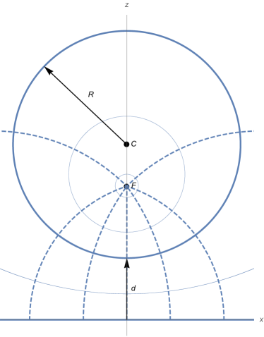
Figure 1: Geometry of a sphere and plate. Shown are the center $C$ of the sphere and its focus $F$. The system is characterized by its aspect ratio $x=d/R$. The thin solid and dashed lines correspond to curves of constant bispherical coordinates $\mu$ and $\eta$ respectively.

According to Eq. (2) the computation of ${\cal F}_{\rm HT}$ involves scattering of static em fields by the two surfaces. Static em fields with $E$ and $M$ polarizations represent, respectively, electrostatic and magnetostatic fields which do not mix under scattering by a dielectric surface of any shape. Therefore modes with $E$ and $M$ polarizations give separate contributions to the Casimir energy ${\cal F}_{\rm HT}$. Moreover, it is easily seen that in the static limit the em scattering problem is mathematically equivalent to the scattering problem for a free scalar field obeying the Laplace Equation. For perfect conductors, the bc obeyed by the scalar field are as follows. For $E$ polarization, the scalar field is subjected to either D or Dr bc on the surfaces of the two bodies, depending on whether the plates are grounded or not bimonteex1 ; foscoDr2 ; foscoDr , while for $M$ polarization the scalar field obeys N bc. The dimensionless function $\Phi^{\rm(P)}$ providing the classical Casimir interaction for P bc can be thus decomposed as the sum of two independent contributions $\Phi^{\rm(D/Dr)}$ and $\Phi^{\rm(N)}$, corresponding respectively to a D/Dr and a N scalar field:

$$\Phi^{\rm(P)}=\Phi^{\rm(D/Dr)}+\Phi^{\rm(N)}\;.$$ (3)

In the limit of vanishing separations $x$, the Casimir energy approaches the PFA limit:

$$\Phi^{\rm(D)}_{\rm PFA}=\Phi^{\rm(Dr)}_{\rm PFA}=\Phi^{\rm(N)}_{\rm PFA}=\frac{\Phi^{\rm(P)}_{\rm PFA}}{2}=\frac{\zeta(3)}{8\,x}\;.$$ (4)

The exact expression of the functions $\Phi^{\rm(D/Dr)}$ was determined in bimonteex1 by taking advantage of the separability of Laplace Equation in bisperical coordinates morse :

$$\Phi^{\rm(D)}=-\frac{1}{2}\sum_{l=0}^{\infty}(2l+1)\ln[1-Z^{2l+1}]\;,$$ (5)

$$\Phi^{\rm(Dr)}=-\frac{1}{2}\left\{\sum_{l=1}^{\infty}(2l+1)\ln[1-Z^{2l+1}]\;\right.$$

$$\left.+\ln\left[1-(1-Z^{2})\sum_{l=1}^{\infty}Z^{2l+1}\frac{1-Z^{2l}}{1-Z^{2l+1}}\right]\right\}\;,$$ (6)

where the parameter $Z$ depends on the aspect ratio $x$:

$$Z=[1+x+\sqrt{x\,(2+x)}]^{-1}\;.$$ (7)

The parameter $Z$ is less than one for all positive values of $x$, and as $x$ increases from 0 to $\infty$, $Z$ decreases monotonically from 1 towards zero.

Unfortunately, for N bc the Casimir interaction $\Phi^{\rm(N)}$ cannot be computed exactly. We find convenient to introduce the difference $\delta\Phi$ between the N and D energies $\Phi^{(N)}$ and $\Phi_{m}^{(D)}$:

$$\delta\Phi=\Phi^{(N)}-\Phi^{(D)}\;.$$ (8)

The energy for ungrounded perfect-conductors is accordingly represented as:

$$\Phi^{\rm(P)}=\Phi^{\rm(Dr)}+\Phi^{\rm(D)}+\delta\Phi\;,$$ (9)

while for grounded conductors we write:

$$\Phi^{\rm(P)}|_{\rm gr}=2\,\Phi^{\rm(D)}+\delta\Phi\;.$$ (10)

In the next Section we shall work out an asymptotic formula for $\delta\Phi$, valid in the limit of small separations, while in Sec. IV $\delta\Phi$ shall be computed numerically using the exact scattering formula Eq. (1).

III A short-distance formula for $\delta\Phi$

Before we start the computation of $\delta\Phi$, it is important to notice that, due to the presence of the trace in the general scattering formula Eq. (1), the Casimir interaction depends only on the equivalence class $[[M]]$ formed by all matrices $M$ that represent the operator ${\hat{M}}$, where two elements $M$ and $M^{\prime}$ of $[[M]]$ differ by a similarity transformation by an invertible matrix $A$: $M^{\prime}=AMA^{-1}$.

The matrix $M^{(\rm N)}$ for N bc is easily computed in a spherical multipole basis with origin at the sphere center $C$. In this basis the regular and outgoing eigenfunctions of the Laplace Equation have the familiar form $\phi_{lm}^{(\rm reg)}=r^{l}Y_{lm}(\theta,\phi)$, and $\phi_{lm}^{(\rm out)}=r^{-(l+1)}Y_{lm}(\theta,\phi)$, with $l\geq 0$, and $m=-l,\cdots,l$. By rotational symmetry around the azimuthal axis ${\hat{z}}$, the matrix $M^{(\rm N)}$ commutes with $J_{z}$ and hence is block diagonal. We let $M^{(\rm N|m)}$ the block corresponding to the value $m$ of $J_{z}$. One finds:

$${\hat{M}^{(\rm N|m)}}=\left[\left[\frac{l}{l+1}\,\frac{(l+l^{\prime})!}{(l+m)!(l^{\prime}-m)!}\left(\frac{1}{2(1+x)}\right)^{l+l^{\prime}+1}\right]\right]\;,$$ (11)

with $l,l^{\prime}\geq|m|$. Apart from the factor $l/(l+1)$, the matrix ${\hat{M}^{(\rm N|m)}}$ coincides with the corresponding matrix ${\hat{M}^{(\rm D|m)}}$ for D bc:

$${\hat{M}^{(\rm D|m)}}=\left[\left[\frac{(l+l^{\prime})!}{(l+m)!(l^{\prime}-m)!}\left(\frac{1}{2(1+x)}\right)^{l+l^{\prime}+1}\right]\right]\;,$$ (12)

Each block ${\hat{M}}^{(\rm N|m)}$ contributes separately to the Casimir energy, and we denote by $\Phi_{m}^{(N)}$ the corresponding contribution to $\Phi^{(N)}$. Of course, opposite values of $m$ give identical contributions to the Casimir energy, i.e. $\Phi_{m}^{(N)}=\Phi_{-m}^{(N)}$. We can thus write $\Phi^{(N)}$ as:

$$\Phi^{(N)}=2\sum_{m\geq 0}\,\!\!^{\prime}\Phi_{m}^{(N)}\;,$$ (13)

where the prime again denotes that the $m=0$ term is taken with a weight 1/2 and

$$\Phi_{m}^{(N)}=-\frac{1}{2}{\rm Tr\ln}[1-{\hat{M}}^{(\rm N|m)}]\;.$$ (14)

III.1 Contribution of the modes with $m=0$.

Luckily enough the contribution $\Phi_{0}^{(N)}$ of the $m=0$ modes can be computed exactly. By a similarity transformation with the diagonal matrix $A_{ll^{\prime}}=(l+1)\delta_{ll^{\prime}}$ the matrix ${M^{(\rm N|0)}}$ in Eq. (11) is transformed to the matrix ${\tilde{M}^{(\rm N|0)}}$

$${\tilde{M}^{(\rm N|0)}}_{ll^{\prime}}=\frac{l}{l^{\prime}+1}\,\frac{(l+l^{\prime})!}{l!\;l^{\prime}!}\left(\frac{1}{2(1+x)}\right)^{l+l^{\prime}+1}\;,$$ (15)

with $l,l^{\prime}\geq 0$. The first row of the matrix ${\tilde{M}}^{(\rm N|0)}$ is zero, while its $l$-th row with $l=1,2,\cdots$ is identical to the $(l-1)$-th row of the matrix $M^{(\rm D|0)}$ in Eq. (12) with its first column deleted: ${\tilde{M}}^{(\rm N|0)}_{ll^{\prime}}=M^{(\rm D|0)}_{l-1,l^{\prime}+1}$, $l=1,2,\cdots$, $l^{\prime}=0,1,2,\cdots$. By a second similarity transformation with the upper diagonal matrix ${\tilde{A}}(Z)$:

$${\tilde{A}}_{ll^{\prime}}(Z)=Z^{l^{\prime}-l}\frac{l^{\prime}!}{(l^{\prime}-l)!\;l!}\;,$$ (16)

with ${\tilde{A}}^{-1}(Z)={\tilde{A}}(-Z)$, the matrix ${\tilde{M}}^{(\rm N|0)}$ is transformed into a lower triangular matrix ${\bar{M}}^{(\rm N|0)}$, with diagonal elements equal to ${\bar{M}}^{(\rm N|0)}_{ll}=Z^{2l+3}$, $l=0,1,2,\cdots$. This implies at once:

$$\Phi_{0}^{(N)}=-\frac{1}{2}\sum_{l\geq 0}\ln[1-Z^{2l+3}]\;.$$ (17)

This result can be contrasted with the analogous formula for D bc bimonteex1 :

$$\Phi_{0}^{(D)}=-\frac{1}{2}\sum_{l\geq 0}\ln[1-Z^{2l+1}]\;.$$ (18)

III.2 Contribution of modes with $m\neq 0$.

Unfortunately, the contributions $\Phi_{m}^{(N)}$ of the modes with $m\neq 0$ cannot be computed exactly. By using the technique of Refs. bordag1 ; bordag2 ; teo1 it is however possible to prove a short-distance formula for $\Phi_{m}^{(N)}$, or more precisely for the difference $\delta\Phi_{m}=\Phi_{m}^{(N)}-\Phi_{m}^{(D)}$. We start by expanding the logarithm in Eq. (14):

$$\Phi_{m}^{(N/D)}=\frac{1}{2}\sum_{s=0}^{\infty}\frac{1}{s+1}\left(\prod_{i=0}^{s}\sum_{l_{i}=|m|}^{\infty}\right)\prod_{i=0}^{s}{M}^{(\rm N/D|m)}_{l_{i},l_{i+1}}\;,$$ (19)

where $l_{s+1}\equiv l_{0}$. Next, for $0<i\leq s$ we perform on the indices $l_{i}$ the shift: $l_{i}=l+l_{i}^{\prime}$, where we set $l:=l_{0}$. For small separations $x\ll 1$, the Casimir energy is dominated bordag1 ; bordag2 ; teo1 by multipoles such that:

$$l\sim 1/x\;,\;\;\;\;|l_{i}^{\prime}|\sim 1/\sqrt{x}\;,\;\;\;\;|m|\sim 1/\sqrt{x}\;.$$ (20)

For small $x$ the discrete sums over $l$ and $l_{i}^{\prime}$ in Eq. (19) can be replaced by integrations (this corresponds to taking the leading term in the Abel-Plana summation formula):

$$\Phi_{m}^{(N/D)}=\frac{1}{2}\int_{0}^{\infty}\!\!\!dl\;\left[{M}^{(\rm N/D|m)}_{l,l}\right.$$

$$\left.+\sum_{s=1}^{\infty}\frac{1}{s+1}\left(\prod_{i=1}^{s}\int_{-\infty}^{\infty}\!\!\!dl_{i}^{\prime}\right)\prod_{i=0}^{s}{M}^{(\rm N/D|m)}_{l+l_{i}^{\prime},l+l_{i+1}^{\prime}}\right]\;,$$ (21)

and we set $l_{0}^{\prime}=l_{s+1}^{\prime}\equiv 0$. In writing the above Equation, we considered that the integration over $l$ extending from $|m|$ to $\infty$ can be replaced by an integration from zero to $\infty$ because, according to Eq. (20), in the limit of small separations $m$ is negligibly small compared to $l$. We similarly replaced the integration over $l_{i}^{\prime}$ extending from $|m|-l$ to $\infty$ by an integration from $-\infty$ to $\infty$ because, compared to $l_{i}^{\prime}$, $(|m|-l)$ can be identified with $-\infty$. Next, we observe that by virtue of Eq. (20) the numbers $l+l^{\prime},l\pm m$ are all large integers for small $x$ and therefore the factorials in Eqs. (11) and (12) can be computed using Stirling’s formula:

$$\ln n!=\left(n+\frac{1}{2}\right)\ln n-n+\frac{1}{2}\ln 2\pi+\frac{1}{12n}+\cdots$$ (22)

At this point, we Taylor expand the difference $\delta{M}^{(\rm m)}_{l+l_{i}^{\prime},l+l_{i+1}^{\prime}}={M}^{(\rm N|m)}_{l+l_{i}^{\prime},l+l_{i+1}^{\prime}}-{M}^{(\rm D|m)}_{l+l_{i}^{\prime},l+l_{i+1}^{\prime}}$ among the matrices $M^{(N)}$ and $M^{(D)}$ in powers of $\sqrt{x}$ (powers of $\sqrt{x}$ are reckoned according to the estimates in Eqs. (20)). Up to terms of order $x^{2}$ we find:

$$\delta{M}^{(\rm m)}_{l+l_{i}^{\prime},l+l_{i+1}^{\prime}}=\frac{1}{\sqrt{4\pi l}}\left(\frac{l}{l+1}-1\right)\,\exp\left[-2xl-\frac{(l_{i}^{\prime}-l_{i+1}^{\prime})^{2}}{4l}-\frac{m^{2}}{l}\right]+o(x^{2})\;.$$ (23)

On the other hand, by taking the Taylor expansion of Eq. (12) we find:

$${M}^{(\rm D|m)}_{l+l_{i}^{\prime},l+l_{i+1}^{\prime}}=\frac{1}{\sqrt{4\pi l}}\exp{\left[-2xl-\frac{(l_{i}^{\prime}-l_{i+1}^{\prime})^{2}}{4l}-\frac{m^{2}}{l}\right]}+o(x)\;.$$ (24)

The two formulae above confirm correctness of the estimates in Eq. (20). There is a tricky but important point to stress here: following the logic of the Taylor expansion, one might find appropriate to replace the factor $[l/(l+1)-1]$ in the r.h.s. of Eq. (23) by its first order Taylor approximation $[l/(l+1)-1]=-1/l+o(x^{2})$. The problem with this substitution is that it leads to an infra-red divergence in the integral over $l$. To avoid this problem, we keep the complete factor $[l/(l+1)-1]$ in Eq.(23).

Starting from Eq. (21), and making use of Eqs. (23) and (24), we obtain the following expression for $\delta\Phi_{m}$:

$$\delta\Phi_{m}=\frac{1}{2}\int_{0}^{\infty}\frac{dl}{\sqrt{4\pi l}}\left\{\left(\frac{l}{l+1}-1\right)\exp\left(-2xl-\frac{m^{2}}{l}\right)+\frac{1}{2}\sum_{s=1}^{\infty}\frac{1}{s+1}\left[\left(\frac{l}{l+1}\right)^{s+1}-1\right]\right.$$

$$\left.\times\left(\prod_{i=1}^{s}\int_{-\infty}^{\infty}\frac{dl_{i}^{\prime}}{\sqrt{4\pi l}}\right)\prod_{i=0}^{s}\exp\left[-2\,x\,l-\frac{(l_{i}^{\prime}-l_{i+1}^{\prime})^{2}}{4l}-\frac{m^{2}}{l}\right]\right\}+o(x)\;,$$ (25)

Performing the gaussian integrals over $l_{i}^{\prime}$, we then obtain the following estimate for $\delta\Phi_{m}$ accurate to order $x^{1/2}$:

$$\delta\Phi_{m}^{(1/2)}=\frac{1}{2}\sum_{s=0}^{\infty}\frac{1}{(s+1)^{3/2}}\int_{0}^{\infty}\frac{dl}{\sqrt{4\pi l}}\left[\left(\frac{l}{l+1}\right)^{s+1}-1\right]\exp\left[(s+1)\left(-2\,x\,l-\frac{m^{2}}{l}\right)\right]\;.$$ (26)

The sum over $s$ can be expressed in terms the polylogarithm function ${\rm Li}_{n}(z)=\sum_{k=1}^{\infty}z^{k}/k^{n}$:

$$\delta\Phi_{m}^{(1/2)}=\frac{1}{2}\int_{0}^{\infty}\frac{dl}{\sqrt{4\pi l}}\left\{{\rm Li}_{3/2}\left[\frac{l}{l+1}\exp\left(-2\,x\,l-\frac{m^{2}}{l}\right)\right]-{\rm Li}_{3/2}\left[\exp\left(-2\,x\,l-\frac{m^{2}}{l}\right)\right]\right\}\;.$$ (27)

Combining the above formula with the exact expressions of $\Phi_{0}^{(N)}$ (Eq. (17)) and $\Phi_{0}^{(D)}$ (Eq. (18)) we obtain for $\delta\Phi$ the approximate small distance formula:

$$\delta\Phi^{(0)}=-\frac{1}{2}\sum_{l\geq 0}\ln\left(\frac{1-Z^{2l+3}}{1-Z^{2l+1}}\right)+2\sum_{m>0}\delta\Phi_{m}^{(1/2)}\;.$$ (28)

We expect that this formula for $\delta\Phi$ is accurate to order $x^{0}$. We shall later see that, despite the assumption $x\ll 1$ made in its derivation, the above formula provides a very precise value of $\delta\Phi$ also for relatively large separations (see Fig. 2).

III.3 Expressions at small distances

With exact expressions for the Casimir energies in the D and Dr models, one can compute explicitly the interaction in the limit of short distances $x\ll 1$. This limit corresponds to Z close to unity, and one can compute the series in Eqs. (5) and (6) using the Abel-Plana formula. We set $Z=\exp(-\mu)$, and then expand for small $\mu$, where $\mu=\ln[1+x+\sqrt{x\,(2+x)}]$. The resulting analytical expressions for the Casimir interaction were worked out in bimonteex1 , and we reproduce them here for the convenience of the reader:

$$\Phi^{(\rm D)}=\frac{\zeta(3)}{4\mu^{2}}-\frac{1}{24}\ln\mu-\frac{1}{16}+\gamma_{0}^{\prime}+\frac{7}{5760}\mu^{2}+o(\mu^{4})\;,$$ (29)

$$\Phi^{(\rm Dr)}=\Phi^{(\rm D)}-\frac{1}{2}\ln(\gamma_{1}-\ln\mu)-\frac{1}{12}\frac{\ln\mu-\gamma_{2}}{\ln\mu-\gamma_{1}}\mu^{2}+o(\mu^{4})\;,$$ (30)

with $\gamma_{0}^{\prime}=0.0874485$, $\gamma_{1}=1.270362$, $\gamma_{2}=1.35369$. We used $\mu$ as a variable for the expansion, for it provides a very accurate result also at larger distances. Both the D and Dr energies depend only on $\ln\mu$ and even powers of $\mu$. This implies that the energies depend only on $\ln x$ and integer powers of $x$. In particular, the force for the D case, once expanded in $x$, is a Laurent series starting from $1/x^{2}$. However, for the Dr case there are logarithmic terms in the force as well. The leading correction to PFA is the same $\ln\mu$ term for both models, and its coefficient is in agreement with the DE. Interestingly, for practically relevant separations the subleading double logarithmic term in Eq. (30) dominates over the leading logarithmic term, and therefore the D and Dr energies display rather different behaviors.

To work out the leading correction to PFA of the N energy, we start from Eq. (28). It is convenient to use for $\delta\Phi_{m}^{(1/2)}$ the expression in Eq. (26). In the limit of vanishing separation, the sum over the angular index $m$ can be replaced by an integration over $m$ extending from $-\infty$ to $\infty$. Performing the straightforward gaussian integral we find:

$$\delta\Phi_{\rm as}=\frac{1}{4}\sum_{s=0}^{\infty}\frac{1}{\!\!(s+1)^{2}}\int_{0}^{\infty}\!\!\!{dl}\left[\left(\frac{l}{l+1}\right)^{s+1}\!\!\!-1\right]e^{-2(s+1)xl}$$

$$=\frac{1}{4}\int_{0}^{\infty}\!\!\!{dl}\left[{\rm Li}_{2}\left(\frac{l}{l+1}e^{-2xl}\right)-{\rm Li}_{2}\left(e^{-2xl}\right)\right]\;.$$ (31)

We computed analytically the asymptotic expansion of the above formula for $x\rightarrow 0$ and found its leading term:

$$\delta\Phi_{\rm as}=-\frac{1}{16}\ln^{2}x+o(\ln x)\;.$$ (32)

Since in the D model the leading correction to the PFA is a $\ln x$ term (see Eq. (29)), the leading correction to the PFA for the N model coincides with the $\ln^{2}x$ term of $\delta\Phi$:

$$\Phi^{(N)}=\frac{\zeta(3)}{8\,x}-\frac{1}{16}\ln^{2}x+o(\ln x)\;.$$ (33)

Earlier we pointed out that the leading correction to the PFA for the Dr and the D model is the same $\ln x$ term. It then follows from Eq. (9) that the $\ln^{2}x$ term of $\Phi^{(N)}$ represents also the leading correction to the PFA for P bc:

$$\Phi^{(P)}=\frac{\zeta(3)}{4\,x}-\frac{1}{16}\ln^{2}x+o(\ln x)\;.$$ (34)

Thus our analytical results provide a rigorous proof of the $\ln^{2}(x)$ form of the leading curvature correction to PFA, in accordance with indications obtained from the high-precision numerical data of antoine .

IV Numerical computation of $\delta\Phi$

The HT limit of the (ungrounded) sphere-plate Casimir energy with P bc was computed in antoine by a large-scale numerical computation of the exact scattering formula Eq. (1) using the standard spherical basis with origin at the sphere center $C$. The computation in antoine included up to 5000 partial wave orders, which allowed the authors of Ref. antoine to accurately estimate the functions $\Phi^{\rm(P)}$ and $\Phi^{\rm(Dr)}$ for aspects ratios $x\geq 2\times 10^{-3}$.

Earlier we saw that the classical Casimir energy for ungrounded perfect conductors is the sum of the energies for a Dr scalar plus a N scalar (see Eq. (3)). The (normalized) energy $\Phi^{\rm(Dr)}$ can be computed exactly in the sphere-plate geometry (see Eq. (6)), while for N bc an exact formula exists for $m=0$ modes. In the previous Section we derived an asymptotic formula, Eq. (28), valid for small-distances, for the difference $\delta\Phi$ among the HT Casimir energies for N and D bc. In this Section the energy-difference $\delta\Phi$ is computed numerically, using the exact scattering formula Eq. (1). As we shall see, $\delta\Phi$ can be computed very efficiently by using a basis of bispherical multipoles bimonteex1 .

Bispherical coordinates $(\mu,\eta,\phi)$ morse are defined by $(x,y,z)=a(\sin\eta\cos\phi,\sin\eta\sin\phi,\sinh\mu)/(\cosh\mu-\cos\eta)$, where $a$ identifies the focus $F$ of the sphere defined by $\mu=\mu_{1}>0$ (see Fig.1). The sphere has radius $R=a/\sinh\mu_{1}$, and $L=a\coth\mu_{1}$ is the distance of its center $C$ from the $\mu=0$ plane. The Laplace Equation is separable in bispherical coordinates, and its regular and outgoing eigenfunctions are:

$$\phi_{lm}^{\rm reg/out}=\sqrt{\cosh\mu-\cos\eta}\,Y_{lm}(\eta,\phi)\exp[\pm(l+1/2)\mu]\;,$$ (35)

for $l\geq 0$, $m=-l,\cdots,l$. Relative to the sphere (plane) outgoing and regular eigenfunctions correspond, respectively to the upper (lower) and lower (upper) sign in the exponential. Scattering solutions can be expanded in these eigenfunctions. It is a simple matter to verify that in the bispherical basis of Eq. (35) the translation matrix $U$ is diagonal with elements $U_{lml^{\prime}m^{\prime}}=Z^{l+1/2}\delta_{ll^{\prime}}\delta_{mm^{\prime}}$. where $Z=\exp(-\mu_{1})$. For D bc the $T$-matrix for both the plane and sphere are minus the identity operator. Therefore, in the bispherical basis the $M^{\rm(D)}$ matrix for D bc is diagonal with elements $M^{\rm(D)}_{lml^{\prime}m^{\prime}}=Z^{2l+1}\delta_{ll^{\prime}}\delta_{mm^{\prime}}$, and thus evaluation of the scattering formula Eq. (1) is straightforward yielding the result quoted in Eq. (5). The case of Dr bc is more elaborate, as one has to remove the contribution of monopoles from the $m=0$ block. Details can be found in bimonteex1 . For N bc the $T$-matrix of the $\mu=0$ plane is equal to the identity operator. However, the $T$-matrix of the sphere is unfortunately non-diagonal. Of course, the $T$-matrix is still block diagonal with respect to the angular index $m$, and it is convenient to decompose its blocks as $T^{(2|m)}=1+\delta T^{(N|m)}$. By an explicit computation in the bispherical basis, it is found that the matrix $\delta T^{(N|m)}$ satisfies the linear system

$$B^{(m)}\;\delta T^{(N|m)}=-2\sinh\mu_{1}\;1\;,$$ (36)

where $B^{(m)}$ is the matrix of elements

$$B^{(m)}_{ll^{\prime}}=[(2l+1)\cosh\mu_{1}+\sinh\mu_{1}]\delta_{ll^{\prime}}$$

$$-(l-m)\delta_{l,l^{\prime}+1}-(l^{\prime}+m)\delta_{l+1,l^{\prime}}\;.$$ (37)

with $l,l^{\prime}\geq|m|$. The linear system Eq. (36) cannot be solved analytically, but it can be easily solved numerically after truncation in the multipole order $l,l^{\prime}<l_{\rm max}$.

At this point it would seem that nothing is really gained by using bispherical multipoles, because we still face the problem of computing determinants of infinite-dimensional matrices, as we had to do anyhow in the standard base of spherical multipoles. Indeed the situation seems even worse now, because earlier at least the matrix $M^{(N|m)}$ had a simple expression (see Eq. (11)), while now the matrix $\delta T^{(N|m)}$ has to be itself computed numerically by solving an infinite-dimensional linear system. This shortcoming of bispherical coordinates is however rewarded by the crucial advantage of a much faster rate of convergence with respect to the maximum value $l_{\rm max}$ of the multipole index $l$. To see this, consider the expression of the $M$ matrix for N bc in bispherical coordinates:

$$M^{(N|m)}_{ll^{\prime}}=Z^{2l+1}(\delta_{ll^{\prime}}+\delta T^{(m)}_{ll^{\prime}})\;,$$ (38)

with $l,l^{\prime}\geq|m|$. When this expression is substituted into the scattering formula Eq. (1), it is easy to factor out the D contribution, and one ends up with the following exact representation for the energy-difference $\delta\Phi$ defined in Eq. (2):

$$\delta\Phi=-\sum_{m\geq 0}\,\!\!^{\prime}\,{\rm Tr\log}[1+V^{(m)}\delta T^{(N|m)}]\;,$$ (39)

where $V^{(m)}$ is the diagonal matrix of elements:

$$V^{(m)}_{ll^{\prime}}=\frac{1}{1-e^{\mu_{1}(2l+1)}}\delta_{ll^{\prime}}\;.$$ (40)

The exponential in the denominator of $V^{(m)}_{ll^{\prime}}$ shows that the multipoles contributing to $\delta\Phi$ are those with $l,l^{\prime}\lesssim 1/\mu_{1}$. For small $x$, $\mu_{1}=-\ln Z=\ln[1+x+\sqrt{x\,(2+x)}]^{-1}\simeq\sqrt{2x}$ and then we see that the order $l$ of the relevant partial waves scales like $\sqrt{R/d}$, which is only the square root of the multipole order $l_{\rm max}\sim R/d$ (see Eq. (20)) needed in the spherical basis.

To demonstrate the fast rate of convergence of the scattering formula in bispherical coordinates, we take as an example $x=2\times 10^{-3}$, which is the smallest aspect ratio considered in antoine . By including in the scattering formula 5000 partial (spherical) waves, the authors of antoine computed $\Phi^{(\rm P)}=146.812$ and $\Phi^{(\rm Dr)}=74.5962$. On the other hand, using the exact formula in Eq. (5) we find $\Phi^{(\rm D)}=75.2936$. From Eq. (9) we then get $\delta\Phi=-3.07737$. In Table I we quote the values of $\delta\Phi$ obtained from Eq. (39) with inclusion of bispherical multipoles of order $l\leq l_{\rm max}$, for $l_{\rm max}=20,40,80,120$. As it can be seen, $\delta\Phi$ converges quickly, and already with $l_{\rm max}=80$ the error on $\delta\Phi$ is as small as $1.2\times 10^{-5}$. With $l_{\rm max}=120$ we reproduce the value computed in antoine using 5000 partial waves. It is interesting to compare the numerical value of $\delta\Phi$ with the estimate provided by the asymptotic formula Eq. (28). Evaluation of Eq. (28) gives $\delta\Phi^{(0)}=-3.068$, which differs from the numerical value of $\delta\Phi$ by less than 0.3 %.

${l_{\rm max}}$	20	40	80	120
$\delta\Phi$	-2.92435	-3.06243	-3.07725	-3.07737

Table 1: Numerical values of $\delta\Phi$ for aspect ratio $x=2\times 10^{-3}$ obtained from the scattering formula in bispherical coordinates Eq.(39) with inclusion of multipoles of order $l\leq l_{\rm lmax}$. The value of $\delta\Phi$ for $l_{\rm max}=120$ is in perfect agreement with the value obtained in antoine using spherical multipoles up to $l_{\rm max}=5000$.

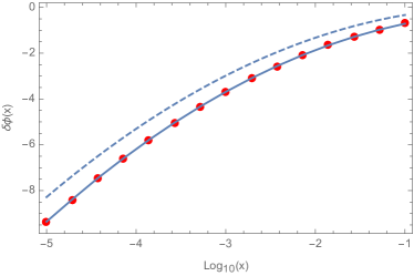
Figure 2: Difference $\delta\Phi=\Phi^{(\rm N)}-\Phi^{(\rm D)}$ among the sphere/plate N and D normalized Casimir energies as a function of $\log_{10}(x)$: numerical data (dots) computed using the scattering formula in a bispherical basis Eq. (39), small-distance formula Eq. (28) (solid line), leading term Eq. (32) (dashed line).

In Fig.2 we plot $\delta\Phi$ as a function $\log_{10}(x)$. The dots were computed using the scattering formula for $\delta\Phi$ in a bispherical basis Eq. (39). The fast convergence of Eq. (39) allowed us to accurately compute $\delta\Phi$ for aspect ratios as small as $x=10^{-5}$ by using less than 1000 partial waves. The solid line Fig.2 was computed using the asymptotic formula for $\delta\Phi$, Eq. (28). It can be seen that the asymptotic formula Eq. (28) provides a precise estimate of $\delta\Phi$ over the entire range of aspect ratios displayed in the Figure, up to the fairly large value $x=0.1$. The error made by using Eq. (28) varies from 0.16 % for $x=10^{-5}$ to a maximum of 1.2 % for $x=0.1$. The dashed line of Fig.2 corresponds to the leading term Eq. (32). By a fit procedure, we verified that a very good agreement between the dashed curve and the numerical data in Fig. 2 can be obtained by adding to the expansion in Eq. (34) a subleading logarithmic term proportional to $\ln x$.

A convenient representation of deviations from the PFA energy is provided by the function $\beta^{\rm(P)}(x)$ defined such that antoine :

$$\Phi^{\rm(P)}=-k_{B}T\,\frac{\zeta(3)}{4}\left(\frac{1}{x}+\beta^{(\rm P)}(x)\right)\;.$$ (41)

We similarly set:

$$\Phi^{\rm(D/Dr/N)}=-k_{B}T\,\frac{\zeta(3)}{8}\left(\frac{1}{x}+\beta^{(\rm D/Dr/N)}(x)\right)\;.$$ (42)

The exact expressions for the functions $\beta^{(\rm D/Dr)}(x)$ can be easily worked out starting from the exact solutions for the energies Eq. (5) and (6). On the other hand, $\beta^{(\rm N)}(x)$ can be expressed in terms of $\delta\Phi$:

$$\beta^{(\rm N)}(x)=\beta^{(\rm D)}(x)+\frac{8}{\zeta(3)}\,\delta\Phi\;.$$ (43)

Recalling Eq. (9), $\beta^{(\rm P)}(x)$ can be decomposed as:

$$\beta^{(\rm P)}(x)=\frac{1}{2}\left(\beta^{(\rm Dr)}(x)+\beta^{(\rm D)}(x)+\frac{8}{\zeta(3)}\,\delta\Phi\right).$$ (44)

In Fig. 3 we display a plot of $\beta^{\rm(P)}(x)$, where dots represent our numerical data, while the solid line is computed using the small-distance formula Eq. (28) for $\delta\Phi$.

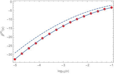
Figure 3: Additive correction $\beta^{\rm(P)}$ to the PFA classical Casimir energy for perfectly conducting sphere-plate as a function of $\log_{10}(x)$: numerical data (dots) computed using the scattering formula in a bispherical basis Eq. (39), small-distance formula for $\delta\Phi$ Eq. (28) (solid line), leading term for $\delta\Phi$ Eq. (32) (dashed line).

V Conclusions

We studied the Casimir interaction between a sphere and a plate, both perfectly conducting, in the classical limit of high temperatures. We worked out an analytical formula for the energy, valid for sufficiently small separations. Taking the asymptotic expansion of the small distance formula we found a $\ln^{2}(d/R)$ correction in the energy, beyond the commonly used proximity force approximation. The $\ln^{2}(d/R)$ form of the correction is in agreement with a fit of large-scale numerical data antoine . We developed a fast-converging numerical scheme for computing the Casimir energy, based on a system of bispherical partial waves. In bispherical coordinates, convergence of the exact scattering formula is achieved at multipole order $l_{\rm max}\simeq\sqrt{R/d}$, while in the standard approach based on spherical multipoles convergence is achieved only at order $l_{\rm max}\simeq R/d$. Using the bispherical basis, we could accurately compute the Casimir energy for very small aspects ratio $d/R=10^{-5}$. Comparison with the high precision numerical data shows that the analytical small-distance formula precisely estimates the energy also for fairly large values of the aspect ratio.

- (1) H. B. G. Casimir, Proc. K. Ned. Akad. Wet., 51, 793 (1948).
- (2) K. A. Milton, The Casimir Effect: Physical manifestations of Zero-Point Energy, World Scientific, Singapore (2001).
- (3) V. A. Parsegian, Van der Waals Forces, Cambridge University Press (2005).
- (4) M. Bordag, G. L. Klimchitskaya, U. Mohideen and V. M. Mostepanenko, Advances in the Casimir Effect, Oxford University Press (2009).
- (5) L. M. Woods, D.A.R. Dalvit, A. Tkatchenko, P. Rodriguez-Lopez, A.W. Rodriguez, and R. Podgornik, Rev. Mod. Phys. 88, 045003 (2016).
- (6) E. M. Lifshitz, Zh. Eksp. Teor. Fiz. 29, 94 (1955) [Sov. Phys. JETP 2, 73 (1956)].
- (7) B. Derjaguin, Kolloid Z. 69, 155 (1934)
- (8) R. Balian and B. Duplantier, Ann. Phys. 104, 300 (1977); ibid. 112, 165 (1978).
- (9) D. Langbein,Theory of van der Waals attraction, Springer (1974).
- (10) A. Lambrecht, P. A. Maia Neto and S. Reynaud, New J. Phys. 8, 243 (2006).
- (11) T. Emig, N. Graham, R. L. Jaffe, and M. Kardar, Phys. Rev. Lett. 99, 170403 (2007).
- (12) O. Kenneth and I. Klich, Phys. Rev. Lett. 97, 160401 (2006); Phys. Rev. B 78, 014103 (2008).
- (13) G. Bimonte, Phys. Rev. A 80, 042102 (2009).
- (14) R. Messina and M. Antezza, Phys. Rev. A 84, 042102 (2011).
- (15) M. Krüger, G. Bimonte, T. Emig, and M. Kardar, Phys. Rev. B 86, 115423 (2012).
- (16) S. J. Rahi, T. Emig, N. Graham, R. L. Jaffe, and M. Kardar, Phys. Rev. D 80, 085021 (2009).
- (17) A. Lambrecht and V. Marachevsky, Phys. Rev. Lett. 101, 160403 (2008).
- (18) S. G. Johnson, in Casimir Physics, Lecture Notes in Physics Vol. 834, edited by D. A. R. Dalvit, P. Milonni, D. Roberts, and F. da Rosa (Springer-Verlag, Berlin, 2011), p. 175.
- (19) G. Bimonte, T. Emig, Phys. Rev. Lett. 109, 160403 (2012).
- (20) G. Bimonte, Phys. Rev. D 94, 085021 (2016).
- (21) A. Canaguier-Durand, A. Gérardin, R. Guérout, P. A. Maia Neto, V. V. Nesvizhevsky, A. Yu. Voronin, A. Lambrecht, and S. Reynaud, Phys. Rev. A 83, 032508 (2011).
- (22) P. A. Maia Neto, A. Lambrecht and S. Reynaud, Phys. Rev. A 72, 012115 (2005).
- (23) M. Bordag and V. Nikolaev, J. Phys. A 41, 164002 (2008).
- (24) M. Bordag and V. Nikolaev, Phys. Rev. D 81, 065011 (2010).
- (25) L. P. Teo, Phys. Rev. D 84, 065027 (2011).
- (26) C. D. Fosco, F. C. Lombardo, and F. D. Mazzitelli, Phys. Rev. D 84, 105031 (2011).
- (27) G. Bimonte, T. Emig, R.L. Jaffe and M. Kardar, EPL 97, 50001 (2012).
- (28) C. D. Fosco, F. C. Lombardo, and F. D. Mazzitelli, Phys. Rev. D 86, 045021 (2012).
- (29) G. Bimonte, T. Emig, and M. Kardar, Appl. Phys. Lett. 100 074110 (2012).
- (30) G. Bimonte, T. Emig, and M. Kardar, Phys. Rev. D 90, 081702(R) (2014).
- (31) G. Bimonte, T. Emig, and M. Kardar, Phys. Rev. D 92, 025028 (2015).
- (32) G. Bimonte, T. Emig, R. L. Jaffe, and M. Kardar, Phys. Rev. A 94, 022509 (2016).
- (33) G. Bimonte, Phys. Rev. A 78, 062101 (2008).
- (34) G. Bimonte, D. Lopez, R. S. Decca, Phys. Rev. B 93, 184434 (2016).
- (35) A. O. Sushkov, W. J. Kim, D. A. R. Dalvit, and S. K. Lamoreaux, Nature Phys. 7, 230 (2011).
- (36) M. Bordag and I. Pirozhenko, Phys. Rev. D 81, 085023 (2010).
- (37) C. D. Fosco, F. C. Lombardo, and F. D. Mazzitelli, Phys. Rev. D 92, 125007 (2015).
- (38) A. Canaguier-Durand, G.-L. Ingold, M.-T. Jaekel, A. Lambrecht, P. A. Maia Neto, and S. Reynaud, Phys. Rev. A 85, 052501 (2012).
- (39) C. D. Fosco, F. C. Lombardo, and F. D. Mazzitelli, Phys. Rev. D 93, 125015 (2016)
- (40) C. D. Fosco, F. C. Lombardo, and F. D. Mazzitelli, Phys. Rev. D 94, 085024 (2016).
- (41) P.M. Morse and H. Feshbach, Methods of Theoretical Physics (McGraw-Hill, New York, 1953), Part II, p. 1298.