Algorithm for an arbitrary-order cumulant tensor calculation in a sliding window of data streams

Abstract

High order cumulant tensors carry information about statistics of non-normally distributed multivariate data. In this work we present a new efficient algorithm for calculation of cumulants of arbitrary order in a sliding window for data streams. We showed that this algorithms enables speedups of cumulants updates compared to current algorithms. This algorithm can be used for processing on-line high-frequency multivariate data and can find applications in, e.g., on-line signal filtering and classification of data streams. To present an application of this algorithm, we propose an estimator of non-Gaussianity of a data stream based on the norms of high-order cumulant tensors. We show how to detect the transition from Gaussian distributed data to non-Gaussian ones in a data stream. In order to achieve high implementation efficiency of operations on super-symmetric tensors, such as cumulant tensors, we employ the block structure to store and calculate only one hyper-pyramid part of such tensors.

Keywords: High order cumulants, time-series statistics, non-normally distributed data, data streaming.

1 Introduction

Cumulants of order one and two of $n$-dimensional multivariate data, i.e. mean vector and covariance matrix are widely used in signal and data processing, for example, in one of the most widely used algorithm in data and signal processing, namely Principal Component Analysis. Cumulants of order one and two describe completely statistically signal or data whose values are govern by a Gaussian distribution. In many real-life cases data or signals are not normally distributed. In this case it is necessary to employ higher order cumulants, such as, for example, skewness and kurtosis, to analyze this kind of data.

As the high order cumulant of $n$ dimensional multivariate data we understand the super-symmetric, cumulant tensor $\mathcal{C}\in\mathbb{R}^{[n,d]}$ of $d\geq 3$ modes, each of size $n$. Importantly they are zeros only if calculated for data sampled from multivariate Gaussian distribution [1, 2]. High order cumulants carry information about the divergence of the empirical distribution from the multivariate Gaussian one, hence we use them to extract such information from data.

Calculation of higher order cumulants for multi-dimensional data is time consuming. Furthermore, such data are often recorded in form of a stream and hence the on-line scheme of calculation and updates of cumulants is useful to analyze them. In this paper we present an efficient algorithm for calculation of cumulants of arbitrary order in a sliding window for data streams. We show the application of this algorithm to detect change in the underling distribution of multivariate time-series. Our algorithm uses so called block-structure, which is a data structure designed for efficient storage and processing of symmetric tensors.

1.1 Motivation

Our motivation to design such an algorithm comes from the fact that there exist many contemporary applications of higher order cumulants based algorithms in data processing. Typically these algorithms employ cumulants up to order four, and rarely up to order six. This limitation comes mainly from two factors: high computational cost of calculating higher order cumulants, and large amounts of data samples required to estimate faithfully higher order cumulants. Nowadays computational power is widely available and amounts of data collected every day is increasing dramatically. Therefore we believe that algorithms requiring usage of high order cumulants will be employed more widely in the near future. Yet, as it was pointed out by [3], processing data streams is a challenging task because it imposes constraints on memory usage, processing time, and number of data inputs reads. The algorithm presented in this work is dedicated to process efficiently on-line large data streams.

High order cumulants are used to analyze signal data, such as audio signals, for example in direction-finding methods of the multi-source signal (q-MUSIC algorithm) [4]. Additionally, high order cumulants are being used in signal filtering problems [5, 6] or neuroimaging signals analysis [7, 8]. The neuroscience application often uses the Independent Components Analysis (ICA) [9], that can be evaluated by means of high order cumulant tensors [10, 11]. Another important issue that requires fast algorithm to compute and update high order cumulants is financial data analysis, especially concerning high frequency financial data, where we deal with large data sets and the computational time is a crucial factor. For multi-assets portfolio analysis, high order cumulant tensors measures risk [12, 13], especially during a crisis where large fluctuations of assets values are possible [14, 15, 16].

While estimating high order statistics from data, there rises a problem of high estimation error. In general, large data set required for the accurate estimation of high order cumulants from data. This is discussed in [17] in some details. Unfortunately, large data set requires large computational time what becomes problematic if we want to analyze $n$-variate data on-line and $n$ is respectively large. To solve this problem we introduce an algorithm, that computes high order statistics in a sliding window of length $t$. Statistics are updated every time a new data batch of size $t_{\mathrm{up}}$ is collected.

The values of parameters $t$ and $t_{\mathrm{up}}$ depend on particular application. On one hand $t$ and $t_{\mathrm{up}}$ have to be large enough for an accurate approximation of the statistics, on the other hand the larger they are the weaker the time resolution of accessible for an application. We typically choose $t_{\mathrm{up}}=\alpha t$ with $\alpha=2.5\%,5\%,\ldots$ Given such parameters, we have reached over an order of magnitude speedup compared with a simple cumulants’ recalculation using fast algorithm introduced in [17]. In both cases we use the block structure [18] that allows to calculate and store efficiently super-symmetric cumulant and moment tensors [17]. We show that using the presented algorithm we can analyze data recorded at frequencies up to $2000$ Hz from $150$ Hz, depending in the number of marginal variables $n$: $60$—for the higher frequency figure to $120$—for the lower figure, on a modern six-core workstation.

1.2 Paper structure

The paper is organized as follows. In Section 2 we present formulas and algorithm employed to calculate cumulants of a data stream, the input data format, the sliding window mechanism, the block structure, moments tensors updates, cumulants calculation, and the complexity analysis. In Section 3 we discuss the algorithm implementation in Julia programming language, and the performance tests of the implementation. In Section 4 we introduce an illustratory application of our algorithm applied to analyze on-line the statistics of a data stream and analyze the maximal frequency of data that can be calculated on-line given a computer hardware.

2 Statistics updates

2.1 Data format

Let us consider the data that consists of $t$ realizations sampled from $n$-dimensional multivariate distribution forming an observation window whose number we will index by $w$:

$$\mathbb{R}^{t\times n}\ni\mathbf{X}^{(w)}=\begin{bmatrix}x_{1,1}^{(w)}&\dots&x_{1,n}^{(w)}\\ \vdots&\ddots&\vdots\\ x_{t,1}^{(w)}&\dots&x_{t,n}^{(w)}\\ \end{bmatrix}.$$ (1)

Note that samples form rows in the data matrix.

Further consider an update, that consists of another $t_{\mathrm{up}}$ $n$-dimensional realizations:

$$\mathbb{R}^{t_{\mathrm{up}}\times n}\ni\mathbf{X}_{(+)}^{(w)}=\begin{bmatrix}x_{t+1,1}^{(w)}&\dots&x_{t+1,n}^{(w)}\\ \vdots&\ddots&\vdots\\ x_{t+t_{\mathrm{up}},1}^{(w)}&\dots&x_{t+t_{\mathrm{up}},n}^{(w)}\\ \end{bmatrix},$$ (2)

that will be concatenated to $\mathbf{X}^{(w)}$ in order to form a new window. Additionally forming of a new window will require to drop first $t_{\mathrm{up}}$ realizations represented by the following matrix

$$\mathbb{R}^{t_{\mathrm{up}}\times n}\ni\mathbf{X}_{(-)}^{(w)}=\begin{bmatrix}x_{1,1}^{(w)}&\dots&x_{1,n}^{(w)}\\ \vdots&\ddots&\vdots\\ x_{t_{\mathrm{up}},1}^{(w)}&\dots&x_{t_{\mathrm{up}},n}^{(w)}\\ \end{bmatrix}.$$ (3)

The new observation window $w+1$ is given by the following equation

$$\begin{split}\mathbb{R}^{t\times n}\ni\mathbf{X}^{(w+1)}&=\begin{bmatrix}x_{t_{\mathrm{up}}+1,1}^{(w)}&\dots&x_{t_{\mathrm{up}}+1,n}^{(w)}\\ \vdots&\ddots&\vdots\\ x_{t+t_{\mathrm{up}},1}^{(w)}&\dots&x_{t+t_{\mathrm{up}},n}^{(w)}\\ \end{bmatrix}=\\ &=\begin{bmatrix}x_{1,1}^{(w+1)}&\dots&x_{1,n}^{(w+1)}\\ \vdots&\ddots&\vdots\\ x_{t,1}^{(w+1)}&\dots&x_{t,n}^{(w+1)}\\ \end{bmatrix}.\end{split}$$ (4)

The sliding window mechanism is visualized in Fig. 1.

Figure 1: Schematic representation of data flow in sliding window mechanism. In the picture the time flows from top to bottom. Subsequent windows are placed from left to right. Each multivariate data sample forms a row of a matrix.

2.2 Sliding window

The algorithm presented in this work calculates cumulants of a data stream in a sliding window. It is assumed that data arrive continuously to a system and are fed to the algorithm in typically small batches. The algorithm uses only a subset of current data stored in a buffer and minimal required statistics. As new data are incoming the calculations are performed on stored data and statistics. Historical data are iteratively discarded. The main loop is summarized in Algorithm 1. Which consists of the following steps: acquire new batch of data; calculate the oldest batch of data; update moments; calculate cumulants; update the data buffer.

Algorithm 1 Sliding window cumulant calculation algorithm

1:Input: $\mathbf{X}^{(1)}$ – first data batch

2:Output: $\mathcal{C}_{1}(\mathbf{X}^{(w)}),\ldots,\mathcal{C}_{d}(\mathbf{X}^{(w)})$ – cumulants for windows $1:w$

3:Calculate moments $\mathcal{M}_{1}(\mathbf{X}^{(1)}),\ldots,\mathcal{M}_{d}(\mathbf{X}^{(1)})$

4:$w\leftarrow 1$

5:for $w$ do

6:     Acquire $\mathbf{X}^{(w)}_{(+)}$.

7:     Calculate $\mathbf{X}^{(w)}_{(-)}$ from fist $t_{\mathrm{up}}$ rows of $\mathbf{X}^{(w)}$.

8:     $\mathcal{M}_{1}(\mathbf{X}^{(w+1)}),\ldots,\mathcal{M}_{d}(\mathbf{X}^{(w+1)})\leftarrow\text{momentsupdate}(\mathcal{M}_{1}(\mathbf{X}^{(w)}),\ldots,\mathcal{M}_{d}(\mathbf{X}^{(w)}),\mathbf{X}^{(w)}_{(+)},\mathbf{X}_{(-)}^{(w)})$

9:     $\mathcal{C}_{1}(\mathbf{X}^{(w+1)}),\ldots,\mathcal{C}_{d}(\mathbf{X}^{(w+1)})\leftarrow\text{mom2cums}(\mathcal{M}_{1}(\mathbf{X}^{(w+1)}),\ldots,\mathcal{M}_{d}(\mathbf{X}^{(w+1)}))$

10:     Calculate $\mathbf{X}^{(w+1)}$ by concatenating row by row $\mathbf{X}^{(w)}$ with $\mathbf{X}^{(w)}_{(+)}$ and remove rows belonging to $\mathbf{X}^{(w)}_{(-)}$.

11:     Emit $\mathcal{C}_{1}(\mathbf{X}^{(w+1)}),\ldots,\mathcal{C}_{d}(\mathbf{X}^{(w+1)})$.

12:     $w\leftarrow w+1$

13:end for

2.3 Block structure

Moments and cumulants are super-symmetric tensors, therefore we use block structure as introduced in [18] to compute and store them effectively. Using the such a block structure we store and compute only one hyper-pyramidal part of the super-symmetric tensor in blocks of size $b^{d}$, where $b$ is a parameter of the storage method. One advantage of the block structure is that it allows for efficient further processing of cumulants what was discussed in [17].

2.4 Moment tensor updates

Given data $\mathbf{X}\in\mathbb{R}^{t\times n}$ the super-symmetric moment tensor of order $d$: $\mathcal{M}_{d}(\mathbf{X})\in\mathbb{R}^{[n,d]}$ consists of the following elements:

$${}m_{\mathbf{i}}(\mathbf{X})=\frac{1}{t}\sum_{l=1}^{t}\left(\prod_{i_{k}\in\mathbf{i}}x_{l,i_{k}}\right).$$ (5)

where $\mathbf{i}=(i_{1},\ldots,i_{d})$ is element’s multi-index and $i_{1},\ldots,i_{d}\in 1:n$. A naive approach to calculate moments $\mathcal{M}\left(\mathbf{X}^{(w)}\right)$ would be to calculate all $m_{\mathbf{i}}(\mathbf{X}^{(w)})$ for each window $w$. But in order to reduce the amount of computation required to calculate moments in sliding windows we take advantage of the fact, that given $\mathbf{X}_{(-)}^{(w)}$ and $\mathbf{X}_{(+)}^{(w)}$ it is easy to update each element of the moment tensor using the following relation:

$$\begin{split}&m_{\mathbf{i}}\left(\mathbf{X}^{(w+1)}\right)=\frac{1}{t}\sum_{l=1+t_{\mathrm{up}}}^{t+t_{\mathrm{up}}}\left(\prod_{i_{k}\in\mathbf{i}}x_{l,i_{k}}^{(w)}\right)=\\ &=\frac{1}{t}\sum_{l=1}^{t}\left(\prod_{i_{k}\in\mathbf{i}}x_{l,i_{k}}^{(w)}\right)+\\ &+\frac{t_{\mathrm{up}}}{t}\left(\frac{1}{t_{\mathrm{up}}}\sum_{l=1+t}^{t+t_{\mathrm{up}}}\left(\prod_{i_{k}\in\mathbf{i}}x_{l,i_{k}}^{(w)}\right)-\frac{1}{t_{\mathrm{up}}}\sum_{l=1}^{t_{\mathrm{up}}}\left(\prod_{i_{k}\in\mathbf{i}}x_{l,i_{k}}^{(w)}\right)\right)=\\ &=m_{\mathbf{i}}\left(\mathbf{X}^{(w)}\right)+\frac{t_{\mathrm{up}}}{t}\left(m_{\mathbf{i}}\left(\mathbf{X}_{(+)}^{(w)}\right)-m_{\mathbf{i}}\left(\mathbf{X}_{(-)}^{(w)}\right)\right).\end{split}$$ (6)

We can write Eq. (6) using tensor notation in the following tensor form:

$$\begin{split}\mathcal{M}\left(\mathbf{X}^{(w+1)}\right)=&\mathcal{M}\left(\mathbf{X}^{(w)}\right)+\\ +&\frac{t_{\mathrm{up}}}{t}\left(\mathcal{M}\left(\mathbf{X}^{(w)}_{(+)}\right)-\mathcal{M}\left(\mathbf{X}^{(w)}_{(-)}\right)\right).\end{split}$$ (7)

Algorithm 2 momentsupdate()

1:Input: data – $\mathbf{X}_{(+)}^{(w)}\in\mathbb{R}^{t_{up}\times n}$, $\mathbf{X}_{(-)}^{(w)}\in\mathbb{R}^{t_{up}\times n}$, moments – $\mathcal{M}_{1}(\mathbf{X}^{(w)}),\ldots,\mathcal{M}_{d}(\mathbf{X}^{(w)})$.

2:Output: updated moments – $\mathcal{M}_{1}(\mathbf{X}^{(w+1)}),\ldots,\mathcal{M}_{d}(\mathbf{X}^{(w+1)})$

3:for $s\leftarrow 1:d$ do

4:     $\mathcal{M}_{s}(\mathbf{X}^{(w+1)})\leftarrow\mathcal{M}_{s}(\mathbf{X}^{(w)})+\frac{t_{\mathrm{up}}}{t}\left(\mathcal{M}\left(\mathbf{X}^{(w)}_{(+)}\right)-\mathcal{M}\left(\mathbf{X}^{(w)}_{(-)}\right)\right)$

5:end for$\triangleright$ See Eq. (7)

6:return $\mathcal{M}_{1}(\mathbf{X}^{(w+1)}),\ldots,\mathcal{M}_{d}(\mathbf{X}^{(w+1)})$

Exploiting this form we can write the Algorithm 2 which calculates moments in a sliding window $w+1$ given moments of window $w$, and the data batches $\mathbf{X}_{(-)}^{(w)}$ and $\mathbf{X}_{(+)}^{(w)}$.

There exists a different approach to this problem. We could calculate ${t}/{t_{\mathrm{up}}}$ moments of data batches and organize the moments in a FIFO queue

$$\left(\mathcal{M}\left(\mathbf{X}_{(+)}^{(w_{1})}\right),\mathcal{M}\left(\mathbf{X}_{(+)}^{(w_{2})}\right),\ldots,\mathcal{M}\left(\mathbf{X}_{(+)}^{(w_{{t}/{t_{\mathrm{up}}}})}\right)\right).$$ (8)

With arrival of new batch its moments would be calculated and added to the aggregate moments then the oldest batch moments would be subtracted from the aggregate. This scheme reduces the amount of calculations because it does not require to calculate moments of $\mathbf{X}_{(-)}^{(w)}$ for each window $w$, but requires the storage of ${t}/{t_{\mathrm{up}}}$ moments for data $\mathbf{X}_{(+)}^{(w_{b})}$ for $w_{b}\in w:w+{t}/{t_{\mathrm{up}}}$. Therefore in approach we propose we have traded some of the computational complexity for the reduction in memory size requirements.

The moment tensor computation and storage in the block structure is explained in details in [17] from where we can conclude that if $b\ll n$ and $d\ll n$ we need approximately $\frac{n^{d}}{d!}(d-1)t$ multiplications to compute $\mathcal{M}_{d}(\mathbf{X})$. Analogically, we need $\frac{n^{d}}{d!}(d-1)t_{\mathrm{up}}$ multiplications to compute $\mathcal{M}\left(\mathbf{X}_{(+)}^{(w)}\right)$ and the same number of multiplications to compute $\mathcal{M}\left(\mathbf{X}_{(-)}^{(w)}\right)$. Obviously a simple recalculation of $\mathcal{M}(\mathbf{X}^{(w+1)})$ would require $\frac{n^{d}}{d!}(d-1)t$ multiplications. Hence given $\mathcal{M}\left(\mathbf{X}^{(w)}\right)$ computed priorly, the theoretical speedup factor of the update compared with a simple recalculation of $\mathcal{M}\left(\mathbf{X}^{(w+1)}\right)$ would be:

$$\frac{\frac{n^{d}}{d!}(d-1)t}{\frac{n^{d}}{d!}(d-1)t_{\mathrm{up}}+\frac{n^{d}}{d!}(d-1)t_{\mathrm{up}}}=\frac{t}{2t_{\mathrm{up}}},$$ (9)

what is significant especially if $t_{\mathrm{up}}\ll t$. In next two subsections we are going to show how to use the moment update scheme to update cumulant tensors.

2.5 Cumulant updates calculation

Given the moment tensor update scheme, due to the recursive relation between moments and cumulants tensors [19], we can use this scheme to form a cumulants’ update algorithm. The recursive relation between cumulants and moments was discussed in details the previous work [17]. Here this relation is summarized in a form of Algorithm 3. This algorithm calculates cumulants’ tensors $\mathcal{C}_{s}(\mathbf{X})\in\mathbb{R}^{[n,s]}$ for orders $s\in\{1,2,\ldots,d\}$, given moments $\mathcal{M}_{1}(\mathbf{X}),\ldots,\mathcal{M}_{d}(\mathbf{X})$.

Algorithm 3 moms2cums()

1:Input: $\mathcal{M}_{1}(\mathbf{X}),\ldots,\mathcal{M}_{d}(\mathbf{X})$ – moments

2:Output: $\mathcal{C}_{1}(\mathbf{X}),\ldots,\mathcal{C}_{d}(\mathbf{X})$ – cumulants

3:for $s\leftarrow 1:d$ do

4:     $\mathcal{C}_{s}(\mathbf{X})\leftarrow\mathcal{M}_{s}(\mathbf{X})-\mathcal{A}$ $\triangleright$ Calculate elements of $\mathcal{A}$ using algorithm 4

5:end for

6:return $\mathcal{C}_{1}(\mathbf{X}),\ldots,\mathcal{C}_{d}(\mathbf{X})$

Algorithm 4 Calculation of symmetrized outer product

1:Input: $\mathbf{i}$ – multi-index of cumulant tensor, $s$ – order of cumulant being calculated, $\mathcal{C}_{1}(\mathbf{X})$, $\mathcal{C}_{2}(\mathbf{X})$, …, $\mathcal{C}_{s-1}(\mathbf{X})$ – cumulant tensors of lower orders

2:Output: $\mathcal{A}_{\mathbf{i}}$ – element of super-symmetric tensor $\mathcal{A}$

3:$\mathcal{A}_{\mathbf{i}}=0$

4:for $\sigma\leftarrow 2:s$ do

5:     calculate partitions of the set $1:s$ into $\sigma$ parts $\triangleright$ using Knuth’s algorithm [20, Section 7.2.1.4]

6:     for $\xi\in\text{partitions}$ do

7:         $\mathrm{a}\leftarrow 1$

8:         for $k\in\xi$ do

9:              $\mathrm{a}\leftarrow\mathrm{a}\times\mathcal{C}_{\mathbf{i}(k)}(\mathbf{X})$

10:         end for

11:         $\mathcal{A}_{\mathbf{i}}\leftarrow\mathcal{A}_{\mathbf{i}}+\mathrm{a}$

12:     end for

13:end for

2.6 Complexity analysis

Despite using cumulants–moment recursive relation form [17], there are important computational differences between the cumulants’ updated scheme proposed in this paper and cumulants calculation scheme proposed in [17], see Eq. (34) therein. In the first case:

1. we need much less arithmetic operations to update a moment tensor than in the second case since $t_{\mathrm{up}}\ll t$, but

2. we need slightly more computational power to compute $\mathcal{A}$ in Algorithm 4. In the first case we can not use central moments for $\mathcal{M}_{d}$ because in general updates affect the centering of the data. Hence in the first case the inner loop starting in line 6 of Algorithm 4 runs over all partitions, in contrary to the second case, where similar algorithm sums over partitions containing only elements of size $\geq 2$.

In order to analyze the computational complexity of sliding window cumulant calculation algorithm, we have to count the number of multiplications performed in line 9 of the Algorithm 4. This number is given by:

$${}\begin{split}\sum_{\sigma=1}^{d}S(d,\sigma)(\sigma-1)=&\\ =\sum_{\sigma=2}^{d}S(d,\sigma)(\sigma-1)\leq&(d-1)\sum_{\sigma=2}^{d}S(d,\sigma)<\\ <&(d-1)B(d),\end{split}$$ (10)

where $S(d,\sigma)>0$ is the number of partitions of set of size $d$ into $\sigma$ parts, i.e. the Stirling Number of the second kind [21]; the sum $\sum_{\sigma=1}^{d}S(d,\sigma)=B(d)$, is the Bell number [22], the number of all partitions of the set of size $d$. The upper limit $(d-1)B(d)$ will be used further to approximate the number of multiplications required.

The number of multiplications is reduced due to the use of the block storage of super-symmetric tensors. We need only to calculate approximately $\frac{n^{d}}{d!}$ tensor elements see [17]. Given a moment tensor $\mathcal{M}_{d}$ and cumulant tensors $\mathcal{C}_{1},\ldots,\mathcal{C}_{d-1}$ we can approximate number of multiplications to compute $\mathcal{C}_{d}$ by

$$\frac{n^{d}}{d!}(d-1)B(d).$$ (11)

Nevertheless it is important to notice, that there is some additional computational overhead in the implementation due to operations on relatively small blocks.

Referring to Eq. (9) in order to update a series of moments we need approximately:

$$\#N_{\mathrm{mup}}(d)\approx\sum_{k=1}^{d}2\frac{n^{k}}{k!}(k-1)t_{\mathrm{up}}$$ (12)

multiplications. Further according to Eq. (11) to compute a series of cumulant tensors given a series of moment tensors we need approximately:

$$\sum_{k=1}^{d}\frac{n^{k}}{k!}(k-1)B(k)$$ (13)

multiplications. Finally to update a series of cumulants we need

$${}\begin{split}\#N_{\mathrm{cup}}&\approx\sum_{k=1}^{d}2\frac{n^{k}}{k!}(k-1)t_{\mathrm{up}}+\sum_{k=1}^{d}\frac{n^{k}}{k!}(k-1)B(k)=\\ &=\sum_{k=1}^{d}2\frac{n^{k}}{k!}(k-1)(2t_{\mathrm{up}}+B(k))\end{split}$$ (14)

multiplications. In practice, we use cumulants’ orders of $d=4,5,6$, number of data $t>10^{5}$, batch size of $t_{\mathrm{up}}=\alpha t$, where $\alpha=2.5\%,5\%,\ldots$, and number of variables $n\gg d$. Further given that Bell number $B(d)$ rises rapidly with $d$ [22] the last term of the sum in Eq. (14) is dominant and hence the final number of multiplications can be approximated by:

$${}\#N_{cup}\approx\frac{n^{d}}{d!}(d-1)(2t_{\mathrm{up}}+B(d)).$$ (15)

Simple cumulant series recalculation using [17] requires approximately $\sum_{k=1}^{d}\frac{n^{k}}{k!}(k-1)t\approx\frac{n^{d}}{d!}(d-1)t$ multiplications. The final speedup factor compared with such recalculation is:

$$\frac{t}{2t_{\mathrm{up}}+B(d)}.$$ (16)

The first term in the denominator corresponds to Algorithm 2, while the second one to Algorithm 3. For analyzed parameters’ values the function momentsupdate() is more computationally costly in comparison with moms2cums() by a factor of $\frac{2t_{\mathrm{up}}}{B(d)}$. For example for $t_{\mathrm{up}}=25000$ and $d=4$ the this factors is of three orders of magnitude.

In the following Sections we present the computer implementation of the cumulants updates algorithm in Julia programming language, and performance tests.

3 Implementation and performance

3.1 Implementation

The sliding window cumulant calculation algorithm was implemented in Julia programming language [23, 24, 25] and provided on the Zenodo repository [26]. Our implementation uses the block structure provided in [27], and parallel computation via the function pmap() implemented in Julia programming language. For the parallel computation implementation we perform the following.

1. We use parallel implementation of moment tensor calculation introduced in [17], i.e. data are split into $p$ non-overlapping sub-series, where $p$ is a number of workers, next we compute moment tensors for each sub-series and combine them into a single moment tensor.

2. We have also parallelized the for loop in line 4 of Algorithm 4 using pmap() function which is one of the ways Julia programming language implements a parallel for. The advantage of this solution is that each term of that sum is super-symmetric and we can compute it using block structure. The disadvantage is that the sum has only $d-1$ elements hence for large number of workers we do not take full advantage of the parallel implementation.

Despite some inefficiencies of parallel implementation, we obtain large speedup due to multiprocessing what is presented below.

3.2 Performance tests

In what follows we present performance tests carried out mainly using multiple CPU cores. All tests were performed on a computer equipped with Intel(R) Core(TM) i7-6800K CPU @ 3.40GHz processor providing $6$ physical cores and $12$ computing cores with hyper-threading, and $64$ GB of random access memory.

We start with determining the optimal block size parameter $b$ of the block structure (see Subsection 2.3). This parameter has complex impact on the computational time. On the one hand the higher $b$, the more computational and storage redundancy while calculating moment tensors, due to larger diagonal blocks. On the other hand the lower $b$ the more computational overhead due to larger amount of operations performed on small blocks.

(a) $d=4,n=60$

(b) $d=4,n=120$

(c) $d=5,n=60$

Figure 2: Cumulants updates computational times for different block sizes $b$ and the multiprocessing implementation on $6$ workers.

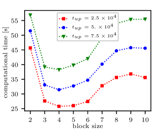
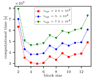
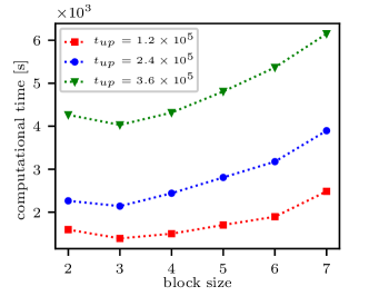
In Figure 2 we present the computational time of the update of cumulant tensors series of order $1,\ldots,d$ for different block sizes. One can observe that, the higher cumulant order $d$ the lower optimal block size $b$.

Finally fluctuations of computational time vs. block size are caused by the fact that, in our implementation, if $b$ does not divide $n$ some blocks are not hyper-squares and hence calculation of their size and block sizes conversion cause additional computational overhead. The computations of the optimal block size were performed using $6$ parallel worker processes.

Scalability of the algorithm with raising number of CPU cores is pretended in Figure 3.

(a) $d=4,n=120,b=4$

(b) $d=5,n=60,b=3$

Figure 3: Performance tests for multiprocessing implementation.

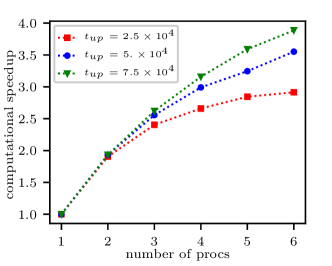
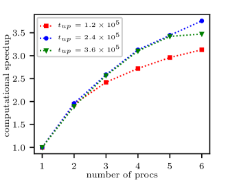
At first the computational time speedup is proportional to number of workers as it should be expected, however for large number of workers we do not fully take advantage of parallel implementation what is discussed in a previous section. Despite this problem we have still large speedup due to use multiple cores.

(a) $t=5\times 10^{5},d=4,b=4$.

(b) $t=1\times 10^{6},d=4,b=4$.

(c) $t=5\times 10^{6},d=5,b=3$.

(d) $t=25\times 10^{6},d=6,b=2$.

Figure 4: Speedup of cumulants updates comparing with [17] recalculation, $6$ workers implementation.

In Figure 4 we present the computational speedup of the update cumulants of order $1,\ldots,d$, compared with their simple recalculation [16] implemented in Julia [28]. The main conclusion is that the computational speedup is of about one order of magnitude. Higher speedup is recorded for large data sets.

4 Illustrative application

In this section we show a practical application of the sliding window cumulant calculation algorithm to analyze data that are updated in batches. As a simple application we propose the following scenario. The initial batch of data $\mathbf{X}^{(1)}$ is drawn from a multivariate Gauss distribution. Then the subsequent update batches $\mathbf{X}^{(w)}_{(+)}$ are drawn from $t$-Student copula—a strongly non-Gaussian distribution—having the same univariate marginal as the Gauss distribution. The transition from a Gaussian to a non-Gaussian regime is observed using the value of Froebenius norm of fourth cumulant tensor.

4.1 Cumulants based measures of data statistics

According to the definition of high order cumulants [1, 2] they are zero only if data are sampled from multivariate Gaussian distribution. Hence in this case the Frobenius norm of high order cumulant tensor:

$${}\|\mathcal{C}_{d}\|_{k}=\sqrt[k]{\sum_{\mathbf{i}}|c_{\mathbf{i}}|^{k}}$$ (17)

should be zero as well. Let us introduce a function

$${}\nu_{d}=\frac{\|\mathcal{C}_{d}\|_{2}}{\|\mathcal{C}_{2}\|_{2}^{d/2}}\text{ for }d>2,$$ (18)

that will be used to detect non-Gaussianity of data. Recall that in the case of univariate random variable, for $d=3$ and $d=4$ the function $\nu_{d}$ is equal to the modules of asymmetry and kurtosis. Obviously, for multivariate data, the higher values of $\nu_{d}$ the less likely that data were drawn from a multivariate Gaussian distribution.

Due to the use of block structure [18, 17] the function $\nu_{d}$ can be computed fast and use small amount of memory

Suppose we have the supper-symmetric cumulant tensor $\mathcal{A}\in\mathbb{R}^{[n,d]}$ stored in a block structure, i.e. we store only one hyper-pyramidal part of such tensor in blocks. Let $\mathbf{j}=(j_{1},\ldots,j_{d})$ be a multi-index of block $(\mathcal{A})_{\mathbf{j}}\in\mathbb{R}^{b^{d}}$, without loss of generality and for the sake of simplicity we assume that $b|n$. Then, in the block structure, we store only blocks indexed by such $\mathbf{j}$ whose elements are sorted in an increasing order.

We propose Algorithm 5 that computes a $k$-norm of given super-symmetric tensor $\mathcal{A}\in\mathbb{R}^{[n,d]}$. Blocks in a block structure can be super-diagonal (super-symmetric), partially diagonal (partially-symmetric) or off-diagonal.

Algorithm 5 Calculate $k$-norm of the tensor stored in a block structure.

1:Input: $\mathcal{A}\in\mathbb{R}^{[n,d]}$ – the supper–symmetric tensor stored in blocks, $\bar{n}$ – number of blocks

2:Output: Number – the $k$-norm of the tensor

3:$z\leftarrow 0$

4:for $j_{1}\leftarrow 1:\bar{n},\ldots,j_{d}\leftarrow j_{d-1}$ to $\bar{n}$ do

5:     $\mathbf{j}=(j_{1},\ldots,j_{d})$

6:     

$$z\leftarrow z+\frac{d!}{\prod_{l}r_{l}!}\sum_{e\in(\mathcal{A})_{\mathbf{j}}}|e|^{k}$$

$\triangleright$ $(\mathcal{A})_{\mathbf{j}}$ denotes a block indexed by multi-index $\mathbf{j}$

7:end for

8:return ${}^{k}\sqrt{z}$

Let $(\mathcal{A})_{\mathbf{j}}$ be an off-diagonal block, hence $j_{1}<j_{2}<\ldots<j_{d}$. In order to compute the Froebenius norm its elements must be counted $d!$ times in the sum since such block appears—up to generalized transpositions—$d!$ times in the in the full super-symmetric tensor. Since the Froebenius norm is an element-wise function, the order of tensor elements is not important.

In two other cases, partially diagonal or super-diagonal blocks have repeating indices—theirs multi-indices $\mathbf{j}$ are equal to:

$$\begin{split}(j_{1}<\ldots<\underbrace{j_{s_{1}}=\ldots=j_{s_{r_{1}}}}_{r_{1}}<\ldots<&\\ <\underbrace{j_{s_{2}}=\ldots=j_{s_{r_{2}}}}_{r_{2}}<\ldots&).\end{split}$$ (19)

Such blocks are repeated $\frac{d!}{\prod_{l}r_{l}!}$ times in the full tensor. Note that, if $j_{1}<j_{2}<\ldots<j_{d}$ then $\prod_{l}r_{l}!=1$. In the super-diagonal case i.e. $\mathbf{j}=(\underbrace{j_{1}=\ldots=j_{d}}_{d})$ we have:

$$\frac{d!}{\prod_{l}r_{l}!}=\frac{d!}{d!}=1,$$ (20)

so the super-diagonal block is counted only once as expected.

The advantage of Algorithm 5 is that it iterates over blocks in the block structure, what allows for efficient computation of the internal sum elements. A naive element-wise norm calculation approach would require $n^{d}$ power operations. To compute $\|\mathcal{A}\|$ using Algorithm 5 we need $b^{d}$ power operations for each block. Taking advantage of the block structure, required number of multiplications can be approximated by $\frac{n^{d}}{d!}$. Finally, the computational complexity of Algorithm 5 is small comparing with the computational complexity of Algorithm 2, the complexity of the procedure of cumulants updates and computation of their norms can be approximated by Eq. (15).

4.2 Data stream generation

In order to illustrate the functioning of aforementioned algorithms we use an artificially generated stream of data.

The initial data batch $\mathbf{X}^{(1)}\in\mathbb{R}^{t\times n}$ is sampled from a Gaussian multivariate distribution $\mathcal{N}(\mu,\Sigma)$, where ideally $\mu=\mathcal{C}_{1}(\mathbf{X}^{(1)})$, $\Sigma=\mathcal{C}_{2}(\mathbf{X}^{(1)})$. The subsequent data batches $\mathbf{X}^{(w)}_{(+)}\in\mathbb{R}^{t_{\mathrm{up}}\times n}$, for $w\geq 1$ are sampled from distribution $F$, which explained further. Our goal is to determine if the distribution of the updated data $\mathbf{X}^{(w)}\in\mathbb{R}^{t\times n}$ did not change with raising $w$, and is still a multivariate Gaussian.

A naive approach would be to compute the multiple univariate statistics, such as for example: asymmetry $\kappa_{3}$ and kurtosis $\kappa_{4}$ for each of the marginal variables of the data stream in windows $\mathbf{X}^{(w)}$ [29]. However such approach is oversimplified, since from the Sklar Theorem [30] one can deduce that it is always possible to construct such non-Gaussian multivariate distribution $F$ that has all marginal distributions $(F_{i})$ being univariate Gaussian. Hence despite $\forall_{i}\ \kappa_{3}(F_{i})=0,\kappa_{4}(F_{i})=0$, $F$ is not a multivariate Gaussian.

To generate such data in practice we can use a copula approach, see e.g. [31] for definition and formal introduction of copulas. The probability distribution $F$ is derived from the $t$-Student copula parametrized by $\Sigma$ and $\nu$ as defined in [31]. In our case we set the parameter to $\nu=10$ degrees of freedom and the marginals equal to those of $\mathbf{X}^{(1)}$.

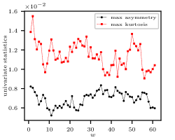
In order to visualize statistics of the generated data we calculate the maximums over marginals of absolute values of univariate asymmetries and kurtosises for $\mathbf{X}^{(w)}$. The results are presented in Fig. 5, as discussed before neither univariate asymmetry nor kurtosis is significantly affected by the update.

Figure 5: Maximums of absolute values of univariate asymmetries and kurtosises for $\mathbf{X}^{(w)}$ with number of marginal values $n=60$, $t=10^{6}$ data samples, $t_{\text{up}}=2.5\cdot 10^{4}$, $w_{\max}=61$.

4.3 Stream statistics analysis

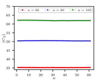
In order to detect the change in the probability distribution we calculate the following values of cumulants based measures in function of $w$. Those measures are $\|\mathcal{C}_{2}(\mathbf{X}^{(w)})\|$, $\nu_{3}(\mathbf{X}^{(w)})$ and $\nu_{4}(\mathbf{X}^{(w)})$, see Eq. (18). The obtained results are gathered in Fig. 6. Analyzing the panel 6(a) one can see that the norm of the covariance matrix is not significantly affected by the updates, this is due to the particular choice of the t-Student copula parameters [31] used to generate the updates.

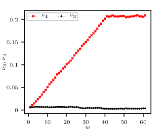
Further, as presented in panel 6(b) the $\nu_{3}(\mathbf{X}^{(w)})$ is also unaffected by updates, because t-Student copula is symmetric [31] in such a way that, given symmetric marginals, its high order odd cumulants are zero. However given t-Student copula this is not the case for even cumulants, e.g.$\nu_{4}(\mathbf{X}^{(w)})$ is strongly affected by updates and in this case can by used to distinguish between underling distributions from which data are drawn. The values of $\nu_{4}(\mathbf{X}^{(w)})$ raise with raising window number $w$, up to $w=41$, since for $w>41$ there is no original data from multivariate Gaussian distribution left in $\mathbf{X}^{(w)}$.

The normalization factor in the denominator of $\nu_{4}$ assures that the function behaves similarly for different number of marginal variables $n$. This behavior depends from the particular choice of the $t$-Student copula used in updates, however in general the choice of the particular measure $\nu_{d}$ should depend on the expected statistical model of a data stream.

Let us discuss the approximation error of $\nu_{4}(\mathbf{X})$. We assume that estimation error of $d$^th cumulant elements comes mainly from estimation error of corresponding $d$^th moment element. In an super-diagonal case, we can refer directly to Appendix $A$ in [17] and recall that the standard error of the estimation of $d$^th univariate moment $m_{d}$ is limited by $\sqrt{\frac{m_{2d}}{t}}$, in our case it is limited by $\sqrt{\frac{7!!}{10^{6}}}\approx 10^{-2}$. In a case of off-diagonal elements of $\mathcal{C}_{4}$, as mentioned in aforementioned Appendix $A$, estimation error is limited by the product of lower order moments which generally should by limited by $m_{2d}$, since moments’ values rise rapidly with $d$. Finally, while computing $||\mathcal{C}_{4}||$, see (17), we sum up squares of its elements, hence their individual errors should cancel out to some extend. However dependency between those elements is complex and a standard error calculus would be complicated. Hence we have performed $100$ numerical experiment, and computed for $n=100$ and $t=10^{6}$ $\nu_{4}$ from generated data. We obtained the following results summarized by the triplet of values: $5$^th quantile, median and $95$^th quantile of $\nu_{4}$ values. At $w=1$—Gaussian multivariate distribution—we have obtained $(0.004,0.006,0.011)$, while at $w\geq 41$—t-Student copula with Gaussian marginals—we have obtained $(0.199,0.209,0.220)$. In the second case the error is higher since the t-Student copula introduces high order dependencies between data and elements of $\mathcal{C}_{4}$. Concluding the estimation error is small in comparison with $\nu_{4}$ values.

(a) $\|C_{2}\|$,

(b) $\nu_{3}(\mathbf{X}^{(w)})\ \nu_{4}(\mathbf{X}^{(w)})\ n=100,$

Figure 6: Cumulants based statistical measures for data $\mathbf{X}^{(w)}\in\mathbb{R}^{t\times n}$, with window width $t=10^{6}$, update width $t_{\text{up}}=2.5\cdot 10^{4}$, and number of windows $w_{\max}=61$. The initial data are drawn from a Gaussian distribution, then the subsequent updates are drawn from a non-Gaussian one. We can observe that, in this case, $\nu_{4}$ is a good estimator of non-Gaussianity in contrast to function $\nu_{3}$. The value of $\nu_{4}$ raises with each window up to the saturation point at $w=41$.

4.4 Data frequency analysis

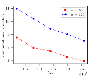
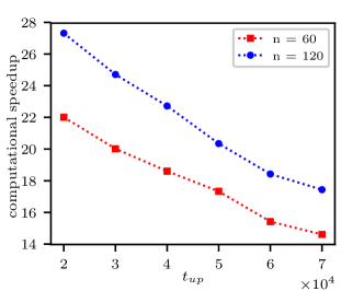
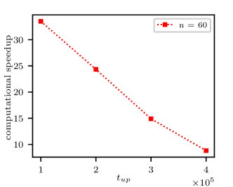
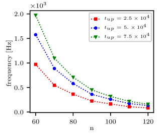
In order to estimate the maximal frequency of a data stream that can be analyzed on-line using Algorithm 1 we perform the following experiment using the same hardware discussed in Section 3.2. We fix the number of samples in a observation window $t$ and vary the number of marginals $n$ and number of samples in a batch $t_{\mathrm{up}}$. After the line 11 of Algorithm 1 is executed values of $\|\mathcal{C}_{1}(\mathbf{X}^{(w)})\|$, $\|\mathcal{C}_{2}(\mathbf{X}^{(w)})\|$, $\nu_{3}(\mathbf{X}^{(w)})$ and $\nu_{4}(\mathbf{X}^{(w)})$ are calculated.

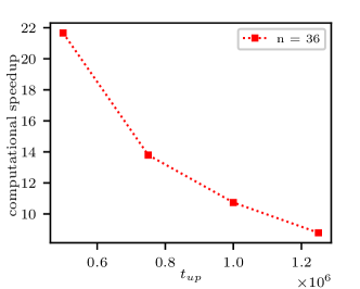
In Figure 7 we present the maximal frequency of data analyzed on-line using the proposed scheme. In presented example we compute and update cumulants of order $1,\ldots,4$ and use $\|\mathcal{C}_{1}(\mathbf{X}^{(w)})\|$, $\|\mathcal{C}_{2}(\mathbf{X}^{(w)})\|$, $\nu_{3}(\mathbf{X}^{(w)})$ and $\nu_{4}(\mathbf{X}^{(w)})$ to extract statistical features.

Consider that the Algorithm 4 for cumulants’ updates, is independent of $t_{\mathrm{up}}$ and therefore has constant execution time. Therefore one can increase maximal data frequency at the expanse of the method sensitivity by increasing $t_{\mathrm{up}}$.

Figure 7: Maximum frequency of on-line data analyzed using the cumulants updates scheme, $d=4$, $b=4$, multiprocessing computation on $6$ workers.

5 Conclusions

In this paper we have introduced a sliding window cumulant calculation algorithm for processing on-line high frequency multivariate data. For computer hardware described in Section 3 we have obtained maximum data processing frequency of $150$–$2000$ Hz depending on a number of marginal variables. We have presented an illustratory application of our algorithm by employing an example of Gaussian distributed data updated by data generated using t-Student copula. We have shown that our algorithm can be used successfully to determine if on-line updates break the Gaussian distribution.

We believe that presented algorithm can find many new applications for example in on-line signal filtering or classification of data streams. The algorithm can be combined with many different methods of the cumulant-based statistical features extractions, such as the Independent Component Analysis (ICA) [10, 11] or based on tensor eigenvalues [32].

References

- [1] M. G. Kendall et al., “The advanced theory of statistics,” The advanced theory of statistics., no. 2nd Ed, 1946.
- [2] E. Lukacs, “Characteristics functions,” Griffin, London, 1970.
- [3] J. Stefanowski, K. Krawiec, and R. Wrembel, “Exploring complex and big data,” Int. J. Appl. Math. Comput. Sci., vol. 27, no. 4, pp. 669–679, 2017.
- [4] P. Chevalier, A. Ferréol, and L. Albera, “High-Resolution Direction Finding From Higher Order Statistics: The -MUSIC Algorithm,” IEEE Transactions on signal processing, vol. 54, no. 8, pp. 2986–2997, 2006.
- [5] M. Geng, H. Liang, and J. Wang, “Research on methods of higher-order statistics for phase difference detection and frequency estimation,” in Image and Signal Processing (CISP), 2011 4th International Congress on, vol. 4, pp. 2189–2193, IEEE, 2011.
- [6] J. R. Latimer and N. Namazi, “Cumulant filters-a recursive estimation method for systems with non-Gaussian process and measurement noise,” in System Theory, 2003. Proceedings of the 35th Southeastern Symposium on, pp. 445–449, IEEE, 2003.
- [7] G. Birot, L. Albera, F. Wendling, and I. Merlet, “Localization of extended brain sources from EEG/MEG: the ExSo-MUSIC approach,” NeuroImage, vol. 56, no. 1, pp. 102–113, 2011.
- [8] H. Becker, L. Albera, P. Comon, M. Haardt, G. Birot, F. Wendling, M. Gavaret, C.-G. Bénar, and I. Merlet, “EEG extended source localization: tensor-based vs. conventional methods,” NeuroImage, vol. 96, pp. 143–157, 2014.
- [9] A. Hyvärinen, “Independent component analysis of images,” Encyclopedia of Computational Neuroscience, pp. 1–5, 2013.
- [10] T. Blaschke and L. Wiskott, “Cubica: Independent component analysis by simultaneous third-and fourth-order cumulant diagonalization,” IEEE Transactions on Signal Processing, vol. 52, no. 5, pp. 1250–1256, 2004.
- [11] J. Virta, K. Nordhausen, and H. Oja, “Joint use of third and fourth cumulants in independent component analysis,” arXiv preprint arXiv:1505.02613, 2015.
- [12] M. Rubinstein, E. Jurczenko, and B. Maillet, Multi-moment asset allocation and pricing models, vol. 399. John Wiley & Sons, 2006.
- [13] I. W. Martin, “Consumption-based asset pricing with higher cumulants,” The Review of Economic Studies, vol. 80, no. 2, pp. 745–773, 2013.
- [14] J. C. Arismendi and H. Kimura, “Monte Carlo Approximate Tensor Moment Simulations,” Available at SSRN 2491639, 2014.
- [15] E. Jondeau, E. Jurczenko, and M. Rockinger, “Moment component analysis: An illustration with international stock markets,” Swiss Finance Institute Research Paper, no. 10-43, 2015.
- [16] K. Domino, “The use of the multi-cumulant tensor analysis for the algorithmic optimisation of investment portfolios,” Physica A: Statistical Mechanics and its Applications, vol. 467, pp. 267–276, 2017.
- [17] K. Domino, Ł. Pawela, and P. Gawron, “Efficient computation of higer-order cumulant tensors,” SIAM J. SCI. COMPUT., vol. 40, no. 3, pp. A1590–A1610, 2018.
- [18] M. D. Schatz, T. M. Low, R. A. van de Geijn, and T. G. Kolda, “Exploiting symmetry in tensors for high performance: Multiplication with symmetric tensors,” SIAM Journal on Scientific Computing, vol. 36, no. 5, pp. C453–C479, 2014.
- [19] O. E. Barndorff-Nielsen and D. R. Cox, Asymptotic techniques for use in statistics. Chapman & Hall, 1989.
- [20] D. E. Knuth, The Art of Computer Programming, Volume 4A: Combinatorial Algorithms, Part 1, vol. 4. Addison-Wesley Professional, 2011.
- [21] R. L. Graham, D. E. Knuth, and O. Patashnik, “Concrete Mathematics: A Foundation for Computer Science,” Addison & Wesley, 1989.
- [22] L. Comtet, “Advanced combinatorics, reidel pub,” Co., Boston, 1974.
- [23] J. Bezanson, S. Karpinski, V. B. Shah, and A. Edelman, “Julia: A fast dynamic language for technical computing,” arXiv:1209.5145, 2012.
- [24] J. Bezanson, A. Edelman, S. Karpinski, and V. B. Shah, “Julia: A fresh approach to numerical computing,” SIAM Review, vol. 59, no. 1, pp. 65–98, 2017.
- [25] J. Bezanson, J. Chen, S. Karpinski, V. Shah, and A. Edelman, “Array operators using multiple dispatch: A design methodology for array implementations in dynamic languages,” in Proceedings of ACM SIGPLAN International Workshop on Libraries, Languages, and Compilers for Array Programming, p. 56, ACM, 2014.
- [26] K. Domino and P. Gawron, “CumulantsUpdates.jl,” Apr. 2018.
- [27] K. Domino, Ł. Pawela, and P. Gawron, “SymmetricTensors.jl,” Sept. 2017.
- [28] K. Domino, P. Gawron, and Ł. Pawela, “Cummulants.jl,” Feb. 2018.
- [29] J. Gama, Knowledge Discovery from Data Streams, vol. 20103856 of Chapman & Hall/CRC Data Mining and Knowledge Discovery Series. Chapman and Hall/CRC, May 2010.
- [30] A. Sklar, “Fonctions de répartition à n dimensions et leurs marges. publications de l’institut de statistique de l’université de paris,” 1959.
- [31] U. Cherubini, E. Luciano, and W. Vecchiato, Copula methods in finance. John Wiley & Sons, 2004.
- [32] L. Qi, “Eigenvalues of a real supersymmetric tensor,” Journal of Symbolic Computation, vol. 40, no. 6, pp. 1302–1324, 2005.