Contrast Agent Quantification by Using Spatial Information in Dynamic Contrast Enhanced MRI

Abstract

The purpose of this study is to investigate a method, using simulations, to improve contrast agent quantification in Dynamic Contrast Enhanced MRI. Bayesian hierarchical models (BHMs) are applied to smaller images ($10\times 10\times 10$) such that spatial information can be incorporated. Then exploratory analysis is done for larger images ($64\times 64\times 64$) by using maximum a posteriori (MAP).

For smaller images: the estimators of proposed BHMs show improvements in terms of the root mean squared error compared to the estimators in existing method for a noise level equivalent of a 12-channel head coil at 3T. Moreover, Leroux model outperforms Besag models. For larger images: MAP estimators also show improvements by assigning Leroux prior.

keywords: Contrast agent quantification, BHM, Besag, Leroux, INLA, MAP

1 Introduction

With dynamic contrast-enhanced MRI (DCE-MRI) the uptake and washout of a exogenous contrast agent (CA) can be monitored in certain tissues, e.g. tumors. By analysing the dynamics of the CA concentration using pharmacokinetics models (Sourbron and Buckley, 2013), it is possible to estimate physiology parameters such as blood flow, vessel density, capillary endothelial permeability, and extravascular extracellular space volume. These parameters are useful for characterizing e.g. tumor angiogenesis (Verma et al, 2012), performing target delineation and evaluating treatment response in radiotherapy (Cao, 2011).

A crucial step for successful parameter estimation is accurate determination of the CA concentration. This is difficult since the MR-signal have a complicated relationship to the CA concentration through the effect of the CA on the tissue relaxation time constants. Most commonly, CA concentration is estimated using the magnitude of the MRI images (Sourbron and Buckley, 2011), which is referred to as magnitude estimated CA in this paper. However, the accuracy of this method can be hampered by for instance issues like flip angle inhomogeneity (Cheng, 2007).

In addition to the magnitude information, MRI images also contain phase information. And the phase is influenced by the CA concentration. This has been exploited for accurate blood CA estimates and more recently Brynolfsson et al.. Brynolfsson et al (2014) combined magnitude and phase information to improve CA estimation in all types of tissue. In the work by Brynolfsson et al., a maximum likelihood estimator (MLE) was used to find the most likely CA concentration given noisy and biased magnitude images and noisy phase images. It is likely that CA concentration estimates can be improved even further if spatial (neighbor) information could be incorporated, since it is natural to assume that voxels next to each other behave alike, especially for the voxels in the same tissue.

The aim of this work is therefore to explore whether spatial information can provide further improvement by combining it with phase shift data and magnitude estimated CA. At current stage, we limit our evaluations to simulation data, since it is essential to establish the feasibility before trying to solve more difficult practical issues, such as the background phase drift.

The structure of the paper is organized as follows. The models with and without spatial information will be introduced in Section 2. In Section 3, the methods used in this work will be specified. Results will be presented in Section 4. The paper will be closed with conclusion and discussion.

2 Theory

2.1 Magnitude and phase models

This work uses the model developed by Brynolfsson et al. (Brynolfsson et al, 2014) as its starting point. Briefly, the model assumes that a measurement of the CA concentration $\mathbf{c}=(c_{1},...c_{N})$, where $N$ is the number of voxels in the image, is available from magnitude estimated CA data $\mathbf{c}_{m}=(c_{1},...,c_{N})$ and in addition to that also available from phase shift data $\Delta\mathbf{\varphi}=(\Delta\varphi_{1},...,\Delta\varphi_{N})$. The statistical model connecting the underlying CA concentration $\mathbf{c}$ and the measured data has the form

$$\mathbf{c}_{m} =D_{\boldsymbol{\xi}}\mathbf{c}+\boldsymbol{\epsilon}_{m}$$ (1)

$$\Delta\boldsymbol{\varphi} =\Psi\mathbf{c}+\boldsymbol{\epsilon}_{\varphi},$$ (2)

where $\boldsymbol{\epsilon}_{m}$, $\boldsymbol{\epsilon}_{\varphi}$ are two Gaussian white noise vectors and $D_{\boldsymbol{\xi}}$ is a diagonal matrix with diagonal elements $\boldsymbol{\xi}$ which is a Gaussian white noise vector with mean value $\mathbf{1}$. Thus, the magnitude estimated CA is both noisy and biased, while the phase shift data is only noisy. The matrix $\Psi$ represents a convolution and corresponds to how the magnetic properties of the CA perturb the measured phase shift data. An important feature of $\Psi$ is that it is singular and thus cannot be inverted. Equivalently, the matrix vector notation $(2)$ can be written voxel wise given by

$$\Delta\varphi(\mathbf{s})=F^{-1}(G(\mathbf{k})\cdot F(c(\mathbf{s})))+\epsilon_{\varphi}(\mathbf{s}),$$ (2*)

where $F$ is the Fourier transform function, $\mathbf{s}$ is the position vector in the image, $\mathbf{k}$ is the coordinate position vector in $k$-space and $G$ is a known function of $\mathbf{k}$ (Brynolfsson et al, 2014). Note that the drawback of $(2)$ compared with $(2^{*})$ is that $\Psi$ could be too huge to be stored into computer’s memory.

2.2 Model I: No spatial dependence

No spatial dependence is assumed to $\mathbf{c}$ in this model implying no spatial prior is added to the model $(1)$ and $(2)$ for $\mathbf{c}$. In this case $\mathbf{c}_{m}$ and $\Delta\boldsymbol{\varphi}$ are assumed to be independent between them and the MLE

$$\hat{\mathbf{c}} =\underset{\mathbf{c}}{\mathrm{argmin}}\left\{(\mathbf{c}_{m}-\mathbf{c})^{T}\Sigma_{m}^{-1}(\mathbf{c}_{m}-\mathbf{c})+(\Delta\boldsymbol{\varphi}-\Psi\mathbf{c})^{T}\Sigma_{\varphi}^{-1}(\Delta\boldsymbol{\varphi}-\Psi\mathbf{c})\right\}$$

is used to find $\mathbf{c}$ (Brynolfsson et al, 2014).

2.3 Model II: Bayesian hierarchical models (BHMs)

To incorporate spatial information into the model $(1)$ and $(2)$, BHM is used to model the spatial relationship. BHM is a statistical model consisting of multiple-stages. It estimates the parameters of interest by using Bayesian method. It is common to have three stages in the model. The first stage is data model used to model observed data, the second stage is process model used to model the unknown parameters of interest in data model and the last one is hyperparameter model used to model unknown hyperparameters. There are many well developed process models, e.g. Besag model (Besag et al, 1991), BYM model (Besag et al, 1991), Cressie model (Stern and Cressie, 2000) and Leroux model (Leroux et al, 2000), two of which are used in this work.

2.3.1 Besag model

Besag model is the simplest and most popular model, which has a special form of a generalized model (Besag, 1974) given by

$$\mathbf{c}\sim\mathcal{N}\left(\mathbf{0},\sigma^{2}(D(I-\rho W))^{-}\right),$$ (3)

where $\sigma^{2}$ is a variance parameter, $I$ is a identity matrix, $D=diag\left(d_{1},...,d_{N}\right)$ is a known diagonal matrix with $d_{i}$ is the number of neighbors of voxel $i$, $W=(W_{ij})$ is the proximity matrix,

$$W_{ij}=\begin{cases}1/d_{i},&i\sim j\\ 0,&\text{otherwise}\end{cases}$$

where $i\sim j$ indicates that the two voxels $i$ and $j$ are neighbors, - represents generalized inverse, and $\rho$ is a spatial dependence parameter. It can be shown that it suffices to let $\rho\in(1/\min_{i}\lambda_{i},1)$ to ensure the covariance matrix of $(3)$ to be positive definite, where $\lambda_{i},i=1,...,N,$ are eigenvalues of $W$ (Reber, 1999). However, since $\rho=1$ for Besag model, the covariance matrix of $(3)$ exists only in terms of generalized inverse.

In terms of full conditionals, the model $(3)$ can be expressed as

$$c_{i}|\mathbf{c}_{j|_{i\sim j}},\sigma,\rho\sim\mathcal{N}(\frac{\rho}{d_{i}}\underset{i\sim j}{\sum}c_{j},\frac{1}{d_{i}}\sigma^{2}),$$ (4)

where $\mathbf{c}_{j|_{i\sim j}}$ represents the elements which are neighbors of $c_{i}$. The conditional mean is affected by its neighbors, and conditional variance is proportional to the variance parameter $\sigma^{2}$. As mentioned above, $\rho=1$, thus there is no proper joint distribution from which $(4)$ can be derived. However, a sum to zero constraint, $\sum c_{i}=0$, can be added to $\mathbf{c}$ to guarantee the identifiability of this random field (Assunção and Krainski, 2009; Rue and Held, 2005). The inference process to obtain the estimates will be described in 2.3.3.

2.3.2 Leroux model

Although being invariant to the addition of any constant is a very important property (Rue and Held, 2005), Besag model has some undesired properties, e.g. the covariance matrix is not positive definite and it leads to a negative pairwise correlation for regions located further apart (MacNab, 2010). A proper prior is introduced here which was proposed by Leroux et al. (Leroux et al, 2000) and was the most appealing from both theoretical and practical standpoints (Lee, 2011). The joint distribution of Leroux model is given by

$$\mathbf{c}\sim\mathcal{N}\left(\mathbf{0},\sigma^{2}\left((1-\lambda)I+\lambda R\right)^{-1}\right),$$ (5)

where R is the structure matrix for Besag model which equals to $D(I-W)$, $\lambda$ is a spatial dependence parameter taking values within the interval of $(0,1)$. As $\lambda\to 1^{-}$, the model converges to Besag model and as $\lambda\to 0^{+}$, it converges to $\mathcal{N}(0,\sigma^{2}I)$.

In terms of full conditionals, the model of $(5)$ can be expressed as

$$c_{i}|\mathbf{c}_{j|_{i\sim j}},\sigma,\lambda\sim\mathcal{N}(\frac{\lambda}{1-\lambda+\lambda d_{i}}\underset{i\sim j}{\sum}c_{j},\frac{1}{1-\lambda+\lambda d_{i}}\sigma^{2}).$$

The major difference between the models in model I and model II is that $\mathbf{c}$ is considered as a deterministic unknown vector in model I while as a random unknown vector in model II by assuming it is a Gaussian Markov random field (GMRF).

2.3.3 INLA: Integrated nested Laplace approximations

To estimate the random unknown vector in BHMs, an algorithm based on INLA has been well developed. This method can be used for GMRFs which has been being applied in many scientific fields. The BHMs, described above, fit into this frame and are built with three stages. For simplicity reason, a new set of notations of random vectors is introduced, which has no connection with the notations existing before. The first stage is the data model $\pi(\mathbf{y|x}),$ where $\pi$ denotes probability density, $\mathbf{y}$ is the observation vector, $\mathbf{x}$ is the GMRF and $y_{i},i=1,...,N$, are independent conditional on $\mathbf{x}$. The second stage is the GMRF, $\pi(\mathbf{x}|\boldsymbol{\theta})$, where $\boldsymbol{\theta}$ is the hyperparameter vector and $\pi(\boldsymbol{\theta})$ is the third stage. INLA can provide accurate estimations for the GMRF and hyperparameters. The inference process is described briefly as follows:

The main interest is to estimate the marginal posterior distributions of the GMRF

$$\pi(x_{i}|\mathbf{y})=\int_{\boldsymbol{\theta}}\pi(x_{i}|\mathbf{y},\boldsymbol{\theta})\pi(\boldsymbol{\theta}|\mathbf{y})\mathrm{d}\boldsymbol{\theta},$$ (6)

of which the integrand can be obtained using approximations as follows.

$$\hat{\pi}(\boldsymbol{\theta}|\mathbf{y})\propto\frac{\pi(\mathbf{x,y,}\boldsymbol{\theta})}{\hat{\pi_{G}}(\mathbf{x|y,}\boldsymbol{\theta})}|_{\mathbf{x=x^{*}(\boldsymbol{\theta})}},$$

where the denominator $\hat{\pi_{G}}(\mathbf{x|y,}\boldsymbol{\theta})$ denotes the Gaussian approximation to the full conditional distribution of $\mathbf{x}$, and $x^{*}(\boldsymbol{\theta})$ is the mode of the full conditional of $\mathbf{x}$ for a given $\boldsymbol{\theta}$. Gaussian approximation means the distribution of a variable is approximated by a normal distribution by matching the mode and the curvature at the mode (Rue and Held, 2005).

The simplified Laplace approximation method is used to approximate the other component of the integrand of $(6)$ (Rue et al, 2009). This method is a trade off between accuracy and computational time and is commonly used in practice. It is also the default method in R-INLA. In order to perform a numerical integration of $(6)$, a number of good evaluation points $\boldsymbol{\theta}_{k}$ of $\boldsymbol{\theta}$ can be obtained by Newton like algorithms (Rue et al, 2009). Finally, an approximation of the posterior marginal density $(6)$ is given by

$$\pi(x_{i}|\mathbf{y})=\sum_{k}\hat{\pi}(x_{i}|\mathbf{y},\boldsymbol{\theta}_{k})\hat{\pi}(\boldsymbol{\theta}_{k}|\mathbf{y})\Delta\boldsymbol{\theta}_{k}$$

2.4 Maximum a posteriori (MAP)

Due to the limitation of R-INLA in this work describing in the next section, an exploratory analysis is done by using MAP estimator given by

$$\hat{\mathbf{c}} =\underset{\mathbf{c}}{\mathrm{argmin}}\left\{(\mathbf{c}_{m}-\mathbf{c})^{T}\Sigma_{m}^{-1}(\mathbf{c}_{m}-\mathbf{c})+(\Delta\boldsymbol{\varphi}-\Psi\mathbf{c})^{T}\Sigma_{\varphi}^{-1}(\Delta\boldsymbol{\varphi}-\Psi\mathbf{c})+\mathbf{c}^{T}Q\mathbf{c}\right\},$$ (7)

where $Q$ is the precision matrix of $\mathbf{c}$. Linear conjugate gradient algorithm is applied to find $\mathbf{c}$.

3 Methods

3.1 Data preparation

In this simulation study, the data was produced by using simulated GRE based DCE-MRI scans at 3T with a noise level equivalent of a 12-channel head coil (rSNR=5) and with a noise level of a 2-channel body coil (rSNR=1), respectively. rSNR is defined as rSNR$=\eta\cdot$SNR_bodycoil and $\eta\in[1,5]$. See Brynolfsson et al 2014 for details.

R-INLA is used to implement BHMs which has been mentioned in Section 2.3, however, it does not adapt for Fourier transform function used in $(2^{*})$, thus BHMs have to be applied to smaller images ($10\times 10\times 10$) such that $\Psi$ in $(2)$ can be stored into the computer’s memory. Then exploratory analysis is done for larger images ($64\times 64\times 64$) by utilising the estimates from smaller images. 30 simulations for smaller images and 50 simulations for larger images were produced and estimates of CA concentration were obtained with 2-second temporal resolution for the first 30 seconds and 5-second temporal resolution for the last 30 seconds. In other words, there are 22 time points for each simulation.

3.2 Common settings for all the models

Time is assumed to be independent. The covariance matrixes of $\boldsymbol{\epsilon}_{m}$ and $\boldsymbol{\epsilon}_{\varphi}$ are approximated from the simulated data, $\boldsymbol{\xi}$ is assumed to be $\mathcal{N}(1,0.09I)$ see Brynolfsson et al 2014 for details.

3.3 Specific settings for BHMs

$(1)$ and $(2)$ are used as data model. The prior for $\log(1/\sigma^{2})$ is set to be $\text{Log-Gamma}\left(1,5\times 10^{-5}\right)$ for Besag and Leroux models, which gives higher probability to relatively smaller variance. The prior for $\mathrm{logit}\lambda$ is set to be $\text{Logitbeta}(1,1)$ for Leroux model, which represents a non-informative prior.

The first order neighbourhood is used in proximity matrix. Two different assumptions are made to construct the proximity matrix $W$ for Besag model. The first is that two voxels next to each other are not neighbors if they are from different tissues. However, in reality we have no information about tissue classification, thus in the other case we do not give tissue restriction to $W$ that is two voxels next to each other are always neighbors. Only the second assumption is used for Leroux model. Under each assumption, the precision matrix Q has at most 6 non zero elements in the off-diagonal positions for each row such that Q is a very sparse matrix.

3.4 From smaller to larger images

Although we use R-INLA to analyze smaller images, larger images is used in clinic. MAP estimator is used for larger images with Leroux model for $\mathbf{c}$, which implies $Q^{-1}=\hat{\sigma}^{2}((1-\hat{\lambda})I+\hat{\lambda}R)^{-1}$ in $(7)$. By assuming that the spatial dependence $\lambda$ is invariant over different image sizes, the same estimates $\hat{\lambda}$’s for smaller images over the time points can be used. Note that full conditional variance $\text{Var}(c_{i}|\mathbf{c}_{-i})$ is proportional to $\hat{\sigma}^{2}$. Since the resolution of smaller images is lower than that of larger images, the full conditional variance of smaller images should smaller than that of larger images. Therefore, $\hat{\sigma}^{2}$ should be larger than the one in smaller images for each time point in general. Since the average precision $\hat{\tau}=1/\hat{\sigma}^{2}$ over 30 simulations for each time point could be calculated for smaller images, one can go through all possible values which are smaller than $\hat{\tau}$ to minimize $(7)$ for larger images. However, for the exploratory purpose, we set $\hat{\tau}$ to be a constant, which is smaller than the smallest averaged $\hat{\tau}$ over all the time points for smaller images, for larger images over all the time points.

To verify whether the spatial information can improve the estimation for lower rSNR, the same procedure is also applied to data produced with rSNR=1 at 3T. Since full conditional variance of the images with rSNR=1 should be larger than the one with rSNR=5, $\hat{\tau}$ should be smaller than the one with rSNR=5 for each time point in general. Again, a constant $\hat{\tau}$ for images with rSNR=1 is set for all the time points.

4 Results

4.1 Smaller images

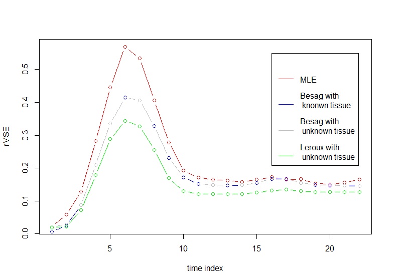
Figure 1: rMSE of vessels at 3T with rSNR=5

Figure 1 shows root mean squared error (rMSE) of vessels based on 30 simulations. From the figure, two Besag models show improvements in terms of rMSE, especially around the peak, where the percentage decrease is about 27%. And the Besag without tissue restriction is slightly worse than the one with tissue restriction, especially at the beginning of the time point. The mean difference between two Besag rMSE over 22 time points is about 0.001. The Leroux model outperforms the others. The improvements show both around the peak and right tail. It is about 40% decrease at the peak and 23% around the right tail compared to the MLE in model I.

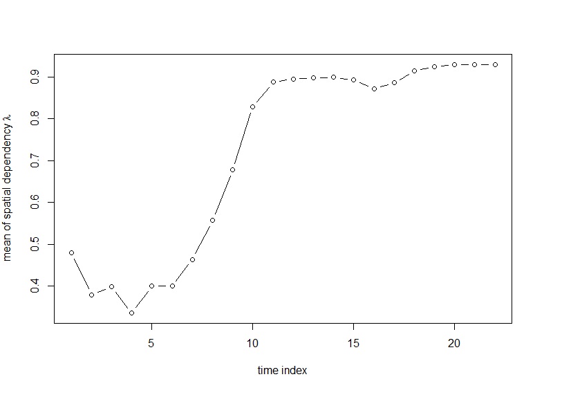
Figure 2: Time series of the mean of spatial dependence $\lambda$ at 3T with rSNR=5

From Figure 2, it shows apparently that the spatial dependence is negatively associated with CA concentration. The spatial dependence is lower when CA concentration is around the peak and the spatial dependence is getting higher when CA concentration is lower.

4.2 Larger images

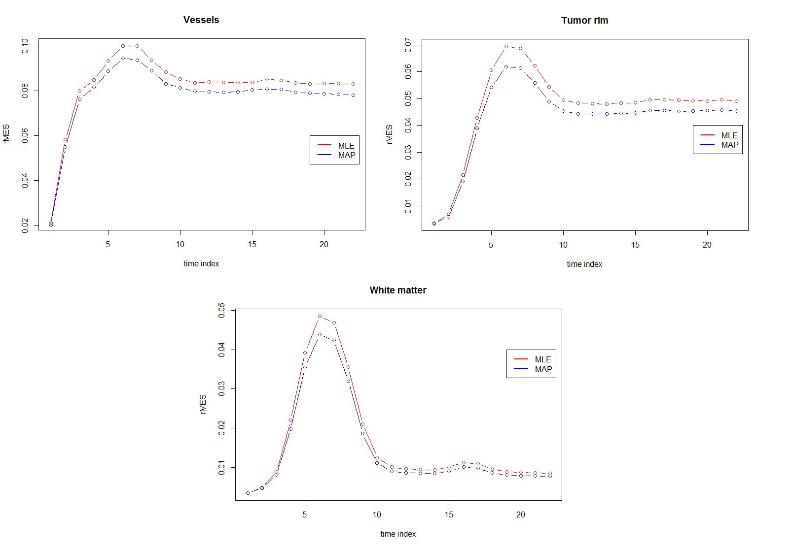
Figure 3: rMSE comparison between MAP estimators and MLEs for vessels, tumor rim and white matter at 3T with rSNR=5 over 50 simulations

Since the smallest averaged $\hat{\tau}$ for smaller images over all the time points is 0.9, $\hat{\tau}=0.1$ is selected to minimize $(7)$ for larger images. The same values shown in Figure 2 are used for $\hat{\lambda}$ to minimize $(7)$. From Figure 3, it shows both improvements around the peak and right tail for MAP estimators compared to MLEs over 50 simulations, even though $\hat{\sigma}^{2}$s are not the optimal ones to minimize $\mathbf{c}$ over time points.

The same analysis is done for the data produced with rSNR=1 at 3T. It shows that $\lambda$ has similar patten as in Figure 2. $\hat{\tau}=0.01$, which is less than 0.1, is selected for rSNR=1 at 3T.

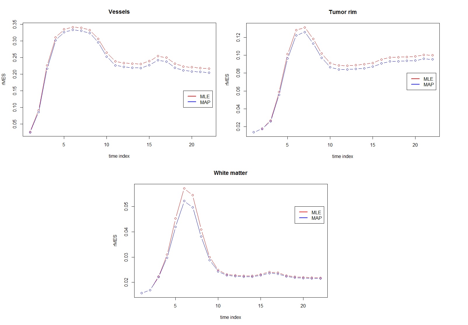
Figure 4: rMSE comparison between MAP estimators and MLEs for vessels, tumor rim and white matter at 3T with rSNR=1 over 50 simulations

Figure 4 is rMSE comparison between MAP estimators and MLEs with rSNR=1 at 3T and it also shows improvements compared to MLEs. Note that in general the rMSE in Figure 4 is larger than the one in Figure 3 due to the different noise levels.

5 Conclusion and Discussion

From the analysis above, it shows improvements by using spatial information in vessels for smaller images. And the Leroux model outperforms the Besag models. The MAP estimators are better than MLEs for vessels, tumor rim and white matter in terms of rMSE over 50 simulations for larger images with the assumption that spatial dependence is invariant over different image sizes, even though $\hat{\tau}$s are not optimal.

Although the smaller images are not practical in clinic, the results show clear evidences that borrowing strength from neighbors can improve the accuracy of CA concentration. The further analysis could be done in future by writing one’s own codes to implement BHMs for larger images instead of using R-INLA. In this case, with $(1)$ and $(2^{*})$ as the data model, Leroux model as the process model, one can check if the spatial dependence is invariant or not and how $\tau$’s change over different image sizes. Also different magnetic strength, e.g.1.5T, and more rSNRs can be analysed as in Brynolfsson et al (2014).

The other restriction of this study is that time dependence is not considered which results in a relatively simple statistical model and fast computational time. In reality, it is very reasonable to incorporate time dependence into the BHMs, which is called spatio-temporal BHMs (Cressie and Wikle, 2011). Figure 5 illustrates the spatio-temporal idea in a much concise way.

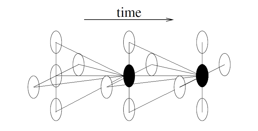
Figure 5: Neighborhood structure in spatio-temporal model

From the figure, the black dot is not only affected by its neighbors in space domain, but also by its neighbors in time domain. Many time series models can be used here, e.g random work models and autoregressive models. By incorporating the time dependence, besides temporal trend, the interaction between spatial and temporal effects can be studied.

References

- Assunção and Krainski (2009) Assunção R, Krainski E (2009) Neighborhood dependence in Bayesian spatial models. Biometrical Journal 51(5):851–869, DOI 10.1002/bimj.200900056, URL http://dx.doi.org/10.1002/bimj.200900056
- Besag (1974) Besag J (1974) Spatial interaction and the statistical analysis of lattice systems. Journal of the Royal Statistical Society Series B (Methodological) 36(2):192–236, URL http://www.jstor.org/stable/2984812
- Besag et al (1991) Besag J, York J, Molli A (1991) Bayesian image restoration, with two applications in spatial statistics. Annals of the Institute of Statistical Mathematics 43(1):1–20, DOI 10.1007/bf00116466, URL http://dx.doi.org/10.1007/BF00116466
- Brynolfsson et al (2014) Brynolfsson P, Yu J, Wirestam R, Karlsson M, Garpebring A (2014) Combining phase and magnitude information for contrast agent quantification in dynamic contrast-enhanced MRI using statistical modeling. Magn Reson Med 74(4):1156–1164, DOI 10.1002/mrm.25490, URL http://dx.doi.org/10.1002/mrm.25490
- Cao (2011) Cao Y (2011) The promise of dynamic contrast-enhanced imaging in radiation therapy. Seminars in Radiation Oncology 21(2):147–156, DOI 10.1016/j.semradonc.2010.11.001, URL http://dx.doi.org/10.1016/j.semradonc.2010.11.001
- Cheng (2007) Cheng HLM (2007) T1 measurement of flowing blood and arterial input function determination for quantitative 3D T1-weighted DCE-MRI. Journal of Magnetic Resonance Imaging 25(5):1073–1078, DOI 10.1002/jmri.20898, URL http://dx.doi.org/10.1002/jmri.20898
- Cressie and Wikle (2011) Cressie N, Wikle CK (2011) Statistics for Spatio-Temporal Data. Wiley, URL http://www.amazon.com/Statistics-Spatio-Temporal-Data-Noel-Cressie/dp/0471692743%3FSubscriptionId%3D0JYN1NVW651KCA56C102%26tag%3Dtechkie-20%26linkCode%3Dxm2%26camp%3D2025%26creative%3D165953%26creativeASIN%3D0471692743
- Lee (2011) Lee D (2011) A comparison of conditional autoregressive models used in Bayesian disease mapping. Spatial and Spatio-temporal Epidemiology 2(2):79–89, DOI 10.1016/j.sste.2011.03.001, URL http://dx.doi.org/10.1016/j.sste.2011.03.001
- Leroux et al (2000) Leroux BG, Lei X, Breslow N (2000) Estimation of Disease Rates in Small Areas: A new Mixed Model for Spatial Dependence, Springer New York, chap Statistical Models in Epidemiology, the Environment, and Clinical Trials, pp 179–191. DOI 10.1007/978-1-4612-1284-3˙4, URL http://dx.doi.org/10.1007/978-1-4612-1284-3_4
- MacNab (2010) MacNab YC (2010) On Gaussian Markov random fields and Bayesian disease mapping. Statistical Methods in Medical Research 20(1):49–68, DOI 10.1177/0962280210371561, URL http://dx.doi.org/10.1177/0962280210371561
- Reber (1999) Reber DL (1999) Inference for extremes with applications to animal breeding and disease mapping. Retrospective Theses and Dissertations p 12160
- Rue and Held (2005) Rue H, Held L (2005) Gaussian Markov Random Fields : Theory and Applications. Chapman & Hall/CRC
- Rue et al (2009) Rue H, Martino S, Chopin N (2009) Approximate Bayesian inference for latent Gaussian models by using integrated nested Laplace approximations. Journal of the Royal Statistical Society: Series B 71(2):319–392, DOI 10.1111/j.1467-9868.2008.00700.x, URL http://dx.doi.org/10.1111/j.1467-9868.2008.00700.x
- Sourbron and Buckley (2011) Sourbron SP, Buckley DL (2011) Tracer kinetic modelling in MRI: estimating perfusion and capillary permeability. Physics in Medicine and Biology 57(2):R1–R33, DOI 10.1088/0031-9155/57/2/r1, URL http://dx.doi.org/10.1088/0031-9155/57/2/R1
- Sourbron and Buckley (2013) Sourbron SP, Buckley DL (2013) Classic models for dynamic contrast-enhanced MRI. NMR Biomed 26(8):1004–1027, DOI 10.1002/nbm.2940, URL http://dx.doi.org/10.1002/nbm.2940
- Stern and Cressie (2000) Stern HS, Cressie N (2000) Posterior predictive model checks for disease mapping models. Statistics in Medicine 19(17-18):2377–2397, DOI 10.1002/1097-0258(20000915/30)19:17/18¡2377::aid-sim576¿3.0.co;2-1, URL http://dx.doi.org/10.1002/1097-0258(20000915/30)19:17/18<2377::AID-SIM576>3.0.CO;2-1
- Verma et al (2012) Verma S, Turkbey B, Muradyan N, Rajesh A, Cornud F, Haider MA, Choyke PL, Harisinghani M (2012) Overview of dynamic contrast-enhanced MRI in prostate cancer diagnosis and management. American Journal of Roentgenology 198(6):1277–1288, DOI 10.2214/ajr.12.8510, URL http://dx.doi.org/10.2214/AJR.12.8510