Nonlocal birth-death competitive dynamics with volume exclusion

Abstract

A stochastic birth-death competition model for particles with excluded volume is proposed. The particles move, reproduce, and die on a regular lattice. While the death rate is constant, the birth rate is spatially nonlocal and implements inter-particle competition by a dependence on the number of particles within a finite distance. The finite volume of particles is accounted for by fixing an upper value to the number of particles that can occupy a lattice node, compromising births and movements. We derive closed macroscopic equations for the density of particles and spatial correlation at two adjacent sites. Under different conditions, the description is further reduced to a single equation for the particle density that contains three terms: diffusion, a linear death, and a highly nonlinear and nonlocal birth term. Steady-state homogeneous solutions, their stability which reveals spatial pattern formation, and the dynamics of time-dependent homogeneous solutions are discussed and compared, in the one-dimensional case, with numerical simulations of the particle system.

Keywords: Birth-death stochastic dynamics, Interacting particle systems, Volume exclusion, Pattern formation, Nonlocal logistic growth

1 Introduction

Birth-death models are a type of individual-based models (IBMs) inspired by chemical, physical, and biological systems, where the random motion of the particles is coupled to a reactive dynamics [1]. The usual reaction terms may include annihilation, reproduction or coalescing processes which lead in general to a nonconserved total number of particles. Many recent works have used IBMs to describe biological systems, and have shed light on the formation of clusters for both non-interacting [2, 3] and interacting [4, 5] birth-death systems of ideal particles of vanishing size. However, the role of the size or excluded volume, though widely studied in other contexts [6, 7, 8, 9, 10, 11, 12, 13] and its large importance for biological systems (dynamics of microorganisms [14, 15, 16, 17, 18], animal flocks [19, 20, 21, 22], chemotaxis [23, 24, 25]), has not received much attention. See some exceptions in [26] and references therein.

Many works show the influence of excluded volume effects on randomly moving particles [27, 28, 29, 30, 31], both considering the size of the particles itself or rather the maximum number of particles allowed at each node of a lattice. These analyses have been performed for the discrete particle dynamics and for its continuum description in terms of a density or concentration field. It remains unknown what happens when interactions modulating a birth-death dynamics enter into play. The effects could be nontrivial, because generally the spatial range of the interactions affecting the birth-death processes would be different from the particle size which gives the excluded-volume effect. This is the focus of this paper. We try to answer the following questions: what is the effect of considering the volume of the particles in a particular interacting birth-death model? what is the macroscopic description of this system? does volume-exclusion affect the birth and death rates? what is its role on the clustering of individuals?

We address them for the case in which the interactions between the individuals are of competitive type. To this end we present a stochastic model of a system of bugs living on a regular lattice, adapting a previous birth-death model introduced [4] to simulate the dynamics of competing individuals through nonlocal spatial interactions. The new ingredient of the model, concerning the finite volume of the particles, is controlled by tuning the number of allowed particles per node, as in the generalized exclusion process [31]. The stochastic model allows to incorporate the main ingredients of the processes, and to investigate the range of validity of an eventual macroscopic description. In general, the latter description involves a hierarchy of equations for the moments of the multiparticle probability distribution (including the density of particles and their correlations). The infinite hierarchy is truncated by proposing a factorization of the three–node correlations. If the number of allowed particles in a node is infinity, i.e. there is no volume exclusion, and fluctuation correlations are small enough, we recover the macroscopic equation derived in previous works with different approaches [4]. In the case of full volume exclusion, i.e. at most one particle allowed per site, we analyze the conditions under which correlations can be approximated to obtain a closed equation for the average density field. This density equation is our main result and presents two important features: a) there is no effective diffusivity coming from the volume exclusion (this is already the case for particle-conserving dynamics with single-particle maximum occupation, as pointed in [31]), and b) a cubic density term in the reaction part accounts for this. We analyze this equation, and in the one-dimensional case we obtain the phase diagram where the different solutions are shown and compared with the numerical simulation of the stochastic particle dynamics.

The outline of the paper is the following. In the next section we introduce the individual-based model. In Sec. 3 we derive the macroscopic description. In Sec. 4 we analyze the homogeneous solutions of the density equation and make a linear stability analysis to see when spatial patterns arise. In Sec. 5 we compare the theoretical results with the numerical simulations of the stochastic particle model. Finally, in Sec. 6 we discuss our results.

2 Individual based model

2.1 Model

In brief, we consider a model of competing finite-size organisms that randomly move (diffuse) in space, and that may die or reproduce. In this last case the newborn is located in a neighboring position if available. Competition is introduced in the system via the birth rate, so that the probability of reproduction decreases with the number of individuals within a given neighborhood of given radius $R$.

More in detail, the system is an ensemble of identical particles living on a $d$–dimensional hypercubic lattice $\Sigma$, embedded in $\mathbb{R}^{d}$, with periodic boundary conditions. The total number of nodes is $N$ and the lateral length of the system is $L$. Any possible configuration of the system is given by the set $S\equiv\{s_{i}\}_{i=1}^{N}$ of occupation numbers $s_{i}\in\{0,\dots,\sigma_{i}\}$, where $\sigma_{i}$ is the maximum number of particles that node $i$ can have. Given a node $i$ we define two sets of neighboring nodes, characterizing the two types of interactions occurring in the system: $N_{i}$ is the set of first neighbors of node $i$ including itself. In our hypercubic lattice each of the sets $N_{i}$ contains $2d+1$ nodes. Excluded volume interactions will be implemented in terms of this neighborhood $N_{i}$. The second set is $P_{i}$ the set of nodes experiencing competition with $i$, i.e. the sites whose distance to $i$ is smaller or equal to $R$.

The dynamics of the system is given by a continuous–time Markov chain involving three independent processes:

• Deaths: There is a constant probability rate for death $r_{d}$ for a particle at any node, hence the total death rate at node $i$ is

  $$\pi_{d}(s_{i})=r_{d}s_{i}.$$ (1)

• Births: A particle at node $i$ gives birth to another one at $j\in N_{i}$ with probability rate $(r_{b}-\alpha m_{i})_{\theta}(\sigma_{j}-s_{j})$, where $r_{b}$ is a positive constant (the actual birth rate if the particle has only one empty accessible site and there is no competition), $\alpha>0$ is a constant that accounts for the effect of resource competition, $m_{i}=\sum_{j\in P_{i}}s_{j}$ is the total number of organisms in the set $P_{i}$, and the subscript $\theta$ of $(r_{b}-\alpha m_{i})_{\theta}$ is a shortcut of $(r_{b}-\alpha m_{i})\theta(r_{b}-\alpha m_{i})$ with $\theta$ being the Heaviside function, insuring that this rate does not become negative. Note that the particle birth rate into site $j$ is proportional to, $\sigma_{j}-s_{j}$, i.e. the available capacity of this site to hold more particles, an implementation of the excluded-volume effect. The total probability rate of births at node $i$ is then

  $$\pi_{b}(s_{i},S)=(\sigma_{i}-s_{i})\sum_{j\in N_{i}}s_{j}(r_{b}-\alpha m_{j})_{\theta},$$ (2)

  which depends not only on the value of $s_{i}$, but on a subset of $S$, namely $\bigcup_{j\in N_{i}}P_{j}$, which combines the two interaction neighborhoods, $\{P_{j}\}$ controlling birth-death competition within a range $R$, and $N_{i}$ implementing excluded volume effects. Note that this contribution is a natural extension to the one proposed in [4], but adapted to an occupation–limited dynamics, that is, now $\pi_{b}$ can vanish because of $s_{i}=\sigma_{i}$ (node is full) without being $r_{b}\leq\alpha m_{j}$.

• Movements: A particle at node $i$ moves to node $j\in N_{i}$ with rate $r_{m}(\sigma_{j}-s_{j})$, i.e. jumps are more likely to occur to emptier sites. The total rate of movements from node $i$ to $j\in N_{i}$ is

  $$\pi_{m}(s_{i},s_{j})=r_{m}s_{i}(\sigma_{j}-s_{j}).$$ (3)

In figure 1 we schematically represent the system evolution for the one dimensional case and in Table 1 we summarize the parameters of the model.

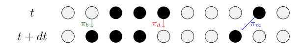
Figure 1: Schematic representation of the time evolution of the system in 1D. Assuming $\sigma_{i}=1$, grey circles represent empty nodes and black circles occupied ones.

Parameter	Meaning
$\Sigma$ (Greek S)	Hypercubic lattice of dimension $d$
$s_{i}$	Number of particles at node $i$
$\sigma_{i}$	Maximum value of $s_{i}$
$N_{i}$ (Greek N)	$\{i\}\cup\{j\in\Sigma\ :\ j$ is a first neighbor of $i\}$
$n_{i}$	Number of particles in $N_{i}$
$\nu_{i}$	Maximum value of $n_{i}$
$P_{i}$ (Greek R)	$\{j\in\Sigma\ :\ |\vec{r}(i)-\vec{r}(j)|\leq R|\}$
$V_{R}$	$2\pi^{d/2}R^{d}/[d\Gamma(d/2)]$, the $d$-volume of $P_{i}$
$m_{i}$	Number of particles in $P_{i}$
$r_{d}$	Rate of death of a particle
$\alpha$	Positive competition parameter
$r_{b}$	Competition-independent part of the particle rate of birth per accessible site
$r_{m}$	Particle rate of jumps per accessible site from node $i$ to $j\in N_{i}$
$c_{1}$	$2dr_{b}/r_{d}$
$c_{2}$	$2d\alpha\rho_{m}V_{R}/r_{d}$
$c_{3}$	$dr_{m}/(N^{2/d}r_{d})$
$c_{4}$	$r_{m}/[2\alpha(NR/L)^{3}]$, parameter used in the 1d case

Table 1: Some parameters and constants used along the work

2.2 Moment equations

From the latter rates, the master equation for the probability $p(S,t)$ of the system being at state $S$ at time $t$ can be written as

$$\frac{\partial}{\partial t}p(S,t)=\sum_{i\in\Sigma} \biggl{\{}(E_{i}^{+}-1)\left[\pi_{d}(s_{i})p(S,t)\right]+(E_{i}^{-}-1)\left[\pi_{b}(s_{i},S)p(S,t)\right]$$ (4)

$$+\sum_{j\in N_{i}-\{i\}}(E_{i}^{+}E_{j}^{-}-1)\left[\pi_{m}(s_{i},s_{j})p(S,t)\right]\biggr{\}},$$

where we have introduced the following operators [32]:

$$E_{i}^{+}f(s_{1},\dots,s_{i},\dots,s_{N})=f(s_{1},\dots,s_{i}+1,\dots,s_{N}),$$ (5)

$$E_{i}^{-}f(s_{1},\dots,s_{i},\dots,s_{N})=f(s_{1},\dots,s_{i}-1,\dots,s_{N}).$$ (6)

The master equation must be solved with any initial normalized and positive $p(S,0)$ verifying

$$p(S,t)=0,\qquad\textrm{if}\quad s_{i}<0\quad\textrm{or}\quad s_{i}>\sigma_{i},$$ (7)

for any $i\in\Sigma$ and $t=0$. Equation (4) guarantees that $p$ is normalized, positive, and condition (7) fulfilled for any $t\geq 0$.

By taking moments of the master equation (4) and using condition (7), we obtain the following equations for the first moments of $p(S,t)$,

$$\frac{d}{dt} \left\langle s_{i}\right\rangle=-r_{d}\left\langle s_{i}\right\rangle+\sum_{j\in N_{i}}\left\langle(r_{b}-\alpha m_{j})_{\theta}s_{j}(\sigma_{i}-s_{i})\right\rangle$$

$$\qquad+r_{m}(\sigma_{i}\left\langle n_{i}\right\rangle-\nu_{i}\left\langle s_{i}\right\rangle),$$

$$\frac{d}{dt} \left\langle s_{i}^{2}\right\rangle=\left\langle\pi_{d}(s_{i})+\pi_{b}(s_{i},S)\right\rangle+\left\langle 2s_{i}\left[\pi_{b}(s_{i},S)-\pi_{d}(s_{i})\right]\right\rangle$$ (9)

$$\qquad+r_{m}\sum_{j\in N_{i}-\{i\}}\left\langle\sigma_{i}s_{j}(1+2s_{i})+\sigma_{j}s_{i}(1-2s_{i})-2s_{i}s_{j}\right\rangle,$$

$$\frac{d}{dt} \left\langle s_{i}s_{j}\right\rangle=-2r_{d}\left\langle s_{i}s_{j}\right\rangle+\left\langle\pi_{b}(s_{i},S)s_{j}+\pi_{b}(s_{j},S)s_{i}\right\rangle$$ (10)

$$\qquad+r_{m}\left[\sigma_{i}\left\langle n_{i}s_{j}\right\rangle+\sigma_{j}\left\langle s_{i}n_{j}\right\rangle-(\nu_{i}+\nu_{j})\left\langle s_{i}s_{j}\right\rangle\right.$$

$$\qquad\qquad\left.-\left(\sigma_{i}\left\langle s_{j}\right\rangle+\sigma_{j}\left\langle s_{i}\right\rangle-2\left\langle s_{i}s_{j}\right\rangle\right)\delta_{i\in N_{j}-\{j\}}\right],\ j\neq i$$

for $i,j\in\Sigma$. We have introduced two new quantities, namely the total number of particles in $N_{i}$:

$$n_{i}\equiv\sum_{j\in N_{i}}s_{j},\\$$ (11)

and its maximum possible value:

$$\nu_{i}\equiv\sum_{j\in N_{i}}\sigma_{j}.$$ (12)

The function $\delta_{i\in A}$ returns $1$ if $i$ belongs to a set $A$ and $0$ otherwise. Each of the three equations (2.2)–(10) contain three terms on their r.h.s. that account the three processes introduced in the model. If we consider Eq. (2.2) as an example, it is apparent that the term proportional to $r_{d}$ (death term) decreases the mean number of particles of node $i$. The second term accounts for the births, with a rate dependent on the occupation of the nearest neighbor sites and of the competition neighborhood $P_{i}$. Finally, the third contribution reflects particle motion.

The system of equations (2.2)–(10), for $i,j\in\Sigma$, is exact but not closed, due to the presence of moments of higher orders. In general, this problem can be circumvented by making the following sequence of approximations: First, we factorize correlations involving $\pi_{b}$:

$$\left\langle\pi_{b}(s_{i},S)f(S)\right\rangle\simeq\sum_{j\in N_{i}}\left\langle(r_{b}-\alpha m_{j})_{\theta}\right\rangle\left\langle s_{j}(\sigma_{i}-s_{i})f(S)\right\rangle,$$

for any function $f(S)$. Second, we also approximate

$$\left\langle(r_{b}-\alpha m_{i})_{\theta}\right\rangle\simeq(r_{b}-\alpha\left\langle m_{i}\right\rangle)_{\theta}.$$ (13)

These two approximations are expected to be correct if $(r_{b}-\alpha m_{i})_{\theta}$ has small fluctuations, which could be the case when $m_{i}$ involves a large number of particles, i.e., when $R$ is big enough, and the mean density of particles is also large. Third, three-node correlations are neglected as

$$\left\langle\left(s_{i}-\left\langle s_{i}\right\rangle\right)\left(s_{j}-\left\langle s_{j}\right\rangle\right)\left(s_{k}-\left\langle s_{k}\right\rangle\right)\right\rangle\simeq 0,$$ (14)

which allows us to express $\left\langle s_{i}s_{j}s_{k}\right\rangle$ as sums of the form $\left\langle s_{i}s_{j}\right\rangle\left\langle s_{k}\right\rangle$. This is a good approximation since the main source of correlations in the model is via particles births, that take place among neighbor node pairs.

It is worth to mention that the latter simplification implies some time limitations to the resulting equations. In particular, if $r_{d}\neq 0$, there is a positive probability for the stochastic particle system to become extinct for any given values of the rest of parameters, implying that $\left\langle s_{i}\right\rangle$ always decays to zero if we wait long enough. In contradiction to that, we anticipate that the simplified equations have stable steady state solutions with $\left\langle s_{i}\right\rangle\neq 0$. Nevertheless we expect, and corroborate with numerical simulations, that the provided simplified description is accurate in a wide time window, useful for understanding relevant observable processes.

With approximations (2.2)–(14), Eqs. (2.2)–(10) become a closed system, but difficult to deal with because of the large number ($N+N^{2}$) of coupled equations. The description can be simplified if we pass to the continuum limit. Two cases will be considered in the next section, namely when there is no restriction on the number of particles at a node (no volume exclusion or $\sigma_{i}\gg 1$) which is the case previously studied in [4], and the novel case of (extreme) volume exclusion where at most one particle can be present in one node.

3 Macroscopic description

3.1 Macroscopic description without volume exclusion

Suppose each node can have a large number of particles, $\sigma_{i}=\sigma\gg 1$ for all $i\in\Sigma$. Then, except for extreme densities, any term of the form $\sigma_{i}-s_{j}$ reduces to $\sigma$. As a consequence, Eqs. in (2.2) with approximations (2.2) and (13), regardless of approximation (14), decouples from the rest, leading to

$$\frac{d}{dt}\left\langle s_{i}\right\rangle=-r_{d}\left\langle s_{i}\right\rangle+\sigma\sum_{j\in N_{i}}(r_{b}-\alpha\left\langle m_{j}\right\rangle)_{\theta}\left\langle s_{j}\right\rangle+r_{m}\sigma\left[\left\langle n_{i}\right\rangle-(2d+1)\left\langle s_{i}\right\rangle\right],\$$ (15)

for $i=1,\dots,N$. Since $\sigma_{i}=\sigma$, we have used the fact that $\nu_{i}=(2d+1)\sigma$.

We now pass to the continuum limit in which the number of nodes $N$ in a system of fixed size $L$ increases, $N\rightarrow\infty$, or equivalently the lattice spacing vanishes $\Delta\equiv L/N^{1/d}\rightarrow 0$. We use the vector position $\vec{r}(i)$ instead of label $i$, $P_{\vec{r}}$ instead of $P_{i}$ (with the same meaning), and the expected value of the density of particles $\rho(\vec{r})$ instead of $\left\langle s_{i}\right\rangle$, with the following identifications

$$i\to\frac{\vec{r}}{\Delta},$$ (16)

$$\left\langle s_{i}\right\rangle\to\frac{\rho(\vec{r},t)}{\rho_{m}},$$ (17)

where

$$\rho_{m}\equiv\frac{N}{L^{d}}=\Delta^{-d}$$ (18)

is the spatial density of lattice nodes. $\sigma\rho_{m}$ is the maximum value allowed to the particle density. For $j\in N_{i}$ we have $|\vec{r}(i)-\vec{r}(j)|=\Delta$, which is much smaller than $L$ for $N\gg 1$. Hence, the continuum limit is a good approximation if $N\gg 1$ for fixed $L$ and $\rho(\vec{r},t)$ is a smooth function of $\vec{r}$, with the following results

$$(r_{b}-\alpha\left\langle m_{j}\right\rangle)_{\theta} \rightarrow \left(r_{b}-\alpha\int_{P_{\vec{r}}}\rho(\vec{r}^{\prime},t)d\vec{r}^{\prime}\right)_{\theta}+\mathcal{O}\left(N^{-1}\right),$$ (19)

$$\left[\left\langle n_{i}\right\rangle-(2d+1)\left\langle s_{i}\right\rangle\right] \rightarrow \frac{L^{2}}{N^{\frac{2}{d}}}\frac{1}{\rho_{m}}\nabla^{2}\rho+\mathcal{O}\left[N^{-\frac{2}{d}-1}\right],$$ (20)

$$\sum_{j\in N_{i}}(r_{b}-\alpha\left\langle m_{j}\right\rangle)_{\theta}\left\langle s_{j}\right\rangle \rightarrow 2d\left(r_{b}-\alpha\int_{P_{\vec{r}}}\rho(\vec{r}^{\prime},t)d\vec{r}^{\prime}\right)_{\theta}\frac{\rho}{\rho_{m}}$$ (21)

$$\qquad+\mathcal{O}\left[N^{-\frac{2}{d}}(\nabla\rho)^{2},N^{-\frac{2}{d}}\nabla^{2}\rho\right].$$

In some limits, for example $r_{m}=0$, the omitted terms in the last expression should be kept in order to account for residual diffusion processes. Finally we arrive at

$$\frac{\partial\rho(\vec{r},t)}{\partial t}= -r_{d}\rho+\sigma\frac{r_{m}}{\rho_{m}^{2/d}}\nabla^{2}\rho+2d\sigma\left[r_{b}-\alpha\int_{P_{\vec{r}}}\rho(\vec{r}~{}^{\prime},t)d\vec{r}~{}^{\prime}\right]_{\theta}\rho,$$ (22)

which is, with an appropriate redefinition of constants, the same non-local Fisher-Kolmogorov equation derived and studied in previous works [4, 33, 34, 35, 36]. In these papers it was justified that the maximum condition for the Heaviside function term was rarely needed so that $\left[r_{b}-\alpha\int_{P_{\vec{r}}}\rho(\vec{r}~{}^{\prime},t)d\vec{r}~{}^{\prime}\right]_{\theta}\approx(r_{b}-\alpha\int_{P_{\vec{r}}}\rho(\vec{r}~{}^{\prime},t)d\vec{r}~{}^{\prime})$ Note that, since $\rho_{m}^{2/d}=\Delta^{-2}$, we recover the usual situation in which a large value of the total jumping rate $\sigma r_{m}$ is needed to keep a nonvanishing diffusion coefficient $\sigma r_{m}\Delta^{2}$ in the continuum limit $N\to\infty$ or $\Delta\to 0$.

3.2 Macroscopic description with volume exclusion

We consider now the situation of full volume exclusion, i.e. at a given time at most one particle can be at a node: $\sigma_{i}=1~{}\forall i\in\Sigma$. In this case the lattice node density $\rho_{m}$ becomes also the maximum possible particle density. We have $\nu_{i}=2d+1$, and $s_{i}(1-s_{i})=0$, or $s_{i}^{2}=s_{i}$, so that Eq. (9) becomes irrelevant. We still have to deal with the system of equations (2.2) and (10).

If we take into account approximations (2.2)–(14), the equation (2.2) for $\left\langle s_{i}\right\rangle$ does not involve terms of the form $\left\langle s_{i}s_{j}\right\rangle$ for $j\notin N_{i}$. As a consequence, in passing to the continuum limit, all we need are the identifications in Eqs. (16) and (17), and one more for terms like $\left\langle s_{i}s_{j}\right\rangle$ for $j\in N_{i}$. In a statistically isotropic system the needed identification should have the form

$$\left\langle s_{i}s_{j}\right\rangle\rightarrow\frac{1}{\rho_{m}^{2}}\kappa(\vec{r},t),\qquad\textrm{for any }j\in N_{i},\textrm{and }i\to\vec{r}/\Delta\ ,$$ (23)

where $\kappa$ is a scalar, rather than a tensor, function. Note that $\kappa$ takes into account the short-range (nearest-neighbor) correlations in the system. The continuum equations, to leading order in $1/N$, reduce to

$$\frac{\partial}{\partial t}\rho(\vec{r},t)=-r_{d}\rho+\frac{r_{m}}{\rho_{m}^{2/d}}\nabla^{2}\rho+$$

$$\qquad 2d\left[r_{b}-\alpha\int_{P_{\vec{r}}}\rho(\vec{r}~{}^{\prime},t)d\vec{r}~{}^{\prime}\right]_{\theta}\left(\rho-\frac{\kappa}{\rho_{m}}\right),$$ (24)

$$\frac{\partial}{\partial t}\kappa(\vec{r},t)=-2r_{d}\kappa-2dr_{m}\left(\kappa-\rho^{2}\right)$$

$$\qquad+2d\left[r_{b}-\alpha\int_{P_{\vec{r}}}\rho(\vec{r}~{}^{\prime},t)d\vec{r}~{}^{\prime}\right]_{\theta}\rho_{m}\rho\left[1+2\left(\frac{\rho}{\rho_{m}}\right)^{2}-3\frac{\kappa}{\rho_{m}^{2}}\right].$$ (25)

System (3.2)–(3.2) can be reduced to a single equation for the density in two interesting cases that we consider in the following.

3.2.1 Correlation factorization at intermediate times.

Suppose first that there are no deaths nor births in the system, $r_{d}=r_{b}=\alpha=0$, so that only the terms containing the jump rate $r_{m}$ remain in Eqs. (3.2)-(3.2). Eq. (3.2) implies that $\kappa$ approaches $\rho^{2}$ in a time of the order of $1/(2dr_{m})$, whereas relaxation times of the density, according to Eq. (3.2), are of the order of $(l/\Delta)^{2}/r_{m}$, with $l$ the typical length of variation of $\rho$. In the continuum description this time is long since $l/\Delta\gg 1$, so that for time scales larger than $1/(2dr_{m})$ we can approximate the time-dependence of $\kappa$ via the density as:

$$\kappa(\vec{r},t)\simeq\left[\rho(\vec{r},t)\right]^{2}.$$ (26)

For general values of the rates $r_{d}$, $r_{b}$ and $\alpha$, Eq. (26) will be still approximately valid for times larger than $1/(2dr_{m})$ provided that $r_{m}$ is large enough so that the corresponding term in Eq. (3.2), describing particle motion, dominates the others. Regardless the relative value of the rates, but if $\rho\simeq\rho_{m}$, the latter approximation also holds, since now almost all nodes are filled. Using Eq. (26) together with Eq. (3.2), we get

$$\frac{\partial}{\partial t}\rho(\vec{r},t)=-r_{d}\rho+\frac{r_{m}}{\rho_{m}^{2/d}}\nabla^{2}\rho+2d\left[r_{b}-\alpha\int_{P_{\vec{r}}}\rho(\vec{r}~{}^{\prime},t)d\vec{r}~{}^{\prime}\right]_{\theta}\left(1-\frac{\rho}{\rho_{m}}\right)\rho.\$$ (27)

This equation can also be derived directly by taking the continuum limit of Eqs. (2.2) and (10), together with approximations (2.2)–(13), and factorizing correlations among all nodes, namely $\left\langle s_{i}s_{j}\right\rangle\simeq\left\langle s_{i}\right\rangle\left\langle s_{j}\right\rangle$ for all $i,j\in\Sigma$ and $i\neq j$.

Equation (27) is the central result of this paper and will be analyzed in detail in the following sections. Two main comments arise about this expression: i) The diffusion constant appearing as the coefficient of the Laplacian term is $r_{m}/\rho_{m}^{2/d}=r_{m}\Delta^{2}$, independent of particle density, as in cases of non-reacting particles with full volume exclusion ($\sigma=1$) [31]. We do not expect this simplicity to remain beyond the $\sigma=1$ and $\sigma=\infty$ limits. ii) The effect of volume exclusion is in the specific form of the birth term (the last one in the r.h.s). Comparing to the no-exclusion case (22) the difference is the additional factor $(1-\rho/\rho_{m})$. It always reduces the birth term and gives a vanishing birth rate when all nodes are occupied. We note that Eq. (27) is different from other non-local cubic equations in the literature [37, 38]. If the range of competitive interaction is much smaller than the typical length-scale variation of $\rho$ (i.e. $R\to 0$), which is the case, for example, when $\rho$ is nearly homogeneous in space, the birth term reduces to $2d(r_{b}-2\alpha V_{R}\rho)(1-\rho/\rho_{m})\rho$ and contains a term proportional to $\rho^{3}$ (where $V_{R}=\int_{P_{\vec{r}}}d\vec{r}^{\prime}=\frac{2\pi^{d/2}}{d\Gamma(d/2)}R^{d}$ is the volume of the $d$-dimensional sphere of radius $R$).

3.2.2 The case of small density.

Another limit in which (3.2)–(3.2) reduces to a single equation for the density corresponds to $\rho\ll\rho_{m}$, i.e. a very dilute system. In this case, it is convenient to expand $\kappa$ in powers of $\rho$, so that at leading order $\kappa\propto\rho$. Keeping only terms linear in the density and taking into account that for $\rho$ small the argument of the $\theta$ function is positive, Eq. (3.2) reduces to

$$\frac{\partial}{\partial t}\kappa(\vec{r},t)=-2r_{d}\kappa-2dr_{m}\kappa+2dr_{b}\rho_{m}\rho.$$ (28)

Once again, when comparing the time-scales of evolution of $\kappa$ in Eq. (28) with the ones for $\rho$ in Eq. (3.2) we conclude that, when the jumping rate $r_{m}$ dominates the other rates, $\kappa$ is related to $\rho$ via the steady–state expression obtained from (28):

$$\kappa(\vec{r},t)\simeq\frac{dr_{b}}{r_{d}+dr_{m}}\rho_{m}\rho(\vec{r},t).$$ (29)

Within this approximation, we get the following equation for the density,

$$\frac{\partial}{\partial t}\rho(\vec{r},t)= -r_{d}\rho+\frac{dr_{m}}{\rho_{m}^{2/d}}\nabla^{2}\rho$$ (30)

$$+2d\left(1-\frac{dr_{b}}{r_{d}+dr_{m}}\right)\left[r_{b}-\alpha\int_{P_{\vec{r}}}\rho(\vec{r}~{}^{\prime},t)d\vec{r}~{}^{\prime}\right]_{\theta}\rho(\vec{r},t).$$

This equation has the same structure as Eq. (22), obtained without volume exclusion, but with different parameters. Here also volume exclusion reduces the effective birth rate. For consistency, since the birth term should be positive, Eq. (30) can only apply if $r_{b}\leq(r_{m}+r_{d}/d)$.

4 Homogeneous solutions and spatial patterns for the excluded-volume birth-death equation

In this section we analyze Eq. (27). As commented before, this is the extension, to include volume exclusion effects, of the already studied spatially non-local birth-death competition model in [4, 33, 34, 35, 36]. This last equation supports homogeneous solutions as well as spatially periodic ones. We analyze here how volume exclusion modifies them. First, it is worth writing Eq. (27) as

$$\frac{\partial}{\partial s}\rho(\vec{r},s) = -\rho+\left[c_{1}-c_{2}\frac{1}{V_{R}\rho_{m}}\int_{P_{\vec{r}}}\rho(\vec{r}^{\prime},s)d\vec{r}^{\prime}\right]_{\theta}\left(1-\frac{\rho}{\rho_{m}}\right)\rho$$ (31)

$$+c_{3}L^{2}\nabla^{2}\rho,$$

where we have defined a new time scale $s=r_{d}t$, and introduced new non–dimensional constants

$$c_{1}\equiv\frac{2dr_{b}}{r_{d}},\qquad c_{2}\equiv\frac{2d\alpha\rho_{m}V_{R}}{r_{d}},\qquad c_{3}\equiv\frac{dr_{m}}{N^{2/d}r_{d}}=\frac{dr_{m}}{r_{d}}(\Delta/L)^{2}.$$ (32)

See a summary of the notation in Table 1. Each constant is proportional to a specific rate measured in units of the death rate: $c_{1}$ is proportional to the birth rate and $c_{3}$ to the rate of movements. $c_{2}$ is proportional to the rate associated to resources competition $\alpha$ and we have also introduced in it the quantity $\rho_{m}V_{R}$ which is the maximum number of particles in a competition neighborhood $P_{\vec{r}}$. This makes more explicit that, if we express all length scales in units of $L$ or of $R$ and write Eq. (32) in terms of $\rho/\rho_{m}\in[0,1]$, the only relevant parameter additional to $c_{1}$, $c_{2}$ and $c_{3}$ is $R/L$. In a large system ($L\to\infty$) the relevant parameters are just $c_{1}$, $c_{2}$ and $c_{3}$. This contrasts with the case without volume exclusion, Eq. (22), which can be written in terms of a single dimensionless parameter for large $L$ [33].

4.1 Homogeneous evolution and steady states

If we focus on spatially homogeneous time-dependent solutions $\rho(x,s)=\rho_{h}(s)$, Eq. (31) reduces to

$$\frac{d\rho_{h}(s)}{ds}=-\rho_{h}(s)+\left[c_{1}-c_{2}\frac{\rho_{h}(s)}{\rho_{m}}\right]_{\theta}\left[1-\frac{\rho_{h}(s)}{\rho_{m}}\right]\rho_{h}(s).$$ (33)

Suppose initially $\rho_{h}(0)\geq\rho_{m}\frac{c_{1}}{c_{2}}$, then the dynamics evolves in two stages:

• For $s\in[0,s_{0}]$ with $s_{0}\equiv\ln\frac{\rho_{h}(0)c_{2}}{\rho_{m}c_{1}}$, we have (note that the term containing the Heaviside function vanishes)

  $$\rho_{h}(s)=\rho_{h}(0)e^{-s}.$$ (34)

• For $s\geq s_{0}$, $\rho_{h}(s)\leq\rho_{m}\frac{c_{1}}{c_{2}}$ and the dynamics becomes more involved. But, since Eq. (33) is an autonomous first-order ordinary differential equation, the only possible behavior is a monotonous approach to one of the available fixed points.

If initially $\rho_{h}(0)\leq\rho_{m}\frac{c_{1}}{c_{2}}$, the dynamics is always at stage (ii). Hence, the system always approaches the steady states within stage (ii).

We can obtain explicit expressions for these steady–state homogeneous solutions $\rho_{h}(\infty)$. They are obtained by equating to zero the r.h.s of Eq. (33), with the following result,

$$\rho_{h}(\infty)=\left\{\begin{array}[]{lcr}\rho_{0}=0&\textrm{ for }&c_{1},c_{2}\geq 0,\\ \rho_{1}=\rho_{m}\left(\frac{c_{1}+c_{2}}{2c_{2}}-\frac{1}{2c_{2}}\sqrt{(c_{1}-c_{2})^{2}+4c_{2}}\right)&\textrm{ for }&c_{1}\geq 1,\ c_{2}\geq 0.\end{array}\right.$$ (35)

For the parameters of the system that make $c_{1}\leq 1$ (we recall that $c_{2}\geq 0$ in this work, since competitive interactions require $\alpha>0$) only the $\rho_{0}$ solution exists, representing complete extinction of the population, while it coexists with another homogeneous solution for $c_{1}>1$. In this last case also a third steady homogeneous solution appears, but it is non-physical since it would give $\rho\geq\rho_{m}$.

4.2 Linear stability analysis of the homogeneous solutions and pattern formation

The stability of the solutions in Eq. (35) can be determined by applying standard linear stability analysis. By adding a perturbation of small amplitude $A$ to the homogeneous states we obtain the linear evolution as

$$\rho(\vec{r},s)=\rho_{h}(\infty)+A\exp\left(\lambda_{\vec{n}}s+i\vec{q}_{\vec{n}}\cdot\vec{r}\right),$$ (36)

where $\vec{q}_{\vec{n}}\equiv\frac{2\pi}{L}\vec{n}$, in terms of the $d$-dimensional vectors of integers $\vec{n}$, are the wavevectors allowed by the periodic boundary conditions.

The specific values of the growth rates $\lambda_{\vec{n}}$ depend on the steady–state solution considered, $\rho_{0}$ or $\rho_{1}$. For the extinction solution, $\rho_{0}=0$, we have

$$\lambda_{\vec{n}}=-\left[1-c_{1}+c_{3}(2\pi\vec{n})^{2}\right].$$ (37)

Since $\lambda_{\vec{n}}\leq\lambda_{\vec{0}}=-(1-c_{1})$, the solution is linearly stable for $c_{1}<1$ and unstable for $c_{1}>1$. In this last case the fastest growth rate occurs for $\vec{n}=\vec{0}$. Therefore we expect the homogeneous solution $\rho_{1}$ to develop after this instability.

When linearizing close to $\rho_{h}(\infty)=\rho_{1}$, the growth rate is

$$\lambda_{\vec{n}}=-\left[\frac{\rho_{1}}{\rho_{m}-\rho_{1}}+c_{3}(2\pi\vec{n})^{2}+c_{2}\frac{\rho_{1}(\rho_{m}-\rho_{1})}{2\rho_{m}^{2}}\mathcal{F}(\vec{q}_{\vec{n}})\right],$$ (38)

where $\mathcal{F}(\vec{q}_{\vec{n}})$ is the Fourier transform of the Heaviside function $\theta(R-|\vec{r}|)$. For large $c_{3}$ (large diffusion) or $c_{2}$ small enough (weak competition or small $R$), and since $\mathcal{F}(\vec{q}_{\vec{n}})$ is a bounded function, $\lambda_{n}$ is negative for all possible $\vec{n}$. On the contrary, if $c_{2}$ becomes large enough, there are values of $\vec{n}$ for which $\lambda_{\vec{n}}$ becomes positive. We expect then that the density will develop periodic patterns with a periodicity given approximately by the wavenumber $\vec{q}_{\vec{n}}$ which first becomes unstable. From generic arguments considering the competition dynamics [35], this periodicity would be in between $R$ and $2R$. The onset of instability is located by solving the following problem

$$\lambda_{\vec{n}}=0,\qquad\vec{\nabla}_{\vec{n}}\lambda_{\vec{n}}=\vec{0}.$$ (39)

Here we solve it explicitly in the one-dimensional case. Now the vectors $\vec{n}$ and $\vec{q}_{\vec{n}}$ become scalars, $n$ and $q_{n}=2\pi n/L$, and the Fourier transform $\mathcal{F}(q_{n})$ is

$$\mathcal{F}(q_{n})=2\frac{\sin(\gamma_{n})}{\gamma_{n}},\qquad\gamma_{n}\equiv q_{n}R=\frac{2\pi R}{L}n,\qquad n=0,\pm 1,\pm 2,...$$ (40)

After some algebra, problem (39) for the onset of instability reduces to

$$c_{4}\left(\gamma_{n}\right)^{2}=\frac{\rho_{1}}{\rho_{m}}\left(1-\frac{\rho_{1}}{\rho_{m}}\right)\left[\frac{\sin\left(\gamma_{n}\right)}{\gamma_{n}}-\cos\left(\gamma_{n}\right)\right],$$ (41)

$$2=c_{2}\left[1-\frac{\rho_{1}}{\rho_{m}}\right]^{2}\left[\cos\left(\gamma_{n}\right)-3\frac{\sin\left(\gamma_{n}\right)}{\gamma_{n}}\right],$$ (42)

where

$$c_{4}\equiv\frac{r_{m}}{2\alpha}\frac{1}{\left(\rho_{m}R\right)^{3}}$$ (43)

is a new parameter that compares the importance of movement with respect to competition. $\rho_{m}R$ is the maximum number of particles in a competition region of size $R$. We recall that the steady-state solution $\rho_{1}/\rho_{m}$ depends also on the constants $c_{1}$ and $c_{2}$ as Eq. (35) shows, hence Eqs. (41) and (42) depend on the parameters of the system through $c_{1}$, $c_{2}$ and $c_{4}$. We can also look at Eqs. (41)–(42) as defining a surface of critical points in the space of parameters $(c_{1},c_{2},c_{4})$, with a critical value of $\gamma_{n}$ assigned to each of these points. From the value of $\gamma_{n}$ one can get the wavenumber $q_{n}$ or $n$, which determine the expected periodicity of the pattern-forming at each instability point as $l\approx 2\pi/q_{n}$. As expected from the explanation of the instability mechanism provided in [35] this periodicity is in between $R$ and $2R$.

The numerical evaluation of Eqs. (41) and (42) for a particular value of $c_{4}$ is shown in Fig. 2 (solid lines). The different regions that we have unveiled, that is, stable zero solution, stable non-zero homogeneous solution, and pattern forming region (corresponding to the instability of $\rho_{1}$) are labelled as R₁, R₂ and R₃, respectively. Note that the transition from the zero solution to the spatial pattern, occurring for a sufficiently large fixed value of $c_{2}$ by increasing $c_{1}$, necessarily passes through the non-zero homogeneous solution (region R₂). But this is not the case numerically observed by simulating the stochastic model (asterisks in the figure) as is discussed in the next section.

Figure 2: Phase diagram indicating three different stability regions (separated by the black lines) from the linear analysis of homogeneous solutions of Eq. (27): in R₁ the vanishing homogeneous state, $\rho_{0}=0$, is stable. In R₂ the non-vanishing homogeneous state $\rho_{1}$ is stable. In R₃ the homogeneous solutions are unstable and periodic patterns would appear. Coefficients $c_{1}$ and $c_{2}$ are defined in (32) while $c_{4}$ is given by (43) and is $c_{4}=5\cdot 10^{-4}$ for the present case. Line with asterisks indicates the transitions obtained from particle simulations where, besides the already stated parameters, $N=2240$ and $R/L=0.1$.

It is worth mentioning that the general formulae of our stability analysis (Eqs. (37) and (38)) are valid in arbitrary dimension and set the qualitative behavior beyond the one-dimensional case on which we focus in this paper. Namely, the phase diagram involves three independent parameters, and the system may exhibit three distinct phases: extinction, spatially homogeneous, and periodic patterns (with dimension-dependent shapes).

5 Numerical simulations of the particle dynamics. Comparison with macroscopic description

In this section we compare the theoretical results of Sec. 4 with numerical simulations, in one dimension and with full volume exclusion ($\sigma=1$), of the stochastic process defined by the rates given in Eqs. (1)-(3). For the parameter values we use $N=2240$, $R/L=0.1$, and $r_{d}=L=1$ (this fixes the units of time and of space, respectively) The quantities $r_{b}$, $\alpha$ and $r_{m}$ (or equivalently $c_{1}$, $c_{2}$ and $c_{3}$, and hence $c_{4}$) have been varied. In the sequel, we explain the algorithm of simulations and then focus on the comparison itself.

5.1 Numerical simulations

We use the Gillespie algorithm [39, 40] to simulate a regular one dimensional system with periodic boundary conditions. An arbitrary initial configuration $S$ of the system is updated in several steps:

• The rates at each node $i=1,\dots N$, associated to the three processes $\pi_{d}(s_{i})$, $\pi_{b}(s_{i},S)$ or $\left[\pi_{m}(s_{i},s_{i-1})+\pi_{m}(s_{i},s_{i+1})\right]$ are calculated, as well as the total rates, given by

  $$\Pi_{d}=\sum_{i=1}^{N}\pi_{d}(s_{i}),$$ (44)

  $$\Pi_{b}=\sum_{i=1}^{N}\pi_{b}(s_{i},S),$$ (45)

  $$\Pi_{m}=\sum_{i=1}^{N}\left[\pi_{m}(s_{i},s_{i-1})+\pi_{m}(s_{i},s_{i+1})\right].$$ (46)

  The current time $t$ is incremented as $t\to t+\Delta t$, where $\Delta t$ is generated with the following exponential density probability

  $$p(\Delta t)=(\Pi_{d}+\Pi_{b}+\Pi_{m})^{-1}\exp\left[(\Pi_{d}+\Pi_{b}+\Pi_{m})\Delta t\right].$$ (47)

• After this time $\Delta t$, one of the three possible events (death, birth or movement) is selected with probability proportional to their corresponding rates ($\Pi_{d}$, $\Pi_{b}$ and $\Pi_{m}$).

• One node, say $i$, is selected with probability proportional to its contribution to the rate of the selected process ($\pi_{d}(s_{i})$, $\pi_{b}(s_{i},S)$ or $\left[\pi_{m}(s_{i},s_{i-1})+\pi_{m}(s_{i},s_{i+1})\right]$).

• Depending on the specific process selected in (ii) and the node involved (iii), the state $S$ of the system is updated: $s_{i}\to 0$ (death), $s_{i}\to 1$ (birth), and $s_{i}\to 0,\ s_{j}\to 1$ (movement), where $j$ is selected equiprobably among the empty next neighbors of $i$.

• If $S$ corresponds to an empty configuration or the desired total time of simulation has been reached, the simulations finishes. In other cases we go back to (i) with the updated state. At some intermediate steps, and under some conditions, properties of interest are measured from the simulations.

5.2 Small birth rates. Decay to the extinction solution

For the region of parameters of the system given by $c_{1}=2r_{b}/r_{d}\leq 1$, the results in Sec. 4 identify extinction as the only homogeneous stable solution of the density equation. We expect then it to be the final outcome also of the particle dynamics. This is confirmed by all numerical simulations run for this region. The left plot of figure 3 shows a typical evolution of the particle system from an initial condition where all nodes are filled (space is plotted in the horizontal axis, and time in the vertical). Particle number decays and they become extinct at long times. When increasing $c_{1}$ the decay process lasts longer and finally, at some critical $c_{1}^{**}$ an absorbing-type phase transition occurs beyond which there is an active phase with a non-vanishing number of particles. On general grounds, and as occurring in the case without excluded volume [41], we expect this transition to be of the directed percolation type. The continuous description leading to the solution $\rho_{1}$ in (35) predicts $c_{1}^{**}=1$, but in the particle system $c_{1}^{**}$ is always larger.

A quantitative comparison with the continuum description requires averaging over multiple realizations to obtain the expected density via $\rho(x,s)=\rho_{m}\left\langle s_{i}\right\rangle$. Additional statistics is gained by further averaging in space to obtain $\bar{\rho}(s)\equiv\int dx\rho(x,s)/L$. Indeed, because of the translational invariance of the system, we expect the average density to be already nearly homogeneous $\rho(x,s)\approx\bar{\rho}(s)$ and then described by the homogeneous dynamics given by Eq. (33). The right panel of Fig. 3 shows the time dependence of $\bar{\rho}$, obtained from the particle simulations. Initially, for high densities such that $\rho/\rho_{m}\geq\frac{c_{1}}{c_{2}}$, dynamics is dominated by deaths and should agree with stage (i) in Sec. 4, so that $\bar{\rho}$ would have an exponential decay with rate $r_{d}$ (or $1$ in units of $r_{d}$, Eq. (34)). Moreover, the larger the birth rate $r_{b}$, keeping the rest of the parameters constant, the smaller the time the system spends in this first stage, in accordance with the estimation of $s_{0}$ just before Eq. (34). For smaller densities a transient would occur within stage (ii), but when $\bar{\rho}$ becomes sufficiently small, the linear dynamics of Eq. (33) or equivalently, Eqs. (36)-(37) with $\vec{n}=\vec{0}$, should take over. Then we expect at long times an exponential decay $\bar{\rho}\sim\exp(-|\lambda|s)$ with exponent $|\lambda|=1-c_{1}$ in units of $r_{d}$ (Eq. (37) for $\vec{n}=\vec{0}$). A third regime, corresponding to the breakdown of the continuum limit (when $\rho/\rho_{m}\sim 1/N$), also appears. It is characterized by the presence of large fluctuations.

Figure 3: Left: spatiotemporal plot of a single realization of the particle dynamics (space in horizontal, time in vertical) for $c_{1}=c_{2}=1,\ c_{4}=5\cdot 10^{-4}$ (region $R_{1}$ of figure 2). The non–dimensional time is $s=r_{d}t$. Right: time dependence of the density (averaged over $100$ realizations) for $c_{2}=1$, $c_{4}=5\cdot 10^{-4}$, and (from bottom to top) $c_{1}=\frac{2}{10},\frac{4}{10},\frac{6}{10},\frac{8}{10},\frac{10}{10}$ (all in region $R_{1}$ of figure 2). Lines are used to indicate different theoretical stages of the dynamics.

Fig. 4 shows (symbols) the decay rates $|\lambda|$ fitted to the exponential decay towards zero of the mean density at long times (but before the large-fluctuation final regime). The two panels represent two different situations. In the left one the mobility $r_{m}$ is larger so that factorization of correlations is justified and the linearization of Eq. (27) (or from (27) or (33)), works well for small $c_{1}$. When increasing $c_{1}$, however, the agreement worsens. We attribute this to the increasing fluctuations occurring when approaching the critical region of the phase transition to the active phase, which occurs at $c_{1}=1$ according to the continuum theory and at a larger value in the particle system. Large critical fluctuations invalidate the assumptions leading to our Eq. (27). For the right panel in Fig. 4, mobility is smaller and nontrivial correlations are apparent at all values of $c_{1}$.

Since in the late stages of density decay $\rho$ is small, it is likely that the approach in Sect. 3.2.2, in which correlations are taken into account approximately in the dilute situation, would work. We linearize Eq. (30) close to $\rho\approx 0$ and plot the resulting decay rate of homogeneous perturbations as a dashed line in the two panels of Fig. 4. We observe some improved agreement, specially in the small mobility (right) case. But still it fails to describe completely the critical region.

Figure 4: Decay rate $|\lambda|$ fitted to the exponential decay towards zero of the mean density at long times, $\bar{\rho}\sim\exp(-|\lambda|s)$, obtained as a function of $c_{1}$ from particle simulations (symbols). Left: $c_{2}=1$, $c_{4}=5\cdot 10^{-4}$. Right: $c_{2}=1$, and $c_{4}=10^{-5}$. Solid lines give the linear prediction from Eq. (27) (or from (27) or (33)), namely $|\lambda|/r_{d}=1-c_{1}$. The dashed lines give the corresponding decay rate from linearization of Eq. (30), which improves the approximation of the correlations in the dilute limit.

5.3 Large birth rates. Homogeneous and non-homogeneous states

For $c_{1}\geq 1$, the theory of section 3.2.1 predicts the existence of non-vanishing homogeneous density solutions, given by Eq. (36). The new solutions have nonzero steady-states values which are stable for $1\leq c_{1}\leq c_{1}^{*}(c_{2},c_{4})$ and unstable for $c_{1}\geq c_{1}^{*}$. In region $c_{1}\geq c_{1}^{*}$ the system would exhibit spatial patterns for long times. For $d=1$, the critical surface $c_{1}^{*}(c_{2},c_{4})$ is given by Eqs. (41)-(42). We see (Fig. 2) that for small $c_{2}$ the system should be homogeneous, and for large $c_{1}$ and $c_{2}$ it should be in a spatially periodic state.

Simulations show partial agreement with these predictions, but also some discrepancies. First, as stated above, the transition from the extinct to the active phase does not occur at $c_{1}=1$, but at $c_{1}=c_{1}^{**}(c_{2},c_{4})>1$ (see asterisks in Fig. 2). For example, for $c_{4}=5\cdot 10^{-4}$, and for both $c_{2}=1$ and $c_{2}=10$, $c_{1}^{**}\simeq 1.5$. This can be understood from a combination of two factors: the stabilization effect of the extinction solution induced by the volume exclusion (via the reduction of the effective birth rate), and the neglected fluctuations and correlations (which are known to stabilize the extinct phase in this type of absorbing transition [33, 41]).

Second, in agreement with the theory, there are periodic (see Fig. 5, left) and homogeneous (not shown) active phases, occurring roughly in the regions predicted, except for the absence of any active phase in the region $1<c_{1}<c_{1}^{*}(c_{2},c_{4})$ (see Fig. 2). The spatial periodicity of the state in the left panel of Fig. 5, is (in units of $L$) approximately $l\approx 1.43R\approx 0.143$, in agreement with the rule $l\in[R,2R]$ which arises from general competitive interaction considerations [35] and from identification of the fastest growing Fourier mode in the linear stability analysis of Sect. 4. This theoretical Fourier mode corresponding to the nearest critical point located at $c_{1}=10$ and $c_{2}\simeq 1.5$ gives $\gamma_{n}^{c}\approx 4.3$ from which the predicted periodicity is $l^{c}\simeq 1.46R$, very close to the observed one. In fact $l\approx 1.43R$ is the periodicity allowed by the periodic boundary conditions closest to $l^{c}$.

Third, the continuum theory predicts that the sequence of steady states encountered when increasing $c_{1}$ at a large-enough value of $c_{2}$, from the zero solution to periodic patterns, includes homogeneous states. The particle simulations do not show this feature, but a direct transition from extinction to inhomogeneous states occurs instead. Whereas the inhomogeneous states develop a clear spatial periodicity when sufficiently far from the transition region (Fig. 5, left), close to the transition line they are more irregular and strongly fluctuating (Fig. 5, right).

Figure 5: Left: Time evolution of a system with $c_{1}=3$, $c_{2}=20$, and $c_{4}=5\cdot 10^{-4}$. Right: evolution of a system with $c_{1}=1.7$, $c_{2}=10$, and $c_{4}=5\cdot 10^{-4}$. The non–dimensional time is $s=r_{d}t$.

We compare in Fig. 6 the mean density $\bar{\rho}$ in the steady state of the particle system with the homogeneous solution $\rho_{1}$ (Eq. (35)) of Eq. (33) for several values of $c_{2}$. For $c_{2}=1$ the particle configurations are statistically homogeneous and then we expect, and observe, reasonable agreement sufficiently far apart from the critical transition region. Fluctuations shift the appearance of the active phase from the deterministic $c_{1}=1$ value to the observed $c_{1}\approx 1.5$. Close to this transition the particle density is smaller than predicted, as usual in similar absorbing-transition situations [33, 41]. For $c_{2}=10$ and $20$ both the particle system and the theoretical description agree in which translational symmetry is broken and inhomogeneous configurations appear. Nevertheless, mean density is quite small, so that coupling of the different modes with the homogeneous one is not strong and still we have that the mean density is well described by the homogeneous prediction: $\bar{\rho}\approx\rho_{1}$.

Figure 6: Steady values of $\bar{\rho}/\rho_{m}$ as a function of $c_{1}$ for $c_{4}=5\cdot 10^{-4}$ and $c_{2}=1$ (circles) and $c_{2}=10$ (triangles). Points correspond to simulations (averaged over $10$ realizations) and lines to the theory.

6 Discussion

We have studied the effects of volume exclusion on a birth-death model with spatially non-local rates. The system models competition since the reproduction rate of any particle decreases if the number of other particles increases in the spatial surroundings. The stochastic model is the basis for macroscopic descriptions and of the simulation results. By taking moments of the master equation of the stochastic model, we encountered an infinite hierarchy of equations. To make the latter description useful, we closed this hierarchy by proposing approximations, some of them beyond the usual correlation factorization approximation and passed to the continuum limit.

Disregarding the volume of the particles we recover previous continuum equations for the density of the system. If the volume of particles is considered, the description changes by the appearance of a new factor in the birth term, $1-\rho/\rho_{m}$. This is given in equation (27) which is a central result of our work. The effect of the new factor is twofold. First, birth rate is always reduced, so that generally the system with volume exclusion will exhibit smaller densities than without it. Second, because of the appearance of two qualitatively new terms in the density equation (27) compared to the case without volume exclusion, Eq. (22), namely the ones proportional to $\rho^{2}$ and to the cubic $\rho^{2}\int\rho~{}dr$, there are two additional dimensionless parameters governing the system behavior, which makes the phase diagram (Fig. 2) richer. In particular regions where the continuum theory predicts homogeneous non-vanishing density is extended towards large $c_{1}$ when $c_{2}$ is small, whereas it only appears for small $c_{1}$ in the absence of volume exclusion [33]. The steady homogeneous solutions of (27) have been fully characterized and the linear and homogeneous nonlinear dynamics towards them discussed. Comparison with the numerical simulations reveals the good agreement of the description for some situations, but at the same time the importance of the correlations when the mobility is small enough (e.g. Fig. 4) and/or near the critical points separating regions $R_{1}$ and $R_{2}$ of figure 2. For bigger values of $r_{m}/r_{d}$, keeping the rest of the parameter constant, the factorization of the correlation as the square of the density becomes a better approximation, and better agreement is obtained. The chosen values of the parameters allowed us to determine the limitations of equation (27).

Linear stability analysis reveals the presence of periodic solutions for large birth and competition, and small mobility. The particle simulations also display these states, although they become rather fluctuating and irregular close to transition points.

The model proposed in this work can be naturally extended along different directions. Regarding the geometry of the underlying lattice, it can be chosen to be a complex network, in general. This would imply direct changes of the different terms appearing on the macroscopic equations. Since the death rate depends on the number of particles and not on the form particles are arranged, its associated terms would not change upon modifying the lattice. Furthermore, at least at the leading order considered in this work where immediate diffusion of particles coming from the birth term is neglected, all geometry dependence of births is encoded in the correlation and the density functions, and hence the influence of the lattice is minimal. Finally, the geometry of the underlining network would be important upon obtaining the result of a diffusion term with position–independent diffusion coefficient, which in the case discussed here of an hypercubic lattice in arbitrary dimension requires only of the restriction on the number of allowed particles per node to be $\sigma=1$ or $\sigma=\infty$. In general, terms that account for movement of particles are different for different lattices. We can go further by allowing the underlying lattice to deform or move in a continuum space, in such a way that it describes now the collective motion of particles like in a crowded environment, extending previous works [42].

We close this discussion by commenting that consideration of volume exclusion opens the door to the study of a large, rather unexplored, field in spatial population dynamics: mutualistic systems. They are characterized by the increase (respectively decrease) of reproduction (death) rates due to the presence of other individuals. Without spatial-dependence most of the models are ill-posed since density grows without limit (see however [43]). In our spatially-dependent case, mutualism would correspond to considering $\alpha$ negative. Due to the excluded volume effect, particle density cannot grow indefinitely. Thus, our model and equations, taken for $\alpha<0$ can be considered to be a well-posed framework to study mutualistic interactions. A detailed study of this case will be presented in future work.

References

References

- [1] Grimm V and Railsback S F, 2005. Individual-Based Modeling and Ecology, Princeton University Press
- [2] Young WR, Roberts AJ, Stuhne G, 2001 Nature 412(6844):328-331
- [3] Zhang Y C, Serva M, and Polikarpov M, 1990 J. Stat. Phys. 58 849
- [4] Hernández-García E and López C, 2004 Phys. Rev. E 70 016216
- [5] Heinsalu E, Hernández-García E, and López C, 2013 Phys. Rev. Lett. 110 258101
- [6] Alder B J and Wainwright T E, 1957 J. Chem. Phys. 27 1208
- [7] Hansen J and McDonald, I R, 2006. Theory of Simple Liquids, Academic Press
- [8] Parisi G and Zamponi F, 2010 Rev. Mod. Phys. 82 789–845
- [9] Khalil N, de Candia A, Fierro A, Ciamarra M P, and Coniglio A, 2014 Soft Matter 10 4800-4805
- [10] Doi M and Edwards S F, 1988. The theory of polymer dynamics (Vol. 73), Oxford University press.
- [11] Marro J and Dickman R, 1999. Nonequilibrium Phase Transitions in Lattice Models, Cambridge University Press
- [12] Krapivsky P L, Mallick K, and Sadhu T, 2014 Phys. Rev. Lett. 113 078101
- [13] Coste C, Delfau J B, Even C, and Saint Jean M, 2010 Phys. Rev. E 81 051201
- [14] Abercrombie M, 1979 Nature 281 259-262
- [15] Maini P K, McElwain D L S, and Leavesley D I, 2004 Tissue Eng. 10 475-482
- [16] Deroulers C, Aubert M, Badoual M, and Grammaticos B, 2009 Phys. Rev. E 79 031917
- [17] Plank M J and Simpson M J, 2012 Journal of The Royal Society Interface 9 76 2983–2996
- [18] Dyson L, Maini P K, and Baker R E 2012 Phys. Rev. E 86 031903
- [19] Grégoire G, Chaté H, and Tu Y, 2001 Phys. Rev. E 64 011902
- [20] Grégoire G and Chaté H, 2004 Phys. Rev. Lett. 92 025702
- [21] Bialké J, Lowen H, and Speck T, 2013 EPL 103 30008
- [22] Elgeti J, and Winkler R G, and Gompper G, 2015 Reports on Progress in Physics 78 (2015)
- [23] Theurkauff I, Cottin-Bizonne C, Palacci J, Ybert C, and Bocquet L, 2012 Phys. Rev. Lett. 108 268303
- [24] Pohl O and Stark H, 2014 Phys. Rev. Lett. 112 238303
- [25] Liebchen B, Marenduzzo D, Pagonabarraga I, and Cates M E, 2015 Phys. Rev. Lett. 115 258301
- [26] Matoz-Fernandez D A, Agoritsas E, Barrat J, Bertin E, Martens E, 2016 arXiv:1611.05282
- [27] Van Beijeren H, Kehr K W, and Kutner R, 1983 Phys. Rev. B 28 5711-5723
- [28] Bruna M, Chapman S J, 2012 Phys. Rev. E 85 011103
- [29] Dyson L, Maini P K , and Baker R E, 2012 Phys. Rev. E 86 031903
- [30] Burger M, Di Francesco M, Pietschmann J F, and Schlake B, 2010 SIAM J. Math. Anal. 42 2842–2871
- [31] Arita C, Krapivsky P L, and Mallick K, 2014 Phys. Rev. E 90 052108
- [32] Van Kampen N G, 1992. Stochastic processes in physics and chemistry, Elsevier
- [33] López C and Hernández-García E, 2004 Physica D 199(1-2): 223-234
- [34] López C and Hernández-García E, 2007 Eur. Phys. J.-ST 146 37-45
- [35] Hernández-García E, Heinsalu E, and López C, 2015 Ecological Complexity 21 166-176
- [36] Fuentes M A, Kuperman M N, and Kenkre V M, 2003 Phys. Rev. Lett. 91 158104
- [37] Clerc M G, Escaff D, and Kenkre V M, 2010 Phys. Rev. E 82 036210
- [38] Escaff D, Fernandez-Oto C, Clerc M G, and Tlidi M, 2015 Phys. Rev. E 91 022924
- [39] Gillespie D T, 1977 J. Phys. Chem. 81 2340
- [40] Heinsalu E, Hernández-García E, López C, 2012 Phys. Rev. E 85 041105
- [41] Lopez C, Ramos F, and Hernandez-Garcia E, 2007 J. Phys. Cond. Matt. 19, 065133
- [42] Bi D, Yang X, Marchetti M C, and Manning M L, 2016 Phys. Rev. X 6 021011
- [43] Holland N J, DeAngelis D L, Bronstein J L, 2002 Am. Nat., 159 231-244