An Efficient Time-splitting Method for the Ehrenfest Dynamics

Abstract

The Ehrenfest dynamics, representing a quantum-classical mean-field type coupling, is a widely used approximation in quantum molecular dynamics. In this paper, we propose a time-splitting method for an Ehrenfest dynamics, in the form of a nonlinearly coupled Schrödinger-Liouville system. We prove that our splitting scheme is stable uniformly with respect to the semiclassical parameter, and, moreover, that it preserves a discrete semiclassical limit. Thus one can accurately compute physical observables using time steps induced only by the classical Liouville equation, i.e., independent of the small semiclassical parameter - in addition to classical mesh sizes for the Liouville equation. Numerical examples illustrate the validity of our meshing strategy.

1 Introduction

Ab initio methods have played a fundamental role in the numerical simulation of large quantum systems, in particular in quantum molecular dynamics. Different from classical approaches based on pre-defined potentials, the underlying idea of ab initio molecular dynamics is to compute the forces acting on the nuclei as a feedback of the electronic structures. This procedure is also known as the “on-the-fly” calculation in the chemistry literature (for detailed reviews, see, e.g., [4, 23, 22, 28]). One of the most widely used of these methods is the so-called Ehrenfest dynamics, a mean-field treatment named in honor of Paul Ehrenfest who was among the first to address the problem of how to derive classical dynamics from the underlying quantum mechanical equations [10]. His idea is to separate the whole system into two parts: a fast varying, quantum mechanical part (for, say, electrons) and a slowly varying part (for the much heavier nuclei) in which one can pass to the (semi-)classical limit. In quantum chemistry, this is usually possible by taking advantage of the large mass difference between electrons and nuclei.

Typically, the Ehrenfest molecular dynamics refers to a Schrödinger equation, coupled with a classical Newtonian flow, cf. [6, 9, 24, 26, 3, 28]. The simplest such model reads

(1.1) $$\left\{\begin{split}ih\partial_{t}\psi&=-\frac{h^{2}}{2}\Delta_{x}\psi+V\left(x,y(t)\right)\psi,\quad\psi(0,x)=\psi_{\rm in}(x),\\ \dot{y}(t)&=\eta(t),\quad y(0)=y_{0},\\ \dot{\eta}(t)&=-\nabla_{y}V_{\rm E}(y(t)),\quad\eta(0)=\eta_{0}.\end{split}\right.$$

Here, we denote by $0<h\ll 1$ a dimensionless rescaled Planck’s constant, and by $\psi=\psi\left(x,t\right)$ with $x\in\mathbb{R}^{d}$, $t\in\mathbb{R}_{+}$, the wave function of the fast, quantum mechanical degrees of freedom, which is assumed to be normalized such that $\|{\psi}(\cdot,t)\|_{L^{2}}=1$ for all $t\geq 0$. In addition, the slow degrees of freedom are described, for any time $t\in\mathbb{R}_{+}$, by their classical position $y(t)\in\mathbb{R}^{n}$ and momentum $\eta(t)\in\mathbb{R}^{n}$. We thereby allow for $n\in\mathbb{N}$ and $d\in\mathbb{N}$ to be not necessarily equal, depending on the physical application. Finally, for a given coupling potential $V=V(x,y)\in\mathbb{R}$, the force describing the back-reaction of the quantum part onto the slow degrees of freedom is given by the gradient in $y\in\mathbb{R}^{n}$ of the so-called Ehrenfest potential

$$V_{\rm E}(y,t)=\int_{\mathbb{R}^{d}}V\left(x,y\right)\left|\psi(x,t)\right|^{2}\,dx.$$

Clearly, one obtains a version of Newton’s second law for $y(t)$ by eliminating the momentum variable $\eta(t)$ and writing

$$\ddot{y}(t)=-\nabla_{y}V_{\rm E}(y(t)),$$

instead of the first order Hamiltonian system above.

Regarding the derivation of Ehrenfest dynamics, the majority of literature available today invokes WKB asymptotics for the slow degrees of freedom, leading to a Hamilton-Jacobi equation which suffers from the appearance of caustics, see, e.g., [6, 24]. To circumvent this problem and derive a semiclassical limit which is valid globally in time, a, by now classical, tool is the Wigner transform [29]. The latter gives rise to a Liouville equation for the associated semi-classical phase-space measure (or, Wigner measure) which “unfolds the caustics”, see [11, 19, 21, 25]. In the context of Ehrenfest dynamics, such an analysis was carried out in [15]. In there, the authors start from a system of time-dependent, self-consistent field equations, motivated by [5, 16, 17, 20], and derive (among other things) the following mixed quantum-classical system:

(1.2) $$\left\{\begin{split}&ih\partial_{t}\psi^{h}=-\frac{h^{2}}{2}\Delta_{x}\psi^{h}+\Upsilon^{h}\left(x,t\right)\psi^{h},\quad\psi^{h}(0,x)=\psi^{h}_{\rm in}(x)\\ &\partial_{t}\mu^{h}+\eta\cdot\nabla_{y}\mu^{h}+F^{h}\left(y,t\right)\cdot\nabla_{\eta}\mu^{h}=0,\quad\mu^{h}(0,x,\eta)=\mu_{\rm in}(y,\eta).\end{split}\right.$$

Here, $\mu^{h}(\cdot,\cdot,t)\in\mathcal{M}^{+}(\mathbb{R}^{n}_{y}\times\mathbb{R}^{n}_{\eta})$ denotes the phase-space probability density for the slowly varying degrees of freedom at time $t$, $F^{h}=-\nabla_{y}V_{\rm E}$, i.e., the force obtained from the Ehrenfest potential, and

(1.3) $$\Upsilon^{h}\left(x,t\right) = \iint_{\mathbb{R}^{2n}}V\left(x,y\right)\mu^{h}\left(y,\eta,t\right)\,dy\,d\eta.$$

We call this system the Schrödinger-Liouville-Ehrenfest (SLE) System and from now on represent the dependence on the small semi-classical parameter $h>0$ by superscripts. Note that the dependence of $\mu^{h}$ on $h$ stems purely from the forcing through the Ehrenfest potential appearing in the Liouville equation. The latter is an Eulerian description of the classical Hamiltonian flow. In particular, one formally obtains (1.1), from (1.2), in the case where $\mu$ corresponds to a single particle distribution concentrated on the classical trajectories $(y(t),\eta(t))$, i.e.,

$$\mu(t,y,\eta)=\delta(y-y(t),\eta-\eta(t)).$$

Such kind of Wigner measures can be obtained as the classical limit of a particular type of wave functions, called semi-classical wave packets, or coherent states, see [19].

Given the dispersive nature of Schrödinger’s equation, the main numerical difficulty for $h\ll 1$ is that one needs to resolve oscillations of frequency of order $\mathcal{O}(1/h)$ in both time and space, as they are present in the solution $\psi^{h}$, see [14] for a broad review of this problem. Naively, this requires one to use time-steps of order $\Delta t=o(h)$ as well as a spatial grid with $\Delta x=o(h)$. However, it was proved in [1], using a Wigner measure analysis, that for a single linear Schrödinger equation, a time-splitting spectral method can still correctly capture physical observables, i.e., real-valued quadratic quantities in $\psi^{h}$, even for time-steps much larger than $h$. Thus one only needs to resolve the high frequency oscillations spatially, which is a huge numerical advantage. For nonlinear Schrödinger equations, in general, this is no longer true, as was numerically demonstrated in [2]. The SLE system (1.2) is a nonlinearly coupled system, and one therefore expects the same type of problem at first glance. Nevertheless, we shall in the following develop an efficient numerical method for the SLE system which allows large (compared with $h$) computational mesh-sizes in both $y$ and $\eta$ and a large time step for both the Schrödinger and the Liouville equations, while still correctly capturing physical observables. While large meshes in $y$ and $\eta$ do not seem so surprising, the possibility of large time steps for solving the Schrödinger equation is far from obvious, due to the nonlinear nature of the SLE system.

Our numerical algorithm is inspired by, but different from the time-splitting method used in [15]. Based on a spectral method for the Schrödinger equation and an upwind scheme for the Liouville part of (1.2), we shall first prove stability for our algorithm, uniformly in $h$. Furthermore, by utilizing the Wigner analysis developed in [15] and adopting it to our particular setting, we shall also prove that physical observables (which can be characterized by the moments of the Wigner distribution), are captured correctly even if $\Delta y$, $\Delta\eta$ and $\Delta t$, i.e., the time step for the entire SLE system, are $\mathcal{O}(1)$ and thus independent of $h$. To this end, we follow the strategy of [1], and prove that the semi-discretized SLE-system, with $\Delta y$, $\Delta\eta$, $\Delta t$ fixed, converges to the correct semiclassical limiting system, as $h\to 0$. In this analysis we shall, for simplicity, consider $x$ to be continuous, since, as already stated above, $\Delta x\to 0$, as $h\to 0$, even for a single linear Schrödinger equation. In summary, our scheme can be seen to be asymptotic-preserving in $t$, $y$, and $\eta$, which is a well-established numerical concept for multi-scale kinetic equations, cf. [12, 13]. To our knowledge, this is the first work that proves the existence of a global in-time $h$-independent meshing strategy for physical observables associated to a nonlinear Schrödinger-type system.

In this context, we note that the authors of [7, 8] study a time-splitting scheme for nonlinear Schrödinger equations with cubic nonlinearity. Using a WKB type representation of the solution, they are able to prove a similar asymptotic preserving property. However, the main drawback of their method is, that it is only valid before the formation of caustics in the Hamilton-Jacobi equation for the WKB phase function. The system studied in the present paper has a weaker nonlinear structure which allows the use of Wigner transformation techniques which are valid for all time $t$.

The rest of this paper is now organized as follows: In Section 2 we present the time-splitting method for the SLE system and briefly discuss some of the inherent numerical difficulties. The stability, uniformly in $h$, is then proved in Section 2.2 for the fully discretized system. In Section 3, we shall give a brief review of Wigner transformation methods and the classical limit of the SLE system. The spatial meshing strategy announced above is then studied in Section 4 by deriving the classical limit of a semi-discrete SLE system. In Section 5 we focus on the time-discretization and prove that our scheme allows for time-steps independent of $h$. Finally, Section 6 presents some numerical examples illustrating our analytical results.

2 The time-splitting scheme and its basic properties

We shall, from now on, consider the Schrödinger-Liouville-Ehrenfest (SLE) System (1.2) with the following assumption on the coupling potential $V$:

(A1) $$V\in C_{0}^{2}\left(\mathbb{R}_{x}^{d}\times\mathbb{R}_{y}^{n}\right)\ \text{and }V\left(x,y\right)\geq 0,\forall\left(x,y\right)\in\mathbb{R}_{x}^{d}\times\mathbb{R}_{y}^{n},$$

where $C^{2}_{0}$ denotes the set of twice continuously differentiable functions which vanish at infinity together with all their derivatives.

Remark 2.1.

This is the same assumption as in [15], where it is used to furnish a rigorous Wigner analysis of the self-consistent field equation. Note that, in particular, it implies $V\in W^{2,\infty}\left(\mathbb{R}_{x}^{d}\times\mathbb{R}_{y}^{n}\right)$. It is conceivable that the regularity requirement and the decay at infinity can be lowered at the expense of more technicalities. The assumption $V(x,y)\geq 0$ is in fact not very restrictive for the potentials bounded from below. It corresponds to a proper choice of the zero point of the potential axis.

We aim for an algorithm which fully utilizes the quantum-classical coupling. Thus, while it makes sense to use a finer (i.e., smaller than $h$) spatial discretization in $x$ to solve the Schrödinger equation, we want to use much larger (than $h$) meshes in $y$ and $\eta$ when solving the Liouville equation. That this is indeed possible is not obvious, since the potential $\Upsilon^{h}\left(x,t\right)$ appearing in the Schrödinger equation is time-dependent, and moreover nonlinearly coupled to the Liouville equation (hence it inherits the computational error obtained from discretizing in $y$ and $\eta$).

Remark 2.2.

In our discussion, we will only consider compactly supported initial data $\psi^{h}_{\rm in}$, $\mu_{\rm in}$, in order to simulate the SLE system problem based on an infinitely large spatial domain within a sufficiently large, but finite box with periodic boundary conditions.

2.1 A new time-splitting scheme for the SLE system

In order to describe our scheme, we henceforth assume that we are given a sufficiently small $\Delta x\sim\mathcal{O}(h)$, used to solve the quantum mechanical part of (1.2), while the larger grid meshes $\Delta y,\Delta\eta\sim\mathcal{O}\left(1\right)$ are applied for the classical part. With this in mind, let

$$J=\frac{d-c}{\Delta y},\ K=\frac{\beta-\alpha}{\Delta\eta},\ M=\frac{b-a}{\Delta x},\ y_{j}=c+j\Delta y,\ \eta_{k}=\alpha+k\Delta\eta,\ x_{j}=a+j\Delta x.$$

The time-splitting spectral scheme can then described as follows: From time $t=t_{n}=n\Delta t$ to $t=t_{n+1}=\left(n+1\right)\Delta t$, with $\Delta t$ given, the SLE system is solved in two steps. First, solve

(2.1) $$\left\{\begin{split}&ih\partial_{t}\psi^{h}=-\frac{h^{2}}{2}\Delta_{x}\psi^{h},\\ &\partial_{t}\mu^{h}=-\eta\cdot\nabla_{y}\mu^{h}-F^{h}\left(y,t\right)\cdot\nabla_{\eta}\mu^{h},\end{split}\right.$$

from $t=t_{n}$ to an intermediate time $t_{\ast}$. Then, solve

(2.2) $$\left\{\begin{split}&ih\partial_{t}\psi^{h}=\Upsilon^{h}\left(x,t\right)\psi^{h},\\ &\partial_{t}\mu^{h}=0,\end{split}\right.$$

with initial data obtained from Step 1, to obtain the solution at time $t=t_{n+1}$.

In (2.1), the Schrödinger equation will be discretized in space by a spectral method and integrated in time exactly using a Fast Fourier Transform. The Liouville equation can be solved either by a spectral method, or by a finite difference (e.g., upwind) scheme in space, and then marching the corresponding ODE system forward in time. An advantage of our splitting method is that in the second step, $\Upsilon^{h}\left(x,t\right)$ defined in (1.3) is indeed independent of time, since obviously $\mu^{h}$ is. In view of this, the time integration in (2.2) can also be solved exactly, which yields

$$\psi_{j}^{h,n+1}=\exp\left(-\frac{i}{h}\Upsilon^{h}\left(x_{j},t_{\ast}\right)\Delta t\right)\psi_{j}^{h,\ast}.$$

For the convenience of our later discussions, we shall now state our numerical scheme using an upwind spatial discretization of $\mu$ in more detail: The problem is solved in one spatial dimension $d=n=1$ from time $t=t_{n}$ to time $t=t_{n+1}$ using the following two steps:

In the first step, we solve

(2.3) $$\left\{\begin{split}&ih\partial_{t}\psi^{h}=-\frac{h^{2}}{2}\partial_{xx}\psi^{h},\\ &\frac{d}{dt}\mu_{jk}^{h}=-\eta_{k}\left(D_{y}\mu^{h}\right)_{jk}-F_{j}^{h}\left(D_{\eta}\mu^{h}\right)_{jk},\end{split}\right.$$

where both $D_{y}\mu^{h}$ and $D_{\eta}\mu^{h}$ represent the numerical derivatives in our algorithm, which are treated using a standard conservative (for example, the upwind type) discretization. To solve the Liouville equation we shall we apply a forward-in-time Euler scheme for the time discretization. Explicitly, we thus have

(2.4) $$\left\{\begin{split}&\psi_{j}^{h,\ast}=\frac{1}{{M}}\sum\limits_{\ell=-{{M}}/2}^{{M}/2-1}e^{-ih\omega_{\ell}^{2}/2}\hat{\psi}_{\ell}^{h,n}e^{i\omega_{\ell}\left(x_{j}-a\right)},\quad j=0,\dots,{M}-1,\\ &\frac{\mu_{jk}^{h,\ast}-\mu_{jk}^{h,n}}{\Delta t}=-\eta_{k}\left(D_{y}\mu^{h,n}\right)_{jk}-F_{j}^{h,n}\left(D_{\eta}\mu^{h,n}\right)_{jk},\end{split}\right.$$

where ${w_{\ell}=\frac{2\pi\ell}{b-1}}$ and, for the upwind spatial discretization,

$$\left\{\begin{split}&\eta_{k}\left(D_{y}\mu^{h,n}\right)_{jk}=\frac{1}{2}\left({\eta_{k}+\left|\eta_{k}\right|}\right)\frac{\mu_{jk}^{h,n}-\mu_{j-1,k}^{h,n}}{\Delta y}+\frac{1}{2}(\eta_{k}-\left|\eta_{k}\right|)\frac{\mu_{j+1,k}^{h,n}-\mu_{j,k}^{h,n}}{\Delta y},\\ &F_{j}^{h,n}\left(D_{\eta}\mu^{h,n}\right)_{jk}=\frac{1}{2}(F_{j}^{h,n}+\left|F_{j}^{h,n}\right|)\frac{\mu_{jk}^{h,n}-\mu_{j,k-1}^{h}}{\Delta\eta}+\frac{1}{2}(F_{j}^{h,n}-\left|F_{j}^{h,n}\right|)\frac{\mu_{j,k+1}^{h,n}-\mu_{jk}^{h,n}}{\Delta\eta}.\end{split}\right.$$

The second step is then given by

(2.5) $$\left\{\begin{split}&ih\partial_{t}\psi^{h}=\Upsilon_{d}^{h}\left(x,t\right)\psi^{h},\\ &\frac{d}{dt}\mu_{jk}^{h}=0,\end{split}\right.$$

where $\Upsilon_{d}^{h}\left(x,t\right)$ is the quadrature approximation of $\Upsilon^{h}\left(x,t\right)$. Thus, we explicitly have

(2.6) $$\begin{split}\psi_{j}^{h,n+1}=\exp\left(-i\Upsilon_{d}^{h,\ast}\left(x_{j}\right){{\Delta t}}/h\right)\psi_{j}^{h,\ast},\quad\mu_{jk}^{h,n+1}=\mu_{jk}^{h,\ast}\end{split}$$

where

$$\Upsilon_{d}^{h,\ast}\left(x\right)=\sum\limits_{j=0}^{J-1}\sum\limits_{k=0}^{K-1}V\left(x,y_{j}\right)\mu_{jk}^{h,\ast}\Delta y\Delta\eta=\sum\limits_{j=0}^{J-1}\sum\limits_{k=0}^{K-1}V\left(x,y_{j}\right)\mu_{jk}^{h,n+1}\Delta y\Delta\eta,$$

which can be viewed as a trapezoidal rule for $\mu$ with compact support, cf. Remark 2.2.

Remark 2.3.

It is straightforward to obtain an algorithm second order in time using the Strang splitting, which is omitted here.

2.2 Conservation property and stability of the scheme

We shall now prove the stability of the scheme given by (2.4) and (2.6). To this end, let $\mathbf{\psi=}\left(\psi_{0},\ldots,\psi_{M-1}\right)^{T}$. Let $\left\|\cdot\right\|_{L^{2}}$ and $\left\|\cdot\right\|_{\ell^{2}}$ be the usual $L^{2}$ and $\ell^{2}$ norm on the interval $\left(a,b\right)$ respectively, i.e.

(2.7) $$\left\|{{\phi}}\right\|_{L^{2}}=\left(\int_{a}^{b}\left|{{\phi}}\left(x\right)\right|^{2}\,dx\right)^{1/2},\quad\left\|\mathbf{\psi}\right\|_{\ell^{2}}=\left(\frac{b-a}{M}\sum\limits_{j=0}^{M-1}\left|\psi_{j}\right|^{2}\right)^{1/2}.$$

Notice that, for any periodic function $f$, the equality

(2.8) $$\left\|f_{\rm I}\right\|^{2}_{L^{2}}=\left\|f\right\|^{2}_{\ell^{2}}=\frac{b-a}{M}\sum\limits_{j=0}^{M-1}\left|f\left(x_{j}\right)\right|^{2}$$

holds, where $f_{\rm I}$ denotes the trigonometric interpolant of $f$ on $\left\{x_{0},x_{1},\ldots,x_{M}\right\}$, i.e.

$$f_{\rm I}\left(x\right)=\frac{1}{M}\sum\limits_{\hat{\jmath}=-\frac{M}{2}}^{\frac{M}{2}-1}\hat{f}_{\hat{\jmath}}e^{i\omega_{\hat{\jmath}}\left(x-a\right)},\quad\omega_{\hat{\jmath}}=\frac{2\pi\hat{\jmath}}{b-a}.$$

Using this we can prove the following theorem.

Theorem 2.4.

The time-splitting spectral scheme conserves the mass. More precisely, it holds

$${\|\mathbf{\psi}^{h,n}\|}_{\ell^{2}}={\|\psi^{h,0}\|}_{\ell^{2}},\quad{\|\psi_{\rm I}^{h,n}\|}_{L^{2}}={\|\psi_{\rm I}^{h,0}\|}_{L^{2}},\quad\text{ for $n=1,2,\dots,$}$$

where, as before, $\psi_{\rm I}^{h,n}$ denotes the trigonometric interpolant of $\psi^{h,n}$. In addition,

$$\sum\limits_{j=0}^{J-1}\sum\limits_{k=0}^{K-1}\mu_{jk}^{h,n}=\sum\limits_{j=0}^{J-1}\sum\limits_{k=0}^{K-1}\mu_{jk}^{h,0}.$$

Proof.

First note that the last identity for $\mu_{jk}^{h,n}$ is a straightforward consequence of the fact that the discretized derivatives $D_{y}\mu$ and $D_{\eta}\mu$ are conservative.

It suffices to prove the first identity stated above due to (2.8). Noting our numerical algorithm (2.4), (2.6) and the definition of the norms (2.7), one computes

$$\frac{1}{b-a}\left\|\mathbf{\psi}^{h,n+1}\right\|_{\ell^{2}}^{2} = \frac{1}{M}\sum\limits_{j=0}^{M-1}\left|\psi_{j}^{h,n+1}\right|^{2}=\frac{1}{M}\sum\limits_{j=0}^{M-1}\left|\exp\left(-\frac{i}{h}\Upsilon_{d}^{h}\left(x_{j},t_{\ast}\right)\Delta t\right)\psi_{j}^{h,\ast}\right|^{2}$$

$$= \frac{1}{M}\sum\limits_{j=0}^{M-1}\left|\psi_{j}^{h,\ast}\right|^{2}=\frac{1}{M}\sum\limits_{j=0}^{M-1}\left|\frac{1}{M}\sum\limits_{\hat{\jmath}=-\frac{M}{2}}^{\frac{M}{2}-1}e^{-ih{{\Delta t}}\omega_{\hat{\jmath}}^{2}/2}\hat{\psi}_{\hat{\jmath}}^{h,n}e^{i\omega_{\hat{\jmath}}\left(x_{j}-a\right)}\right|^{2}$$

$$= \frac{1}{M}\sum\limits_{j=0}^{M-1}\left(\frac{1}{M^{2}}\sum\limits_{p=-\frac{M}{2}}^{\frac{M}{2}-1}\sum\limits_{q=-\frac{M}{2}}^{\frac{M}{2}-1}e^{ih{{\Delta t}}\left(\omega_{p}^{2}-\omega_{q}^{2}\right)/2}\overline{\hat{\psi}_{p}^{h,n}}\hat{\psi}_{q}^{h,n}e^{i\left(\omega_{q}-\omega_{p}\right)\left(x_{j}-a\right)}\right).$$

Changing the order of summation, this is equal to

$$\frac{1}{b-a}\left\|\mathbf{\psi}^{h,n+1}\right\|_{\ell^{2}}^{2} = \frac{1}{M^{2}}\sum\limits_{p=-\frac{M}{2}}^{\frac{M}{2}-1}\sum\limits_{q=-\frac{M}{2}}^{\frac{M}{2}-1}e^{ih{{\Delta t}}\left(\omega_{p}^{2}-\omega_{q}^{2}\right)/2}\overline{\hat{\psi}_{p}^{h,n}}\hat{\psi}_{q}^{h,n}\left(\frac{1}{M}\sum\limits_{j=0}^{M-1}e^{i\left(\omega_{q}-\omega_{p}\right)\left(x_{j}-a\right)}\right)$$

$$= \frac{1}{M^{2}}\sum\limits_{\hat{\jmath}=-\frac{M}{2}}^{\frac{M}{2}-1}\left|\hat{\psi}_{\hat{\jmath}}^{h,n}\right|^{2}=\frac{1}{M^{2}}\sum\limits_{\hat{\jmath}=-\frac{M}{2}}^{\frac{M}{2}-1}\left|\sum\limits_{j=0}^{M-1}\psi_{j}^{h,n}e^{-i\omega_{\hat{\jmath}}\left(x_{j}-a\right)}\right|^{2}$$

$$= \frac{1}{M^{2}}\sum\limits_{\hat{\jmath}=-\frac{M}{2}}^{\frac{M}{2}-1}\left(\sum\limits_{p=0}^{M-1}\sum\limits_{q=0}^{M-1}\overline{\psi_{p}^{h,n}}\psi_{q}^{h,n}e^{i\omega_{\hat{\jmath}}\left(x_{q}-x_{p}\right)}\right),$$

where the second equality of the above follows from the fact that

$$\frac{1}{M}\sum\limits_{j=0}^{M-1}e^{i\left(\omega_{q}-\omega_{p}\right)\left(x_{j}-a\right)}=\frac{1}{M}\sum\limits_{j=0}^{M-1}e^{i2\pi\left(q-p\right)j/M}=\left\{\begin{array}[]{cc}0,&q-p\neq mM\\ 1,&q-p=mM\end{array}\right.,\ m\in\mathbb{Z}.$$

Similarly, by changing the order of summation again, we arrive at

$$\frac{1}{b-a}\left\|\mathbf{\psi}^{h,n+1}\right\|_{\ell^{2}}^{2} = \frac{1}{M}\sum\limits_{p=0}^{M-1}\sum\limits_{q=0}^{M-1}\overline{\psi_{p}^{h,n}}\psi_{q}^{h,n}\left(\frac{1}{M}\sum\limits_{\hat{\jmath}=-\frac{M}{2}}^{\frac{M}{2}-1}e^{i\omega_{\hat{\jmath}}\left(x_{q}-x_{p}\right)}\right)$$

$$= \frac{1}{M}\sum\limits_{j=0}^{M-1}\left|\psi_{j}^{h,n}\right|^{2}=\frac{1}{b-a}\left\|\mathbf{\psi}^{h,n}\right\|_{\ell^{2}}^{2},$$

where the following identity has been used

$$\frac{1}{M}\sum\limits_{\hat{\jmath}=-\frac{M}{2}}^{\frac{M}{2}-1}e^{i\omega_{\hat{\jmath}}\left(x_{q}-x_{p}\right)}=\frac{1}{M}\sum\limits_{\hat{\jmath}=-\frac{M}{2}}^{\frac{M}{2}-1}e^{i2\pi\left(q-p\right)\hat{\jmath}/M}=\left\{\begin{array}[]{cc}0,&q-p\neq mM\\ 1,&q-p=mM\end{array}\right.,\ m\in\mathbb{Z}.$$

∎

Remark 2.5.

Theorem 2.4 implies that the scheme is stable uniformly in $h$, provided the positivity of $\mu$ under the following CFL condition, cf. [18]:

(2.9) $$\max_{k}|\eta_{k}|\frac{\Delta t}{\Delta y}+\left\|\partial_{y}V\right\|_{L^{\infty}}\frac{\Delta t}{\Delta\eta}\leq 1.$$

3 Classical limit of the SLE system

As a preparatory step to the discussion of Section 4, we will now briefly review the results of [15] concerning the classical limit (via Wigner transforms) of the SLE system as $h\to 0$.

3.1 Wigner transform and Wigner measure

Let us first recall that $h$-scaled Wigner transform associated to any continuously parametrized family $f^{h}\equiv\{f^{h}\}_{0\leq h\leq 1}\in L^{2}\left(\mathbb{R}^{d}\right)$ is given by, cf. [11, 19, 21, 25]:

$$w^{h}[f^{h}]\left(x,\xi\right)=\frac{1}{\left(2\pi\right)^{d}}\int_{\mathbb{R}^{d}}f^{h}\left(x-\frac{h}{2}y\right)\overline{f^{h}}\left(x+\frac{h}{2}y\right)e^{i\xi\cdot y}\,dy.$$

By Plancherel’s Theorem and a change of variables one easily finds

$$\left\|w^{h}[f^{h}]\right\|_{L^{2}\left(\mathbb{R}^{2d}\right)}=\frac{1}{\left(2\pi\right)^{\frac{d}{2}}h^{d}}\left\|f^{h}\right\|_{L^{2}\left(\mathbb{R}^{d}\right)}^{2}.$$

The real-valued function $w^{h}(x,\xi)$ acts as a quantum mechanical analogue for classical phase-space distributions. However, $w^{h}(x,\xi)\not\geq 0$ in general.

It has been proved in [19], that if the family of functions $f^{h}=\{f^{h}\}_{0\leq h\leq 1}$ is uniformly bounded in $L^{2}({\mathbb{R}}^{d})$ as $h\to 0_{+}$, i.e., if

$$\sup_{0<h\leq 1}\|f^{h}\|_{L_{x}^{2}}\leq C,$$

then the set of Wigner functions $\{w^{h}\}_{0<h\leq 1}$ is uniformly bounded in $\mathcal{A}^{\prime}$. The latter is the dual of the following Banach space

$$\mathcal{A}({\mathbb{R}}^{d}_{x}\times{\mathbb{R}}^{d}_{\xi}):=\{\chi\in C_{0}({\mathbb{R}}^{d}_{x}\times{\mathbb{R}}^{d}_{\xi})\,:\,(\mathcal{F}_{\xi}\chi)(x,z)\in L^{1}({\mathbb{R}}^{d}_{z};C_{0}({\mathbb{R}}^{d}_{x}))\},$$

where $C_{0}({\mathbb{R}}^{d})$ denotes the space of continuous functions vanishing at infinity and $\mathcal{F}_{\xi}$ denotes the Fourier transform with respect to the velocity $\xi$, only. More precisely, one finds that for any test function $\chi\in\mathcal{A}({\mathbb{R}}^{d}_{x}\times{\mathbb{R}}^{d}_{\xi})$,

$$|\langle w^{h},\chi\rangle|\leq\frac{1}{(2\pi)^{d}}{\|\chi\|}_{\mathcal{A}}{\|f^{h}\|}^{2}_{L^{2}}\leq{\rm const.},$$

uniformly in $h$. Thus, up to extraction of sub-sequences $\{h_{n}\}_{n\in{\mathbb{N}}}$, with $h_{n}\to 0_{+}$ as $n\to\infty$, there exists a limiting object $w^{0}\equiv w\in\mathcal{A}^{\prime}({\mathbb{R}}^{d}_{x}\times{\mathbb{R}}^{d}_{\xi})$ such that

$$w^{h}\stackrel{{\scriptstyle h\rightarrow 0_{+}}}{{\longrightarrow}}w\quad\text{in $\mathcal{A}^{\prime}({\mathbb{R}}^{d}_{x}\times{\mathbb{R}}^{d}_{\xi}){\rm w-\ast}$}.$$

It turns out that the limit is in fact a non-negative, bounded Borel measure on phase-space $w\in\mathcal{M}^{+}({\mathbb{R}}^{d}_{x}\times{\mathbb{R}}^{d}_{p})$, called the Wigner measure of $f^{h}$.

3.2 The Classical limit of the SLE system

Let $\psi^{h}$ and $\mu^{h}$ be the solution of the SLE system (1.2) and denote the Wigner function of $\psi^{h}\left(x,t\right)$ by

$$w^{h}\left(x,\xi,t\right)=w^{h}[\psi^{h}\left(\cdot,t\right)]\left(x,\xi\right).$$

A straightforward computation shows that the position density associated to $\psi^{h}\in L^{2}({\mathbb{R}}^{d})$ can be computed via

$${{\rho}}^{h}\left(x,t\right):=\left|\psi^{h}\left(x,t\right)\right|^{2}=\int_{\mathbb{R}^{d}}w^{h}\left(x,\xi,t\right)d\xi,$$

where we recall, that due to our normalization,

$$\int_{{\mathbb{R}}^{d}}{{\rho}}^{h}\left(x,t\right)\,dx=\iint_{\mathbb{R}^{2d}}w^{h}\left(x,\xi,t\right)d\xi\,dx=1.$$

Moreover, by taking higher order moments in $\xi$ one (formally) finds the current density

$$j^{h}\left(x,t\right):=h\mathop{\rm Im}\left(\overline{\psi^{h}\left(x,t\right)}\nabla\psi^{h}\left(x,t\right)\right)=\int_{\mathbb{R}^{d}}\xi w^{h}\left(x,\xi,t\right)d\xi,$$

and the kinetic energy density

$$\kappa^{h}\left(x,t\right):=\frac{h^{2}}{2}\left|\nabla\psi^{h}\left(x,t\right)\right|^{2}=\int_{\mathbb{R}^{d}}\frac{1}{2}\left|\xi\right|^{2}w^{h}\left(x,\xi,t\right)d\xi.$$

Remark 3.1.

In order to make these computations rigorous, the integrals on the r.h.s. have to be understood in an appropriate sense, since $w^{h}\not\in L^{1}({\mathbb{R}}^{m}_{x}\times{\mathbb{R}}^{m}_{\xi})$ in general, see [19] for more details.

After Wigner transforming the Schrödinger equation, one finds that $w^{h}\left(x,\xi,t\right)$ satisfies the following nonlocal kinetic equation (see, e.g., [19]):

$$\partial_{t}w^{h}+\xi\cdot\nabla_{x}w^{h}+\Theta^{h}[\Upsilon^{h}]w^{h}=0,\quad w^{h}(0,x,\xi)=w_{\rm in}^{h}\left(x,\xi\right),$$

where $w_{\rm in}^{h}\equiv w^{h}[\psi^{h}_{\rm in}]$ and

(3.1) $$\left(\Theta^{h}[\Upsilon^{h}]w^{h}\right)\left(x,\xi,t\right)=\frac{i}{h(2\pi)^{d}}\int_{\mathbb{R}^{d}}\left(\Upsilon^{h}\left(x+\frac{h}{2}z,t\right)-\Upsilon^{h}\left(x-\frac{h}{2}z,t\right)\right)\widehat{w}^{h}(x,z,t)e^{iz\cdot\xi}dz$$

with $\widehat{w}^{h}$ denoting the Fourier transformation of $w^{h}$ w.r.t. the second variable only.

Now, in order to utilize the weak-$\ast$ compactness properties of the Wigner function, we shall impose from now on that the initial mass and the initial kinetic energy are uniformly bounded with respect to $h$, i.e.,

(A2) $$\sup\limits_{0<h\leq 1}\left({{\rho}}^{h}\left(x,0\right)+\kappa^{h}\left(x,0\right)\right)\leq\text{const.}$$

Remark 3.2.

In other words, we assume that

$$\sup\limits_{0<h\leq 1}\left(\left|\psi_{\rm in}^{h}(x)\right|^{2}+\frac{h^{2}}{2}\left|\nabla\psi_{\rm in}^{h}(x)\right|^{2}\right)\leq\text{const.}$$

This assumption is easily satisfied by initial data of WKB type, or by semi-classical wave packets.

It is proved in [15] that these uniform bounds on the initial mass and kinetic energy are propagated by the SLE system (1.2), which in turn implies that for all times $t\in{\mathbb{R}}_{+}$, the wave function $\psi^{h}(\cdot,t)$ is:

1. uniformly bounded in $L^{2}\left(\mathbb{R}^{d}\right)$ as $h\rightarrow 0^{+}$, i.e.

   $$\underset{0<h\leq 1}{\sup}\left\|\psi^{h}(\cdot,t)\right\|_{L_{x}^{2}}\leq C_{1},$$

2. $h$-oscillatory, i.e.

   $$\underset{0<h\leq 1}{\sup}\left\|h\nabla_{x}\psi^{h}(\cdot,t)\right\|_{L_{x}^{2}}\leq C_{2},$$

   where $C_{1}$ and $C_{2}$ are some constants independent of $0<h<1$.

In particular this implies the existence of a limiting Wigner measure $\nu(\cdot,\cdot,t)\in\mathcal{M}^{+}(\mathbb{R}_{x}^{d}\times\mathbb{R}_{\xi}^{d})$, such that for all $T>0$

$$w^{h}\left[\psi^{h}\right]\stackrel{{\scriptstyle h\rightarrow 0_{+}}}{{\longrightarrow}}\nu\ \ \text{in }L^{\infty}([0,T];\mathcal{A}^{\prime}\left(\mathbb{R}_{x}^{d}\times\mathbb{R}_{\xi}^{d})\right)\text{w--}\ast,$$

up to the extraction of subsequences. Moreover, on the same time-interval, one has

$$\left|\psi^{h}(x,t)\right|^{2}\stackrel{{\scriptstyle h\rightarrow 0_{+}}}{{\longrightarrow}}\int_{\mathbb{R^{d}}}\nu\left(x,\xi,t\right)d\xi\ \text{in }\mathcal{M}^{+}\left(\mathbb{R}^{d}_{x}\right)\text{w--}\ast.$$

Under our assumption (A1) on $V$, this can be used to prove that (see [15] for more details):

$$F^{h}\left(y,t\right)\stackrel{{\scriptstyle h\rightarrow 0_{+}}}{{\longrightarrow}}-\iint_{{\mathbb{R}}^{2d}}\nabla_{y}V\left(x,y\right)\nu(x,\xi,t)\,dx\,d\xi=:F^{0}\left(y,t\right),$$

uniformly on compact intervals in $y$ and $t$.

Similarly, one can pass to the limit $h\to 0_{+}$ in the equation for $\mu^{h}$ to find that there exists a limiting measure $\mu^{0}\equiv\mu\in\mathcal{M}^{+}({\mathbb{R}}^{n}_{y}\times{\mathbb{R}}^{n}_{\eta})$ which consequently solves (in the sense of distributions):

(3.2) $$\partial_{t}\mu+\eta\cdot\nabla_{y}\mu+F^{0}\left(y,t\right)\cdot\nabla_{\eta}\mu=0.$$

Moreover, one can prove that

$$\Upsilon^{h}\left(x,t\right)\stackrel{{\scriptstyle h\rightarrow 0_{+}}}{{\longrightarrow}}\iint_{\mathbb{R}^{2n}}V\left(x,y\right)\mu\left(y,\eta,t\right)\,dy\,d\eta=:\Upsilon^{0}\left(x,t\right).$$

In view of the definition (3.1), one also finds that

$$\Theta^{h}\left[\Upsilon^{h}\right]w^{h}\stackrel{{\scriptstyle h\rightarrow 0_{+}}}{{\longrightarrow}}-\nabla_{x}\Upsilon^{0}\left(x,t\right)\cdot\nabla_{\xi}\nu$$

and thus, the Wigner measure associated to $\psi^{h}$ satisfies the following Liouville equation (in the sense of distributions):

(3.3) $$\partial_{t}\nu+\xi\cdot\nabla_{x}\nu-\nabla_{x}\Upsilon^{0}\left(x,t\right)\cdot\nabla_{\xi}\nu=0.$$

In summary, one finds a system of two coupled Liouville equations (3.2)–(3.3) in the classical limit (we refer to [15] for a rigorous proof and further details).

4 The spatial meshing strategy

4.1 The semi-discretized SLE system and its energy

The analysis in this section will focus on the spatial meshing strategy. In order to show that it is possible to use a grid with $\Delta y,\Delta\eta\sim O(1)$, and thus, independent of $h$, we will consider a semi-discretized version of the SLE system (1.2) in one spatial dimension $d=n=1$ where the Liouville is discretized using an upwind scheme:

(4.1) $$\left\{\begin{split}&ih\partial_{t}\psi^{h}=-\frac{h^{2}}{2}\partial_{xx}\psi^{h}+\Upsilon_{d}^{h}\left(x,t\right)\psi^{h},\quad\psi^{h}(0,x)=\psi_{\rm in}^{h}(x),\\ &\partial_{t}\mu^{h}+\eta D_{y}\mu^{h}+F^{h}\left(y,t\right)D_{\eta}\mu^{h}=0,\quad\mu^{h}(0,y,\eta)=\mu_{\rm in}^{h}(y,\eta).\end{split}\right.$$

Here, $\Upsilon_{d}^{h}\left(x,t\right)$ stands for the trapezoidal quadrature approximation of $\Upsilon^{h}\left(x,t\right)$, as before, whereas $F^{h}\left(y,t\right)$ includes exact derivative of the known function $V\left(x,y\right)$. We shall refer to (4.1) as the semi-discretized SLE system (s-SLE) and show that it yields the “correct” classical limit, i.e., the semi-discretized version of (3.2)–(3.3).

Before doing so, we will need to prove an a-priori estimate and the energy associated to (4.1). To this end, we define the semi-discrete energy as

$$E_{d}\left(t\right):=\int_{\mathbb{R}}\frac{h^{2}}{2}\left|\partial_{x}\psi^{h}(x,t)\right|^{2}dx+\int_{\mathbb{R}}\Upsilon_{d}^{h}\left(x,t\right)\left|\psi^{h}\right|^{2}dx+\sum\limits_{j=0}^{J-1}\sum\limits_{k=0}^{K-1}\frac{\eta_{k}^{2}}{2}\mu_{jk}^{h}\Delta y\Delta\eta.$$

Here, and in the following, because of the periodicity of $\mu$, we shall use a cyclic index for $\mu_{jk}$, such that $\mu_{jk}=\mu_{j+J,k}=\mu_{j-J,k}=\mu_{j,k+K}=\mu_{j,k-K}$.

Theorem 4.1.

Under the assumptions (A1) and (A2), the energy $E_{d}(t)$ is bounded by a constant independent of $h$ for all $t\geq 0$.

Proof.

We start by showing that the initial energy is bounded. This is easily seen from

$$E_{d}\left(0\right)=\int_{\mathbb{R}}\frac{h^{2}}{2}\left|\partial_{x}\psi_{\rm in}^{h}\right|^{2}dx+\int_{\mathbb{R}}\Upsilon_{d}^{h}\left(x,0\right)\left|\psi_{\rm in}^{h}\right|^{2}dx+\sum\limits_{j=0}^{J-1}\sum\limits_{k=0}^{K-1}\left(\mu_{\rm in}\right)_{jk}\Delta y\Delta\eta,$$

where the first two integrals are clearly bounded by assumptions (A1) and (A2) and the last term is just a quadrature approximation of $\iint\mu_{\rm in}\,dy\,d\eta=1$, and hence bounded.

Next, we compute the time-derivative of $E_{d}$ as

$$\frac{d}{dt}E_{d}=(\text{I})+(\text{II})+(\text{III})+\text{(IV),}\ \$$

where

$$(\text{I}) := \int_{\mathbb{R}}\frac{h^{2}}{2}\left(\partial_{x}\partial_{t}\bar{\psi}^{h}\cdot\partial_{x}\psi^{h}+\partial_{x}\bar{\psi}^{h}\cdot\partial_{x}\partial_{t}\psi^{h}\right)dx,$$

$$(\text{II}) := \int_{\mathbb{R}}\Upsilon_{d}^{h}\left(x,t\right)\left(\partial_{t}\bar{\psi}^{h}\psi^{h}+\bar{\psi}^{h}\partial_{t}\psi^{h}\right)dx,$$

$$(\text{III}) := \int_{\mathbb{R}}\partial_{t}\Upsilon_{d}^{h}\left(x,t\right)\left|\psi^{h}\right|^{2}dx,$$

$$(\text{IV}) := \sum\limits_{j=0}^{J-1}\sum\limits_{k=0}^{K-1}\frac{\eta_{k}^{2}}{2}\left(\partial_{t}\mu^{h}\right)_{jk}\Delta y\Delta\eta.$$

First, a straightforward calculation shows $($I$)+($II$)=0$, since

$$(\text{I})+(\text{II}) = -\int_{\mathbb{R}}\frac{h^{2}}{2}\left(\partial_{t}\bar{\psi}^{h}\partial_{xx}\psi^{h}+\partial_{xx}\bar{\psi}^{h}\partial_{t}\psi^{h}\right)dx+\int_{\mathbb{R}}\Upsilon_{d}^{h}\left(\partial_{t}\bar{\psi}^{h}\psi^{h}+\bar{\psi}^{h}\partial_{t}\psi^{h}\right)dx$$

$$= \int_{\mathbb{R}}\partial_{t}\bar{\psi}^{h}\left(-\frac{h^{2}}{2}\partial_{xx}\psi^{h}+\Upsilon_{d}^{h}\psi^{h}\right)+\left(-\frac{h^{2}}{2}\partial_{xx}\bar{\psi}^{h}+\Upsilon_{d}^{h}\bar{\psi}^{h}\right)\partial_{t}\psi^{h}dx$$

$$= \int_{\mathbb{R}}\partial_{t}\bar{\psi}^{h}\left(ih\partial_{t}\psi^{h}\right)+\left(-ih\partial_{t}\bar{\psi}^{h}\right)\partial_{t}\psi^{h}dx=0.$$

For simplicity we will, from now on, denote

$$G_{j}^{h}(t)\equiv G^{h}\left(t,x,y_{j}\right)=\int_{\mathbb{R}}V\left(x,y_{j}\right)\left|\psi^{h}(t,x)\right|^{2}\,dx\geq 0,$$

as well as

$$F_{j}^{h}(t)\equiv F^{h}\left(y_{j},t\right)=-\int_{\mathbb{R}}\partial_{y}V\left(x,y_{j}\right)\left|\psi^{h}\right|^{2}dx.$$

A key observation is that $G^{h}$ is in fact Lipschitz with a Lipschitz constant $L>0$ independent of $h$, since

$$\left|G_{j+1}^{h}-G_{j}^{h}\right|=\left|\int_{\mathbb{R}}\left[V\left(x,y_{j+1}\right)-V\left(x,y_{j}\right)\right]\left|\psi^{h}\right|^{2}dx\right|\leq\int_{\mathbb{R}}\left|\partial_{y}V\left(x,\xi\right)\right|\left|y_{j+1}-y_{j}\right|\left|\psi^{h}\right|^{2}dx,$$

for some $\xi\in\left(y_{j},y_{j+1}\right)$. Thus

$$\left|G_{j+1}^{h}-G_{j}^{h}\right|\leq\left\|\partial_{y}V\left(x,\xi\right)\right\|_{L^{\infty}}\left\|\psi^{h}\right\|_{L^{2}}^{2}\left|y_{j+1}-y_{j}\right|=\left\|\partial_{y}V\left(x,\xi\right)\right\|_{L^{\infty}}\Delta y=:L\Delta y,$$

since $\left\|\psi^{h}\right\|_{L^{2}}=\left\|\psi_{\rm in}^{h}\right\|_{L^{2}}=1$, in view of mass conservation established in Theorem 2.4. In addition, we have that $F^{h}_{j}$ is uniformly bounded, i.e.

(4.2) $$\left|F_{j}^{h}\right|=\left|\int_{\mathbb{R}}\partial_{y}V\left(x,y_{j}\right)\left|\psi^{h}\right|^{2}dx\right|\leq\left\|\partial_{y}V\left(x,\xi\right)\right\|_{L^{\infty}}\left\|\psi^{h}\right\|_{L^{2}}^{2}=L.$$

Coming back to $($III$)$, we first note

$$\partial_{t}\Upsilon_{d}^{h}\left(x,t\right) = \sum\limits_{j=0}^{J-1}\sum\limits_{k=0}^{K-1}V\left(x,y_{j}\right)\left(\partial_{t}\mu^{h}\right)_{jk}\Delta y\Delta\eta$$

$$= -\sum\limits_{j=0}^{J-1}\sum\limits_{k=0}^{K-1}V\left(x,y_{j}\right)\left[\eta_{k}\left(D_{y}\mu^{h}\right)_{jk}+F_{j}^{h}\left(D_{\eta}\mu^{h}\right)_{jk}\right]\Delta y\Delta\eta$$

$$= -\sum\limits_{j=0}^{J-1}\sum\limits_{k=0}^{K-1}V\left(x,y_{j}\right)\eta_{k}\left(D_{y}\mu^{h}\right)_{jk}\Delta y\Delta\eta,$$

where the last equality follows from the fact that we have a telescoping series in $k$ with zero boundary conditions. Recalling (4.1), $($III$)$ can be written as

$$(\text{III}) = -\sum\limits_{j=0}^{J-1}\sum\limits_{k=0}^{K-1}G_{j}^{h}\eta_{k}\left(D_{y}\mu^{h}\right)_{jk}\Delta y\Delta\eta$$

$$= -\sum\limits_{j=0}^{J-1}\sum\limits_{k=0}^{K-1}G_{j}^{h}\frac{\eta_{k}+\left|\eta_{k}\right|}{2}\left(\mu_{jk}^{h}-\mu_{j-1,k}^{h}\right)\Delta\eta-\sum\limits_{j=0}^{J-1}\sum\limits_{k=0}^{K-1}G_{j}^{h}\frac{\eta_{k}-\left|\eta_{k}\right|}{2}\left(\mu_{j+1,k}^{h}-\mu_{j,k}^{h}\right)\Delta\eta$$

$$= \sum\limits_{j=0}^{J-1}\sum\limits_{k=0}^{K-1}\frac{\eta_{k}+\left|\eta_{k}\right|}{2}\mu_{jk}^{h}\left(G_{j+1}^{h}-G_{j}^{h}\right)\Delta\eta+\sum\limits_{j=0}^{J-1}\sum\limits_{k=0}^{K-1}\frac{\left|\eta_{k}\right|-\eta_{k}}{2}\mu_{jk}^{h}\left(G_{j-1}^{h}-G_{j}^{h}\right)\Delta\eta,$$

where summation by parts is used in the last equality. In view of the Lipschitz property above, it is then straightforward to estimate $($III$)$ via

$$(\text{III})\leq L\sum\limits_{j=0}^{J-1}\sum\limits_{k=0}^{K-1}\left|\eta_{k}\right|\mu_{jk}^{h}\Delta y\Delta\eta.$$

Similarly, one proves that

$$(\text{IV}) = -\sum\limits_{j=0}^{J-1}\sum\limits_{k=0}^{K-1}\frac{\eta_{k}^{2}}{2}F_{j}^{h}\left(D_{\eta}\mu^{h}\right)_{jk}\Delta y\Delta\eta$$

$$= -\sum\limits_{j=0}^{J-1}\sum\limits_{k=0}^{K-1}\frac{\eta_{k}^{2}}{2}\frac{F_{j}^{h}+\left|F_{j}^{h}\right|}{2}\left(\mu_{jk}^{h}-\mu_{j,k-1}^{h}\right)\Delta y-\sum\limits_{j=0}^{J-1}\sum\limits_{k=0}^{K-1}\frac{\eta_{k}^{2}}{2}\frac{F_{j}^{h}-\left|F_{j}^{h}\right|}{2}\left(\mu_{j,k+1}^{h}-\mu_{jk}^{h}\right)\Delta y$$

$$= \sum\limits_{j=0}^{J-1}\sum\limits_{k=0}^{K-1}\frac{\eta_{k+1}^{2}-\eta_{k}^{2}}{2}\frac{F_{j}^{h}+\left|F_{j}^{h}\right|}{2}\mu_{jk}^{h}\Delta y+\sum\limits_{j=0}^{J-1}\sum\limits_{k=0}^{K-1}\frac{\eta_{k}^{2}-\eta_{k-1}^{2}}{2}\frac{F_{j}^{h}-\left|F_{j}^{h}\right|}{2}\mu_{jk}^{h}\Delta y$$

$$= \sum\limits_{j=0}^{J-1}\sum\limits_{k=0}^{K-1}\left(\eta_{k}+\frac{\Delta\eta}{2}\right)\Delta\eta\frac{F_{j}^{h}+\left|F_{j}^{h}\right|}{2}\mu_{jk}^{h}\Delta y+\sum\limits_{j=0}^{J-1}\sum\limits_{k=0}^{K-1}\left(\eta_{k}-\frac{\Delta\eta}{2}\right)\Delta\eta\frac{F_{j}^{h}-\left|F_{j}^{h}\right|}{2}\mu_{jk}^{h}\Delta y,$$

where summation by parts is used as before. Combining the coefficients of $F_{j}^{h}$ and $\left|F_{j}^{h}\right|$ respectively, this is equal to

$$(\text{IV}) = \sum\limits_{j=0}^{J-1}\sum\limits_{k=0}^{K-1}\eta_{k}F_{j}^{h}\mu_{jk}^{h}\Delta y\Delta\eta+\sum\limits_{j=0}^{J-1}\sum\limits_{k=0}^{K-1}\frac{\Delta\eta}{2}\left|F_{j}^{h}\right|\mu_{jk}^{h}\Delta y\Delta\eta$$

$$\leq L\sum\limits_{j=0}^{J-1}\sum\limits_{k=0}^{K-1}\left|\eta_{k}\right|\mu_{jk}^{h}\Delta y\Delta\eta+L\sum\limits_{j=0}^{J-1}\sum\limits_{k=0}^{K-1}\frac{\Delta\eta}{2}\mu_{jk}^{h}\Delta y\Delta\eta.$$

In summary, we thus find

$$\frac{d}{dt}E_{d}\leq 2L\sum\limits_{j=0}^{J-1}\sum\limits_{k=0}^{K-1}\left|\eta_{k}\right|\mu_{jk}^{h}\Delta y\Delta\eta+L\sum\limits_{j=0}^{J-1}\sum\limits_{k=0}^{K-1}\frac{\Delta\eta}{2}\mu_{jk}^{h}\Delta y\Delta\eta$$

$$\leq 2L\left(\sum\limits_{j=0}^{J-1}\sum\limits_{k=0}^{K-1}\eta_{k}^{2}\mu_{jk}^{h}\Delta y\Delta\eta\right)^{\frac{1}{2}}\left(\sum\limits_{j=0}^{J-1}\sum\limits_{k=0}^{K-1}\mu_{jk}^{h}\Delta y\Delta\eta\right)^{\frac{1}{2}}+L\sum\limits_{j=0}^{J-1}\sum\limits_{k=0}^{K-1}\frac{\Delta\eta}{2}\mu_{jk}^{h}\Delta y\Delta\eta.$$

Using the fact that

$$\sum\limits_{j=0}^{J-1}\sum\limits_{k=0}^{K-1}\mu_{jk}^{h}\Delta y\Delta\eta=C$$

is a conserved quantity with respect to time, we consequently find the following estimate

$$\frac{d}{dt}E_{d}\left(t\right) \leq 2^{\frac{3}{2}}LC^{\frac{1}{2}}\sqrt{E_{d}\left(t\right)}+\frac{LC}{2}\Delta\eta$$

$$\leq E_{d}\left(t\right)+2L^{2}C+\frac{LC}{2}\Delta\eta\equiv E_{d}\left(t\right)+C_{1}.$$

By Gronwall’s inequality, this yields

$$E_{d}\left(t\right)\leq\left(C_{1}+E_{d}(0)\right)e^{t}-C_{1}\text{,}$$

which gives the desired bound independent of $h$. ∎

Remark 4.2.

It is easy to find a sharper bound of the energy by considering times $t\leq e$ and $t>e$, respectively, but the estimate above is sufficient for our purposes.

4.2 The classical limit of the s-SLE system

In this section, we shall perform the limit $h\rightarrow 0^{+}$ of the s-SLE system (4.1). By proving that it converges, as $h\to 0_{+}$, to the semi-discretized version of the coupled Liouville-system (3.2)–(3.3), we infer that it is possible to choose a spatial meshing strategy such that $\Delta y,\Delta\eta\sim\mathcal{O}(1)$.

To this end, we first note that the a-priori bounds on the mass and energy obtained in Theorems 2.4 and 4.1, together with our assumptions on $V\geq 0$ imply that the solution $\psi^{h}$ of (4.1) is uniformly bounded in $L^{2}\left(\mathbb{R}\right)$, and $h-$oscillatory. Thus, there exists an associated Wigner measure $\nu(,\cdot,\cdot,t)\in\mathcal{M}^{+}(\mathbb{R}_{x}\times\mathbb{R}_{\xi})$ and we directly infer that

$$F^{h}\left(y,t\right)\stackrel{{\scriptstyle h\rightarrow 0_{+}}}{{\longrightarrow}}-\iint_{{\mathbb{R}}^{2}}\partial_{y}V\left(x,y\right)\nu(t,x,\xi)\,dx\,d\xi=:F^{0}\left(y,t\right),$$

by the same arguments as in [15] (recall that $x,t$ are taken to be continuous in (4.1)). In the following we shall use the short-hand notation $F^{h}_{j}(t)$ and $F_{j}^{0}(t)$, respectively, as given in (4.1).

4.3 Convergence of $\mu^{h}$

Next, we turn to the solution $\mu^{h}$ within (4.1), which we recall to be discretized via an upwind scheme. We shall prove the following result about its limiting behavior as $h\to 0_{+}$. In the following, $C_{\rm b}(\mathbb{R})$ denotes the space of continuous and bounded functions on $\mathbb{R}$.

Proposition 4.3.

Let$\ \mu_{jk}^{h}\left(t\right)\in C_{\rm b}\left(\mathbb{R}_{t}\right)$ be a solution of

$$\frac{d}{dt}\mu_{jk}^{h}\left(t\right)=-\eta_{k}D_{y}\mu_{jk}^{h}-F_{j}^{h}\left(t\right)D_{\eta}\mu_{jk}^{h},$$

and $\mu_{jk}\left(t\right)\in C_{\rm b}\left(\mathbb{R}_{t}\right)$ be a solution of

$$\frac{d}{dt}\mu_{jk}\left(t\right)=-\eta_{k}D_{y}\mu_{jk}\left(t\right)-F_{j}^{0}\left(t\right)D_{\eta}\mu_{jk}\left(t\right),$$

where $j=0,\cdots,J-1$ and $k=0,\cdots,K-1$, such that initially $\mu_{jk}^{h}\left(0\right)=\mu_{jk}\left(0\right)$. Then for any given $T>0$,

$$\mu_{jk}^{h}\stackrel{{\scriptstyle h\rightarrow 0_{+}}}{{\longrightarrow}}\mu_{jk}^{0}\equiv\mu_{jk}\text{, as }h\rightarrow 0_{+}\ \text{in }L^{\infty}\left[0,T\right]\text{,}$$

up to the extraction of subsequences.

Proof.

Denote the difference between $\mu_{jk}^{h}$ and its limit by

$$e_{jk}^{h}\left(t\right)=\mu_{jk}^{h}(t)-\mu_{jk}(t),$$

which solves the following system of equations:

$$\frac{d}{dt}e_{jk}^{h}\left(t\right) = -\eta_{k}D_{y}e_{jk}^{h}-F_{j}^{h}\left(t\right)D_{\eta}e_{jk}^{h}+F_{j}^{0}\left(t\right)D_{\eta}\mu_{jk}-F_{j}^{h}\left(t\right)D_{\eta}\mu_{jk}$$

$$= -\frac{1}{2\Delta y}(\eta_{k}+\left|\eta_{k}\right|)\left(e_{jk}^{h}-e_{j-1,k}^{h}\right)-\frac{1}{2\Delta y}(\eta_{k}-\left|\eta_{k}\right|)\left(e_{j+1,k}^{h}-e_{jk}^{h}\right)$$

$$-\frac{1}{2\Delta\eta}(F_{j}^{h}\left(t\right)+\left|F_{j}^{h}\left(t\right)\right|)\left(e_{jk}^{h}-e_{j,k-1}^{h}\right)-\frac{1}{2\Delta\eta}(F_{j}^{h}\left(t\right)-\left|F_{j}^{h}\left(t\right)\right|)\left(e_{j,k+1}^{h}-e_{jk}^{h}\right)$$

$$+\frac{1}{2\Delta\eta}(F_{j}^{0}\left(t\right)+\left|F_{j}^{0}\left(t\right)\right|-F_{j}^{h}\left(t\right)-\left|F_{j}^{h}\left(t\right)\right|)\left(\mu_{jk}-\mu_{j,k-1}\right)$$

$$+\frac{1}{2\Delta\eta}(F_{j}^{0}\left(t\right)-\left|F_{j}^{0}\left(t\right)\right|-F_{j}^{h}\left(t\right)+\left|F_{j}^{h}\left(t\right)\right|)\left(\mu_{j,k+1}-\mu_{jk}\right),$$

subject to initial data $e_{jk}^{h}\left(0\right)=0$, since $\mu_{jk}^{h}(0)=\mu_{jk}(0)$. For simplicity we shall write the system above in vector form, i.e.,

(4.3) $$\frac{d}{dt}E^{h}(t)=A^{h}\left(t\right)E^{h}\left(t\right)+b^{h}\left(t\right),\ E^{h}\left(0\right)=0.$$

Here $E^{h}\left(t\right)$ and $b^{h}\left(t\right)$ are both $JK$-dimensional vectors, $A^{h}\left(t\right)$ is a continuous $JK\times JK$ matrix-valued function of $t\in\left(0,T\right]$, and

$$b_{\left(j-1\right)K+k}^{h}\left(t\right) = \frac{1}{2}(F_{j}^{0}\left(t\right)+\left|F_{j}^{0}\left(t\right)\right|-F_{j}^{h}\left(t\right)-\left|F_{j}^{h}\left(t\right)\right|)\frac{\mu_{jk}-\mu_{j,k-1}}{\Delta y}$$

$$+\frac{1}{2}(F_{j}^{0}\left(t\right)-\left|F_{j}^{0}\left(t\right)\right|-F_{j}^{h}\left(t\right)+\left|F_{j}^{h}\left(t\right)\right|)\frac{\mu_{j,k+1}-\mu_{jk}}{\Delta\eta},$$

for $j=1,\ldots,J$, and $k=1,\ldots,K$. Clearly, $\left\|A^{h}\left(t\right)\right\|_{\infty}\leq C$, where $C$ is a constant independent of $h$, due to the fact that $\left|F_{j}^{h}\left(t\right)\right|$ and $\left|F_{j}^{0}\left(t\right)\right|$ are both bounded by some constants independent of $h$, see the proof of Theorem 4.1. Classical ODE theory then implies (see, e.g., [27]), that there is a matrix-valued function $S^{h}\left(t,s\right)$ such that the solution of (4.3) is given by Duhamel’s principle:

$$E^{h}\left(t\right) = S^{h}\left(t,0\right)E^{h}\left(0\right)+\int_{0}^{t}S^{h}\left(t,s\right)b^{h}\left(s\right)ds$$

$$= \int_{0}^{t}S^{h}\left(t,s\right)b^{h}\left(s\right)ds.$$

Moreover, there exists a bound on the propagator $S$ of the

(4.4) $$\left\|S^{h}\left(t,s\right)\right\|_{\infty}\leq C_{3},$$

where $C_{3}$ is a constant independent of $h$.

Next, we recall that $F_{j}^{h}\left(t\right)=F^{h}\left(y_{j},t\right)$ is uniformly bounded, by equation (4.2), and

$$F_{j}^{h}\left(t\right)\stackrel{{\scriptstyle h\rightarrow 0_{+}}}{{\longrightarrow}}F_{j}^{0}\left(t\right)=F^{0}\left(y_{j},t\right)\text{, as }h\rightarrow 0^{+},$$

pointwise (up to the extraction of subsequences). In addition, $F_{j}^{h}\left(t\right)$ is easily seen to be equi-continuous in time, by the same type of argument as in [15]. Namely, by using Schrödinger’s equation, one finds

$$\left|\partial_{t}F_{j}^{h}\left(t\right)\right| = \left|\int_{\mathbb{R}}\partial_{y}V\left(x,y_{j}\right)\left(\partial_{t}\bar{\psi}^{h}\psi^{h}+\bar{\psi}^{h}\partial_{t}\psi^{h}\right)dx\right|$$

$$= \left|\int_{\mathbb{R}}\frac{ih}{2}\partial_{y}V\left(x,y_{j}\right)\left(\bar{\psi}^{h}\partial_{xx}\psi^{h}-\partial_{xx}\bar{\psi}^{h}\psi^{h}\right)dx\right|.$$

Integrating by parts, it reads

$$\left|\partial_{t}F_{j}^{h}\left(t\right)\right| = \frac{h}{2}\left|\int_{\mathbb{R}}\partial_{x}\left(\partial_{y}V\left(x,y_{j}\right)\bar{\psi}^{h}\right)\partial_{x}\psi^{h}-\partial_{x}\bar{\psi}^{h}\partial_{x}\left(\partial_{y}V\left(x,y_{j}\right)\psi^{h}\right)dx\right|$$

$$= \frac{h}{2}\left|\int_{\mathbb{R}}\partial_{xy}V\left(x,y_{j}\right)\left(\bar{\psi}^{h}\partial_{x}\psi^{h}-\partial_{x}\bar{\psi}^{h}\psi\right)dx\right|$$

$$\leq h\left\|\partial_{xy}V\left(x,y\right)\right\|_{L^{\infty}\left(\mathbb{R}^{2}\right)}\|\psi^{h}\|_{L^{2}({\mathbb{R}})}\|\partial_{x}\psi^{h}\|_{L^{2}({\mathbb{R}})}\leq C\left(t\right)\text{,}$$

where the last inequality follows from the $h-$oscillatory nature of $\psi^{h}$.

This consequently implies that

$$b^{h}\left(t\right)\stackrel{{\scriptstyle h\rightarrow 0_{+}}}{{\longrightarrow}}0\text{, as }h\rightarrow 0_{+}\text{,}$$

locally uniformly in $t$, up to extraction of some subsequence, which in turn yields convergence of $E^{h}\left(t\right)$ itself, as can be seen by considering its $m$-th component, for $m=1,\dots,JK$:

$$\left|E_{m}^{h}\left(t\right)\right| = \left|\int_{0}^{t}\sum\limits_{n=1}^{JK}S_{mn}^{h}\left(t,s\right)b_{n}^{h}\left(s\right)ds\right|$$

$$\leq C_{3}\sum\limits_{n=1}^{JK}\int_{0}^{t}\left|b_{n}^{h}\left(s\right)\right|ds\rightarrow 0\text{, as }h\rightarrow 0_{+},$$

where we have used (4.4). ∎

4.4 Equation for $\nu$ and the main result

With the convergence theorem of $\mu^{h}$ in hand, we can now state the following result, which represents the final step in our analysis.

Proposition 4.4.

Assume (A1) and (A2) and let $\Theta[\Upsilon_{d}^{h}]$ be the pseudo-differential operator defined in (3.1) applied to the trapezoidal quadrature approximation of $\Upsilon^{h}\left(x,t\right)$. Then it holds

$$\Theta[\Upsilon_{d}^{h}]w^{h}\left(x,\xi,t\right)\stackrel{{\scriptstyle h\rightarrow 0_{+}}}{{\longrightarrow}}-\partial_{x}\Upsilon_{d}^{0}\left(x,t\right)\partial_{\xi}\nu\left(x,\xi,t\right)\text{\ \ in \thinspace}L^{\infty}\left([0,T];\mathcal{A}^{\prime}\left(\mathbb{R}_{x}\times\mathbb{R}_{\xi}\right)\rm w\text{--}\ast\right)\text{,}$$

where

$$\Upsilon_{d}^{0}\left(x,t\right)=\sum\limits_{j=0}^{J-1}\sum\limits_{k=0}^{K-1}V\left(x,y_{j}\right)\mu_{jk}^{0}\Delta y\Delta\eta.$$

The proof of this proposition follows from the same arguments as given in the proof of Lemma 4.5 in [15], and we therefore omit it here.

We are now in the position to state the main result of this section.

Theorem 4.5.

Let Assumption (A1) and (A2) hold. Then, for any $T>0$, the solution of semi-discretized SLE system (4.1) satisfies, up to extraction of sub-sequences,

$$w^{h}[\psi^{h}]\stackrel{{\scriptstyle h\rightarrow 0_{+}}}{{\longrightarrow}}\nu\text{ in }L^{\infty}([0,T];\mathcal{A}^{\prime}\left(\mathbb{R}_{x}\times\mathbb{R}_{\xi}\right))\,{\rm w}\text{--}\ast,\quad\mu_{jk}^{h}\stackrel{{\scriptstyle h\rightarrow 0_{+}}}{{\longrightarrow}}\mu_{jk}^{0}\text{ in }L^{\infty}\left[0,T\right],$$

where $j=0,\cdots,J-1$ and $k=0,\cdots,K-1$. In addition, $\nu$ and $\mu_{jk}$ solve the semi-discretized Liouville-system

$$\left\{\begin{split}&\,\partial_{t}\nu+\xi\partial_{x}\nu-\partial_{x}\Upsilon_{d}^{0}\left(x,t\right)\partial_{\xi}\nu=0,\\ &\,\frac{d}{dt}\mu_{jk}^{0}+\eta_{k}D_{y}\mu_{jk}^{0}+F_{j}^{0}D_{\eta}\mu_{jk}^{0}=0.\end{split}\right.$$

Remark 4.6.

Numerical experiments show that the same type of behavior is true not only for mixed spectral-finite difference schemes, but also purely spectral schemes, see [15]. Our proof, however, only works for the former case due to the required positivity of the energy.

5 Time-discretization

We finally turn to the time-discretization of our splitting scheme (in one dimension $d=n=1$) as given by (2.3), (2.5). In this section we want to show that it is asymptotic preserving in the sense that in the limit $h\to 0_{+}$, it yields the corresponding time-splitting scheme of (3.2)–(3.3), i.e.,

(5.1) $$\left\{\begin{split}&\partial_{t}\nu+\xi\partial_{x}\nu=0,\\ &\frac{d}{dt}\mu_{jk}+\eta_{k}\left(D_{y}\mu\right)_{jk}+F_{j}^{0}\left(D_{\eta}\mu\right)_{jk}=0,\end{split}\right.$$

and

(5.2) $$\left\{\begin{split}&\partial_{t}\nu-\partial_{x}\Upsilon_{d}^{0}\left(x,t\right)\partial_{\xi}\nu=0,\\ &\frac{d}{dt}\mu_{jk}=0.\end{split}\right.$$

In turn, this shows that $\Delta t\sim\mathcal{O}(1)$ can be chosen independent of the small parameter $h$. To this end, it suffices to show that in our time-spitting method $\psi^{h}$ is $h-$oscillatory, i.e.

$$\underset{0<h\leq 1}{\sup}\left\|h\partial_{x}\psi^{h}\right\|_{L_{x}^{2}}\leq C,$$

where the constant $C$ depends only on the final time $T$. Then, following the arguments given in the previous section, one has convergence of the forcing term $F^{h}_{j}$ as $h\to 0$. In turn, this yields convergence of our numerical scheme towards the corresponding scheme of the limiting equation, as stated in (5.1) and (5.2).

We consequently consider the splitting scheme (2.3), (2.5) and recall that in both splitting steps, the first equation, i.e., the quantum part is solved exactly in time. A straightforward calculation then shows that $\left\|h\partial_{x}\psi^{h}\right\|^{2}_{L_{x}^{2}}$ is conserved in the first splitting step (2.3), i.e.

$$\frac{d}{dt}\int h^{2}\left|\partial_{x}\psi^{h}\right|^{2}dx=h^{2}\int\partial_{tx}\overline{\psi^{h}}\partial_{x}\psi^{h}+\partial_{x}\overline{\psi^{h}}\partial_{tx}\psi^{h}dx$$

$$= -h^{2}\int\partial_{t}\overline{\psi^{h}}\partial_{xx}\psi^{h}+\partial_{xx}\overline{\psi^{h}}\partial_{t}\psi^{h}dx=-h^{2}\int-\frac{ih}{2}\partial_{xx}\overline{\psi^{h}}\partial_{xx}\psi^{h}+\partial_{xx}\overline{\psi^{h}}\frac{ih}{2}\partial_{xx}\psi^{h}dx=0.$$

Next, we shall show that $\left\|h\partial_{x}\psi^{h}\right\|^{2}_{L_{x}^{2}}$ remains bounded during the second splitting step (2.5): Recall that $\Upsilon_{d}^{h}\left(x,t\right)$ is in fact independent of $t$, due to the fact that $\frac{d}{dt}\mu_{jk}^{h}=0$ in this step. Since

$$\partial_{t}{}_{x}\psi^{h}=-\frac{i}{h}\partial_{x}\Upsilon_{d}^{h}\left(x,t\right)\psi^{h}-\frac{i}{h}\Upsilon_{d}^{h}\left(x,t\right)\partial_{x}\psi^{h},$$

we find

$$\frac{d}{dt}\int h^{2}\left|\partial_{x}\psi^{h}\right|^{2}dx=h^{2}\int\partial_{tx}\overline{\psi^{h}}\partial_{x}\psi^{h}+\partial_{x}\overline{\psi^{h}}\partial_{tx}\psi^{h}dx$$

$$= h\int i\left(\partial_{x}\Upsilon_{d}^{h}\left(x,t\right)\overline{\psi^{h}}+\Upsilon_{d}^{h}\left(x,t\right)\partial_{x}\overline{\psi^{h}}\right)\partial_{x}\psi^{h}-i\partial_{x}\overline{\psi^{h}}\Big{(}\partial_{x}\Upsilon_{d}^{h}\left(x,t\right)\psi^{h}+\Upsilon_{d}^{h}\left(x,t\right)\partial_{x}\psi^{h}\Big{)}dx$$

$$= -2h\int\mathop{\rm Im}\left(\partial_{x}\Upsilon_{d}^{h}\left(x,t\right)\overline{\psi^{h}}\partial_{x}\psi^{h}\right)dx\leq 2\left\|\partial_{x}\Upsilon_{d}^{h}\left(x,t\right)\right\|_{L_{x}^{\infty}}\left\|\psi^{h}\right\|_{L_{x}^{2}}\left\|h\partial_{x}\psi^{h}\right\|_{L_{x}^{2}},$$

where

$$\left\|\partial_{x}\Upsilon_{d}^{h}\left(x,t\right)\right\|_{L_{x}^{\infty}}=\left\|\sum\limits_{j=0}^{J-1}\sum\limits_{k=0}^{K-1}\partial_{x}V\left(x,y_{j}\right)\mu_{jk}^{h}\Delta y\Delta\eta\right\|_{L_{x}^{\infty}}\leq\left\|\partial_{x}V\left(x,y\right)\right\|_{L^{\infty}}.$$

Since $\left\|\psi^{h}\right\|_{L_{x}^{2}}=1$ is conserved by our scheme, we thus have

$$\frac{d}{dt}\left\|h\partial_{x}\psi^{h}\right\|_{L_{x}^{2}}\leq C_{0},$$

where $C_{0}=\left\|\partial_{x}V\left(x,y\right)\right\|_{L^{\infty}}$ is some constant independent of $h$. Hence, in the second splitting step (2.5) one has

$$\left\|h\partial_{x}\psi^{h,n+1}\right\|_{L_{x}^{2}}\leq\left\|h\partial_{x}\psi^{h,\ast}\right\|_{L_{x}^{2}}+C_{0}\Delta t=\left\|h\partial_{x}\psi^{h,n}\right\|_{L_{x}^{2}}+C_{0}\Delta t,$$

where we used the fact that $\left\|h\partial_{x}\psi^{h}\right\|_{L_{x}^{2}}$ is conserved during (2.3). In summary, this yields

$$\left\|h\partial_{x}\psi^{h,n}\right\|_{L_{x}^{2}}\leq\left\|h\partial_{x}\psi_{\rm in}^{h}\right\|_{L_{x}^{2}}+C_{0}t_{n}\leq\left\|h\partial_{x}\psi_{\rm in}^{h}\right\|_{L_{x}^{2}}+C_{0}T,$$

where the right hand side is some constant independent of $h$ thanks to the assumption on initial data (A2). This shows that $\psi^{h,n}$ is $h-$oscillatory for any $n\in{\mathbb{N}}$, with $0\leq t_{n}\leq T$ and the result follows from the arguments in the previous section.

Remark 5.1.

Note that all estimates above remain valid in the context of a Strang splitting scheme.

6 Numerical examples

In this final section, we shall report on a few numerical examples, which illustrate the validity of our algorithm and meshing strategy. To this end, we choose an interaction potential of the form

$$V\left(x,y\right)=\frac{\left(x+y\right)^{2}}{2},$$

and solve the one-dimensional SLE system on the interval $x\in\left[-\pi,\pi\right]$ and $y,\eta\in\left[-2\pi,2\pi\right]$ with periodic boundary conditions.

Example 6.1 ($\Delta t$ independent of $h$).

We choose initial conditions for the SLE system (1.2) as follows:

$$\psi_{\rm in}\left(x\right)=\exp\left({-25\left(x+0.2\right)^{2}}\right)\exp\left({\frac{-i\ln\left(2\cosh\left(5\left(x+0.2\right)\right)\right)}{5h}}\right),$$

and

$$\ \mu_{\rm in}\left(y,\eta\right)=\left\{\begin{array}[]{cc}C_{\rm N}\,\exp\left({-\frac{1}{1-y^{2}}}\right)\exp\left({-\frac{1}{1-\eta^{2}}}\right),&\ \text{for $\left|y\right|<1$, $\left|\eta\right|<1$}\\ 0,&\text{otherwise}.\end{array}\right.$$

Here, $C_{\rm N}>0$ is the normalization factor such that $\iint_{\mathbb{R}^{2}}\mu_{in}dy\,d\eta$=1. Here we use the time-splitting method with spectral-upwind scheme (i.e., with an upwind scheme for the Liouville’s equation). For $h=$ $\frac{1}{256},\frac{1}{1024},\frac{1}{4096}$, we fix the stopping time $T=0.5$ and choose $\Delta x=\frac{2\pi h}{16}$, $\Delta y=\Delta\eta=\frac{4\pi}{128}$. For each choice of $h$, we shall solve the SLE system first with $\Delta t\text{ independent of }h$ and, second, with $\Delta t=o\left(h\right)$. To be more specific, we compare the two cases where $\Delta t=0.01$ and $\Delta t=\frac{h}{10}$. It can be observed from Figure 1f, that the macroscopic position and current densities associated to the solution of Schrödinger’s equation agree well with each other.

4.6in

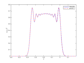
(a) Position Density

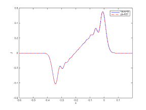
(b) Current Density

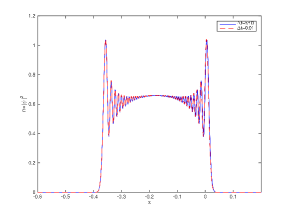
(c) Position Density

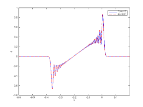
(d) Current Density

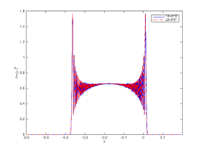
(e) Position Density

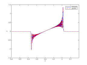
(f) Current Density

Figure 1: Numerical solutions at $T=0.5$ in Example 6.1 computed by the time-splitting method using different meshing strategies. First row: $h=\frac{1}{256}$; Second row: $h=\frac{1}{1024}$; Third row: $h=\frac{1}{4096}$.

4.6in

In addition, we compare the numerical values of $\mu$ computed by $\Delta t=0.01$ and $\Delta t=\frac{h}{10}$ (denoted as $\mu_{1}$ and $\mu_{2}$, respectively). As shown in Table 1, the error is insensitive in $h$, showing a uniform in $h$ convergence in $\Delta t$.

4.6in

$h$	$1/256$	$1/1024$	$1/4096$
$\frac{\left\|\mu_{1}-\mu_{2}\right\|_{\ell^{2}}}{\left\|\mu_{2}\right\|_{\ell^{2}}}$	1.65e-03	1.69e-03	1.70e-03

Table 1: The relative $\ell^{2}-$difference (defined as $\frac{\left\|\mu_{1}-\mu_{2}\right\|_{\ell^{2}}}{\left\|\mu_{2}\right\|_{\ell^{2}}}$) for various $h$.

Example 6.2 (Numerical error as $h$ decreases).

In this example, we choose the same initial data for $\mu_{\rm in}$ as before and

$$\psi_{\rm in}\left(x\right)=\exp\left({-5\left(x+0.1\right)^{2}}\right)\exp\left({\frac{i\sin x}{h}}\right).$$

Now, we fix $\Delta t=$ $0.01$, a stopping time $T=0.4$, and $\Delta y=\Delta\eta=\frac{4\pi}{128}$. We choose $\Delta x=\frac{2\pi h}{16}$, for $h=\frac{1}{64},\frac{1}{128},\frac{1}{256},\frac{1}{512},\frac{1}{1024},\frac{1}{2048}$, respectively. The reference solution is computed with $\Delta t=\frac{h}{10}$. From the $\ell^{2}$-error plotted in Figure 2, one can see that although the error in the wave function increases as $h$ decreases, the error for the position density $|\psi^{h}|^{2}$ as well as for the macroscopic quantity $\mu$ does not change noticeably. This shows that $h-$independent time steps can be taken to accurately obtain physical observables, but not the wave function $\psi^{h}$ itself.

4.6in

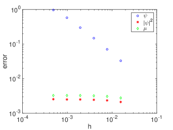
Figure 2: Example 6.2: $\ell^{2}-$errors of the wave function $\psi^{h}$, position density $|\psi^{h}|^{2}$ and $\mu$ for various $h$. Fix $\Delta t=$ $0.01$. For $h=\frac{1}{64},\frac{1}{128},\frac{1}{256},\frac{1}{512},\frac{1}{1024},\frac{1}{2048}$, choose $\Delta x=\frac{2\pi h}{16}$ respectively. The reference solution is computed with $\Delta t=\frac{h}{10}$.

Example 6.3 (Convergence in time).

Finally, to examine the convergence in time of our scheme, let the initial data be as in the example before. Fix $h=$ $\frac{1}{8192}$, a stopping time $T=0.4$ and a spatial discretization with $\Delta x=\frac{2\pi h}{16}$, $\Delta y=\Delta\eta=\frac{4\pi}{128}$. Choose $\Delta t=\frac{0.4}{32},\frac{0.4}{64},\frac{0.4}{128},\frac{0.4}{256},\frac{0.4}{512},\frac{0.4}{1024}$. The reference solution is computed with $\Delta t=\frac{0.4}{81920}$. The $\ell^{2}$-error is plotted in Figure 3, which shows first order accuracy in time of our scheme. Again, we see that the wave function exhibits errors several orders of magnitude larger than the physical observable densities.

4.6in

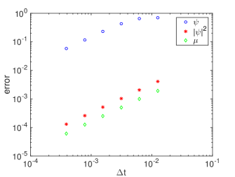
Figure 3: Example 6.3: $\ell^{2}-$errors of the numerical solutions for various $\Delta t$ and fixed $h=\frac{1}{8192}$, $\Delta x=\frac{2\pi h}{16}$, $\Delta y=\Delta\eta=\frac{4\pi}{128}$. It shows first order convergence of the scheme in time. The reference solution is computed with $\Delta t=\frac{0.4}{81920}$.

References

- [1] W. Bao, S. Jin, and P. A. Markowich. On Time-Splitting Spectral Approximations for the Schrödinger Equation in the Semiclassical Regime. J. Comput. Phys., 175(2):487–524, 2002.
- [2] W. Bao, S. Jin, and P. A. Markowich. Numerical study of time-splitting spectral discretizations of nonlinear Schrödinger equations in the semiclassical regimes. SIAM J. Sci. Comput., 25(1):27–64, 2003.
- [3] C. Bayer, H. Hoel, A. Kadir, P. Plecháč, M. Sandberg, and A. Szepessy. Computational error estimates for Born–Oppenheimer molecular dynamics with nearly crossing potential surfaces. Appl. Math. Res. Express, 2015(2):329–417, 2015.
- [4] G. D. Billing. The Quantum Classical Theory. Oxford University Press, 2003.
- [5] R. H. Bisseling, R. Kosloff, R. B. Gerber, M. A. Ratner, L. Gibson, and C. Cerjan. Exact time-dependent quantum mechanical dissociation dynamics of I2He: Comparison of exact time-dependent quantum calculation with the quantum time-dependent self-consistent field (TDSCF) approximation. J. Chem. Phys., 87(5):2760–2765, 1987.
- [6] F. A. Bornemann, P. Nettesheim, and C. Schütte. Quantum-classical molecular dynamics as an approximation to full quantum dynamics. J. Chem. Phys., 105(3):1074–1083, 1996.
- [7] R. Carles. On Fourier time-splitting methods for nonlinear Schrödinger equations in the semiclassical limit. SIAM J. Numerical Anal., 51(6):3232–3258, 2013.
- [8] R. Carles and C. Gallo. On Fourier time-splitting methods for nonlinear Schrödinger equations in the semi-classical limit ii. Analytic regularity. Numer. Math., 136(1):315–342, 2017.
- [9] K. Drukker. Basics of surface hopping in mixed quantum/classical simulations. J. Comput. Phys., 153(2):225–272, 1999.
- [10] P. Ehrenfest. Bemerkung über die angenäherte Gültigkeit der klassischen Mechanik innerhalb der Quantenmechanik. Z. Phys. A, Hadrons Nucl., 45(7):455–457, 1927.
- [11] P. Gerard, P. A. Markowich, N. J. Mauser, and F. Poupaud. Homogenization limits and Wigner transforms. Comm. Pure Appl. Math., 50(4):323–379, 1997.
- [12] S. Jin. Efficient asymptotic-preserving (AP) schemes for some multiscale kinetic equations. SIAM J. Sci. Comput., 21(2):441–454 (electronic), 1999.
- [13] S. Jin. Asymptotic preserving (AP) schemes for multiscale kinetic and hyperbolic equations: a review. Riv. Math. Univ. Parma (N.S.), 3(2):177–216, 2012.
- [14] S. Jin, P. Markowich, and C. Sparber. Mathematical and computational methods for semiclassical Schrödinger equations. Acta Numer., 20:121–209, 2011.
- [15] S. Jin, C. Sparber, and Z. Zhou. On the classical limit of a time-dependent self-consistent field system: Analysis and computation. Kinet. Relat. Models, 10(1):263–298, Mar. 2017.
- [16] Z. Kotler, E. Neria, and A. Nitzan. Multiconfiguration time-dependent self-consistent field approximations in the numerical solution of quantum dynamical problems. Comput.Phys. Comm., 63(1):243–258, 1991.
- [17] Z. Kotler, A. Nitzan, and R. Kosloff. Multiconfiguration time-dependent self-consistent field approximation for curve crossing in presence of a bath. A fast Fourier transform study. Chem. Phys. Lett., 153(6):483–489, 1988.
- [18] R. J. LeVeque. Numerical Methods for Conservation Laws. Birkhäuser Basel, 1992.
- [19] P.-L. Lions and T. Paul. Sur les mesures de Wigner. Rev. Mat. Iberoamericana, 9(3):553–618, 1993.
- [20] N. Makri and W. H. Miller. Time-dependent self-consistent field (TDSCF) approximation for a reaction coordinate coupled to a harmonic bath: Single and multiple configuration treatments. J. Chem. Phys., 87(10):5781–5787, 1987.
- [21] P. A. Markowich and N. J. Mauser. The classical limit of a self-consistent quantum-Vlasov equation in 3d. Math. Models Methods Appl. Sci., 3(01):109–124, 1993.
- [22] D. Marx and J. Hutter. Ab Initio molecular dynamics: Theory and implementation. Modern Meth. Algorithm. Quant. Chem., 1(141):301–449, 2000.
- [23] D. Marx and J. Hutter. Ab Initio Molecular Dynamics: Basic Theory and Advanced Methods. Cambridge University Press, 2009.
- [24] C. Schütte and F. A. Bornemann. On the singular limit of the quantum-classical molecular dynamics model. SIAM J. Appl. Math., 59(4):1208–1224, 1999.
- [25] C. Sparber, P. Markowich, and N. Mauser. Wigner functions versus WKB methods in multivalued geometrical optics. Asymptot. Anal., 33(2):152–187, 2003.
- [26] A. Szepessy. Langevin molecular dynamics derived from Ehrenfest dynamics. Math. Models Methods Appl. Sci., 21(5):2289–2334, 2011.
- [27] M. E. Taylor. Partial Differential Equations: Basic Theory. Applied mathematical sciences. Springer, 1996.
- [28] J. C. Tully. Mixed quantum–classical dynamics. Faraday Discussions, 110:407–419, 1998.
- [29] E. Wigner. On the quantum correction for thermodynamic equilibrium. Phys. Rev., 40(5):749, 1932.