APCTP Pre2017-001

Correlated primordial spectra
in effective theory of inflation

Jinn-Ouk Gong^(a,b) and Masahide Yamaguchi^(c)

^a Asia Pacific Center for Theoretical Physics, Pohang 37673, Korea
^b Department of Physics, POSTECH, Pohang 37673, Korea
^c Department of Physics, Tokyo Institute of Technology, Tokyo 152-8551, Japan

We derive a direct correlation between the power spectrum and bispectrum of the primordial curvature perturbation in terms of the Goldstone mode based on the effective field theory approach to inflation. We show examples of correlated bispectra for the parametrized feature models presented by the Planck collaboration. We also discuss the consistency relation and the validity of our explicit correlation between the power spectrum and bispectrum.

1 Introduction

The high energy scale during inflation, presumably well beyond the reach of the current and future particle accelerator experiments, calls for an effective theory description of inflation [1, 2]. This is because by construction the effective field theory approach is systematic through which we can account for our ignorance. A key observation in writing the effective field theory of single-field inflation is to note that in the time-dependent background the time translational symmetry is broken, while spatial diffeomorphism is preserved [1]. The couplings that determine the expansion of the effective theory of the Goldstone mode $\pi$, which realizes the time diffeomorphism, are represented by a set of mass scales $M_{n}^{4}$. In the so-called decoupling regime the Goldstone $\pi$ could decouple from the metric fluctuations and the effective action of $\pi$ is dramatically simplified. Especially, the first expansion parameter $M_{2}^{4}$ is manifest in both quadratic and cubic order of $\pi$: see (5).

The observation that the coefficient $M_{2}^{4}$ is common to the quadratic and cubic action of $\pi$ indicates that, to leading order in the decoupling limit, the corresponding correlation functions – the power spectrum and bispectrum – are explicitly correlated. It means that ideally, given an explicit analytic form of the power spectrum theoretically, we can find unambiguously the corresponding bispectrum. Or, at the very least observationally, it remains tantalizing because of the existence of outliers in the power spectrum of the temperature fluctuations of the cosmic microwave background [4]. The explicit correlation would make possible joint analysis using the two- and three-point correlation functions [5], which can place much stronger constraints on cosmological parameters. It can also open a compelling way of searching for new physics beyond the paradigm of standard slow-roll inflation, since any deviations would strongly signal the typical mass scale associated with new physics [6].

In this article, we derive a direct and explicit relation between the power spectrum and bispectrum of the primordial curvature perturbation using the Goldstone mode $\pi$. Such a correlation was first explicitly studied in the top-down approach [7] and expanded into more general context in [8], in which heavy degrees of freedom are integrated out to lead to an effective single field description of inflation [9] (see also [10]). To leading order of the heavy mass scale, the speed of sound $c_{s}$ uniquely characterizes the effects of the heavy degrees of freedom [9], i.e. the coefficients of the effective theory. Our approach here is conversely bottom-up, complementary to the previous studies as we will see in the main text.

The article is organized as follows. In the next section, after briefly reviewing the effective field theory of inflation, we derive the simple expression of the correction to the power spectrum. By inverting it we can write the unknown, model-dependent effective theory parameter in terms of the power spectrum which can be constrained observationally. In Section 3, we derive a direct and explicit relation between the corrections of the power spectrum and bispectrum. In Section 4 we discuss the consistency relation of the squeezed bispectrum [11] and the validity of the correlation we derive. The final section is devoted to summary and conclusions.

2 Effective theory and correction to power spectrum

In this section, after briefly reviewing the effective field theory of inflation, we give the formula of the correction to the power spectrum due to the deviation from usual slow-roll phase parametrized by the expansion coefficient of the effective theory.

2.1 Brief review of effective field theory of inflation

We begin with a brief review of the effective field theory of inflation [1]. In unitary gauge, the information on the primordial curvature perturbation is encoded in geometrical quantities respecting the time-dependent spatial diffeomorphism symmetry. Then, the action for the primordial curvature perturbation is written in general as

$$S=\int d^{4}x\sqrt{-g}F(g^{\mu\nu},g_{\mu\nu},K_{\mu\nu},R_{\mu\nu\rho\sigma},\nabla_{\mu},t)\,,$$ (1)

where $K_{\mu\nu}$ is the extrinsic curvature with respect to $t=$ constant hypersurface. Since the zeroth and first order terms are determined by the background quantities, the action can be expanded as

$$S=\int d^{4}x\sqrt{-g} \left\{\frac{1}{2}m_{\rm Pl}^{2}R+m_{\rm Pl}^{2}\dot{H}(t)g^{00}-m_{\rm Pl}^{2}\left[3H^{2}(t)+\dot{H}(t)\right]\right.$$

$$+F\left(\delta g^{00},\delta K_{\mu\nu},\delta R_{\mu\nu\rho\sigma};g_{\mu\nu},g^{\mu\nu},\nabla_{\mu},t\right)\bigg{\}}\,,$$ (2)

where $F$ represents second and higher order perturbation terms and is given by

$$F =\frac{1}{2}M_{2}^{4}(t)\left(\delta g^{00}\right)^{2}+\frac{1}{3!}M_{3}^{4}(t)\left(\delta g^{00}\right)^{3}+\cdots$$

$$\quad-\frac{1}{2}\bar{M}_{1}^{3}(t)\delta g^{00}\delta K-\frac{1}{2}\bar{M}_{2}^{3}(t)K\delta K-\frac{1}{2}\bar{M}_{3}^{3}(t)K^{\mu}{}_{\nu}\delta K^{\nu}{}_{\mu}-\cdots\,,$$ (3)

with $K\equiv K^{\mu}{}_{\mu}$. It is noticed that time diffeomorphism invariance is broken in this action. But, it can be recovered by the introduction of the Stückelberg field $\pi(x)$, which corresponds to the Nambu-Goldstone boson and transforms under the coordinate transformations $t\rightarrow\widetilde{t}=t+\xi^{0}(x)$ and $\textbf{\em x}\rightarrow\widetilde{\textbf{\em x}}$ as

$$\pi(x)\longrightarrow\widetilde{\pi}(\widetilde{x}(x))=\pi(x)-\xi^{0}(x)\,.$$ (4)

In the decoupling regime $H\gtrsim M_{2}^{2}/m_{\rm Pl}$, the action reduces to

$$S_{\pi}=\int d^{4}x\sqrt{-g}\left\{\frac{m_{\rm Pl}^{2}}{2}R-m_{\rm Pl}^{2}\dot{H}\left[\dot{\pi}^{2}-\frac{(\nabla\pi)^{2}}{a^{2}}\right]+2M_{2}^{4}\left[\dot{\pi}^{2}+\dot{\pi}^{3}-\dot{\pi}\frac{(\nabla\pi)^{2}}{a^{2}}\right]-\frac{4}{3}M_{3}^{4}\dot{\pi}^{3}+\cdots\right\}\,,$$ (5)

where the dots represent the higher derivative terms. The sound velocity $c_{s}$ is related to $M_{2}$ as

$$c_{s}^{-2}=1-\frac{2M_{2}^{4}}{m_{\rm Pl}^{2}\dot{H}}\,.$$ (6)

In this article, we further set $M_{3}(t)=0$ because $M_{3}^{4}\sim(1-c_{s}^{-2})M_{2}^{4}$ on general arguments [12]. $\pi$ and ${\cal R}$ are related to linear order by $\pi=-{\cal R}/H$, so in the regime (5) is valid we can to first approximation consider $\dot{\pi}\approx-\dot{\cal R}/H$.

2.2 Corrections to the power spectrum

We first concentrate on the quadratic part and evaluate the correction to power spectrum originating from the term with $M_{2}^{4}$. Since the standard slow-roll terms multiplied by $\dot{H}$ in (5) are dominant as various observations indicate, we treat the quadratic contribution of $M_{2}^{4}$ as perturbation. In terms of the speed of sound (6), we assume that for a limited duration $c_{s}$ deviates from unity, with the deviation being not too far away from unity. Neglecting the metric perturbation as we consider the decoupling regime so that $\sqrt{-g}=a^{3}$ simply, from (5) the quadratic part other than the usual slow-roll, which we may call second order interaction, is

$$S_{\text{2,int}}=\int d^{4}xa^{3}2M_{2}^{4}(t)\dot{\pi}^{2}\,.$$ (7)

The interaction Hamiltonian is then

$$H_{\text{int}}=\int d^{3}xa^{3}(-2)c_{s}^{2}M_{2}^{4}(t)\dot{\pi}^{2}\approx\int d^{3}xa^{3}(-2)M_{2}^{4}(t)\dot{\pi}^{2}\,,$$ (8)

where we have used the assumption that $c_{s}$ is not too far away from unity. This interaction Hamiltonian can be expressed in terms of the Fourier mode as

$$H_{\text{int}}=-2aM_{2}^{4}\int\frac{d^{3}q_{1}d^{3}q_{2}}{(2\pi)^{3}}\delta^{(3)}(-\textbf{\em q}_{12})\pi_{\textbf{\em q}_{1}}^{\prime}\pi_{\textbf{\em q}_{2}}^{\prime}\,,$$ (9)

where $\textbf{\em q}_{12\cdots n}\equiv\textbf{\em q}_{1}+\textbf{\em q}_{2}+\cdots+\textbf{\em q}_{n}$, a prime represents a derivative with respect to the conformal time $d\tau=dt/a$, and

$$\pi(\tau,\textbf{\em x})=\int\frac{d^{3}q}{(2\pi)^{3}}e^{i\textbf{\em q}\cdot\textbf{\em x}}\pi_{\textbf{\em q}}(\tau).$$ (10)

Now we can compute the corrections using the standard in-in formalism. We can straightly obtain

$$\Delta\left\langle\pi_{\textbf{\em k}_{1}}\pi_{\textbf{\em k}_{2}}(\tau)\right\rangle \equiv(2\pi)^{3}\delta^{(3)}(\textbf{\em k}_{12})\frac{2\pi^{2}}{k_{1}^{3}}\Delta{\cal P}_{\pi}$$

$$=i\int_{\tau_{0}\to-\infty}^{\tau\to 0}ad\tau^{\prime}\left\langle 0\left|\left[H_{\text{int}}(\tau^{\prime}),\pi_{\textbf{\em k}_{1}}\pi_{\textbf{\em k}_{2}}(\tau)\right]\right|0\right\rangle$$

$$=(2\pi)^{3}\delta^{(3)}(\textbf{\em k}_{12})2\Re\left[2i\widehat{\pi}_{{k}_{1}}^{*}\widehat{\pi}_{{k}_{2}}^{*}(0)\int_{-\infty}^{0}d\tau\left(-2a^{2}M_{2}^{4}\right)\widehat{\pi}_{{k}_{1}}^{\prime}\widehat{\pi}_{{k}_{2}}^{\prime}(\tau)\right]\,,$$ (11)

where we have expanded the free field $\pi_{\textbf{\em k}}$ using the creation and annihilation operators as

$$\pi_{\textbf{\em k}}=a_{\textbf{\em k}}\widehat{\pi}_{k}+a_{-\textbf{\em k}}^{\dagger}\widehat{\pi}_{k}^{*}\quad\text{with}\quad\left[a_{\textbf{\em k}},a_{\textbf{\em q}}^{\dagger}\right]=(2\pi)^{3}\delta^{(3)}(\textbf{\em k}-\textbf{\em q})\,,$$ (12)

and $\widehat{\pi}_{k}(\tau)$ is the mode function solution given by

$$\widehat{\pi}_{k}(\tau)=-\frac{\widehat{{\cal R}}_{k}}{H}=\frac{-i}{\sqrt{4\epsilon k^{3}}m_{\rm Pl}}(1+ik\tau)e^{-ik\tau}\,.$$ (13)

Thus, we immediately find the correction to the power spectrum as

$$\frac{\Delta{\cal P}_{\pi}}{{\cal P}_{\pi}}(k)\approx\frac{\Delta{\cal P}_{\cal R}}{{\cal P}_{\cal R}}(k)\approx\frac{k}{m_{\rm Pl}^{2}\epsilon H^{2}}\int_{-\infty}^{0}d\tau\left(-2M_{2}^{4}\right)\sin(2k\tau)\,,$$ (14)

where

$${\cal P}_{\pi}=\frac{{\cal P}_{\cal R}}{H^{2}}=\frac{1}{8\pi^{2}m_{\rm Pl}^{2}\epsilon}$$ (15)

is the featureless flat spectrum.

2.3 Inverting the power spectrum

For future convenience, let us return to (2.2) and write it in an alternative form. The real part is obtained by adding the complex conjugate:

$$\frac{2\pi^{2}}{k_{1}^{3}}\Delta{\cal P}_{\pi} =2\Re\left[2i\widehat{\pi}_{{k}_{1}}^{*}\widehat{\pi}_{{k}_{2}}^{*}(0)\int_{-\infty}^{0}d\tau\left(-2a^{2}M_{2}^{4}\right)\widehat{\pi}_{{k}_{1}}^{\prime}\widehat{\pi}_{{k}_{2}}^{\prime}(\tau)\right]$$

$$=2i\widehat{\pi}_{{k}_{1}}^{*}\widehat{\pi}_{{k}_{2}}^{*}(0)\int_{-\infty}^{0}d\tau\left(-2a^{2}M_{2}^{4}\right)\widehat{\pi}_{{k}_{1}}^{\prime}\widehat{\pi}_{{k}_{2}}^{\prime}(\tau)+c.c.\,.$$ (16)

By noting from (13) that $\widehat{\pi}_{k}(-\tau)=-\widehat{\pi}_{k}^{*}(\tau)$ and $\widehat{\pi}_{k}^{\prime}(-\tau)={\widehat{\pi}_{k}}^{*}(\tau)$, and by oddly extending $M_{2}^{4}$ to define $\widetilde{M}_{2}^{4}$ as

$$\widetilde{M}_{2}^{4}(\tau)\equiv\left\{\begin{array}[]{ll}M_{2}^{4}(\tau)&\text{ if }\tau<0\\ -M_{2}^{4}(-\tau)&\text{ if }\tau>0\end{array}\right.\,,$$ (17)

(2.3) can be written as

$$\frac{2\pi^{2}}{k_{1}^{3}}\Delta{\cal P}_{\pi} =2i\widehat{\pi}_{{k}_{1}}^{*}\widehat{\pi}_{{k}_{2}}^{*}(0)\int_{-\infty}^{\infty}d\tau\left(-2a^{2}\widetilde{M}_{2}^{4}\right)\widehat{\pi}_{{k}_{1}}^{\prime}\widehat{\pi}_{{k}_{2}}^{\prime}(\tau)$$

$$=2\pi^{2}{\cal P}_{\pi}\frac{1}{k_{1}k_{2}}\frac{1}{2}\int_{-\infty}^{\infty}d\tau\frac{-2\widetilde{M}_{2}^{4}}{\epsilon m_{\rm Pl}^{2}H^{2}}ie^{-ik_{12}\tau}\,.$$ (18)

Since we have defined $\widetilde{M}_{2}^{4}$ oddly, only the odd part of $e^{-ik_{12}\tau}$ survives and finally we have, setting $k_{1}=k_{2}=k$,

$$\frac{\Delta{\cal P}_{\pi}}{{\cal P}_{\pi}}=\frac{k}{2}\int_{-\infty}^{\infty}d\tau\frac{-2\widetilde{M}_{2}^{4}}{\epsilon m_{\rm Pl}^{2}H^{2}}\sin(2k\tau)\,.$$ (19)

From (19) we can write the coefficient $\widetilde{M}_{2}^{4}$, which is essentially $M_{2}^{4}$ in the effective action (5), in terms of $\Delta{\cal P}_{\pi}/{\cal P}_{\pi}$ as follows. From $\sin(2k\tau)=\left(e^{2ik\tau}-e^{-2ik\tau}\right)/(2i)$, we can multiply $e^{2ik\tau^{\prime}}$ to both sides of (19) and integrate over $k$ to obtain

$$\int_{-\infty}^{\infty}dke^{2ik\tau^{\prime}}\frac{2i}{k}\epsilon m_{\rm Pl}^{2}H^{2}\frac{\Delta{\cal P}_{\cal R}}{{\cal P}_{\cal R}}(k)=\frac{1}{2}\int_{-\infty}^{\infty}d\tau\left(-2\widetilde{M}_{2}^{4}\right)\int_{-\infty}^{\infty}dk\left[e^{2ik(\tau+\tau^{\prime})}-e^{-2ik(\tau-\tau^{\prime})}\right]=2\pi\widetilde{M}_{2}^{4}(\tau^{\prime})\,.$$ (20)

Thus,

$$2\widetilde{M}_{2}^{4}(\tau)=i\frac{2\epsilon m_{\rm Pl}^{2}H^{2}}{\pi}\int_{-\infty}^{\infty}\frac{dk}{k}\frac{\Delta{\cal P}_{\cal R}}{{\cal P}_{\cal R}}(k)e^{2ik\tau}\,.$$ (21)

This is the inverse formula, in which $M_{2}^{4}$ can be expressed in terms of the correction to power spectrum.

3 Correlation between power spectrum and bispectrum

In this section, we first give the formula of bispectrum coming from the cubic action (5), and then derive the explicit relation between the correction to the power spectrum and the bispectrum.

3.1 Bispectrum

As advertised before, we only consider the cubic order action with the coefficient $M_{2}^{4}$:

$$S_{3}=\int d^{4}x\sqrt{-g}2M_{2}^{4}\left[\dot{\pi}^{3}-\dot{\pi}\frac{(\nabla\pi)^{2}}{a^{2}}\right]\,.$$ (22)

We can follow the same steps as before: the interaction Hamiltonian is

$$H_{\text{int}} =-\int d^{3}xa^{3}\cdot 2M_{2}^{4}\left[\dot{\pi}^{3}-\dot{\pi}\frac{(\nabla\pi)^{2}}{a^{2}}\right]$$

$$=-2a^{3}M_{2}^{4}\int\frac{d^{3}q_{1}d^{3}q_{2}d^{3}q_{3}}{(2\pi)^{3\cdot 2}}\delta^{(3)}(-\textbf{\em q}_{123})\left[\dot{\pi}_{\textbf{\em q}_{1}}\dot{\pi}_{\textbf{\em q}_{2}}\dot{\pi}_{\textbf{\em q}_{3}}+\frac{\textbf{\em q}_{1}\cdot\textbf{\em q}_{2}}{3a^{2}}\pi_{\textbf{\em q}_{1}}\pi_{\textbf{\em q}_{2}}\dot{\pi}_{\textbf{\em q}_{3}}+\text{2 perm}\right]\,.$$ (23)

Then, the bispectrum of $\pi$ becomes

$$\left\langle\pi_{\textbf{\em k}_{1}}\pi_{\textbf{\em k}_{2}}\pi_{\textbf{\em k}_{3}}(\tau)\right\rangle \equiv(2\pi)^{3}\delta^{(3)}(\textbf{\em k}_{123})B_{\pi}(\textbf{\em k}_{1},\textbf{\em k}_{2},\textbf{\em k}_{3})$$

$$=(2\pi)^{3}\delta^{(3)}(\textbf{\em k}_{123})\left\{i\widehat{\pi}_{k_{1}}^{*}\widehat{\pi}_{k_{2}}^{*}\widehat{\pi}_{k_{3}}^{*}(0)\int_{-\infty}^{0}d\tau\left(-2aM_{2}^{4}\right)\right.$$

$$\qquad\qquad\qquad\qquad\times\Bigl{[}6\widehat{\pi}_{q_{1}}^{\prime}\widehat{\pi}_{q_{2}}^{\prime}\widehat{\pi}_{q_{3}}^{\prime}(\tau)+2(\textbf{\em k}_{1}\cdot\textbf{\em k}_{2})\widehat{\pi}_{q_{1}}\widehat{\pi}_{q_{2}}\widehat{\pi}_{q_{3}}^{\prime}(\tau)+\text{2 perm}\Bigr{]}+c.c.\biggr{\}}\,.$$ (24)

Again, we can find that by extending $M_{2}^{4}$ oddly the complex conjugate includes the integral from 0 to $\infty$, so

$$B_{\pi}(\textbf{\em k}_{1},\textbf{\em k}_{2},\textbf{\em k}_{3})=i\widehat{\pi}_{k_{1}}^{*}\widehat{\pi}_{k_{2}}^{*}\widehat{\pi}_{k_{3}}^{*}(0)\int_{-\infty}^{\infty}d\tau\left(-2a\widetilde{M}_{2}^{4}\right)\left[6\widehat{\pi}_{q_{1}}^{\prime}\widehat{\pi}_{q_{2}}^{\prime}\widehat{\pi}_{q_{3}}^{\prime}(\tau)+2(\textbf{\em k}_{1}\cdot\textbf{\em k}_{2})\widehat{\pi}_{q_{1}}\widehat{\pi}_{q_{2}}\widehat{\pi}_{q_{3}}^{\prime}(\tau)+\text{2 perm}\right]\,.$$ (25)

3.2 Bispectrum in terms of the power spectrum

In this subsection, we can use (21) and write the bispectrum (25) purely in terms of the power spectrum and its derivatives. Let us first consider the first term of (25). We can straightforwardly write, with $K\equiv k_{123}$,

$$i\widehat{\pi}_{k_{1}}^{*}\widehat{\pi}_{k_{2}}^{*}\widehat{\pi}_{k_{3}}^{*}(0) \int_{-\infty}^{\infty}d\tau\left(-2a\widetilde{M}_{2}^{4}\right)6\widehat{\pi}_{q_{1}}^{\prime}\widehat{\pi}_{q_{2}}^{\prime}\widehat{\pi}_{q_{3}}^{\prime}(\tau)=(2\pi^{2}{\cal P}_{\pi})^{2}\frac{H}{\pi}\frac{3H}{k_{1}k_{2}k_{3}}\int_{-\infty}^{\infty}\frac{dk}{k}\frac{\Delta{\cal P}_{\cal R}}{{\cal P}_{\cal R}}(k)\int_{-\infty}^{\infty}d\tau\tau^{2}e^{i(2k-K)\tau}$$

$$=(2\pi^{2}{\cal P}_{\pi})^{2}\frac{3}{4}H\frac{1}{k_{1}k_{2}k_{3}}\int_{-\infty}^{\infty}\frac{dk}{k}\frac{\Delta{\cal P}_{\cal R}}{{\cal P}_{\cal R}}(k)\frac{d^{2}}{dk^{2}}\delta\left(k-\frac{K}{2}\right)$$

$$=(2\pi^{2}{\cal P}_{\pi})^{2}\frac{3}{4}H\frac{1}{k_{1}k_{2}k_{3}}\frac{d^{2}}{dk^{2}}\left.\left[\frac{1}{k}\frac{\Delta{\cal P}_{\cal R}}{{\cal P}_{\cal R}}(k)\right]\right|_{k=K/2}\,,$$ (26)

where for the second equality we have replaced $\tau^{2}$ in the time integral with two derivatives with respect to $k$, and for the last equality we have iteratively integrated by parts.

To proceed further, with ${\cal P}_{\cal R}^{\text{(total)}}={\cal P}_{\cal R}+\Delta{\cal P}_{\cal R}$, from

$$\log{\cal P}_{\cal R}^{\text{(total)}}\approx\log{\cal P}_{\cal R}+\frac{\Delta{\cal P}_{\cal R}}{{\cal P}_{\cal R}}\,,$$ (27)

with ${\cal P}_{\cal R}$ being flat, we can find the spectral index and the running respectively as

$$n_{\cal R}-1 \equiv\frac{d\log{\cal P}_{\cal R}^{\text{(total)}}}{d\log{k}}=k\frac{d}{dk}\left(\frac{\Delta{\cal P}_{\cal R}}{{\cal P}_{\cal R}}\right)\,,$$ (28)

$$\alpha_{\cal R} \equiv\frac{dn_{\cal R}}{d\log{k}}=k^{2}\frac{d^{2}}{dk^{2}}\left(\frac{\Delta{\cal P}_{\cal R}}{{\cal P}_{\cal R}}\right)+k\frac{d}{dk}\left(\frac{\Delta{\cal P}_{\cal R}}{{\cal P}_{\cal R}}\right)\,.$$ (29)

Thus (3.2) can be now written as

$$i\widehat{\pi}_{k_{1}}^{*}\widehat{\pi}_{k_{2}}^{*}\widehat{\pi}_{k_{3}}^{*}(0)\int_{-\infty}^{\infty}d\tau\left(-2a\widetilde{M}_{2}^{4}\right)6\widehat{\pi}_{q_{1}}^{\prime}\widehat{\pi}_{q_{2}}^{\prime}\widehat{\pi}_{q_{3}}^{\prime}(\tau)$$

$$\qquad\qquad=(2\pi)^{4}{\cal P}_{\pi}^{2}\frac{3}{2}H\frac{1}{k_{1}k_{2}k_{3}}\frac{1}{K^{3}}\left[\alpha_{\cal R}-3(n_{\cal R}-1)+2\frac{\Delta{\cal P}_{\cal R}}{{\cal P}_{\cal R}}\right]\bigg{|}_{k=K/2}\,.$$ (30)

We can proceed in a similar manner for the second term of (25) and find

$$i\widehat{\pi}_{k_{1}}^{*}\widehat{\pi}_{k_{2}}^{*}\widehat{\pi}_{k_{3}}^{*}(0)\int_{-\infty}^{\infty}d\tau\left(-2a\widetilde{M}_{2}^{4}\right)2(\textbf{\em k}_{1}\cdot\textbf{\em k}_{2})\widehat{\pi}_{q_{1}}\widehat{\pi}_{q_{2}}\widehat{\pi}_{q_{3}}^{\prime}(\tau)$$

$$=(2\pi)^{4}{\cal P}_{\pi}^{2}\frac{1}{H}\frac{-\textbf{\em k}_{1}\cdot\textbf{\em k}_{2}}{(k_{1}k_{2})^{3}k_{3}}\left[\left(1+\frac{k_{12}}{K}+\frac{2k_{1}k_{2}}{K^{2}}\right)\frac{\Delta{\cal P}_{\cal R}}{{\cal P}_{\cal R}}+\left(-\frac{k_{12}}{K}-\frac{3k_{1}k_{2}}{K^{2}}\right)(n_{\cal R}-1)+\frac{k_{1}k_{2}}{K^{2}}\alpha_{\cal R}\right]\bigg{|}_{k=K/2}\,.$$ (31)

Thus, the bispectrum can be expressed in terms of the correction to power spectrum, its first and second derivatives as

$$B_{\pi}(\textbf{\em k}_{1},\textbf{\em k}_{2},\textbf{\em k}_{3})$$

$$=(2\pi)^{4}{\cal P}_{\pi}^{2}\frac{H}{(k_{1}k_{2}k_{3})^{3}}\left[{A}(k_{1},k_{2},k_{3})\frac{\Delta{\cal P}_{\cal R}}{{\cal P}_{\cal R}}+{B}(k_{1},k_{2},k_{3})(n_{\cal R}-1)+{C}(k_{1},k_{2},k_{3})\alpha_{\cal R}\right]\bigg{|}_{k=K/2}\,,$$ (32)

where the functions of momenta ${A}$, ${B}$ and ${C}$ are given by, respectively,

$${A}(k_{1},k_{2},k_{3}) =-\frac{1}{K^{2}}\sum_{i\neq j}k_{i}^{2}k_{j}^{3}+2\frac{1}{K}\sum_{i>j}k_{i}^{2}k_{j}^{2}-\frac{1}{4}\sum_{i}k_{i}^{3}\,,$$ (33)

$${B}(k_{1},k_{2},k_{3}) =2\frac{1}{K^{2}}\sum_{i\neq j}k_{i}^{2}k_{j}^{3}-3\frac{1}{K}\sum_{i>j}k_{i}^{2}k_{j}^{2}+\frac{1}{4}\sum_{i\neq j}k_{i}k_{j}^{2}-\frac{1}{4}k_{1}k_{2}k_{3}\,,$$ (34)

$${C}(k_{1},k_{2},k_{3}) =-\frac{1}{K^{2}}\sum_{i\neq j}k_{i}^{2}k_{j}^{3}+\frac{1}{K}\sum_{i>j}k_{i}^{2}k_{j}^{2}-\frac{1}{4}k_{1}k_{2}k_{3}\,.$$ (35)

This expression is one of the main results in this article.

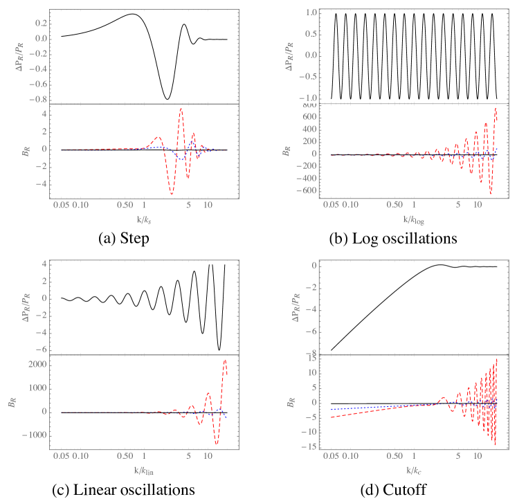
Figure 1: (Upper panels) power spectrum and (lower panels) the corresponding bispectrum for various feature models (36) discussed in [13]. For simplicity, we have set the amplitudes of the features as $A_{s}=A_{\text{log}}=A_{\text{lin}}=1$ and phases as $\varphi_{\text{log}}=\varphi_{\text{in}}=0$. For the step model, we have also set the damping scale $x_{d}=1$. Meanwhile, following [13] we have set $\log_{10}\omega_{\text{log}}=1.25$, $\log_{10}\omega_{\text{lin}}=1.02$ and $n_{\text{lin}}=0.66$. We show the bispectrum projected onto the equilateral (red dashed), folded (blue dotted) and squeezed (black solid) configurations.

In Figure 1, we show a few examples using the following parametrized feature models [13]: a localized oscillatory burst due to e.g. step in the inflaton potential, logarithmic and linear oscillations and cutoff models given by

$$\frac{\Delta{\cal P}_{\cal R}}{{\cal P}_{\cal R}}=\left\{\begin{array}[]{ll}A_{s}W_{0}\left(\dfrac{k}{k_{s}}\right)D\left(\dfrac{k/k_{s}}{x_{d}}\right)&\text{(step)}\\ A_{\text{log}}\cos\left[\omega_{\text{log}}\log\left(\dfrac{k}{k_{\text{log}}}\right)+\varphi_{\text{log}}\right]&\text{(logarithmic oscillations)}\\ A_{\text{lin}}\left(\dfrac{k}{k_{\text{lin}}}\right)^{n_{\text{lin}}}\cos\left(\omega_{\text{lin}}\dfrac{k}{k_{\text{lin}}}+\varphi_{\text{lin}}\right)&\text{(linear oscillations)}\\ \log\left(\dfrac{\pi}{16}\dfrac{k}{k_{c}}|C_{c}-D_{c}|^{2}\right)&\text{(cutoff model)}\end{array}\right.\,,$$ (36)

where the functions that appear in these parametrized feature models are

$$W_{0}(x) =\frac{1}{2x^{4}}\Big{[}\left(18x-6x^{3}\right)\cos(2x)+\left(15x^{2}-9\right)\sin(2x)\Big{]}\,,$$ (37)

$$D(x) =\frac{x}{\sinh{x}}\,,$$ (38)

$$C_{c} =\exp\left(\frac{-ik}{k_{c}}\right)\left[H_{0}^{(2)}\left(\frac{k}{2k_{c}}\right)-\left(\frac{1}{k/k_{c}}+i\right)H_{1}^{(2)}\left(\frac{k}{2k_{c}}\right)\right]\,,$$ (39)

$$D_{c} =\exp\left(\frac{ik}{k_{c}}\right)\left[H_{0}^{(2)}\left(\frac{k}{2k_{c}}\right)-\left(\frac{1}{k/k_{c}}-i\right)H_{1}^{(2)}\left(\frac{k}{2k_{c}}\right)\right]\,,$$ (40)

with $H_{n}^{(2)}$ being the Hankel function of the second kind. As we can see, each power spectrum gives distinctively different patterns of the corresponding bispectrum in various configurations.

4 Squeezed bispectrum and consistency relation

We can note that (3.2) vanishes in the squeezed limit, say, $k_{1}\approx k_{2}$ and $k_{3}\to 0$. This seems to contradict the consistency relation between the power spectrum and the squeezed limit of the bispectrum [11],

$$B_{\cal R}(k_{1},k_{2},k_{3})\underset{k_{3}\to 0}{\longrightarrow}(1-n_{\cal R})P_{\cal R}(k_{1})P_{\cal R}(k_{3})\,,$$ (41)

because as (14) shows the power spectrum is well away from featureless flat one, so the corresponding spectral index is non-trivial. Indeed, in [7], the consistency relation is recovered for features caused by non-trivial speed of sound.

Let us first return to the quadratic action for the curvature perturbation. Including the speed of sound, it is written as

$$S_{2}=\int d^{4}xa^{3}m_{\rm Pl}^{2}\epsilon\left[\frac{\dot{\cal R}^{2}}{c_{s}^{2}}-\frac{(\nabla{\cal R})^{2}}{a^{2}}\right]\,,$$ (42)

so there are two possible sources of departure from the usual canonical slow-roll [15]: $\epsilon$ and $c_{s}$. Let us consider these two cases separately. Our goal here is to see the form of the corrections to the power spectrum for each case. But this seems unclear, since the form of the interaction part of the quadratic action – just $\dot{\cal R}^{2}$ for $c_{s}$, and $\dot{\cal R}^{2}$ and $(\nabla{\cal R})^{2}$ for $\epsilon$ – is different. Thus naively thinking the resulting correction terms would be of different structure. We first assume that $c_{s}$ solely supplies the deviations from the standard slow-roll in such a way that for a limited duration $c_{s}$ deviates from unity, with the deviation being not too far away from unity. We may then write, with the canonical slow-roll part being the leading, free part,

$$S_{2}=\int d^{4}xa^{3}m_{\rm Pl}^{2}\epsilon\left[\dot{\cal R}^{2}-\frac{(\nabla{\cal R})^{2}}{a^{2}}\right]+\underbrace{\int d^{4}xa^{3}m_{\rm Pl}^{2}\epsilon\left(\frac{1}{c_{s}^{2}}-1\right)}_{\equiv S_{\text{2,int}}}\,.$$ (43)

Following the same steps as in Section 2.2, we find

$$\frac{\Delta{\cal P}_{\cal R}}{{\cal P}_{\cal R}}=k\int_{-\infty}^{0}d\tau\left(c_{s}^{2}-1\right)\sin(2k\tau)\,,$$ (44)

which is of the same structure as (14).

For the case in which $\epsilon$ is responsible for the departure from the standard slow-roll, let us split $\epsilon$ into the slowly varying part $\epsilon_{0}$ and the rapidly varying but transient part $\Delta\epsilon$:

$$\epsilon=\epsilon_{0}+\Delta\epsilon\,.$$ (45)

We can rewrite $\Delta\epsilon$ as

$$\Delta\epsilon=\int\dot{\epsilon}dt\approx H\epsilon_{0}\int\eta dt\approx\epsilon_{0}\eta H\Delta t\,,$$ (46)

where $\Delta t={\cal O}(1/H)$ is the duration of departure and we have defined another slow-roll parameter $\eta\equiv\dot{\epsilon}/(H\epsilon)$. Then the quadratic action (42), with $c_{s}=1$ this time, can be written as

$$S_{2}=\int d^{4}xa^{3}m_{\rm Pl}^{2}\epsilon_{0}\left[\dot{\cal R}^{2}-\frac{(\nabla{\cal R})^{2}}{a^{2}}\right]+\underbrace{\int d^{4}xa^{3}m_{\rm Pl}^{2}\Delta\epsilon\left[\dot{\cal R}^{2}-\frac{(\nabla{\cal R})^{2}}{a^{2}}\right]}_{\equiv S_{\text{2,int}}}\,,$$ (47)

and the corresponding correction to the power spectrum is

$$\frac{\Delta{\cal P}_{\cal R}}{{\cal P}_{\cal R}}=k\int_{-\infty}^{0}d\tau\left(-2\frac{\Delta\epsilon}{\epsilon_{0}}\right)\sin(2k\tau)\,.$$ (48)

Comparing this with (44), we see that two sources of the departure from the standard slow-roll leads to the same structure of the correction as (14). This seems to suggest that indeed $M_{2}^{4}$ captures the deviation from usual slow-roll on general ground.

We now return to our starting equation (5) to clarify this inconsistency. A key observation is that unlike ${\cal R}$, which is frozen on super-horizon scales, $\pi$ evolves as

$$\dot{\pi}=-\frac{\dot{\cal R}}{H}-\epsilon{\cal R}+\frac{\dot{\cal R}^{2}}{H^{2}}+3\epsilon\frac{\dot{\cal R}{\cal R}}{H}+\cdots\,,$$ (49)

where the non-linear terms follow from the fact that essentially $\pi$ is the time translation between spatially flat and comoving hypersurfaces [16]. Also we have omitted terms that are further suppressed in slow-roll parameters. Taking into account the sub-leading terms in $\dot{\pi}$, at quadratic order of the curvature perturbation $M_{2}^{4}$ contributes

$$S_{\cal R}\supset\int d^{4}a^{3}\left[\frac{2M_{2}^{4}}{H^{2}}\dot{\cal R}^{2}+2\epsilon\left(-3M_{2}^{4}+\frac{\dot{M}_{2}^{4}}{H}\right){\cal R}^{2}\right]\,.$$ (50)

Thus, the speed of sound of the curvature perturbation is identical to that of $\pi$ given by (6). At the same time there do exist changes in ${\cal R}^{2}$ terms as (47), but they are slow-roll suppressed. Since we have only considered the leading effects that only capture the speed of sound, the bispectrum (3.2) is enhanced in the equilateral configuration while it is not in the squeezed limit. Indeed, by considering the sub-leading terms in (49), we have at cubic order new terms $\dot{\cal R}^{2}{\cal R}$ and ${\cal R}(\nabla{\cal R})^{2}$ that lead to non-vanishing bispectrum in the squeezed limit [17]. More specifically, the new terms $\dot{\cal R}^{2}{\cal R}$ and ${\cal R}(\nabla{\cal R})^{2}$ in the cubic order action give up to numerical coefficient

$$\frac{k_{1}k_{2}k_{3}}{k_{1}^{3}+k_{2}^{3}+k_{3}^{3}}\frac{(k_{1}k_{2}k_{3})^{2}B_{\cal R}(k_{1},k_{2},k_{3})}{(2\pi)^{4}{\cal P}_{\cal R}^{2}}\underset{k_{3}\to 0}{\longrightarrow}\epsilon\frac{\Delta{\cal P}_{\cal R}}{{\cal P}_{\cal R}}\,,$$ (51)

with $k_{1}\approx k_{2}\equiv k$. Still the consistency relation is not recovered, but this is because we are not taking into account all the next-to-leading terms in the decoupling limit, such as the modification of the mode functions: terms of ${\cal O}(1/c_{s}^{2})$ and ${\cal O}(\epsilon/c_{s}^{2})$ do not contribute to the squeezed limit while only terms of ${\cal O}(\epsilon)$ do [18]. Our calculation is done only up to the leading order.

5 Summary

In this article, we have derived the direct relation between the corrections of power spectrum and bispectrum of the primordial curvature perturbation. Our formula is based on the effective field theory approach to inflation, which to first approximation captures the effects of the non-trivial speed of sound. If we would observationally detect the deviation from the standard slow-roll inflation, it is important to check the relation derived here, which could prove/disprove whether such a deviation can be attributed to the variation of sound velocity.

We have also shown that the corrections to the power spectrum from non-trivial features of sound velocity and expansion rate of the universe, which characterize the deviation from the standard slow-roll inflation, have the same form. It is interesting to check whether we can extend this kind of unified treatment to higher order correlation functions. We have also discussed the squeezed limit of the bispectrum and the consistency relation. In the leading order calculations we have adopted in this article, the squeezed limit vanishes. But, if we take into account sub-leading orders adequately, the consistency relation would be recovered.

The next step is to include the sub-leading order effects such as the terms beyond decoupling limit and the $M_{3}$ terms. Then, we will have further (consistency) relation, which is useful to identify new physics causing such a deviation.

Acknowledgments

JG thanks Tokyo Institute of Technology for hospitality during “Workshop on Particle Physics, Cosmology, and Gravitation” where this work was initiated. JG acknowledges the support from the Korea Ministry of Education, Science and Technology, Gyeongsangbuk-Do and Pohang City for Independent Junior Research Groups at the Asia Pacific Center for Theoretical Physics. JG is also supported in part by a TJ Park Science Fellowship of POSCO TJ Park Foundation and the Basic Science Research Program through the National Research Foundation of Korea (NRF) Research Grant NRF-2016R1D1A1B03930408. MY is supported in part by Japan Society for the Promotion of Science (JSPS) Grant-in-Aid for Scientific Research Nos. 25287054 and 26610062, and the Grant-in-Aid for Scientific Research on Innovative Areas “Cosmic Acceleration” No. 15H05888.

References

- [1] C. Cheung, P. Creminelli, A. L. Fitzpatrick, J. Kaplan and L. Senatore, JHEP 0803, 014 (2008) [arXiv:0709.0293 [hep-th]].
- [2] S. Weinberg, Phys. Rev. D 77, 123541 (2008) [arXiv:0804.4291 [hep-th]].
- [3] L. Senatore and M. Zaldarriaga, JHEP 1204, 024 (2012) [arXiv:1009.2093 [hep-th]] ; T. Noumi, M. Yamaguchi and D. Yokoyama, JHEP 1306, 051 (2013) [arXiv:1211.1624 [hep-th]].
- [4] S. L. Bridle, A. M. Lewis, J. Weller and G. Efstathiou, Mon. Not. Roy. Astron. Soc. 342, L72 (2003) [astro-ph/0302306] ; A. Shafieloo, T. Souradeep, P. Manimaran, P. K. Panigrahi and R. Rangarajan, Phys. Rev. D 75, 123502 (2007) [astro-ph/0611352] ; D. K. Hazra, A. Shafieloo and T. Souradeep, JCAP 1411, no. 11, 011 (2014) [arXiv:1406.4827 [astro-ph.CO]] ; P. Hunt and S. Sarkar, JCAP 1512, no. 12, 052 (2015) [arXiv:1510.03338 [astro-ph.CO]].
- [5] A. Achucarro, V. Atal, P. Ortiz and J. Torrado, Phys. Rev. D 89, no. 10, 103006 (2014) [arXiv:1311.2552 [astro-ph.CO]] ; A. Achucarro, V. Atal, B. Hu, P. Ortiz and J. Torrado, Phys. Rev. D 90, no. 2, 023511 (2014) [arXiv:1404.7522 [astro-ph.CO]] ; J. R. Fergusson, H. F. Gruetjen, E. P. S. Shellard and M. Liguori, Phys. Rev. D 91, no. 2, 023502 (2015) [arXiv:1410.5114 [astro-ph.CO]] ; J. R. Fergusson, H. F. Gruetjen, E. P. S. Shellard and B. Wallisch, Phys. Rev. D 91, no. 12, 123506 (2015) [arXiv:1412.6152 [astro-ph.CO]] ; P. D. Meerburg, M. Munchmeyer and B. Wandelt, Phys. Rev. D 93, no. 4, 043536 (2016) [arXiv:1510.01756 [astro-ph.CO]] ; S. Appleby, J. O. Gong, D. K. Hazra, A. Shafieloo and S. Sypsas, Phys. Lett. B 760, 297 (2016) [arXiv:1512.08977 [astro-ph.CO]].
- [6] D. Baumann and D. Green, JCAP 1109, 014 (2011) [arXiv:1102.5343 [hep-th]] ; A. Achucarro, J. O. Gong, S. Hardeman, G. A. Palma and S. P. Patil, JHEP 1205, 066 (2012) [arXiv:1201.6342 [hep-th]].
- [7] A. Achucarro, J. O. Gong, G. A. Palma and S. P. Patil, Phys. Rev. D 87, no. 12, 121301 (2013) [arXiv:1211.5619 [astro-ph.CO]]. See for earlier references e.g. X. Chen, R. Easther and E. A. Lim, JCAP 0706, 023 (2007) [astro-ph/0611645] ; X. Chen, R. Easther and E. A. Lim, JCAP 0804, 010 (2008) [arXiv:0801.3295 [astro-ph]].
- [8] J. O. Gong, K. Schalm and G. Shiu, Phys. Rev. D 89, no. 6, 063540 (2014) [arXiv:1401.4402 [astro-ph.CO]].
- [9] A. J. Tolley and M. Wyman, Phys. Rev. D 81, 043502 (2010) [arXiv:0910.1853 [hep-th]] ; A. Achucarro, J. O. Gong, S. Hardeman, G. A. Palma and S. P. Patil, Phys. Rev. D 84, 043502 (2011) [arXiv:1005.3848 [hep-th]] ; A. Achucarro, J. O. Gong, S. Hardeman, G. A. Palma and S. P. Patil, JCAP 1101, 030 (2011) [arXiv:1010.3693 [hep-ph]] ; A. Achucarro, V. Atal, S. Cespedes, J. O. Gong, G. A. Palma and S. P. Patil, Phys. Rev. D 86, 121301 (2012) [arXiv:1205.0710 [hep-th]].
- [10] G. Shiu and J. Xu, Phys. Rev. D 84, 103509 (2011) [arXiv:1108.0981 [hep-th]] ; X. Gao, D. Langlois and S. Mizuno, JCAP 1210, 040 (2012) [arXiv:1205.5275 [hep-th]] ; R. Saito, M. Nakashima, Y. i. Takamizu and J. Yokoyama, JCAP 1211, 036 (2012) [arXiv:1206.2164 [astro-ph.CO]] ; R. Saito and Y. i. Takamizu, JCAP 1306, 031 (2013) [arXiv:1303.3839, arXiv:1303.3839 [astro-ph.CO]] ; X. Gao, D. Langlois and S. Mizuno, JCAP 1310, 023 (2013) [arXiv:1306.5680 [hep-th]] ; T. Noumi and M. Yamaguchi, JCAP 1312, 038 (2013) [arXiv:1307.7110 [hep-th]] ; M. Konieczka, R. H. Ribeiro and K. Turzynski, JCAP 1407, 030 (2014) [arXiv:1401.6163 [astro-ph.CO]] ; T. Battefeld and R. C. Freitas, JCAP 1409, 029 (2014) [arXiv:1405.7969 [astro-ph.CO]] ; X. Gao and J. O. Gong, JHEP 1508, 115 (2015) [arXiv:1506.08894 [astro-ph.CO]].
- [11] J. M. Maldacena, JHEP 0305, 013 (2003) [astro-ph/0210603] ; P. Creminelli and M. Zaldarriaga, JCAP 0410, 006 (2004) [astro-ph/0407059].
- [12] L. Senatore, K. M. Smith and M. Zaldarriaga, JCAP 1001, 028 (2010) [arXiv:0905.3746 [astro-ph.CO]].
- [13] P. A. R. Ade et al. [Planck Collaboration], Astron. Astrophys. 594, A20 (2016) [arXiv:1502.02114 [astro-ph.CO]].
- [14] Y. Urakawa and T. Tanaka, Prog. Theor. Phys. 122, 1207 (2010) [arXiv:0904.4415 [hep-th]] ; T. Tanaka and Y. Urakawa, JCAP 1105, 014 (2011) [arXiv:1103.1251 [astro-ph.CO]] ; E. Pajer, F. Schmidt and M. Zaldarriaga, Phys. Rev. D 88, no. 8, 083502 (2013) [arXiv:1305.0824 [astro-ph.CO]] ; Y. Tada and V. Vennin, JCAP 1702, no. 02, 021 (2017) [arXiv:1609.08876 [astro-ph.CO]].
- [15] G. A. Palma, JCAP 1504, no. 04, 035 (2015) [arXiv:1412.5615 [hep-th]] ; S. Mooij, G. A. Palma, G. Panotopoulos and A. Soto, JCAP 1510, no. 10, 062 (2015) Erratum: [JCAP 1602, no. 02, E01 (2016)] [arXiv:1507.08481 [astro-ph.CO]] ; S. Mooij, G. A. Palma, G. Panotopoulos and A. Soto, JCAP 1609, no. 09, 004 (2016) [arXiv:1604.03533 [astro-ph.CO]].
- [16] H. Noh and J. c. Hwang, Phys. Rev. D 69, 104011 (2004) [astro-ph/0305123].
- [17] C. Cheung, A. L. Fitzpatrick, J. Kaplan and L. Senatore, JCAP 0802, 021 (2008) [arXiv:0709.0295 [hep-th]].
- [18] S. Renaux-Petel, JCAP 1010, 020 (2010) [arXiv:1008.0260 [astro-ph.CO]].