A cellular topological field theory

Abstract.

We present a construction of cellular $BF$ theory (in both abelian and non-abelian variants) on cobordisms equipped with cellular decompositions. Partition functions of this theory are invariant under subdivisions, satisfy a version of the quantum master equation, and satisfy Atiyah-Segal-type gluing formula with respect to composition of cobordisms.

1. Introduction

In this paper we present a combinatorial model of a topological field theory on cobordisms endowed with a cellular decomposition and a local system $E$, where the fields are modelled on cellular cochains. The model is compatible with composition (concatentation) of cobordisms. In the limit of a dense cellular decomposition (with mesh going to zero), our combinatorial model converges, in an appropriate sense (for details, see Section 8.4.2), to the topological $BF$ theory in the Batalin–Vilkovisky (BV) formalism. Cellular cochains in this context arise as a combinatorial replacement of differential forms – the fields of the continuum model.

Quantization of this model is given by well-defined finite-dimensional integrals (which replace in this context the functional integral of quantum field theory). The model is formulated in the Batalin–Vilkovisky formalism (or rather its extension, “BV-BFV formalism” [4, 5], for manifolds with boundary, which is compatible with gluing/cutting). The construction of quantization depends on a choice of retraction of cellular cochains onto cohomology (in particular, a choice of chain homotopy); this retraction represents the data of gauge-fixing in this context. The space of choices is contractible.

The result of quantization is a cocycle (the partition function) in a certain cochain complex, constructed as a tensor product of a complex associated to the boundary (the space of states) and a complex associated to the “bulk” – the cobordism itself (half-densities on the space of “residual fields” modelled on cellular cohomology). The partition function satisfies a gluing rule (a variant of Atiyah-Segal gluing axiom of quantum field theory) with respect to concatenation of cobordisms and, when considered modulo coboundaries, is independent of the cellular decomposition of the cobordism. The cocycle property of the partition function is a variant of the Batalin-Vilkovisky quantum master equation modified for the presence of boundary. Changing the choices involved in quantization changes the partition function by a coboundary.

The model presented in this paper is, on one side, an explicit example of the BV-BFV framework for quantization of gauge theories in a way compatible with cutting-pasting of the spacetime manifolds, developed by the authors in [4, 5] (a short survey of the BV-BFV programme can be found in [6]). On the other side, it is a development of the work [27, 28] and provides a replacement for the path integral in a topological field theory by a coherent (w.r.t. aggregations) system of cellular models, in such a way that each of them can be used to calculate the partition function as a finite-dimensional integral (exactly, i.e., without having to pass to a limit of dense refinement).

We present both the abelian and the non-abelian versions of the model. In the abelian version, when defined on a closed manifold endowed with an acyclic local system, the partition function is the Reidemeister torsion. For a non-acyclic local system, one gets the Reidemeister torsion (which is, in this case, not a number, but an element of the determinant line of cellular cohomology, defined modulo sign), up to a factor depending on Betti numbers and containing a $\bmod\;16$ complex phase.

In the non-abelian case, the model depends on the choice of a unimodular Lie algebra $\mathfrak{g}$ of coefficients. The action of the model is constructed in terms of local unimodular $L_{\infty}$ algebras defined on $\mathfrak{g}$-valued cochains on closures of individual cells. On $0$-cells these local unimodular $L_{\infty}$ algebras coincide with $\mathfrak{g}$; on higher-dimensional cells they are constructed by induction in skeleta. Each step of this induction is an inductive construction in its own right where one starts with the algebra for the boundary of the cell $\partial e$ and extends it by a piece corresponding to the component of the cellular differential mapping $\partial e$ to $e$ and then continues to add higher operations to correct for the error in the coherence relations of the algebra. This is an inductive construction by obstruction theory which has a solution which is explicit once certain choice of local chain homotopies is made. Moreover, the space of choices involved is contractible and two different cellular actions are “homotopic” in the appropriate sense (i.e., related by a canonical BV transformation). Operations of the local unimodular $L_{\infty}$ algebras for cells are expressed in terms of nested commutators, traces in $\mathfrak{g}$ and certain interesting structure constants which can be made rational (with a good choice of local chain homotopies). For example, for $1$-cells these constants are expressed in terms of Bernoulli numbers.

The non-abelian partition function for a closed manifold with cellular decomposition is expressed in terms of the Reidemeister torsion, the $\bmod\;16$ phase, and a sum of Feynman diagrams. The latter encode the data of the induced unimodular $L_{\infty}$ algebra structure on the cohomology of the manifold. The classical $L_{\infty}$ part of this algebra contains the Massey brackets (also known as Massey-Lie brackets). on cohomology and is, in case of a simply connected manifold, a complete invariant of the rational homotopy type of the manifold. Also, this $L_{\infty}$ algebra yields a deformation-theoretic description of the formal neighborhood of the (possibly, singular) point corresponding to the local system $E$ on the moduli space of local systems (in non-abelian case $E$ is interpreted as a choice of background flat bundle around which the theory is perturbatively quantized). The quantum part of the partition function (corresponding to the “unimodular” or “quantum” operations of the algebraic structure on cohomology) is related to the behavior of the Reidemeister torsion in the neighborhood of $E$ on the moduli space of local systems. In the case of a cobordism, we have a version of this structure relative to the boundary and compatible with concatenation of cobordisms. The space of states associated to a boundary component in the non-abelian case is the same as in the abelian case as a graded vector space but with a more complicated differential. The cohomology of this differential is the Chevalley-Eilenberg cohomology of the $L_{\infty}$ algebra structure on the cohomology of the boundary and thus is an invariant of the rational homotopy type of the boundary.

The non-abelian actions assigned to CW complexes, when considered modulo canonical BV transformations, are compatible with local moves of CW complexes – cellular aggregations (inverses of subdivisions) and Whitehead’s elementary collapses (which, together with their inverses, elementary expansions, generate the simple-homotopy equivalence of CW complexes). Both moves – an aggregation and a collapse are represented by a fiber BV integral (a.k.a.  BV pushforward) along the corresponding fibration of fields on a bigger complex over fields on a smaller complex. Expansions and collapses are the more fundamental moves (aggregations can be decomposed as expansions and collapses) but generally do not preserve the property of CW complexes to correspond to manifolds. In fact, we consider two versions of the non-abelian theory:

1. The “canonical” version – Section 8. Here the fields are a cochain and a chain of the same CW complex $X$ which is not required to be a manifold. The cellular actions are compatible with elementary collapses (Lemma 8.19) and the partition function, defined via BV pushforward to cohomology, is a simple-homotopy invariant (Proposition 8.20). Here one has a version of Mayer-Vietoris gluing formula for cellular actions (see (vi) of Theorem 8.1), which is not of Segal type, since one of the fields has “wrong” (covariant) functoriality.

2. The version on cobordisms (of a fixed dimension) – Section 9, with Segal-type gluing formula w.r.t. concatenation of cobordisms. Here the fields are a pair of cochains of $X$ and the dual complex $X^{\vee}$, and $X$ is required to be a cellular decomposition of a cobordism. In this picture one does not have elementary expansions and collapses on the nose, but one has cellular aggregations, and one can prove the compatibility of the theory w.r.t. aggregations by temporarily passing to the canonical version and presenting the aggregation via expansions and collapses (Proposition 8.22, (iii) of Theorem 9.7).

One can regard the passage from more dense to more sparse cellular decompositions via BV pushforwards as a version of Wilson’s renormalization group flow, passing from a higher energy effective theory to a lower energy effective theory.

It is important to note two (related) features that set the cellular model apart from continuum field theories in the BV-BFV formalism and could be regarded as artifacts of discretization:

• The polarization of the space of phase spaces (a.k.a. spaces of boundary fields) assigned to the boundaries is built into the theory on a cobordism already at the classical level, via the convention for the Poincaré dual of the cellular decomposition (and thus is built into the definition of the space of classical fields (56)). This is different from the usual situation [5] where one chooses the polarization at a later stage, as a datum necessary for quantization.

• The BV 2-form on the space of fields is degenerate in presence of the boundary, i.e., it is a ($-1$-shifted) pre-symplectic structure, rather than a symplectic one. However, once restricted to the subspace of fields satisfying an admissible boundary condition (as determined by polarization of boundary phase spaces), the BV 2-form becomes non-degenerate. This property hinges on the link between the convention for the Poincaré dual complex and the polarization stressed above. As a consequence, BV integrals make sense fiberwise, in the family over the space $\mathcal{B}_{\partial}$ parameterizing the admissible boundary conditions.

Throughout the paper we use the language of perturbative integrals (i.e., of stationary phase asymptotic formula for oscillating integrals) and we use the “Planck constant” $\hbar$ as the conventional bookkeeping formal parameter controlling the frequency of oscillations. However, one can always choose $\hbar$ to be a finite real number instead: by the virtue of the model at hand, we do not encounter series in $\hbar$ of zero convergence radius, as would be usual for stationary phase asymptotics (in fact, in $BF$ theory one does not encounter Feynman diagrams with more than one loop, so the typical power series in $\hbar$ we see in the paper truncate at the order $\mathcal{O}(\hbar^{1})$).

1.1. Main results

1.1.1. Abelian cellular $BF$ theory on cobordisms (Sections 5–7)

1. Classical abelian $BF$ theory on a cobordism endowed with cellular decomposition. For $M$ an $n$-dimensional cobordism between closed $(n-1)$-manifolds $M_{\mathrm{in}},M_{\mathrm{out}}$, endowed with a cellular decomposition $X$ and a coefficient local system (flat bundle) $E$ of rank $m$ with holonomies of determinant $\pm 1$ ($E$ plays the role of an external parameter – the twist of the model), we construct (Section 6; the case of $M$ closed is considered as a warm-up in Section 5.1) a field theory in BV-BFV formalism with the following data.

   • The space of fields assigned to the cobordism $(M,X)$ is $\mathcal{F}=C^{\bullet}(X,E)[1]\oplus C^{\bullet}(X^{\vee},E^{*})[n-2]$. Here $X^{\vee}$ is the dual cellular decomposition to $X$ (see Section 2 for details on the cellular dual for a cellular decomposition of a cobordism).

   • The BV action is $S=\left\langle B,d_{E}A\right\rangle+\left\langle B,A\right\rangle_{\mathrm{in}}$ where $(A,B)\in\mathcal{F}$ is the cellular field.

   • The BV 2-form on fields is induced from chain level Poincaré duality.

   • The cohomological vector field $Q$ is the sum of lifts of cellular coboundary operators on CW complexes $X$ and $X^{\vee}$, twisted by the local system, to vector fields on the space of fields.

   • The boundary of $(M,X)$ gets assigned the space of boundary fields (or the “phase space”) $\mathcal{F}_{\partial}=C^{\bullet}(X_{\partial},E)[1]\oplus C^{\bullet}(X_{\partial}^{\vee},E^{*})[n-2]$ (naturally split into in-boundary-fields and out-boundary fields) which carries:

     • A degree zero symplectic structure (induced from chain level Poincaré duality on the boundary), with a preferred primitive $1$-form $\alpha_{\partial}=\left\langle B,\delta A\right\rangle_{\mathrm{out}}-\left\langle\delta B,A\right\rangle_{\mathrm{in}}$ (i.e., it distinguishes between in- and out-boundaries).

     • A natural projection of bulk fields onto boundary fields (pullback by the geometric inclusion of the boundary) $\pi:\mathcal{F}\rightarrow\mathcal{F}_{\partial}$.

     • The cohomological vector field $Q_{\partial}$ on $\mathcal{F}_{\partial}$ which is constructed analogously to the bulk – as a lift of the cellular coboundary operator (on the boundary of the cobordism). This vector field has a degree $1$ Hamiltonian $S_{\partial}=\left\langle B,dA\right\rangle_{\partial}$.

   We prove that this set of data satisfies the structural relations of a classical BV-BFV theory [4] – Proposition 6.1. Concatenation of cobordisms here maps to fiber product of the corresponding BV-BFV packages – Section 32.

2. Quantization on a closed manifold. In Section 5.2 we construct the finite-dimensional “functional” integral quantization of the abelian cellular theory on a closed $n$-manifold. The partition function $Z$ of the theory is defined as a BV pushforward (fiber BV integral) of the exponential of the cellular action from $\mathcal{F}$ to residual fields modelled on cohomology, $\mathcal{F}^{\mathrm{res}}=H^{\bullet}(M,E)[1]\oplus H^{\bullet}(M,E^{*})[n-2]$.

   Gauge-fixing data for the BV pushforward – the splitting of fields into residual fields plus the complement and a choice of a Lagrangian subspace in the complement – is inferred from a choice of “induction data” or “retraction” (see Section 4) of cellular cochains onto cohomology (i.e. a choice of cellular representatives of cohomology classes, a choice of a projection onto cohomology and a chain homotopy between the identity and projection to cohomology – the latter plays the role of the propagator in the theory, cf. Remark 5.2.2).

   We compute the partition function (Proposition 5.7) to be

   $$Z=\xi_{\hbar}^{H^{\bullet}}\cdot\tau(M,E)\quad\in\mathbb{C}\otimes\mathrm{Det}\,H^{\bullet}(M,E)/\{\pm 1\}$$

   where:

   • $\tau(M,E)$ is the Reidemeister torsion,

   • $\xi_{\hbar}^{H^{\bullet}}$ is a complex coefficient depeneding on the Betti numbers of $M$ (twisted by the local system $E$): $\xi_{\hbar}^{H^{\bullet}}=\prod_{k=0}^{n}(\xi_{\hbar}^{k})^{\dim H^{k}(M,E)}$ with

     $$\xi_{\hbar}^{k}=(2\pi\hbar)^{-\frac{1}{4}+\frac{1}{2}k(-1)^{k-1}}(e^{-\frac{\pi i}{2}}\hbar)^{\frac{1}{4}+\frac{1}{2}k(-1)^{k-1}}$$

   In particular, $Z$ depends only on the topology of $M$ and not on the cellular decomposition $X$. Note that $Z$ contains, via the factor $\xi_{\hbar}^{H^{\bullet}}$, a $\bmod\,16$ complex phase.

   The mechanism that leads to the factor $\xi_{\hbar}^{H^{\bullet}}$ (discussed in detail in Section 5.2.3) is that, in order to have a partition function independent of $X$, we need to scale the reference half-density on the space of fields (playing the role of the “functional integral measure” in the context of cellular theory) in a particular way – it differs from the standard cellular half-density by a product over cells $e$ of $X$ of local factors $(\xi_{\hbar}^{\dim e})^{m}$ depending only on dimensions of cells. This a baby version of renormalization in the cellular theory and it leads to a partition function containing the factor $\xi_{\hbar}^{H^{\bullet}}$.

3. Quantization on a cobordism. In Section 7, we construct the quantum BV-BFV theory on a cobordism $M$ endowed with cellular decomposition $X$ by quantizing the classical cellular theory via BV pushforward to residual fields, in a family over $\mathcal{B}_{\partial}=C^{\bullet}(X_{\mathrm{out}},E)[1]\oplus C^{\bullet}(X^{\vee}_{\mathrm{in}},E^{*})[n-2]=\mathcal{B}_{\mathrm{out}}\oplus\mathcal{B}_{\mathrm{in}}$ – the base of a Lagrangian fibration $p:\mathcal{F}_{\partial}\rightarrow\mathcal{B}_{\partial}$ of the boundary phase space determining the quantization of the boundary.

   The resulting quantum theory is the following assignment:

   • To the out-boundary, the theory assigns the space $\mathcal{H}_{\mathrm{out}}^{(A)}$ of half-densities on $\mathcal{B}_{\mathrm{out}}$ which is a cochain complex with the differential (the “quantum BFV operator”, arising as the geometric quantization of the Hamiltonian for the boundary cohomological vector field) $\widehat{S}_{\mathrm{out}}=-i\hbar\left\langle d_{E}A_{\mathrm{out}},\frac{\partial}{\partial A_{\mathrm{out}}}\right\rangle$. Likewise to the in-boundary, the theory assigns the space $\mathcal{H}_{\mathrm{in}}^{(B)}$ of half-densities on $\mathcal{B}_{\mathrm{in}}$ with the differential $\widehat{S}_{\mathrm{in}}=-i\hbar\left\langle d_{E}B_{\mathrm{in}},\frac{\partial}{\partial B_{\mathrm{in}}}\right\rangle$.

   • To the bulk (the cobordism itself), the theory assigns:

     • The space of residual fields built out of cohomology relative to in/out boundary, $\mathcal{F}^{\mathrm{res}}=H^{\bullet}(M,M_{\mathrm{out}};E)[1]\oplus H^{\bullet}(M,M_{\mathrm{in}};E^{*})[n-2]$.

     • The partition function

       $$Z=(\mu^{\hbar}_{\mathcal{B}_{\partial}})^{\frac{1}{2}}\cdot\xi_{\hbar}^{H^{\bullet}}\cdot\tau(M,M_{\mathrm{out}};E)\cdot e^{\frac{i}{\hbar}(\left\langle B_{\mathrm{res}},A_{\mathrm{out}}\right\rangle_{\mathrm{out}}+\left\langle B_{\mathrm{in}},A_{\mathrm{res}}\right\rangle_{\mathrm{in}}-\left\langle B_{\mathrm{in}},\mathbf{K}A_{\mathrm{out}}\right\rangle_{\mathrm{in}})}$$

       (see Proposition 7.4). The partiton function is an element of the space of states for the boundary tensored with half-densities of residual fields. Here the coefficient $\xi_{\hbar}^{H^{\bullet}}\in\mathbb{C}$ is as in closed case, but defined using Betti numbers for cohomology relative to the out-boundary; $(\mu^{\hbar}_{\mathcal{B}_{\partial}})^{\frac{1}{2}}$ is an appropriately normalized half-density on $\mathcal{B}_{\partial}$; $\mathbf{K}$ is a the chain homotopy part of the retraction of cochains of $X$ relative to the out-boundary to the cohomology relative to the out-boundary (which, as in the closed case, plays the role of gauge-fixing data).

   This data satisfies the following properties.

   1. Modified quantum master equation ((ii) of Proposition 7.4): the partition function satisfies the quantum master equation modified by a boundary term:

      $$\left(\frac{i}{\hbar}\widehat{S}_{\partial}-i\hbar\Delta_{\mathrm{res}}\right)Z=0$$

   2. Dependence on gauge-fixing choices ((iii) of Proposition 7.4): change of the gauge-fixing data (the retraction of relative cochains onto cohomology) induces a change of partition function of the form

      $$Z\mapsto Z+\left(\frac{i}{\hbar}\widehat{S}_{\partial}-i\hbar\Delta_{\mathrm{res}}\right)(\cdots)$$

   3. Gluing property (Proposition 7.8): partition function on a concatentation of two cobordisms can be calculated from the partition function on the two constituent cobordisms by first pairing the states in the gluing interface, and then evaluating the BV pushforward to the residual fields for the glued cobordism.

   4. “Topological property”: the partition function function considered modulo $\left(\frac{i}{\hbar}\widehat{S}_{\partial}-i\hbar\Delta_{\mathrm{res}}\right)$-exact terms is independent of changes of the cellular decomposition $X$ of the cobordism $M$, assuming that the cellular decomposition of the boundary is kept fixed.

   Here the first three properties are the axioms of a quantum BV-BFV theory [5, 6], and the last one is a manifestation of the quantum field theory being topological.

   The “topological property” can be improved by passing to the cohomology of the space of states (Section 7.4): this cohomology (the “reduced space of states”) is independent of $X_{\partial}$ and the corresponding reduced partition function satisfies the BV-BFV axioms above and is completely independent of the cellular decomposition $X$ (i.e., one does not have to fix the decomposition of the boundary).

1.1.2. “Canonical” non-abelian $BF$ theory on CW complexes (Section 8)

1. Non-abelian cellular action: existence/uniqueness result. Theorem 8.6: For $X$ a finite regular CW complex and $\mathfrak{g}$ a unimodular Lie algebra, we prove, in a constructive way, that there exists a BV action $S_{X}$ on the space of fields modelled on cellular cochains and chains $\mathsf{F}_{X}=C^{\bullet}(X)\otimes\mathfrak{g}[1]\oplus C_{\bullet}(X)\otimes\mathfrak{g}^{*}[-2]$, satisfying the following properties:

   • $S_{X}$ satisfies the Batalin-Vilkovisky quantum master equation $\frac{1}{2}\{S_{X},S_{X}\}-i\hbar\Delta S_{X}=0$ or, equivalently, $\Delta e^{\frac{i}{\hbar}S_{X}}=0$. Here $\{,\}$ and $\Delta$ are the odd-Poisson bracket and the BV Laplacian on functions on $\mathsf{F}_{X}$ induced from canonical pairing of cochains with chains.

   • The action $S_{X}$ has the form $S_{X}=\sum_{e\subset X}\bar{S}_{e}$; i.e., $S_{X}$ is given as the sum over all cells $e$ of $X$ of certain local building blocks $\bar{S}_{e}$ depending only on the fields restricted to the closure $\bar{e}$ of the cell $e$. The local building blocks satisfy the following ansatz:

     $$\bar{S}_{e}=\sum_{n=1}^{\infty}\sum_{\Gamma_{0}}\sum_{e_{1},\ldots,e_{n}\subset\bar{e}}\frac{1}{|\mathrm{Aut}(\Gamma_{0})|}C^{e}_{\Gamma_{0},e_{1},\ldots,e_{n}}\left\langle\mathsf{B}_{e},\mathrm{Jacobi}_{\,\Gamma_{0}}(\mathsf{A}_{e_{1}},\ldots,\mathsf{A}_{e_{n}})\right\rangle_{\mathfrak{g}}-\\ -i\hbar\sum_{n=2}^{\infty}\sum_{\Gamma_{1}}\sum_{e_{1},\ldots,e_{n}\subset\bar{e}}\frac{1}{|\mathrm{Aut}(\Gamma_{1})|}C^{e}_{\Gamma_{1},e_{1},\ldots,e_{n}}\mathrm{Jacobi}_{\,\Gamma_{1}}(\mathsf{A}_{e_{1}},\ldots,\mathsf{A}_{e_{n}})$$

     Here $\mathsf{A}_{e},\mathsf{B}_{e}$ are the cochain and chain field (valued in $\mathfrak{g}$ and $\mathfrak{g}^{*}$, respectively), evaluated on the cell $e$. In the sum above, $\Gamma_{0}$ runs over binary rooted trees with $n$ leaves, which we decorate with the $n$-tuple of faces (of arbitrary codimension) $e_{1},\ldots,e_{n}\subset\bar{e}$; likewise $\Gamma_{1}$ runs over oriented connected graphs with one cycle with $n$ incoming leaves and all internal vertices having incoming/outgoing valency $(2,1)$. $\mathrm{Jacobi}_{\Gamma}(\cdots)$ is, for $\Gamma=\Gamma_{0}$ a binary rooted tree, a nested commutator of elements of $\mathfrak{g}$, as prescribed by the tree combinatorics. For $\Gamma=\Gamma_{1}$ a 1-loop graph, it is the trace of an endomorphism of $\mathfrak{g}$ given as a nested commutator with one of the slots kept as the input of the endomorphism and other slots populated by fields $\mathsf{A}_{e_{i}}$. $C_{\Gamma,e_{1},\ldots,e_{n}}^{e}$ are some structure constants (i.e. the theorem is that they can be constructed in such a way that the quantum master equation holds for $S_{X}$).

   • We have two “initial conditions”:

     • $S_{X}$ is given as the “abelian (canonical) action” $\left\langle\mathsf{B}_{X},d\mathsf{A}_{X}\right\rangle$ plus higher order corrections in fields.

     • For $e$ a $0$-cell, the building block encodes the data of the Lie algebra structure on the space of coefficients $\mathfrak{g}$: $\bar{S}_{e}=\left\langle\mathsf{B}_{e},\frac{1}{2}[\mathsf{A}_{e},\mathsf{A}_{e}]\right\rangle$.

   This existence theorem is supplemented by a uniqueness up to homotopy statement (i.e. up to canonical transformations of solutions of the quantum master equation; in this case, the generator of the canonical transformation turns out to satisfy the same ansatz as $S_{X}$ above) – Lemma 8.7.

   The local building blocks $\bar{S}_{e}$ can be chosen universally, uniformly for all CW complexes $X$, so that they depend only on the combinatorics of the closure of the cell $e$ and not on the rest of the combinatorial data of $X$ (Remark 8.11).

   Structure constants $C_{\Gamma,e_{1},\ldots,e_{n}}^{e}$ occurring in the local building blocks can be chosen to be rational by making a good choice in the construction of the Theorem 8.6.

2. Compatibility with local moves of CW complexes. Cellular actions, when considered up to canonical BV transformations, are compatible with Whitehead elementary collapses of CW compexes and with cellular aggregations. More precisely, if $X,Y$ are CW complexes and $X$ is an elementary collapse of $Y$, the BV pushforward of $S_{Y}$ from cellular fields on $Y$ to cellular fields on $X$ is a canonical transformation of $S_{X}$ (Lemma 8.19). Likewise, if $X$ is a cellular aggregation of $Y$ (i.e., $Y$ is a subdivision of $X$), the same holds (Proposition 8.22).

   As a corollary of compatibility of cellular actions with elementary collapses, the partition function, defined as the BV pushforward to cohomology (more precisely, to $\mathsf{F}^{\mathrm{res}}=H^{\bullet}(X)\otimes\mathfrak{g}[1]\oplus H_{\bullet}(X)\otimes\mathfrak{g}^{*}[-2]$), which is a $\Delta$-cocycle as a consequence of Theorem 8.6, is invariant under simple-homotopy equivalence of CW complexes if considered modulo $\Delta$-coboundaries (Proposition 8.20).

1.1.3. Non-abelian cellular $BF$ theory in BV-BFV setting (Section 9)

We combine the results of Sections 6-7 and Section 8 to construct cellular non-abelian $BF$ theory on $n$-cobordisms in BV-BFV formalism.

1. Classical non-abelian theory on a cobordism (BV-BFV setting). We fix a unimodular Lie algebra $\mathfrak{g}$ corresponding to a Lie group $G$. For $M$ an $n$-cobordism with a cellular decomposition $X$ and a $G$-local system $E$, we construct the space of fields $\mathcal{F}$, space of boundary fields $\mathcal{F}_{\partial}$, the BV 2-form on $\mathcal{F}$, the symplectic form on $\mathcal{F}_{\partial}$ together with the primitive $\alpha_{\partial}$ exactly as in the abelian case. The action $S$, cohomological vector field $Q$ and their boundary counterparts $S_{\partial}$, $Q_{\partial}$ are constructed in terms of the local building blocks $\bar{S}_{e}$ (or, equivalently, local unimodular $L_{\infty}$ algebras) assigned by the construction of Theorem 8.6 to cells $e$ of $X$, see (164), (167), (166). Moreover, in this setting the pullback map of bulk fields to the boundary is deformed to a nontrivial $L_{\infty}$ morphism (168). This set of data satisfies the axioms of a classical BV-BFV theory (Proposition 9.1).

2. Quantization. The quantization (Section 9.1) is constructed along the same lines as in the abelian case – as a geometric (canonical) quantization on the boundary and a finite-dimensional BV pushforward in the bulk. The resulting spaces of states assigned to the in/out-boundaries are same as in the abelian case as graded vector spaces but carry nontrivial differentials (169), (170) deforming the differentials arising in the abelian case. Residual fields on a cobordism are same as in the abelian case, while the partition function is more involved – we develop the corresponding Feynman diagram expansion in Proposition 9.5. As in the abelian theory, this set of data satisfies the properties (i)–(iv) of Section 1.1.1 (modified quantum master equation, exact dependence on gauge-fixing choices, Segal’s gluing property, independence on cellular decomposition) – Theorem 9.7.

1.2. Open questions/What is not in this paper

1. Construction of more general cellular AKSZ theories: our construction of cellular non-abelian $BF$ action in Theorem 8.6 develops the theory from its value on $0$-cells, by iterative extension to higher-dimensional cells. It would be very interesting to repeat the construction starting from the target data of a more general AKSZ theory assigned to a $0$-cell. It would be particularly interesting to construct cellular versions of Chern-Simons theory and $BF+B^{3}$ theory in dimension $3$. Chern-Simons theory has the added complication that one has to incorporate in the construction of the BV 2-form the Poincaré duality on a single cellular decomposition, without using the dual one.

2. Comparison of the cellular non-abelian $BF$ theory constructed here with non-perturbative answers in terms of the representation theory data of the structure group $G$: comparison with zero area limit of Yang-Mills theory in dimension $2$ and comparison with Ponzano-Regge state sum model (defined in terms of $6j$ symbols) in dimension $3$. Cellular $BF+B^{3}$ theory should be compared with Turaev-Viro state sum model (based on $q6j$ symbols for the quantum group corresponding to $G$).

3. In this paper we use, for the construction of quantization, special polarizations of phase spaces assigned to the boundary components of an $n$-manifold – the “$A$-polarization” and “$B$-polarization”. It would be interesting to consider more general polarizations and construct the corresponding version of Hitchin’s connection (mimicking the situation in Chern-Simons theory), controlling the dependence of the quantum theory on an infinitesimal change of the polarization.

4. $Q$-exact renormalization flow along the poset of CW complexes, arising from the fact that the “standard” cellular action is sent by a BV pushforward along a cellular aggregation to an action on the aggregated complex which differs from the standard one by a canonical transformation (see [26] for an example of an explicit computation). Keeping track of these canonical transformations should lead to the picture of a “$Q$-exact” Wilsonian RG flow along cellular aggregations (and to the related notion of the combinatorial $Q$-exact stress-energy tensor). This picture is expected to be related to Igusa-Klein’s higher Reidemeister torsion.

5. Observables supported on CW subcomplexes, possibly meeting the boundary.

6. Gluing and cutting with corners of codimension $\geq 2$, or the version for the (fully) extended cobordism category, in the sense of Baez-Dolan-Lurie.

7. Partition functions in this paper are constructed up to sign, so as not to deal with orientations of spaces of fields and gauge-fixing Lagrangians. It would be interesting to construct a sign-refined version of the theory.

1.3. Plan of the paper

In Sections 2, 3 we recall and set up the conventions and notations for chain-level Poincaré duality for cellular decompositions of manifolds with boundary (Section 2) and local systems in this setting (Section 2). This sets the stage for the construction of the space of fields of the cellular model.

In Section 4 we recall the homological perturbation theory which later plays the crucial role for defining the gauge-fixing for the quantization.

In Section 5 we construct the abelian cellular theory on a closed manifold endowed with a cellular decomposition. We first set up the classical theory (Section 5.1) and then construct the quantization (5.2).

In Section 6 we construct the extension of the abelian cellular theory to cobordisms, in the BV-BFV setting, on the classical level.

The quantization of the abelian model on cobordisms is constructed in Section 7. In particular, we prove the gluing property of the partition functions in Section 7.3.

In Section 8 we construct the “canonical version” (i.e. with covariant $B$-field) of the non-abelian $BF$ theory on arbitrary regular CW complexes in BV formalism and establish the invariance of the theory (up to canonical transformations) under cellular aggregations and elementary collapses of CW complexes.

In Section 9 we construct the non-abelian cellular $BF$ theory on cobordisms in BV-BFV setting and its quantization. We prove that the quantization satisfies the axioms of a quantum BV-BFV theory and is independent (modulo canonical transformations) of the cellular decomposition of the cobordism.

Acknowledgements

We thank Nikolai Mnev for inspiring discussions, crucial to this work. We are grateful to the anonymous referee for insightful comments and questions that helped improve the paper. P. M. thanks the University of Zurich and the Max Planck Institute of Mathematics in Bonn, where he was affiliated during different stages of this work, for providing the excellent research environment.

2. Reminder: Poincaré duality for cellular decompositions of manifolds

2.1. Case of a closed manifold

Let $M$ be a compact oriented piecewise-linear (PL) $n$-dimensional manifold without boundary, endowed with a cellular decomposition $X$ (with cells being finite unions of simplices of a triangulation compatible with the PL structure), which we assume to be a regular CW complex. One can construct the dual cellular decomposition of $X^{\vee}$, uniquely defined up to PL homeomorphism, such that:

• There is a bijection $\varkappa$ between $k$-cells of $X$ and $(n-k)$-cells of $X^{\vee}$. (One calls $\varkappa(e)$ the dual cell for $e$.)

• For a cell $e$ of $X$, $\varkappa(e)\subset\mathrm{star}(e)\subset M$.

• $e$ intersects $\varkappa(e)$ transversally and at a unique point.

Choosing (arbitrarily) orientations of cells of $X$, we can infer the choice of orientations of cells of $X^{\vee}$ in such a way that the intersection pairing is $e\cdot\varkappa(e)=+1$. More generally, for $e_{i}$ running over $k$-cells of $X$, we have $e_{i}\cdot\varkappa(e_{j})=+\delta_{ij}$.

On the level of cellular chains, we have a non-degenerate intersection pairing

(1) $$\cdot:\quad C_{k}(X;\mathbb{Z})\otimes C_{n-k}(X^{\vee};\mathbb{Z})\rightarrow\mathbb{Z}$$

which induces a chain isomorphism between cellular chains and cochains

(2) $$C_{\bullet}(X;\mathbb{Z}),\partial\quad\xrightarrow{\sim}\quad C^{n-\bullet}(X^{\vee};\mathbb{Z}),d$$

which in turn induces the Poincaré duality between homology and cohomology

$$\underbrace{H_{\bullet}(X;\mathbb{Z})}_{=H_{\bullet}(M;\mathbb{Z})}\xrightarrow{\sim}\underbrace{H^{n-\bullet}(X^{\vee};\mathbb{Z})}_{=H^{n-\bullet}(M;\mathbb{Z})}$$

Remark 2.1.

One construction of the dual cellular decomposition $X^{\vee}$ is via the barycentric subdivision $\beta(X)$ of $X$ – a simplicial complex, constructed combinatorially as the nerve of the partially ordered set of cells of $X$ (with ordering given by adjacency). The combinatorial simplex $\sigma=(e_{0}<\ldots<e_{k})$ has dimension $k$ and can be geometrically realized as a simplex inside $e_{k}$ with vertices $\dot{e}_{0},\ldots\dot{e}_{k}$, where $\dot{e}$ is some a priori fixed point in an open cell $e$ – the barycenter of $e$. Next, one constructs $X^{\vee}$ out of $\beta(X)$ as follows. For $v$ a vertex ($0$-cell) of $X$, we set $\varkappa(v)$ to be the star of $v$ in $\beta(X)$. For $e$ a $k$-cell of $X$, we set

(3) $$\varkappa(e)=\bigcap_{v\in e}\mathrm{star}_{\beta(X)}(v)\quad\cap\mathrm{star}_{X}(e)$$

where the first intersection runs over vertices of $e$.

Remark 2.2.

Orientability of $X$ is not required to define the complex $X^{\vee}$. However, global orientation is necessary to define the intersection pairing between cells of $X$ and cells of $X^{\vee}$ in such a way that (2) becomes a chain map. In a more general setup, we can allow $X$ to be possibly non-orientable. Denote by $\mathrm{Or}$ the orientation $\mathbb{Z}_{2}$-local system on $X$ (see Section 3 below for a reminder on cellular local systems); the role of orientation is played by a choice of a primitive element $\sigma\in H_{n}(X,\mathrm{Or};\mathbb{Z})$. Then (1) becomes $\cdot:C_{k}(X;\mathbb{Z})\otimes C_{n-k}(X^{\vee},\mathrm{Or};\mathbb{Z})\rightarrow\mathbb{Z}$. (We twist one of the two factors by the $\mathrm{Or}$, it is unimportant which factor is twisted.) This pairing depends on the class $\sigma$. Likewise (2) becomes $C_{\bullet}(X;\mathbb{Z}),\partial\;\;\xrightarrow{\sim}\;\;C^{n-\bullet}(X^{\vee},\mathrm{Or};\mathbb{Z}),d$. This setup can be straightforwardly adapted to the setting of cellular complexes with boundary – we always have to twist one side in Poincaré-Lefschetz duality by the orientation local system. However, for simplicity, in this paper we will always be assuming that $\mathrm{Or}$ is trivial and $X$ is oriented.

Remark 2.3.

We could require $X$ to be a triangulation and $X^{\vee}$ the dual cellular complex. We are not imposing this requirement, because later the fields $A,B$ of our theory will be cochains on $X$ and $X^{\vee}$ and it seems unnecessary to break the symmetry between $A$ and $B$ (present in the abelian theory) by forcing $A$ to live on a triangulation.

2.2. Case of a manifold with boundary

Let $M$ be a compact oriented $n$-manifold with boundary $\partial M$. Assume that we have a cellular decomposition $X$ of $M$, which restricts on the boundary to a cellular decomposition $X_{\partial}$ of $\partial M$.

We can construct a new cellular decomposition $X^{\vee_{+}}$ of $M$ such that the following holds.

• For every $k$-cell $e$ of $X$ we have an $(n-k)$-cell $\varkappa(e)\subset\mathrm{star}_{X}(e)\subset M-\partial M$ of $X^{\vee_{+}}$.

• For every $k$-cell $e$ of $X_{\partial}$, apart from the $(n-k)$-cell $\varkappa(e)$, $X^{\vee_{+}}$ contains an $(n-k-1)$-cell $\varkappa_{\partial}(e)\subset\partial M$ of the dual boundary complex $(X_{\partial})^{\vee}$.

• Cells of the form $\varkappa(e)$, $\varkappa_{\partial}(e)$ (for boundary cells $e$) exhaust the CW complex $X^{\vee_{+}}$.

• For $e$ a cell of $X-X_{\partial}$, $e$ and $\varkappa(e)$ intersect transversally and at a single point. For $e$ a boundary cell of $X$, $e$ meets the closed cell $\overline{\varkappa(e)}$ at a single point.

Figure 1. A cellular decomposition $X$ of a closed 2-disk $M$ (drawn in solid lines), and the corresponding dual decomposition $X^{\vee_{+}}$ of a slightly larger disk $M_{+}$ (drawn in dashed lines).

Again, orientations of $X^{\vee_{+}}$ can be inferred from some chosen orientations of cells of $X$ in such a way that the intersection is:

$$e_{i}\cdot\varkappa(e_{j})=+\delta_{ij}$$

In case of $e_{j}$ being a boundary cell, we have to regularize the intersection, which we can do by regarding $X^{\vee_{+}}$ as a cellular decomposition of $M_{+}$ – an extension of $M$ by attaching a collar $\partial M\times[0,\epsilon]$ at the boundary $\partial M$. Then all intersections of cells of $X$ in $M\subset M_{+}$ and cells of $X^{\vee_{+}}$ in $M_{+}$ are transversal. Note that with this regularization, for $e_{i}$ any cell and $e_{j}$ a boundary cell of $X$, we have

$$e_{i}\cdot\varkappa_{\partial}(e_{j})=0$$

Intersection pairing defined as above induces a non-degenerate pairing between absolute and relative chains:

(4) $$\cdot:\quad C_{k}(X;\mathbb{Z})\otimes C_{n-k}(X^{\vee_{+}},X_{\partial}^{\vee};\mathbb{Z})\rightarrow\mathbb{Z}$$

which in turn gives rise to a chain isomorphism between absolute chains and relative cochains

$$C_{\bullet}(X;\mathbb{Z}),\partial\quad\xrightarrow{\sim}\quad C^{n-\bullet}(X^{\vee_{+}},X_{\partial}^{\vee};\mathbb{Z}),d$$

On the level of homology/cohomology, one obtains the usual Poincaré-Lefschetz duality

$$\underbrace{H_{\bullet}(X;\mathbb{Z})}_{\cong H_{\bullet}(M;\mathbb{Z})}\xrightarrow{\sim}\underbrace{H^{n-\bullet}(X^{\vee_{+}},X^{\vee}_{\partial};\mathbb{Z})}_{\cong H^{n-\bullet}(M,\partial M;\mathbb{Z})}$$

Note that unlike the case of closed manifolds, where the operation $X\mapsto X^{\vee}$ is an involution on cellular decompositions, for manifolds with boundary $X^{\vee_{+}}$ always has more cells than $X$ and $X\mapsto X^{\vee_{+}}$ cannot be an involution.

We define $X^{\vee_{-}}$ as a CW subcomplex of $X^{\vee_{+}}$ obtained by removing the cells $\varkappa(e)$ and $\varkappa_{\partial}(e)$ for every boundary cell $e$ of $X$. Topologically, $X^{\vee_{-}}$ is $X^{\vee_{+}}$ with a collar near the boundary removed, i.e. the underlying topological space is $M_{-}\subset M\subset M_{+}$, where $M-M_{-}\simeq\partial M\times[-\epsilon,0]$. The counterpart of (4) is the non-degenerate intersection pairing

(5) $$\cdot:\quad C_{k}(X,X_{\partial};\mathbb{Z})\otimes C_{n-k}(X^{\vee_{-}};\mathbb{Z})\rightarrow\mathbb{Z}$$

Figure 2. A cellular decomposition $X$ of a closed 2-disk $M$ (drawn in solid lines) and the dual decomposition $X^{\vee_{-}}$ of a smaller disk $M_{-}$ (drawn in dotted lines).

Definition 2.4.

We will say that a cellular decomposition $X$ of a manifold $M$ with boundary is of product type near the boundary if, for any $k$-cell $e_{\partial}$ of $X_{\partial}$, there exists a unique $(k+1)$-cell $e$ of $X-X_{\partial}$ such that $e_{\partial}\subset\partial e$.

Figure 3. Two examples of non-product type behavior of a cellular decomposition (in this case, of a 2-disk) near the boundary. Note the extra vertex on the boundary in the example on the left.

There is the obvious geometric inclusion of the boundary $\iota_{+}:X^{\vee}_{\partial}\hookrightarrow X^{\vee_{+}}$. There is also a cellular map $\iota_{-}:X_{\partial}^{\vee}\hookrightarrow X^{\vee_{-}}$ which sends $\varkappa_{\partial}(e)$ to $\partial\varkappa(e)\cap\partial M_{-}$ for any cell $e$ of $X_{\partial}$. Under the assumption that $X$ is of product type near the boundary, as defined above, $\iota_{-}$ is in fact an inclusion. In particular, in this case the boundary of the dual complex $X^{\vee_{-}}\cap\partial M_{-}$ is isomorphic, as a CW complex, to $X_{\partial}$.

As opposed to $X^{\vee_{+}}$, complex $X^{\vee_{-}}$ has less cells then $X$, and, in the case of product type near the boundary, the “double duals” $(X^{\vee_{+}})^{\vee_{-}}$, $(X^{\vee_{-}})^{\vee_{+}}$ are isomorphic to $X$ as CW complexes.

Note also that $X^{\vee_{+}}$ is always of product type near the boundary.

2.2.1. Cutting a closed manifold into two pieces

Let $M$ be a closed manifold cut along a codimension $1$ submanifold $\Sigma$ into two parts – manifolds with boundary $M_{I}$, $M_{II}$, with $\partial M_{I}=\partial M_{II}=\Sigma$. Let $X$ be a cellular decomposition of $M$ such that $X_{\Sigma}=\Sigma\cap X$ is a subcomplex of $X$. Denote $X_{I}$, $X_{II}$ the induced cellular decompositions of $M_{I}$, $M_{II}$. Then one has the obvious (pushout) relation:

$$X=X_{I}\cup_{X_{\Sigma}}X_{II}$$

For the dual decompositions, one has

$$X^{\vee}=X^{\vee_{+}}_{I}\cup_{X_{\Sigma}^{\vee}}X^{\vee_{-}}_{II}$$

assuming that $X_{II}$ is of product type near $X_{\Sigma}$, and

$$X^{\vee}=X^{\vee_{-}}_{I}\cup_{X_{\Sigma}^{\vee}}X^{\vee_{+}}_{II}$$

if $X_{I}$ is of product type near $X_{\Sigma}$. It can happen, of course, that $X$ is well-behaved on both sides of $X_{\Sigma}$, and then both formulae above hold.

2.3. Case of a cobordism

A more symmetric version of the construction of Section 2.2 is as follows. Let $M$ be a compact oriented manifold with boundary split into two disjoint parts $\partial M=M_{\mathrm{in}}\sqcup M_{\mathrm{out}}$ (i.e. we color the boundary components of $M$ in two colors – “in” and “out”). We call this set of data a cobordism and denote it by $M_{\mathrm{in}}\xLongrightarrow{M}M_{\mathrm{out}}$. Let $X$ be a cellular decomposition of $M$ inducing decompositions $X_{\mathrm{in}}$, $X_{\mathrm{out}}$ of the in- and out-boundary, respectively. When talking about a cobordism with a cellular decomposition, we always make the following assumption.

Assumption 2.5.

$X$ is of product type near $M_{\mathrm{out}}$.

We make no assumption on the behavior of $X$ near $M_{\mathrm{in}}$. Then we define the dual CW complex as

$$X^{\vee}:=X^{\vee_{+}}-\left(\varkappa_{\partial}(X_{\mathrm{out}})\cup\varkappa(X_{\mathrm{out}})\right)$$

We think of $X$ on the l.h.s. as including the information about which boundary component is “in” and which is “out”. The underlying manifold $\widetilde{M}$ of $X^{\vee}$ is $M$ with a collar at $M_{\mathrm{in}}$ adjoined and a collar at $M_{\mathrm{out}}$ removed; we also regard $\widetilde{M}$ as having the in/out coloring of boundary opposite to that of $M$.

Note that if $\partial M=M_{\mathrm{in}}$, then $X^{\vee}=X^{\vee_{+}}$. If $\partial M=M_{\mathrm{out}}$, then $X^{\vee}=X^{\vee_{-}}$. For the numbers of cells (= ranks of chain groups), we have

$$\mathrm{rk}\;C_{k}(X^{\vee})=\mathrm{rk}\;C_{k}(X)+\mathrm{rk}\;C_{k}(X_{\mathrm{in}})-\mathrm{rk}\;C_{k}(X_{\mathrm{out}})$$

Also note that $(X^{\vee})^{\vee}=X$, thus in this formalism taking dual is again an involution.

One has a non-degenerate intersection pairing

(6) $$\cdot:\quad C_{k}(X,X_{\mathrm{out}};\mathbb{Z})\otimes C_{n-k}(X^{\vee},X^{\vee}_{\mathrm{in}};\mathbb{Z})\rightarrow\mathbb{Z}$$

which gives the chain isomorphism

$$C_{\bullet}(X,X_{\mathrm{out}};\mathbb{Z}),\partial\quad\xrightarrow{\sim}\quad C^{n-\bullet}(X^{\vee},X^{\vee}_{\mathrm{in}};\mathbb{Z}),d$$

and the Poincaré-Lefschetz duality between homology and cohomology

$$\underbrace{H_{\bullet}(X,X_{\mathrm{out}};\mathbb{Z})}_{=H_{\bullet}(M,M_{\mathrm{out}};\mathbb{Z})}\xrightarrow{\sim}\underbrace{H^{n-\bullet}(X^{\vee},X^{\vee}_{\mathrm{in}};\mathbb{Z})}_{=H^{n-\bullet}(M,M_{\mathrm{in}};\mathbb{Z})}$$

3. Reminder: cellular local systems

Let $X$ be a CW complex and $G$ a Lie group.

Definition 3.1.

We define a $G$-local system on $X$ as a pair $(\mathcal{E},\rho)$ consisting of a functor $\mathcal{E}$ from the partially ordered set of cells of $X$ (by incidence) to the category $G\rightrightarrows\ast$ with single object and with $\mathrm{Hom}(\ast,\ast)=G$, and a linear representation $\rho:\,G\rightarrow\mathrm{Aut}(V)$ with $V$ a finite-dimensional vector space.

One can twist cellular chains of $X$ by $\mathcal{E}$ as follows. As vector spaces, we set $C_{k}(X,\mathcal{E})=V\otimes C_{k}(X;\mathbb{Z})$. Assume all cells of $X$ are oriented (in an arbitrary way). If for a $k$-cell $e$ we have $\partial e=\sum_{j}\epsilon_{j}\;e_{j}$ with $\epsilon_{j}$ coefficients of the boundary map (in case of a regular complex, $\epsilon_{j}\in\{\pm 1,0\}$), then we set

$$\partial_{\mathcal{E}}(v\otimes e)=\sum_{j}\epsilon_{j}\;\rho(\mathcal{E}(e>e_{j}))(v)\;\;\otimes e_{j}$$

where $v\in V$ is an arbitrary vector. Functoriality of $\mathcal{E}$ implies that $\partial_{\mathcal{E}}^{2}=0$.

Consider the dual local system $\mathcal{E}^{*}$ on $X$, which is the same as $\mathcal{E}$ as a functor, but accompanied with the dual vector representation, $\rho^{*}=(\rho^{-1})^{T}:\,G\rightarrow V^{*}$. Then the twisted cochains on $X$, $C^{\bullet}(X,\mathcal{E})$, are constructed as the dual complex to $C_{\bullet}(X,\mathcal{E}^{*})$, i.e. $C^{k}(X,\mathcal{E})=(C_{k}(X,\mathcal{E}^{*}))^{*}$, with differential $d_{\mathcal{E}}$ given by the transpose of $\partial_{\mathcal{E}^{*}}$.

Definition 3.2.

We call two local systems $\mathcal{E}$ and $\mathcal{E}^{\prime}$ on $X$ equivalent, if there exists a natural transformation between them, i.e. for every cell $e\subset X$ there is a group element $g(e)\in G$, so that for any pair of cells $e^{\prime}\subset e$ we have

$$\mathcal{E}^{\prime}(e>e^{\prime})=g(e)\;\mathcal{E}(e>e^{\prime})\;g(e^{\prime})^{-1}$$

A local system $\mathcal{E}$ induces a holonomy functor from the fundamental groupoid of $X$ to $G\rightrightarrows\ast$, by associating to a path

$$\chi=(v_{0}<e_{1}>v_{1}<e_{2}>\cdots<e_{N}>v_{N})$$

from $v_{0}$ to $v_{N}$, a group element

$$\mathrm{hol}_{\mathcal{E}}(\chi)=\mathcal{E}(e_{N}>v_{N})^{-1}\cdot\mathcal{E}(e_{N}>v_{N-1})\cdots\mathcal{E}(e_{1}>v_{1})^{-1}\cdot\mathcal{E}(e_{1}>v_{0})\quad\in G$$

Picking a base point $x_{0}$ – a vertex of $X$, and restricting the construction to closed paths from $x_{0}$ to $x_{0}$ along $1$-cells of $X$, we get a representation of the fundamental group $\pi_{1}(X,x_{0})$ in $G$.

Let $M$ be a manifold (possibly, with boundary) endowed with a principal $G$-bundle $P\rightarrow M$ with a flat connection $\nabla_{P}$. Let $E=P\times_{G}V$ be the associated vector bundle with the corresponding flat connection $\nabla_{E}$. If $X$ is a cellular decomposition of $M$, one can construct a local system $E_{X}$ on $X$ by marking a point (barycenter) $\dot{e}$ in each cell $e$ and setting

(7) $$E_{X}(e>e^{\prime})=\mathrm{hol}_{\nabla_{P}}(\gamma_{\dot{e}^{\prime}\rightarrow\dot{e}})\qquad\in\mathrm{Hom}(P_{\dot{e}^{\prime}},P_{\dot{e}})\simeq G$$

– the parallel transport of the connection $\nabla_{P}$ along any path $\gamma_{\dot{e}^{\prime}\rightarrow\dot{e}}$ from the barycenter $\dot{e}^{\prime}$ to $\dot{e}$, staying inside the cell $e$. To identify the hom-space between fibers of $P$ over $\dot{e}^{\prime}$ and $\dot{e}$ with the group, we assume that $P$ is trivialized over barycenters of all cells.

The twisted cochain complex $(C^{\bullet}(X,E_{X}),d_{E_{X}})$ is quasi-isomorphic to $(\Omega^{\bullet}(M,E),d_{\nabla_{E}})$ – the de Rham complex of $M$ twisted by the flat bundle $E$.

In case of a manifold without boundary, the intersection pairing (1) together with the canonical pairing $V\otimes V^{*}\rightarrow\mathbb{R}$ induce a non-degenerate pairing

(8) $$\langle,\rangle:\quad C_{k}(X,E_{X})\otimes C_{n-k}(X^{\vee},E^{*}_{X^{\vee}})\rightarrow\mathbb{R}$$

Similarly, in presence of a boundary, one has versions of cellular Poincaré-Lefschetz pairing (4,5,6) with coefficients in $E_{X},E^{*}_{X^{\vee}}$.

The local system $E^{*}_{X^{\vee}}$ that we need in (8) can be constructed from a flat principal bundle by applying construction (7) to $X^{\vee}$ and using the dual representation $\rho^{*}$. Alternatively, $E_{X^{\vee}}$ can be constructed directly on the combinatorial level, from $E_{X}$, by the construction below.

3.1. Local system on the dual cellular decomposition: a combinatorial description

The local system $E_{X^{\vee}}$ on the dual cellular decomposition $X^{\vee}$ of a closed manifold $M$ can be described combinatorially in terms of $E_{X}$ as follows:

(9) $$E_{X^{\vee}}\left(\,\varkappa(e^{\prime})>\varkappa(e)\,\right)=E_{X}(e>e^{\prime})^{-1}\qquad\in G$$

for $e,e^{\prime}$ any pair of incident cells of $X$. The dual local system $E^{*}_{X^{\vee}}$ on $X^{\vee}$, which appears in the intersection pairing (8) is same as $E_{X^{\vee}}$, but accompanied by the dual representation $\rho^{*}:\,G\rightarrow V^{*}$.

Note that the combinatorial definition (9) agrees with the construction of $E_{X^{\vee}}$ by calculating holonomies of the original flat $G$-bundle $P$ on $M$ between barycenters of cells of $X^{\vee}$, as in (7). For this to be true it is important that the barycenters are chosen in such a way that $\dot{e}=e\cap\varkappa(e)=\dot{\varkappa}(e)$.

In the case of a manifold $M$ with boundary, the local system on $X^{\vee_{+}}$ is constructed by (9) supplemented by definitions

(10) $$E_{X^{\vee_{+}}}\left(\,\varkappa_{\partial}(e^{\prime})>\varkappa_{\partial}(e)\,\right)=E_{X}(e>e^{\prime})^{-1},\quad E_{X^{\vee_{+}}}\left(\,\varkappa(e^{\prime})>\varkappa_{\partial}(e)\,\right)=E_{X}(e>e^{\prime})^{-1},\\ E_{X^{\vee_{+}}}\left(\,\varkappa(e)>\varkappa_{\partial}(e)\,\right)=1$$

for $e,e^{\prime}$ cells of $X_{\partial}$. The third equation above can be regarded as a special case of the second, with $e^{\prime}=e$.

Assuming that $X$ is of product type near the boundary, the local system on $X^{\vee_{-}}$ is obtained by restricting $E_{X^{\vee_{+}}}$ to the CW subcomplex $X^{\vee_{-}}\subset X^{\vee_{+}}$.

Associated to the inclusion $\iota_{-}:\,X_{\partial}^{\vee}\hookrightarrow X^{\vee_{-}}$ is the pull-back map for cochains

$$\iota_{-}^{*}:\quad C^{k}(X^{\vee_{-}},E_{X^{\vee_{-}}})\rightarrow C^{k}(X^{\vee}_{\partial},E_{X^{\vee}_{\partial}})$$

defined as

(11) $$v\otimes\varkappa(e)^{*}\mapsto\left\{\begin{array}[]{ll}\rho(E_{X}(e>\tilde{e})^{-1})(v)\otimes\varkappa_{\partial}(\tilde{e})^{*}&\mbox{if }e\mbox{ is adjacent to }\partial M\\ 0&\mbox{otherwise}\end{array}\right.$$

extended by linearity to all cochains. Here $e$ is a $k$-cell of $X-X_{\partial}$; for $e$ adjacent to the boundary, $\tilde{e}=\partial e\cap\partial M$ is a single $(k-1)$-cell, since $X$ is assumed to be of product type near the boundary; $v\in V$ is an arbitrary coefficient; for $e$ a $k$-cell of $X$, $e^{*}\in C^{k}(X,\mathbb{Z})$ denotes the corresponding basis integral cochain. Defined as above, $\iota_{-}^{*}$ is a chain map. Parallel transport by the local system appears in (11) to account for the collar $M-M_{-}$ (i.e. because we have to move from the local system trivialized at barycenters $\dot{\varkappa}(e)\in\partial M_{-}$ to trivialization at barycenters $\dot{\varkappa}_{\partial}(\tilde{e})\in\partial M$).

In case of the dual $X^{\vee_{+}}$, the pull-back to the boundary $\iota_{+}^{*}:\quad C^{k}(X^{\vee_{+}},E_{X^{\vee_{+}}})\rightarrow C^{k}(X^{\vee}_{\partial},E_{X^{\vee}_{\partial}})$ is simpler:

(12) $$\iota_{+}^{*}:\;v\otimes(e^{\vee})^{*}\;\mapsto\;\left\{\begin{array}[]{ll}v\otimes(e^{\vee})^{*}&\mbox{if }e^{\vee}=\varkappa(e_{\partial})\mbox{ for }e_{\partial}\subset X_{\partial}\\ 0&\mbox{otherwise}\end{array}\right.$$

Absence of the transport by local system here, as opposed to (11), corresponds to the fact that we implicitly gave the local system a trivial extension to the collar $M_{+}-M$ in (10).

Remark 3.3.

Let $M=M_{I}\cup_{\Sigma}M_{II}$ be a closed manifold cut into two, as in Section 2.2.1, with cellular decompositions $X=X_{I}\cup_{X_{\Sigma}}X_{II}$, and assume that $X_{I}$ is of product type near $X_{\Sigma}$. Let also $E_{X}$ be a local system on $X$. We can restrict $E_{X}$ to $X_{I},X_{\Sigma},X_{II}$. Then alongside the obvious fiber product diagram for cochains on $X$:

$$\begin{CD}C^{k}(X,E_{X})@>{}>{}>C^{k}(X_{I},E_{X_{I}})\\ @V{}V{}V@V{}V{}V\\ C^{k}(X_{II},E_{X_{II}})@>{}>{}>C^{k}(X_{\Sigma},E_{X_{\Sigma}})\end{CD}$$

we have the fiber product diagram for cochains on $X^{\vee}$:

$$\begin{CD}C^{k}(X^{\vee},E_{X^{\vee}})@>{}>{}>C^{k}(X_{I}^{\vee_{-}},E_{X_{I}^{\vee_{-}}})\\ @V{}V{}V@V{\iota_{I+}^{*}}V{}V\\ C^{k}(X_{II}^{\vee_{+}},E_{X_{II}^{\vee_{+}}})@>{\iota_{II-}^{*}}>{}>C^{k}(X_{\Sigma}^{\vee},E_{X_{\Sigma}^{\vee}})\end{CD}$$

For $M$ a general cobordism with a cellular decomposition $X$ and a local system $E_{X}$, the corresponding local system on $X^{\vee}$ is given by combining the two constructions above, for $E_{X^{\vee_{+}}}$ (used near $M_{\mathrm{in}}$) and $E_{X^{\vee_{-}}}$ (used near $M_{\mathrm{out}}$); we should assume that $X$ is of product type near $M_{\mathrm{out}}$.

4. Reminder: homological perturbation theory

Definition 4.1.

Let $C^{\bullet},d$ and $C^{\prime\bullet},d^{\prime}$ be two cochain complexes of vector spaces (e.g. over $\mathbb{R}$). We define the induction data from $C^{\bullet}$ to $C^{\prime\bullet}$ as a triple of linear maps $(i,p,K)$ with

$$i:C^{\prime\bullet}\hookrightarrow C^{\bullet},\qquad p:C^{\bullet}\twoheadrightarrow C^{\prime\bullet},\qquad K:C^{\bullet}\rightarrow C^{\bullet-1}$$

satisfying

(13) $$p\,i=\mathrm{id}_{C^{\prime}},\quad di=id^{\prime},\quad p\,d=d^{\prime}p,\quad dK+Kd=\mathrm{id}_{C}-ip,\quad Ki=0,\quad p\,K=0,\quad K^{2}=0$$

Induction data exist iff $i:C^{\prime}\rightarrow C$ is a subcomplex such that $i_{*}$ is the identity in cohomology (i.e. $C^{\prime}$ is a deformation retract of $C$).

We will use the notation

(14) $$C^{\bullet},d\stackrel{{\scriptstyle(i,p,K)}}{{\rightsquigarrow}}C^{\prime\bullet},d^{\prime}$$

for induction data. We will also sometimes call the whole collection of data - a pair of complexes and the induction data between them - a retraction.

Lemma 4.2 (Homological perturbation lemma [14]).

If $(i,p,K)$ are induction data from $C^{\bullet},d$ to $C^{\prime\bullet},d^{\prime}$ and $\delta:C^{\bullet}\rightarrow C^{\bullet+1}$ is such that $(d+\delta)^{2}=0$, then the complex

$$C^{\prime\bullet},d^{\prime}+p\;(\delta-\delta K\delta+\delta K\delta K\delta-\cdots)\;i$$

is a deformation retract of $C^{\bullet},d+\delta$, with induction data given by

$$(i-K\delta i+K\delta K\delta i-\cdots,\quad p-p\,\delta K+p\,\delta K\delta K-\cdots,\quad K-K\delta K+K\delta K\delta K-\cdots)$$

assuming all the series above converge.

For the proof, see e.g. [12].

Given induction data $(i,p,K)$, we have a splitting of $C$ into the image of $C^{\prime}$ and an acyclic complement $C^{\prime\prime}=\ker p$:

$$C^{\bullet}=i(C^{\prime\bullet})\oplus\underbrace{C^{\prime\prime\bullet}}_{\ker p}$$

The second term can be in turn represented as a sum of images of $d$ and $K$. Putting these splittings together, we have a (formal) Hodge decomposition

(15) $$C^{\bullet}=i(C^{\prime\bullet})\oplus\underbrace{(\ker p\cap d(C^{\bullet-1}))\oplus K(C^{\bullet+1})}_{C^{\prime\prime\bullet}}$$

An important special case is when $C^{\prime\bullet}=H^{\bullet}(C)$ – the cohomology of $C^{\bullet}$. Then, in addition to the axioms above, for the induction data from $C^{\bullet}$ to $H^{\bullet}(C)$ we require the following to hold.

Assumption 4.3.

The projection $p$ restricted to closed cochains $\ker d\subset C^{\bullet}$ agrees with the canonical projection associating to a closed cochain its cohomology class.

In this case the Hodge decomposition (15) becomes

$$C^{\bullet}=i(H^{\bullet})\oplus C^{\bullet}_{\mathrm{exact}}\oplus\underbrace{C^{\bullet}_{K\mathrm{-exact}}}_{\mathrm{im}(K)}$$

with the differential now being an isomorphism $d:C^{\bullet}_{K\mathrm{-exact}}\xrightarrow{\sim}C^{\bullet+1}_{\mathrm{exact}}$ and vanishing on the first two terms of the decomposition.

4.1. Composition of induction data

Two retractions

$$C^{\bullet}_{(0)},d_{(0)}\stackrel{{\scriptstyle(i_{01},p_{01},K_{01})}}{{\rightsquigarrow}}C^{\bullet}_{(1)},d_{(1)},\qquad C^{\bullet}_{(1)},d_{(1)}\stackrel{{\scriptstyle(i_{12},p_{12},K_{12})}}{{\rightsquigarrow}}C^{\bullet}_{(2)},d_{(2)}$$

can be composed as follows:

$$C^{\bullet}_{(0)},d_{(0)}\stackrel{{\scriptstyle(i_{02},p_{02},K_{02})}}{{\rightsquigarrow}}C^{\bullet}_{(2)},d_{(2)}$$

with composed induction data

(16) $$(i_{02}=i_{01}i_{12},\;p_{02}=p_{12}p_{01},\;K_{02}=K_{01}+i_{01}K_{12}p_{01})$$

4.2. Induction data for the dual complex and for the algebra of polynomial functions

For $C^{\bullet},d$ a cochain complex, we can construct its dual – the complex of dual vector spaces $C^{*\;k}=\mathrm{Hom}(C^{n-k},\mathbb{R})$ endowed with the transpose differential $(d^{*})_{k}=(-1)^{n-k-1}(d_{n-k-1})^{T}:C^{*\;k}\rightarrow C^{*\;k+1}$.

If $(i,p,K)$ are induction data from $C,d$ to $C^{\prime},d^{\prime}$, then we have the dual induction data $C^{*}\stackrel{{\scriptstyle(i^{*},p^{*},K^{*})}}{{\rightsquigarrow}}C^{\prime*}$ given by

(17) $$(i^{*}=p^{T},\quad p^{*}=i^{T},\quad(K^{*})_{k}=(-1)^{k}(K_{n-k+1})^{T})$$

Given a finite set of retractions

(18) $$C_{j}^{\bullet}\stackrel{{\scriptstyle(i_{j},p_{j},K_{j})}}{{\rightsquigarrow}}C^{\prime\bullet}_{j}$$

for $1\leq j\leq r$, one can construct the induction data for the tensor product $\bigotimes_{j}C_{j}\stackrel{{\scriptstyle(i^{\otimes},p^{\otimes},K^{\otimes})}}{{\rightsquigarrow}}\bigotimes_{j}C^{\prime}_{j}$ where

$$i^{\otimes}=\bigotimes_{j}i_{j},\quad p^{\otimes}=\bigotimes_{j}p_{j},\quad K^{\otimes}=\sum_{j}(i_{1}p_{1})\otimes\cdots\otimes(i_{j-1}p_{j-1})\otimes K_{j}\otimes\mathrm{id}_{j+1}\otimes\cdots\otimes\mathrm{id}_{r}$$

The construction of $K^{\otimes}$ above corresponds to the composition of a sequence of retractions

$$\bigotimes_{j=1}^{r}C_{j}\stackrel{{\scriptstyle}}{{\rightsquigarrow}}C^{\prime}_{1}\otimes\bigotimes_{j=2}^{r}C_{j}\stackrel{{\scriptstyle}}{{\rightsquigarrow}}C^{\prime}_{1}\otimes C^{\prime}_{2}\otimes\bigotimes_{j=3}^{r}C_{j}\stackrel{{\scriptstyle}}{{\rightsquigarrow}}\cdots\stackrel{{\scriptstyle}}{{\rightsquigarrow}}\bigotimes_{j=1}^{r}C^{\prime}_{j}$$

where on each step we use the data (18) tensored with the identity on the other factors. One can choose instead to perform the retractions $C_{j}\stackrel{{\scriptstyle}}{{\rightsquigarrow}}C^{\prime}_{j}$ in a different order, given by a permutation $\sigma$ of $\{1,2,\ldots,r\}$, which yields another formula for $K^{\otimes}$, depending on the permutation $\sigma$. Symmetrization over permutations $\sigma$ leads us to the next construction – retraction between symmetric algebras. In the setting of the present work, we are more interested in the symmetric algebra of dual complexes.

The symmetric algebra of the dual complex $\mathrm{Sym}\,C^{*}$ is naturally a differential graded commutative algebra and can be seen as the algebra of polynomial functions on $C$. Induction data from $\mathrm{Sym}\,C^{*}$ to $\mathrm{Sym}\,C^{\prime*}$ can be constructed as follows:

(19) $$i_{\mathrm{Sym}}\,=p^{*},\quad p_{\mathrm{Sym}}\,=i^{*},\quad K_{\mathrm{Sym}}\,=\int_{0}^{1}((1-t)+t\,ip+dt\,K)^{*}$$

Here asterisks stand for pullbacks. The expression for $K_{\mathrm{Sym}}\,$ can be understood in terms of the diagram

$$\begin{CD}T[1][0,1]\times C@>{\lambda=(1-t)+t\,ip+dt\,K}>{}>C\\ @V{\pi_{2}}V{}V\\ C\end{CD}$$

where $T[1][0,1]$ is the odd tangent bundle of the interval, with even coordinate $t$ and odd tangent coordinate $dt$. Map $\lambda$ has total degree $0$. Now $K_{\mathrm{Sym}}\,$ can be defined as a transgression

$$K_{\mathrm{Sym}}\,=(\pi_{2})_{*}\lambda^{*}:\quad\mathrm{Sym}\,C^{*}\rightarrow\mathrm{Sym}\,C^{*}$$

Same formulae can be used for more general classes of functions than polynomials (e.g. smooth functions) on $C$, $C^{\prime}$.

4.3. Deformations of induction data

Given a retraction $C^{\bullet},d\stackrel{{\scriptstyle(i,p,K)}}{{\rightsquigarrow}}C^{\prime\bullet},d^{\prime}$, one can analyze the possible infinitesimal deformations of the induction data $(i,p,K)$, as solutions of the system (13). It turns out (see e.g. [28, 3]) that a general infinitesimal deformation $(i,p,K)\mapsto(i+\delta i,p+\delta p,K+\delta K)$ is a sum of the following deformations.

1. Deformation of $K$, not changing $i$ and $p$:

   (20) $$\delta i=\delta p=0,\quad\delta K=d\Lambda-\Lambda d$$

   with generator $\Lambda:C^{\prime\prime\bullet}_{\mathrm{exact}}\rightarrow C^{\prime\prime\bullet-2}_{K-\mathrm{exact}}$, extended by zero to the first and third terms of the Hodge decomposition (15).

2. Deformation of $i$, not changing $p$, and changing $K$ in the “minimal” way:

   (21) $$\delta i=dI+Id^{\prime},\quad\delta p=0,\quad\delta K=-I\;p$$

   with $I:C^{\prime\bullet}\rightarrow C^{\prime\prime\bullet-1}_{K-\mathrm{exact}}$.

3. Deformation of $p$, not changing $i$, and changing $K$ in the “minimal” way:

   (22) $$\delta i=0,\quad\delta p=d^{\prime}P+Pd,\quad\delta K=-i\;P$$

   with $P:C^{\prime\prime\bullet}_{\mathrm{exact}}\rightarrow C^{\prime\bullet-1}$, extended by zero as in (I).

4. Deformation, induced by an (infinitesimal) automorphism of $C^{\prime},d$:

   (23) $$\delta i=i\;\chi,\quad\delta p=-\chi\;p,\quad\delta K=0$$

   with $\chi:C^{\prime\bullet}\rightarrow C^{\prime\bullet}$ a chain map.

In other words, if $\mathfrak{I}$ is the space of all induction data $C\stackrel{{\scriptstyle}}{{\rightsquigarrow}}C^{\prime}$, then the tangent space to $\mathfrak{I}$ at a point $(i,p,K)$ splits as a direct sum of four subspaces described by (20–23):

$$T_{(i,p,K)}\mathfrak{I}=T_{(i,p,K)}^{I}\mathfrak{I}\oplus T_{(i,p,K)}^{II}\mathfrak{I}\oplus T_{(i,p,K)}^{III}\mathfrak{I}\oplus T_{(i,p,K)}^{IV}\mathfrak{I}$$

Note that in case of retraction to cohomology, $C^{\bullet}\stackrel{{\scriptstyle}}{{\rightsquigarrow}}H^{\bullet}(C)$, deformations (23) are prohibited by Assumption 4.3.

Lemma 4.4.

1. The space of induction data $C^{\bullet}\stackrel{{\scriptstyle}}{{\rightsquigarrow}}H^{\bullet}(C)$ satisfying Assumption 4.3 is contractible.

2. The space $\mathfrak{I}$ of induction data $C^{\bullet}\stackrel{{\scriptstyle}}{{\rightsquigarrow}}C^{\prime\bullet}$ for a general deformation retract $C^{\prime}$ (without making Assumption 4.3), is homotopic to $\mathrm{Aut}(C^{\prime\bullet},d^{\prime})$.

Proof.

For (a), note that induction data $C^{\bullet}\stackrel{{\scriptstyle}}{{\rightsquigarrow}}H^{\bullet}(C)$ (and the corresponding Hodge decompositions) are in one-to-one correspondence with pairs of a right splitting of the short exact sequence $C^{\bullet}_{\mathrm{exact}}\hookrightarrow C^{\bullet}_{\mathrm{closed}}\twoheadrightarrow H^{\bullet}(C)$ and a left splitting of the short exact sequence $C^{\bullet}_{\mathrm{closed}}\hookrightarrow C^{\bullet}\xrightarrow{d}C^{\bullet+1}_{\mathrm{exact}}$. Thus, it is contractible as a product of contractible spaces (of one-sided inverses of linear inclusions and projections).

For (b), note that once chain maps $i,p$ satisfying $p\circ i=\mathrm{id}$ are fixed, the space of choices of $K$ is contractible, by applying (a) to $\ker p\stackrel{{\scriptstyle}}{{\rightsquigarrow}}0$. Thus, $\mathfrak{I}$ contracts onto the space of choices of pairs $(i,p)$. Fixing some $(i_{0},p_{0})$, one can obtain any other $(i,p)$ by applying to $(i_{0},p_{0})$ transformations (21), (22) (note that these formulae describe not just infinitesimal but also finite transformations; the space of generators $I,P$ is a product of $\mathrm{Hom}$ spaces of linear spaces and is therefore contractible), and composing with an automorphism of $C^{\prime\bullet}$ as a complex (which is the finite version of (23)). This proves (b). ∎

Point (a) is particularly important for us when discussing quantization, as it will imply that the space of choices of gauge-fixing is contractible.

5. Cellular abelian $BF$ theory on a closed manifold

5.1. Classical theory in BV formalism

In this section we introduce the BV theory for the case at hand. This means an odd (degree $-1$) graded symplectic space together with an even (degree $0$) function $S$ that Poisson commutes with itself. Such a function is usually called the BV action and the condition $\{S,S\}=0$ is called the classical master equation. In addition, we define the second order differential operator $\Delta$, called the BV Laplacian, that generates the Poisson bracket as the defect of the Leibniz identity and we show that the BV action also satisfies the quantum master equation $\frac{1}{2}\{S,S\}-i\hbar\Delta S=0$, where $\hbar$ is a parameter. The “Planck constant” $\hbar$ can be interpreted as the distance from the classical theory (or the strength of quantization). If $\hbar$ is a nonzero real number, instead of a formal parameter, the quantum master equation may also be equivalently written as $\Delta e^{\frac{i}{\hbar}S}=0$.

Let $M$ be a closed oriented piecewise-linear $n$-manifold and $X$ a cellular decomposition of $M$.

Let also $E$ be a rank $m$ vector bundle over $M$ endowed with a fiberwise density $\mu_{E}$ and with a flat connection $\nabla_{E}$, such that the parallel transport by $\nabla_{E}$ preserves the density. One can view $E$ as the associated vector bundle $P\times_{G}\mathbb{R}^{m}$ for some principal flat $G$-bundle $P$ with $G=SL_{\pm}(m,\mathbb{R})$ the group of $m\times m$ real matrices with determinant $1$ or $-1$. By abuse of notations, let $E$ also stand for the corresponding $SL_{\pm}(m)$-local system on $X$ (i.e. we will suppress the subscripts in $E_{X}$ and $E^{*}_{X^{\vee}}$).

The space of fields is a $\mathbb{Z}$-graded vector space $\mathcal{F}^{\bullet}$, with degree $k$ component given by

(24) $$\mathcal{F}^{k}=C^{k+1}(X,E)\oplus C^{k+n-2}(X^{\vee},E^{*})$$

It is concentrated in degrees $k\in\{-1,\ldots,n-1\}\cup\{2-n,\ldots,2\}$ and is equipped with a degree $-1$ constant symplectic structure (the BV 2-form)

(25) $$\omega:\quad\mathcal{F}^{k}\otimes\mathcal{F}^{1-k}\rightarrow\mathbb{R}$$

coming from the intersection pairing, see (26) below.

Introduce the superfields – the shifted identity maps pre-composed with projections from $\mathcal{F}$ to the two terms in the r.h.s. of (24):

$$A:\quad\mathcal{F}\rightarrow C^{\bullet}(X,E)[1]\rightarrow C^{\bullet}(X,E),\qquad B:\quad\mathcal{F}\rightarrow C^{\bullet}(X^{\vee},E^{*})[n-2]\rightarrow C^{\bullet}(X^{\vee},E^{*})$$

One can also regard $A$ and $B$ as coordinate functions on $\mathcal{F}$ taking values in cochains of $X$ and $X^{\vee}$, respectively, so that the pair $(A,B)$ is a universal coordinate on $\mathcal{F}$ (i.e. a complete coordinate system).

We write $A=\sum_{e\subset X}e^{*}A_{e}$ – sum over cells of $X$ of “local” superfields $A_{e}:\mathcal{F}\rightarrow E_{\dot{e}}$, taking values in the fiber of the local system over the barycenter $\dot{e}$ of the corresponding cell; $e^{*}\in C^{\bullet}(X,\mathbb{Z})$ stands for the standard basis integral cochain associated to the cell $e$. Similarly, for the second superfield one has $B=\sum_{e^{\vee}\subset X^{\vee}}B_{e^{\vee}}(e^{\vee})^{*}$, with local components $B_{e^{\vee}}:\mathcal{F}\rightarrow E^{*}_{\dot{e}^{\vee}}$. (Note that our convention for ordering the cochain and the superfield component is different between superfields $A$ and $B$.) Internal degrees of field components are $|A_{e}|=1-\dim e$, $|B_{e^{\vee}}|=n-2-\dim e^{\vee}$; in particular, the total degree (cellular cochain degree + internal degree) for the superfield $A$ is $1$ and for $B$ is $(n-2)$.

In terms of superfields, the symplectic form (25) is defined as

(26) $$\omega=\langle\delta B,\delta A\rangle\quad\in\Omega^{2}(\mathcal{F})_{-1}$$

where $\delta$ is the de Rham differential on the space of fields and $\langle,\rangle:C^{n-\bullet}(X^{\vee},E^{*})\otimes C^{\bullet}(X,E)\rightarrow\mathbb{R}$ is the inverse of the intersection pairing (8) for chains. The symplectic form $\omega$ induces the degree $+1$ Poisson bracket $\{,\}$ and the BV Laplacian $\Delta=\left\langle\frac{\partial}{\partial A},\frac{\partial}{\partial B}\right\rangle$ on the appropriate space of functions on $\mathcal{F}$ which we denote by $\mathrm{Fun}(\mathcal{F})$. For the purpose of this paper we choose $\mathrm{Fun}(\mathcal{F})=\widehat{\mathrm{Sym}\,^{\bullet}}\mathcal{F}^{*}$ – the algebra of polynomial functions on $\mathcal{F}$ completed to formal power series.

Remark 5.1.

We can allow $M$ to be non-orientable as in Remark 2.2: we twist the $B$-superfield by the orientation local system $\mathrm{Or}$ (which superfield to twist is an arbitrary choice). In this case the space of fields becomes $\mathcal{F}=C^{\bullet}(X,E)[1]\oplus C^{\bullet}(X^{\vee},E^{*}\otimes\mathrm{Or})[n-2]$ and the intersection pairing depends on a choice of primitive top class $\sigma\in H_{n}(M,\mathrm{Or})$.

The BV action of the model is

(27) $$S=\langle B,dA\rangle\quad\in\mathrm{Fun}(\mathcal{F})_{0}$$

where $d$ is the coboundary operator in $C^{\bullet}(X,E)$ twisted by the local system. It satisfies the classical master equation

$$\{S,S\}=0$$

Indeed, the left hand side is $\{S,S\}=2\langle B,d^{2}A\rangle=0$. Moreover, one has $\Delta S=\mathrm{Str}_{C^{\bullet}(X,E)}d=0$ (the supertrace of the coboundary operator vanishes since $d$ changes degree). This implies that the quantum master equation is also satisfied:

(28) $$\Delta e^{\frac{i}{\hbar}S}=0\quad\Leftrightarrow\quad\frac{1}{2}\{S,S\}-i\hbar\Delta S=0$$

The Hamiltonian vector field corresponding to $S$ is the degree $+1$ linear map $d_{X}+d_{X^{\vee}}:\mathcal{F}\rightarrow\mathcal{F}$ dualized to a map $\mathcal{F}^{*}\rightarrow\mathcal{F}^{*}$ and extended to $\mathrm{Fun}(\mathcal{F})$ as a derivation:

$$Q=\{S,\bullet\}=\langle dA,\frac{\partial}{\partial A}\rangle+\langle dB,\frac{\partial}{\partial B}\rangle$$

The Euler-Lagrange equations for (27) read $dA=0$, $dB=0$. The space of solutions

$$\mathcal{EL}=C^{\bullet}_{\mathrm{closed}}(X,E)[1]\oplus C^{\bullet}_{\mathrm{closed}}(X^{\vee},E^{*})[n-2]\qquad\subset\mathcal{F}$$

is coisotropic in $\mathcal{F}$ and its reduction

$$\underline{\mathcal{EL}}=H^{\bullet}(X,E)[1]\oplus H^{\bullet}(X^{\vee},E^{*})[n-2]\quad=H^{\bullet}(M,E)[1]\oplus H^{\bullet}(M,E^{*})[n-2]$$

is independent of the cellular decomposition $X$. We will use it as the space of residual fields for quantization (in the sense that the partition function will be defined using the framework of effective BV actions, as a fiber BV integral over the space of fields as fibered over residual fields, cf. [28, 3, 2, 5]).

5.2. Quantization

Our goal in this section is to construct the partition function $Z$ for cellular abelian $BF$ theory on a closed manifold $M$ with cell decomposition $X$, such that $Z$ is invariant under subdivisions of $X$. The partition function will be constructed as a half-density on the space of residual fields $\underline{\mathcal{EL}}$ via a finite-dimensional fiber BV integral.

Recall that, for a finite dimensional graded vector space $W^{\bullet}$, one can define the determinant line

$$\mathrm{Det}\;W^{\bullet}:=\bigotimes_{k}\left(\wedge^{\dim W^{k}}W^{k}\right)^{(-1)^{k}}$$

where for $L$ a line (i.e. a $1$-dimensional vector space), $L^{-1}$ denotes the dual line $L^{*}$. If furthermore $W^{\bullet}$ is based, with $w^{k}=(w^{k}_{1},\ldots,w^{k}_{N_{k}})$ a basis in $W^{k}$, then one has an associated element

(29) $$\mu=\left(\bigotimes_{k\;\mathrm{even}}w^{k}_{1}\wedge\cdots\wedge w^{k}_{N_{k}}\right)\otimes\left(\bigotimes_{k\;\mathrm{odd}}(w^{k}_{1})^{*}\wedge\cdots\wedge(w^{k}_{N_{k}})^{*}\right)\quad\in\mathrm{Det}\;W^{\bullet}$$

where $(w^{k})^{*}$ is the basis in $(W^{*})^{-k}=(W^{k})^{*}$ dual to $w^{k}$.

Tensoring the cellular basis in $C^{k}(X;\mathbb{Z})$ with the standard basis in $\mathbb{R}^{m}$ (or any unimodular basis, i.e. one on which the standard density on $\mathbb{R}^{m}$ evaluates to $1$), we obtain a preferred basis in $C^{\bullet}(X,E)$. Associated to it by the construction above is an element $\mu_{C}\in\mathrm{Det}\;C^{\bullet}(X,E)$ (well-defined modulo sign).

Passing to densities (for more details see Appendix A and [29]), we have a canonical isomorphism

(30) $$\mathrm{Det}\;C^{\bullet}(X,E)\;/\{\pm 1\}\cong\mathrm{Dens}\;C^{\bullet}(X,E)[1]\xrightarrow{(\ast)^{\otimes 2}}\mathrm{Dens}\;\mathcal{F}\xrightarrow{\sqrt{\ast}}\mathrm{Dens}^{\frac{1}{2}}\mathcal{F}$$

where on the r.h.s. we have half-densities on $\mathcal{F}$. The middle isomorphism comes from the fact that, for $W^{\bullet}$ a graded vector space,

(31) $$\mathrm{Det}\;(W\oplus W^{*}[-1])\cong(\mathrm{Det}\;W)^{\otimes 2}$$

Denote by $\mu_{\mathcal{F}}^{1/2}\in\mathrm{Dens}^{\frac{1}{2}}\mathcal{F}$ the image of $\mu_{C}$ under the isomorphism (30).

One can combine the action $S$ with $\mu_{\mathcal{F}}^{1/2}$ into a (coordinate-dependent) half-density $e^{\frac{i}{\hbar}S}\mu_{\mathcal{F}}^{1/2}$ which, as a consequence of (28), satisfies the equation

$$\Delta_{\mathrm{can}}(e^{\frac{i}{\hbar}S}\mu_{\mathcal{F}}^{1/2})=0$$

where $\Delta_{\mathrm{can}}$ is the canonical BV Laplacian on half-densities [19, 32].

5.2.1. Gauge fixing, perturbative partition function

Choose representatives of cohomology classes $\mathbf{i}:H^{\bullet}(M,E)\hookrightarrow C^{\bullet}_{\mathrm{closed}}(X,E)$ and a right-splitting $\mathbf{K}:C^{\bullet}_{\mathrm{exact}}(X,E)\rightarrow C^{\bullet-1}(X,E)$ of the short exact sequence

$$C^{\bullet}_{\mathrm{closed}}(X,E)\rightarrow C^{\bullet}(X,E)\xrightarrow{d}C^{\bullet+1}_{\mathrm{exact}}(X,E)$$

Thus we have a Hodge decomposition

(32) $$C^{\bullet}(X,E)=\underbrace{\mathbf{i}(H^{\bullet}(M,E))\oplus C^{\bullet}_{\mathrm{exact}}(X,E)}_{C^{\bullet}_{\mathrm{closed}}(X,E)}\oplus\;\mathrm{im}(\mathbf{K})$$

We extend the domain of $\mathbf{K}$ to the whole of $C^{\bullet}(X,E)$ by defining it to be zero on the first and third terms of (32).

Hodge decomposition (32) together with the dual decomposition

(33) $$C^{\bullet}(X^{\vee},E^{*})=\mathbf{i}^{\vee}(H^{\bullet}(M,E^{*}))\oplus C^{\bullet}_{\mathrm{exact}}(X^{\vee},E^{*})\oplus\mathrm{im}(\mathbf{K}^{\vee})$$

gives the symplectic splitting

$$\mathcal{F}=\mathbf{i}(\underline{\mathcal{EL}})\oplus\mathcal{F}_{\mathrm{fluct}}$$

and produces the Lagrangian subspace $\mathcal{L}=\mathrm{im}(\mathbf{K})[1]\oplus\mathrm{im}(\mathbf{K}^{\vee})[n-2]\subset\mathcal{F}_{\mathrm{fluct}}$.

For half-densities on $\mathcal{F}$, we have

$$\mathrm{Dens}^{\frac{1}{2}}\mathcal{F}\cong\mathrm{Dens}^{\frac{1}{2}}\underline{\mathcal{EL}}\;\otimes\;\underbrace{\mathrm{Dens}^{\frac{1}{2}}\mathcal{F}_{\mathrm{fluct}}}_{\cong\mathrm{Dens}\;\mathcal{L}}$$

We are using the general fact [22] that, for a Lagrangian subspace of an odd-symplectic space $L\subset V$, one has a canonical isomorphism $\mathrm{Dens}^{\frac{1}{2}}V\rightarrow\mathrm{Dens}\,L$ arising from (31).

Remark 5.2.

We are free to rescale the reference half-density $\mu_{\mathcal{F}}^{1/2}$ on fields by a factor $\xi_{\hbar}$. The requirement of having the partition function invariant under subdivisions of $X$ can be achieved, as we will see in Section 5.2.3, by introducing such a factor $\xi_{\hbar}\in\mathbb{C}$, which is a certain extensive product of powers of $i$, $\hbar$ and $2\pi$.

According to the BV quantization scheme, the gauge-fixed partition function on $X$ is defined as the fiber BV integral

(34) $$Z(X,E)=\int_{\mathcal{L}}e^{\frac{i}{\hbar}S(\mathbf{i}(A_{\mathrm{res}})+A_{\mathrm{fluct}},\mathbf{i}^{\vee}(B_{\mathrm{res}})+B_{\mathrm{fluct}})}\;\xi_{\hbar}\;\mu_{\mathcal{F}}^{1/2}=\\ =\int_{\mathcal{L}}e^{\frac{i}{\hbar}S(A_{\mathrm{fluct}},B_{\mathrm{fluct}})}\;\xi_{\hbar}\;\mu_{\mathcal{F}}^{1/2}\qquad\in\mathbb{C}\otimes\mathrm{Dens}^{\frac{1}{2}}(\underline{\mathcal{EL}})\cong\mathbb{C}\otimes\mathrm{Det}\;H^{\bullet}(M,E)\;/\{\pm 1\}$$

where $A_{\mathrm{res}},B_{\mathrm{res}}$ are the superfields for $\underline{\mathcal{EL}}$ and $A_{\mathrm{fluct}},B_{\mathrm{fluct}}$ are the superfields for $\mathcal{F}_{\mathrm{fluct}}$. By BV-Stokes’ theorem for fiber BV integrals, the value of the integral is independent of the choice of $\mathbf{i},\mathbf{K}$. A special feature of the model at hand is that the value of the integral is a constant (coordinate-independent) half-density.

Remark 5.3.

A Berezin measure $\mathfrak{m}$ on a superspace $V=(V^{\mathrm{even}},V^{\mathrm{odd}})$ is not exactly the same as a density $\mu$ on $V$. Indeed, for a parity-preserving automorphism of $V$, $g=\left(\begin{array}[]{cc}g^{even}&0\\ 0&g^{\mathrm{odd}}\end{array}\right)$, with $g^{\mathrm{even}}\in GL(V^{\mathrm{even}})$, $g^{\mathrm{odd}}\in GL(V^{\mathrm{odd}})$, the Berezin integral behaves as

$$\int_{V}\mathfrak{m}\cdot f=\int_{V}\underbrace{|\det g^{\mathrm{even}}|\cdot(\det g^{\mathrm{odd}})^{-1}\;\mathfrak{m}}_{=:(g^{-1})_{*}\mathfrak{m}}\cdot g^{*}f$$

for $f\in\mathrm{Fun}(V)$ an integrable function. On the other hand, a density on $V$ transforms as

$$\mu\mapsto|\det g^{\mathrm{even}}|\cdot|\det g^{\mathrm{odd}}|^{-1}\;\mu$$

(see Appendix A). Thus, a Berezin measure changes its sign when acted on by an automorphism which changes the orientation of $V^{\mathrm{odd}}$, whereas a density does not. In this work we are calculating partition functions modulo signs, so we can identify Berezin measures with densities.

Integral (34) is a conditionally convergent Gaussian integral over a finite dimensional superspace; we will show in Section 5.2.3, Proposition 5.7, that its value is

(35) $$Z(X,E)=\xi_{\hbar}^{H^{\bullet}}\tau(X,E)$$

where $\tau(X,E)$ is the Reidemeister torsion (or, equivalently, “$R$-torsion”, see, e.g. [25, 34]) of the CW-complex $X$ with local system $E$ and the coefficient $\xi_{\hbar}^{H^{\bullet}}\in\mathbb{C}$ depends only on Betti numbers. Note that the $R$-torsion for a non-acyclic local system is indeed an element of $\mathrm{Det}\;H^{\bullet}(M,E)\;/\{\pm 1\}$, not a number. By the combinatorial invariance property of the $R$-torsion, the partition function (34) depends only on the manifold $M$ and the local system $E$, but not on a particular cellular decomposition $X$.

In the special case of an acyclic local system, $H^{\bullet}(M,E)=0$, the determinant line $\mathrm{Det}\;H^{\bullet}\cong\mathbb{R}$ is the trivial line and the partition function (34) is an actual number, defined modulo sign.

Result (35) can be viewed as a combinatorial version, generalized to possibly non-acyclic local systems, of the result of [30], where analytic torsion was interpreted as a functional BV integral for abelian $BF$ theory.

Remark 5.4.

We note, anticipating the discussion of the non-abelian case in Section 8.3, that the partition function (35) is invariant under simple-homotopy equivalence of cellular complexes (the equivalence relation generated by elementary expansions and collapses, see Definition 8.18 below for a reminder), since the Reidemeister torsion is a simple-homotopy invariant, see [25].

5.2.2. The propagator

Denote by $p_{1},p_{2}$ the cellular projections from the product CW-complex $X\times X^{\vee}$ (a cellular decomposition of $M\times M$) to the first and second factor, respectively. Let $\mathbb{K}\in C^{n-1}(X\times X^{\vee},p_{1}^{*}E\otimes p_{2}^{*}E^{*})$ be the parametrix for the operator $\mathbf{K}$, i.e. the image of $\mathbf{K}$ under the isomorphism

$$\underbrace{\mathrm{End}(C^{\bullet}(X,E))_{-1}}_{\ni\;\;\mathbf{K}}\simeq\bigoplus_{k=0}^{n-1}C^{k}(X,E)\otimes C^{n-k-1}(X^{\vee},E^{*})\simeq\underbrace{C^{n-1}(X\times X^{\vee},p_{1}^{*}E\otimes p_{2}^{*}E^{*})}_{\ni\;\;\mathbb{K}}$$

Here in the first isomorphism we use the Poincaré duality to identify $C^{n-k-1}(X^{\vee},E^{*})$ with the dual of $C^{k+1}(X,E)$. Then $\mathbb{K}$ is the propagator of the theory, i.e. (up to a factor of $i\hbar$) the normalized expectation value of the product of evaluations of fluctuations of fields at two cells:

(36) $$i\hbar\,\mathbb{K}(e,e^{\vee})=\ll A_{\mathrm{fluct}}(e)\cdot B_{\mathrm{fluct}}(e^{\vee})\gg:=\\ =\frac{1}{Z}\int_{\mathcal{L}}e^{\frac{i}{\hbar}S(A,B)}A_{\mathrm{fluct}}(e)\cdot B_{\mathrm{fluct}}(e^{\vee})\;\xi_{\hbar}\mu_{\mathcal{F}}^{1/2}\quad\in E_{\dot{e}}\otimes E^{*}_{\dot{e}^{\vee}}$$

Here $e\subset X$, $e^{\vee}\subset X^{\vee}$ are two arbitrary cells; $E_{\dot{e}}$, $E^{*}_{\dot{e}^{\vee}}$ are the fibers of $E$, $E^{*}$ over the corresponding barycenters; $A_{\mathrm{fluct}}(e):\mathcal{F}_{\mathrm{fluct}}\rightarrow E_{\dot{e}}$ and $B_{\mathrm{fluct}}(e^{\vee}):\mathcal{F}_{\mathrm{fluct}}\rightarrow E^{*}_{\dot{e}^{\vee}}$ are the fluctuations of fields evaluated at the cells $e,e^{\vee}$. Propagator (36) between two cells vanishes unless the relation $\dim e+\dim e^{\vee}=n-1$ holds. Let furthermore $[h_{\alpha}]$ be a basis in cohomology $H^{\bullet}(M,E)$, $[h^{\vee}_{\alpha}]$ the corresponding dual basis in $H^{n-\bullet}(M,E^{*})$, and let $\chi_{\alpha}=\mathbf{i}[h_{\alpha}]$, $\chi^{\vee}_{\alpha}=\mathbf{i}^{\vee}[h^{\vee}_{\alpha}]$ be the representatives of cohomology in cochains. Then, due to the equations (13) satisfied by $\mathbf{K}$, we have the following equations satisfied by the the parametrix:

(37) $$d_{X\times X^{\vee}}\mathbb{K}=\sum_{e\subset X}e^{*}\otimes\varkappa(e)^{*}\otimes\mathbf{1}-\sum_{\alpha}\chi_{\alpha}\otimes\chi^{\vee}_{\alpha},\\ \sum_{e^{\prime}\subset X}\mathbb{K}(e,\varkappa(e^{\prime}))\cdot\chi_{\alpha}(e^{\prime})=0,\quad\sum_{e^{\prime}\subset X}\chi^{\vee}_{\alpha}(\varkappa(e^{\prime}))\cdot\mathbb{K}(e^{\prime},e^{\vee})=0,\quad\sum_{e^{\prime}\subset X}\mathbb{K}(e,\varkappa(e^{\prime}))\cdot\mathbb{K}(e^{\prime},e^{\vee})=0$$

Here $\mathbf{1}\in E_{\dot{e}}\otimes E^{*}_{\dot{\varkappa(e)}}$ is the element corresponding to the identity $\mathrm{id}\in\mathrm{End}(E_{\dot{e}})$; $\varkappa(e^{\prime})$ is the cell dual to $e^{\prime}$, as in Section 2. In the last three equations implicit in the notations is the convolution $\mathrm{tr}\,:\;E^{*}_{\dot{\varkappa(e^{\prime})}}\otimes E_{\dot{e}}\rightarrow\mathbb{R}$.

5.2.3. Fixing the normalization of densities

Now we will focus on the factors $i$, $\hbar$ and $2\pi$ coming from the Gaussian integral (34) and will fix the normalization factors $\xi_{\hbar}$, $\xi_{\hbar}^{H^{\bullet}}$ in (34,35).

The model Gaussian integrals over a pair of even or odd variables are:

(38) $$\int_{\mathbb{R}^{2}}dx\,dy\;e^{\frac{i}{\hbar}yx}=2\pi\hbar,\qquad\int_{\Pi\mathbb{R}^{2}}\mathcal{D}\theta\,\mathcal{D}\eta\;e^{\frac{i}{\hbar}\eta\theta}=\frac{i}{\hbar}$$

Note that the first integral is conditionally convergent. In the second integral $\Pi\mathbb{R}^{2}$ stands for the odd plane, with Grassmann coordinates $\theta,\eta$; we write “$\mathcal{D}$” in $\mathcal{D}\theta$, $\mathcal{D}\eta$ to emphasize that the Berezin integration measure is not a differential form.

More generally, for $\mathsf{B}$ an even non-degenerate bilinear form on superspace $\mathbb{R}^{N|N^{\prime}}$, we have

(39) $$\int_{\mathbb{R}^{2N|2N^{\prime}}}\prod_{j=1}^{N}dx^{j}_{\mathrm{even}}\;dy^{j}_{\mathrm{even}}\cdot\prod_{j^{\prime}=1}^{N^{\prime}}\mathcal{D}x^{j^{\prime}}_{\mathrm{odd}}\;\mathcal{D}y^{j^{\prime}}_{\mathrm{odd}}\quad e^{\frac{i}{\hbar}\mathsf{B}(\vec{y},\vec{x})}=(2\pi\hbar)^{N}\left(\frac{i}{\hbar}\right)^{N^{\prime}}\mathrm{Sdet}(\mathsf{B})^{-1}$$

Note that, if $\mathsf{B}_{\mathrm{even}}$, $\mathsf{B}_{\mathrm{odd}}$ denote the even-even and odd-odd blocks of the matrix of $\mathsf{B}$, i.e., if $\mathsf{B}=\left(\begin{array}[]{c|c}\mathsf{B}_{\mathrm{even}}&0\\ \hline\cr 0&\mathsf{B}_{\mathrm{odd}}\end{array}\right)$, then we have $\mathrm{Sdet}(\mathsf{B})=\frac{{\det}\mathsf{B}_{\mathrm{even}}}{{\det}\mathsf{B}_{\mathrm{odd}}}$.

Therefore, for the fiber BV integral in (34), without the factor $\xi_{\hbar}$ (which is yet to be specified), we have the following.

Lemma 5.5.

(40) $$\int_{\mathcal{L}}e^{\frac{i}{\hbar}S}\mu_{\mathcal{F}}^{1/2}=\zeta_{\hbar}\tau(X,E)$$

where the factor is

(41) $$\zeta_{\hbar}=(2\pi\hbar)^{\frac{1}{2}\dim\mathcal{L}^{\mathrm{even}}}\left(\frac{i}{\hbar}\right)^{\frac{1}{2}\dim\mathcal{L}^{\mathrm{odd}}}=(2\pi\hbar)^{\dim\mathrm{im}(K)^{\mathrm{odd}}}\left(\frac{i}{\hbar}\right)^{\dim\mathrm{im}(K)^{\mathrm{even}}}$$

Proof.

Choose some bases for all terms in the r.h.s. of (32): a basis $c_{H}$ in cohomology $H^{\bullet}(X,E)$, $c_{\mathrm{ex}}$ in $C^{\bullet}_{\mathrm{exact}}$ and $c_{\mathrm{coex}}$ in $\mathrm{im}(K)$. We can assume that the product of the corresponding coordinate densities agrees with the density $\mu_{C}\in\mathrm{Det}\;C^{\bullet}(X,E)/\{\pm 1\}$ associated to the cellular basis in cochains:

(42) $$\mu_{H}\cdot\mu_{\mathrm{ex}}\cdot\mu_{\mathrm{coex}}=\mu_{C}$$

This can always be arranged, e.g., by rescaling one of the basis vectors in $c_{\mathrm{ex}}$.

We have dual bases $c_{H}^{\vee},c_{\mathrm{ex}}^{\vee},c_{\mathrm{coex}}^{\vee}$ on the terms of the dual Hodge decomposition (33) for $C^{\bullet}(X^{\vee},E^{*})$. The corresponding densities $\mu_{H}^{\vee}\in\mathrm{Dens}\;H^{\bullet}(X^{\vee},E^{*})[n-2]$, $\mu_{\mathrm{ex}}^{\vee}\in\mathrm{Dens}\;C^{\bullet}_{\mathrm{ex}}(X^{\vee},E)[n-2]$, $\mu_{\mathrm{coex}}^{\vee}\in\mathrm{Dens}\;\mathrm{im}(K^{\vee})[n-2]$ are related to the ones on the l.h.s. of (42) by

$$\mu_{H}^{\vee}=\mu_{H},\quad\mu_{\mathrm{coex}}^{\vee}=\mu_{\mathrm{ex}},\quad\mu_{\mathrm{ex}}^{\vee}=\mu_{\mathrm{coex}}$$

The integral on the l.h.s. of (40) yields

(43) $$\int e^{\frac{i}{\hbar}\langle B_{\mathrm{coex}},dA_{\mathrm{coex}}\rangle}\underbrace{\mathcal{D}A_{\mathrm{coex}}}_{\mu_{\mathrm{coex}}}\;\underbrace{\mathcal{D}B_{\mathrm{coex}}}_{\mu^{\vee}_{\mathrm{coex}}}\;\mu_{H}=\zeta_{\hbar}\cdot\mu_{H}\cdot\mathrm{Sdet}_{C^{\bullet}_{\mathrm{coex}}\rightarrow C^{\bullet+1}_{\mathrm{ex}}}(d)$$

where the super-determinant appearing on the r.h.s.,

$$\mathrm{Sdet}(d)=\prod_{k=0}^{n-1}({\det}_{C^{k}_{\mathrm{coex}}\rightarrow C^{k+1}_{\mathrm{ex}}}(d))^{(-1)^{k}}$$

is the alternating product of determinants of matrices of isomorphisms $d:C^{k}_{\mathrm{coex}}(X,E)\rightarrow C^{k+1}_{\mathrm{ex}}(X,E)$ with respect to the chosen bases $c_{\mathrm{coex}}$, $c_{\mathrm{ex}}$. In the last two terms on the r.h.s. of (43) one recognizes one of the definitions of $R$-torsion. The coefficient $\zeta_{\hbar}$ arises as in (39). ∎

Consider the Hilbert polynomial, packaging the information on dimensions of cochain spaces into a generating function:

(44) $$\mathcal{P}_{C^{\bullet}}(t)=\sum_{k=0}^{n}t^{k}\cdot\dim C^{k}(X,E)$$

and the polynomial, counting dimensions of $K$-exact cochains by degree:

$$\mathcal{Q}(t)=\sum_{k=0}^{n}t^{k}\cdot\dim\,\mathrm{im}(K)^{k}$$

Hodge decomposition (32) implies the relation $\mathcal{P}_{C^{\bullet}}(t)=\mathcal{P}_{H^{\bullet}}(t)+(1+t)\cdot\mathcal{Q}(t)$, or equivalently

(45) $$\mathcal{Q}(t)=\frac{\mathcal{P}_{C^{\bullet}}(t)-\mathcal{P}_{H^{\bullet}}(t)}{1+t}$$

where

(46) $$\mathcal{P}_{H^{\bullet}}(t)=\sum_{k=0}^{n}t^{k}\cdot\dim H^{k}(M,E)$$

Note that $\mathcal{P}_{C^{\bullet}}(-1)=\mathcal{P}_{H^{\bullet}}(-1)$ is the Euler characteristic $\chi(C^{\bullet}(X,E))=\mathrm{rk}(E)\cdot\chi(M)$, and hence there is no singularity on the r.h.s. of (45).

Exponents in (41) can be expressed in terms of values of $\mathcal{Q}$ at $t=\pm 1$:

(47) $$\dim\mathrm{im}(K)^{\mathrm{even}}=\frac{\mathcal{Q}(1)+\mathcal{Q}(-1)}{2}=\frac{1}{4}(\mathcal{P}_{C^{\bullet}}(1)-\mathcal{P}_{H^{\bullet}}(1))+\frac{1}{2}(\mathcal{P}^{\prime}_{C^{\bullet}}(-1)-\mathcal{P}^{\prime}_{H^{\bullet}}(-1))\\ \dim\mathrm{im}(K)^{\mathrm{odd}}=\frac{\mathcal{Q}(1)-\mathcal{Q}(-1)}{2}=\frac{1}{4}(\mathcal{P}_{C^{\bullet}}(1)-\mathcal{P}_{H^{\bullet}}(1))-\frac{1}{2}(\mathcal{P}^{\prime}_{C^{\bullet}}(-1)-\mathcal{P}^{\prime}_{H^{\bullet}}(-1))$$

where prime stands for the derivative in $t$ (emerging from evaluating $\mathcal{Q}(-1)$ by applying L’Hôpital’s rule to the r.h.s. of (45)).

Lemma 5.6.

One can split the coefficient in (40) as

(48) $$\zeta_{\hbar}=\frac{\xi_{\hbar}^{H^{\bullet}}}{\xi_{\hbar}}$$

with

(49) $$\xi_{\hbar}=\prod_{k=0}^{n}(\xi_{\hbar}^{k})^{\dim C^{k}(X,E)},\qquad\xi_{\hbar}^{H^{\bullet}}=\prod_{k=0}^{n}(\xi_{\hbar}^{k})^{\dim H^{k}(M,E)}$$

where we denoted

(50) $$\xi_{\hbar}^{k}=(2\pi\hbar)^{-\frac{1}{4}+\frac{1}{2}\,k\,(-1)^{k-1}}(e^{-\frac{\pi i}{2}}\hbar)^{\frac{1}{4}+\frac{1}{2}\,k\,(-1)^{k-1}}$$

Proof.

Indeed, (41) together with (47) implies that one can write $\zeta_{\hbar}=\xi_{\hbar}^{H^{\bullet}}/\xi_{\hbar}$ with

$$\xi_{\hbar}=\xi_{\hbar}^{C^{\bullet}}=(2\pi\hbar)^{-\frac{1}{4}\mathcal{P}_{C^{\bullet}}(1)+\frac{1}{2}\mathcal{P}^{\prime}_{C^{\bullet}}(-1)}\left(e^{-\frac{\pi i}{2}}\hbar\right)^{\frac{1}{4}\mathcal{P}_{C^{\bullet}}(1)+\frac{1}{2}\mathcal{P}^{\prime}_{C^{\bullet}}(-1)}$$

and $\xi_{\hbar}^{H^{\bullet}}$ given by the same formula, replacing cochains by cohomology. Then formulae (49) follow immediately from the definitions (44,46) of $\mathcal{P}_{C^{\bullet}}(t)$, $\mathcal{P}_{H^{\bullet}}(t)$. ∎

Note that $\xi_{\hbar}$ is a product over cells of $X$ of factors depending only on dimension of the cell. We define the normalized density

$$\mu_{\hbar}:=\xi_{\hbar}\cdot\mu\quad\in\mathbb{C}\otimes\mathrm{Det}\;C^{\bullet}(X,E)/\{\pm 1\}$$

which can be seen as a product of normalized elementary densities for individual cells of $X$,

(51) $$\mu_{\hbar}=\prod_{e\subset X}\underbrace{(\xi_{\hbar}^{\dim e})^{\mathrm{rk}E}\cdot\mathcal{D}A_{e}}_{=:\mathcal{D}_{\hbar}A_{e}}$$

with $\mathcal{D}A_{e}\in\mathrm{Dens}\;E_{\dot{e}}[1-\dim e]$ the elementary density for the cell $e$, associated to a unimodular basis in the fiber of $E$ over the barycenter $\dot{e}$ of $e$.

On the other hand, $\xi_{\hbar}^{H^{\bullet}}$ depends exclusively on Betti numbers of cohomology, and as such is manifestly independent under subdivisions of $X$. In particular, for an acyclic local system, $\xi_{\hbar}^{H^{\bullet}}=1$. Summarizing this discussion, the result (40) can be rewritten as follows.

Proposition 5.7.

The perturbative partition function (34) with normalization of integration measure fixed by (51) is

(52) $$Z(X,E)=\int_{\mathcal{L}}e^{\frac{i}{\hbar}S(A,B)}(\mu_{\mathcal{F}}^{\hbar})^{1/2}=\xi_{\hbar}^{H^{\bullet}}\cdot\tau(X,E)\qquad\in\mathbb{C}\otimes\mathrm{Dens}^{\frac{1}{2}}(\underline{\mathcal{EL}})$$

with $\xi_{\hbar}^{H^{\bullet}}$ given by (49), (50). Here the normalized half-density on the space of fields is $(\mu_{\mathcal{F}}^{\hbar})^{1/2}=\sqrt{(\mu_{\hbar})^{\otimes 2}}|_{\mathcal{L}}=\xi_{\hbar}\cdot\mu_{\mathcal{F}}^{1/2}$. The partition function $Z$ is independent of the details of gauge-fixing and is invariant under subdivisions of $X$.

Formula (52) is indeed just the formula (35), where we have identified the factor in front of the torsion by (49).

For the later use, alongside with the notation $\mathcal{D}_{\hbar}A_{e}$ introduced in (51), we also introduce the notation

(53) $$\mathcal{D}_{\hbar}B_{e^{\vee}}:=(\xi_{\hbar}^{n-\dim e^{\vee}})^{\mathrm{rk}E}\mathcal{D}B_{e^{\vee}}$$

– the normalized elementary density for the field $B$, associated to a cell $e^{\vee}\subset X^{\vee}$ of the dual CW-complex; $\mathcal{D}B_{e^{\vee}}\in\mathrm{Dens}\,E^{*}_{\dot{e}^{\vee}}[n-2-\dim e^{\vee}]$ is the elementary density associated to a unimodular basis in the fiber of $E^{*}$ over the barycenter of $e^{\vee}$. With these definitions, for the normalized half-density on bulk fields, appearing in (52), we have

$$(\mu_{\mathcal{F}}^{\hbar})^{1/2}=\prod_{e\subset X}(\mathcal{D}_{\hbar}A_{e})^{1/2}(\mathcal{D}_{\hbar}B_{\varkappa(e)})^{1/2}$$

with $\varkappa(e)\subset X^{\vee}$ the dual cell for $e$, as in Section 2.

Remark 5.8 (Phase of the partition function).

By the discussion above, in the case of a non-acyclic local system $E$, the partition function $Z(X,E)$ attains a nontrivial complex phase of the form $e^{\pi is/8}\in U(1)/\{\pm 1\}$, with

(54) $$s=\sum_{k}(-1+2k\,(-1)^{k})\cdot\dim H^{k}(M,E)\mod 8$$

(we do not take it $\mathrm{mod}\,16$, since we anyway only define the partition function modulo sign). This looks surprising, since the model integrals (38) contain simpler phases (integer powers of $e^{\frac{\pi i}{2}}$). The complicated phase arises because we split the factor $\zeta_{\hbar}$ in (40), which contains only a simple phase, into a factor with cellular locality and a factor depending only on cohomology (48).

Remark 5.9.

For a closed manifold of dimension $\dim M=3\;\mathrm{mod}\;4$, the phase of the partition function is trivial, $e^{\pi is/8}=\pm 1$, as follows from (54) and from Poincaré duality.

Remark 5.10 (Normalization ambiguities).

One can change the definition (49) of $\xi_{\hbar}$ by a factor $\exp(\nu\underbrace{\mathcal{P}(-1)}_{\chi(C^{\bullet}(X,E))})$ with $\nu\in\mathbb{C}$ a parameter. Performing the rescaling

(55) $$\xi_{\hbar}\stackrel{{\scriptstyle}}{{\rightsquigarrow}}e^{\nu\mathcal{P}_{C^{\bullet}}(-1)}\cdot\xi_{\hbar},\qquad\xi_{\hbar}^{H^{\bullet}}\stackrel{{\scriptstyle}}{{\rightsquigarrow}}e^{\nu\mathcal{P}_{H^{\bullet}}(-1)}\cdot\xi_{\hbar}^{H^{\bullet}}$$

(or, equivalently, redefining $\xi_{\hbar}^{k}\stackrel{{\scriptstyle}}{{\rightsquigarrow}}\xi_{\hbar}^{k}\cdot e^{(-1)^{k}\nu}$) does not change the quotient (48). For example, one can choose $\nu=\frac{i\pi}{8}$, which has the effect of changing the phase of the partition function of Remark 5.8 from $e^{\pi is/8}$ to $e^{\pi is^{\prime}/4}$ with

$$s^{\prime}=\sum_{k}\left(-\frac{1-(-1)^{k}}{2}+k\,(-1)^{k}\right)\cdot\dim H^{k}(M,E)\mod 4$$

Another ambiguity in the phase of Remark 5.8 stems from the possibility to change values of the model integrals (38) by some integral powers of $e^{2\pi i}$, which results in the shift of $s$ in (54) by a multiple of $4\cdot\sum_{k}\dim H^{k}(M,E)$. Since we only consider $s\;\mathrm{mod}\;8$, this shift can be viewed as a special case of the transformation (55), with $\nu=r\cdot\frac{i\pi}{2}$ for some $r\in\mathbb{Z}$.

6. Cellular abelian $BF$ theory on manifolds with boundary: classical theory

6.1. Classical theory on a cobordism

Let $M$ be a compact oriented piecewise-linear $n$-manifold with boundary $\partial M=\overline{M_{\mathrm{in}}}\sqcup M_{\mathrm{out}}$. Overline indicates that we take $M_{\mathrm{in}}$ with the orientation opposite to that induced from $M$, whereas the orientation of $M_{\mathrm{out}}$ agrees with that of $M$. Let $(E,\mu_{E},\nabla_{E})$ be a flat vector bundle over $M$ of rank $m$ with a horizontal fiberwise density $\mu_{E}$, and let $X$ be a cellular decomposition of $M$.

We define the space of fields to be the graded vector space

(56) $$\mathcal{F}=C^{\bullet}(X,E_{X})[1]\oplus C^{\bullet}(X^{\vee},E^{*}_{X})[n-2]$$

where $X^{\vee}$ is defined as in Section 2.3, $E_{X}$ is the cellular $SL_{\pm}(m)$-local system on $X$ induced by the vector bundle $E$, and $E^{*}_{X}$ is the dual local system on the dual cellular decomposition (cf. Section 3.1). We will suppress the local system in the notation for fields onwards: cochains on $X$ are always taken with coefficients in $E_{X}$, cochains on $X^{\vee}$ – with coefficients in $E^{*}_{X}$.

The space of fields is equipped with a constant pre-symplectic structure of degree $-1$,

$$\omega:\mathcal{F}^{k}\otimes\mathcal{F}^{1-k}\rightarrow\mathbb{R}$$

which is degenerate if and only if $\partial M$ is non-empty. We construct $\omega$ by combining the non-degenerate pairing

(57) $$C^{n-\bullet}(X^{\vee},X_{\mathrm{in}}^{\vee})\otimes C^{\bullet}(X,X_{\mathrm{out}})\rightarrow\mathbb{R}$$

(the inverse of intersection pairing (6)) with the zero maps

$$C^{n-\bullet}(X^{\vee})\otimes C^{\bullet}(X_{\mathrm{out}})\xrightarrow{0}\mathbb{R},\qquad C^{n-\bullet}(X^{\vee}_{\mathrm{in}})\otimes C^{\bullet}(X)\xrightarrow{0}\mathbb{R}$$

to a pairing

(58) $$\langle,\rangle:\quad C^{n-\bullet}(X^{\vee})\otimes C^{\bullet}(X)\rightarrow\mathbb{R}$$

In terms of superfields

(59) $$A:\mathcal{F}\rightarrow C^{\bullet}(X),\quad B:\mathcal{F}\rightarrow C^{\bullet}(X^{\vee})$$

the presymplectic form is

$$\omega=\langle\delta B,\delta A\rangle\quad\in\Omega^{2}(\mathcal{F})_{-1}$$

The space of boundary fields is defined as

(60) $$\mathcal{F}_{\partial}=C^{\bullet}(X_{\partial})[1]\oplus C^{\bullet}(X_{\partial}^{\vee})[n-2]$$

(with coefficients in the pullback of the local system to the boundary); a (non-degenerate) degree $0$ symplectic form (the BFV 2-form) on $\mathcal{F}_{\partial}$ is given by

(61) $$\omega_{\partial} = \delta\alpha_{\partial}=\langle\delta B_{\mathrm{out}},\delta A_{\mathrm{out}}\rangle_{\mathrm{out}}-\langle\delta B_{\mathrm{in}},\delta A_{\mathrm{in}}\rangle_{\mathrm{in}}\quad\in\Omega^{2}(\mathcal{F}_{\partial})_{0},$$

(62) $$\alpha_{\partial} = \langle B_{\mathrm{out}},\delta A_{\mathrm{out}}\rangle_{\mathrm{out}}-\langle\delta B_{\mathrm{in}},A_{\mathrm{in}}\rangle_{\mathrm{in}}\quad\in\Omega^{1}(\mathcal{F}_{\partial})_{0}$$

where $\langle,\rangle_{\mathrm{in/out}}:C^{n-1-k}(X_{\mathrm{in/out}}^{\vee})\otimes C^{k}(X_{\mathrm{in/out}})\rightarrow\mathbb{R}$ is the inverse intersection pairing on the in/out boundary. Boundary superfields $A_{\partial}=(A_{\mathrm{in}},A_{\mathrm{out}}),B_{\partial}=(B_{\mathrm{in}},B_{\mathrm{out}})$ in the formulae above are defined similarly to (59). The projection

(63) $$\pi:\mathcal{F}\twoheadrightarrow\mathcal{F}_{\partial}$$

is defined as $\pi=\iota^{*}\oplus(\iota^{\vee})^{*}$, where $\iota^{\vee}$ is defined to be $\iota_{+}$ for in-boundary and $\iota_{-}$ for the out-boundary (cf. Section 2.2 for definition of cellular inclusions $\iota_{\pm}:X_{\mathrm{in/out}}\rightarrow X$), i.e. cochains of $X$ are restricted to $X_{\partial}$, whereas cochains of $X^{\vee}$ are first restricted to $\partial\widetilde{M}$ (i.e. $M$ with a collar at $M_{\mathrm{out}}$ removed and a collar at $M_{\mathrm{in}}$ added) and then parallel transported, using holonomy of $E^{*}$, to $\partial M$, cf. (11,12) in Section 3.1.

We define the action as

(64) $$S=\langle B,dA\rangle+\langle(\iota^{\vee})^{*}B,\iota^{*}A\rangle_{\mathrm{in}}\quad\in\mathrm{Fun}(\mathcal{F})_{0}$$

Since $\omega$ is degenerate in the presence of a boundary, one cannot invert it to construct a Poisson bracket on $\mathcal{F}$. Instead, following the logic of the BV-BFV formalism [4], we introduce a degree $+1$ vector field $Q$ as the map $d_{X}+d_{X^{\vee}}:\mathcal{F}\rightarrow\mathcal{F}$ dualized to a map $\mathcal{F}^{*}\rightarrow\mathcal{F}^{*}$ and extended by Leibnitz rule as a derivation on $\mathrm{Fun}(\mathcal{F})$:

$$Q=\langle dA,\frac{\partial}{\partial A}\rangle+\langle dB,\frac{\partial}{\partial B}\rangle\quad\in\mathfrak{X}(\mathcal{F})_{1}$$

(i.e. $QA=dA$, $QB=dB$, where $Q$ acts on functions on $\mathcal{F}$ while $d$ acts on cochains where the superfields take values). This vector field is cohomological, i.e. $Q^{2}=0$, and projects to a cohomological vector field on $\mathcal{F}_{\partial}$,

$$\pi_{*}Q=Q_{\partial}=\langle dA_{\partial},\frac{\partial}{\partial A_{\partial}}\rangle+\langle dB_{\partial},\frac{\partial}{\partial B_{\partial}}\rangle\quad\in\mathfrak{X}(\mathcal{F}_{\partial})_{1}$$

The projected vector field on the boundary is Hamiltonian w.r.t. to the BFV 2-form $\omega_{\partial}$, with degree $1$ Hamiltonian

(65) $$S_{\partial}=\langle B_{\mathrm{out}},dA_{\mathrm{out}}\rangle_{\mathrm{out}}-\langle B_{\mathrm{in}},dA_{\mathrm{in}}\rangle_{\mathrm{in}}\quad\in\mathrm{Fun}(\mathcal{F}_{\partial})_{1}$$

– the BFV action (i.e. the relation is: $\iota_{Q_{\partial}}\omega_{\partial}=\delta S_{\partial}$). On the other hand, $Q$ itself, instead of being the Hamiltonian vector field for $S$, satisfies the following.

Proposition 6.1.

The data of the cellular abelian $BF$ theory satisfy the equation

(66) $$\delta S=\iota_{Q}\omega-\pi^{*}\alpha_{\partial}$$

This relation is a consequence of the following.

Lemma 6.2 (Cellular Stokes’ formula).

(67) $$(-1)^{n+\deg b}\langle db,a\rangle+\langle b,da\rangle=\langle(\iota^{\vee})^{*}b,\iota^{*}a\rangle_{\mathrm{out}}-\langle(\iota^{\vee})^{*}b,\iota^{*}a\rangle_{\mathrm{in}}$$

with $a\in C^{k}(X)$, $b\in C^{n-k-1}(X^{\vee})$ any cochains.

Proof.

For $a_{\mathrm{out}}\in C^{k}(X_{\mathrm{out}})$, denote $\widetilde{a_{\mathrm{out}}}\in C^{k}(X)$ the extension of $a_{\mathrm{out}}$ by zero on cells of $X-X_{\mathrm{out}}$. Likewise denote $\widetilde{b_{\mathrm{in}}}$ an extension of a cochain on $X^{\vee}_{\mathrm{in}}$ to $X^{\vee}$ by zero on cells of $X^{\vee}-X^{\vee}_{\mathrm{in}}$. Define two degree $1$ maps

(68) $$\begin{array}[]{lllllllll}\phi:&C^{k}(X_{\mathrm{out}})&\rightarrow&C^{k+1}(X,X_{\mathrm{out}})&,&\phi^{\vee}:&C^{k}(X^{\vee}_{\mathrm{in}})&\rightarrow&C^{k+1}(X^{\vee},X^{\vee}_{\mathrm{in}})\\ &a_{\mathrm{out}}&\mapsto&d\widetilde{a_{\mathrm{out}}}-\widetilde{da_{\mathrm{out}}}&&&b&\mapsto&d\widetilde{b_{\mathrm{in}}}-\widetilde{db_{\mathrm{in}}}\end{array}$$

Note that $\phi,\phi^{\vee}$ are chain maps:

$$d\phi+\phi d=0,\quad d\phi^{\vee}+\phi^{\vee}d=0$$

and induce on the level of cohomology the standard homomorphisms $\phi_{*}:H^{\bullet}(M_{\mathrm{out}})\rightarrow H^{\bullet+1}(M,M_{\mathrm{out}})$, $(\phi^{\vee})_{*}:H^{\bullet}(M_{\mathrm{in}})\rightarrow H^{\bullet+1}(M,M_{\mathrm{in}})$ – connecting homomorphisms in the two long exact sequences of cohomology of pairs $(M,M_{\mathrm{out}})$ and $(M,M_{\mathrm{in}})$.

Next, we have

$$\langle b,\phi(a_{\mathrm{out}})\rangle=\langle b|_{\mathrm{out}},a_{\mathrm{out}}\rangle_{\mathrm{out}},\quad\langle\phi^{\vee}(b_{\mathrm{in}}),a\rangle=-(-1)^{n+\deg b}\langle b_{\mathrm{in}},a|_{\mathrm{in}}\rangle_{\mathrm{in}}$$

— both right hand sides are sums of intersections in cells adjacent to the boundary and result in boundary terms on the left.

To prove (67), we calculate

$$(-1)^{n+\deg b+1}\langle db,a\rangle=(-1)^{n+\deg b+1}\langle d(b-\widetilde{b|_{\mathrm{in}}})+\phi^{\vee}(b|_{\mathrm{in}})\;,\;a-\widetilde{a|_{\mathrm{out}}}\rangle=\\ =\langle b-\widetilde{b|_{\mathrm{in}}}\;,\;d(a-\widetilde{a|_{\mathrm{out}}})\rangle_{\mathrm{int}}+\langle b|_{\mathrm{in}},a|_{\mathrm{in}}\rangle_{\mathrm{in}}\\ =\langle b,da\rangle-\langle b,\phi(a|_{\mathrm{out}})\rangle+\langle b|_{\mathrm{in}},a|_{\mathrm{in}}\rangle_{\mathrm{in}}\\ =\langle b,da\rangle-\langle b|_{\mathrm{out}},a|_{\mathrm{out}}\rangle_{\mathrm{out}}+\langle b|_{\mathrm{in}},a|_{\mathrm{in}}\rangle_{\mathrm{in}}$$

We put the subscript “int” for the non-degenerate (inverse) intersection pairing (57) for which the respective coboundary maps $d_{X}$ and $d_{X^{\vee}}$ are mutually adjoint (up to a sign). ∎

Proof of Proposition 6.1.

Indeed, let us calculate the differential of the action (64) using cellular Stokes’ theorem (67):

$$\delta S=\\ =\langle\delta B,dA\rangle-\underbrace{\langle B,d\delta A\rangle}_{-\langle dB,\delta A\rangle+\langle B|_{\mathrm{out}},\delta A|_{\mathrm{out}}\rangle_{\mathrm{out}}-\langle B|_{\mathrm{in}},\delta A|_{\mathrm{in}}\rangle_{\mathrm{in}}}+\langle\delta B|_{\mathrm{in}},A|_{\mathrm{in}}\rangle_{\mathrm{in}}-\langle B|_{\mathrm{in}},\delta A|_{\mathrm{in}}\rangle_{\mathrm{in}}\\[10.00002pt] =\underbrace{\langle\delta B,dA\rangle+\langle dB,\delta A\rangle}_{\iota_{Q}\omega}\underbrace{-\langle B|_{\mathrm{out}},\delta A|_{\mathrm{out}}\rangle_{\mathrm{out}}+\langle\delta B|_{\mathrm{in}},A_{\mathrm{in}}\rangle_{\mathrm{in}}}_{-\pi^{*}\alpha_{\partial}}$$

∎

Remark 6.3.

The boundary term in the action (64) was introduced so that equation (66) is satisfied for the boundary primitive 1-form (62). The latter is chosen so as to agree with $A$-polarization for the out-boundary and $B$-polarization for the in-boundary, which we are going to use in quantization of the model.

6.2. Euler-Lagrange spaces, reduction

The Euler-Lagrange subspaces in $\mathcal{F}$, $\mathcal{F}_{\partial}$ are defined as zero-loci of $Q$, $Q_{\partial}$ respectively:

$$\mathcal{EL}=C^{\bullet}_{\mathrm{closed}}(X)[1]\oplus C^{\bullet}_{\mathrm{closed}}(X^{\vee})[n-2],\qquad\mathcal{EL}_{\partial}=C^{\bullet}_{\mathrm{closed}}(X_{\partial})[1]\oplus C^{\bullet}_{\mathrm{closed}}(X^{\vee}_{\partial})[n-2]$$

The respective EL moduli spaces ($Q$-reduced zero-loci of $Q$) are independent of the cellular decomposition:

$$\begin{CD}\mathcal{EL}/Q=H^{\bullet}(M)[1]\oplus H^{\bullet}(M)[n-2]\\ @V{\pi_{*}}V{}V\\ \mathcal{EL}_{\partial}/Q_{\partial}=\underline{\mathcal{EL}}_{\partial}=H^{\bullet}(\partial M)[1]\oplus H^{\bullet}(\partial M)[n-2]\end{CD}$$

The boundary moduli space inherits a (non-degenerate, degree $0$) symplectic structure $\underline{\omega}_{\partial}$, and the bulk moduli space inherits a degree $+1$ Poisson structure (cf. [4]), with symplectic foliation given by fibers of $\pi_{*}$, which are isomorphic to

$$(\pi^{*})^{-1}\{0\}=\frac{H^{\bullet}(M,\partial M)}{H^{\bullet-1}(\partial M)}[1]\oplus\frac{H^{\bullet}(M,\partial M)}{H^{\bullet-1}(\partial M)}[n-2]$$

Here quotients are over the image of the connecting homomorphism in the long exact sequence in cohomology of the pair $(M,\partial M)$. Image of $\pi_{*}$ is a Lagrangian subspace of $\underline{\mathcal{EL}}_{\partial}$. The Hamilton-Jacobi action $S|_{\mathcal{EL}/Q}$ on the bulk moduli space is identically zero.

We refer the reader to [4] for generalities on Euler-Lagrange moduli spaces in the BV-BFV framework.

6.3. Classical “$A$-$B$” gluing

Let $M$ be an $n$-dimensional cobordism from $M_{1}$ to $M_{3}$, cut by a codimension $1$ submanifold $M_{2}$ into cobordisms $M_{1}\xLongrightarrow{M_{I}}M_{2}$ and $M_{2}\xLongrightarrow{M_{II}}M_{3}$ (we use Roman numerals for $n$-manifolds and arabic numerals for $(n-1)$-manifolds).

Let $X$ be a cellular decomposition of $M$ for which $M_{2}\cap X$ is a CW-subcomplex. Thus we have cellular decompositions $X_{1,2,3},X_{I,II}$ of $M_{1,2,3}$ and $M_{I,II}$, respectively. As usual, we assume that $X_{I}$ is of product type near $M_{2}$ and $X_{II}$ is of product type near $M_{3}$. We also have Poincaré dual decompositions $X_{1,2,3}^{\vee}$ of $M_{1,2,3}$ and $X_{I}^{\vee},X_{II}^{\vee}$ of $\widetilde{M}_{I}$, $\widetilde{M}_{II}$ - displaced versions of $M_{I,II}$ (cf. Section 2.3). On the level of CW-complexes, we have both $X=X_{I}\cup_{X_{2}}X_{II}$ and $X^{\vee}=X^{\vee}_{I}\cup_{X_{2}^{\vee}}X_{II}^{\vee}$.

The space of fields associated to $(M,X)$ is expressed in terms of spaces of fields for $(M_{I},X_{I})$ and $(M_{II},X_{II})$ as

$$\mathcal{F}=\mathcal{F}_{I}\times_{\mathcal{F}_{2}}\mathcal{F}_{II}$$

– the fiber product w.r.t. the projections $\mathcal{F}_{I}\stackrel{{\scriptstyle\pi_{I,2}}}{{\twoheadrightarrow}}\mathcal{F}_{2}\stackrel{{\scriptstyle\pi_{II,2}}}{{\twoheadleftarrow}}\mathcal{F}_{II}$ – “out-part” of projection (63) for $(M_{I},X_{I})$ and “in-part” of projection (63) for $(M_{II},X_{II})$, respectively. Recalling that we also have projections to boundary fields associated to $(M_{1,3},X_{1,3})$, we have the following diagram.

$$\begin{CD}\mathcal{F}@>{}>{}>\mathcal{F}_{II}@>{\pi_{II,3}}>{}>\mathcal{F}_{3}\\ @V{}V{}V@V{\pi_{II,2}}V{}V\\ \mathcal{F}_{I}@>{\pi_{I,2}}>{}>\mathcal{F}_{2}\\ @V{\pi_{I,1}}V{}V\\ \mathcal{F}_{1}\end{CD}$$

The presymplectic BV 2-form on $\mathcal{F}$ is recovered as the sum of pullbacks of presymplectic forms on $\mathcal{F}_{I}$ and $\mathcal{F}_{II}$.

For the action, we have

$$S=S_{I}+S_{II}-\langle B_{2},A_{2}\rangle$$

where the third term, associated to the gluing interface $(M_{2},X_{2})$, compensates for the boundary term in $S_{II}$.

7. Quantization in $A/B$-polarization

We choose the following Lagrangian fibration of the space of boundary fields:

(69) $$\begin{CD}\mathcal{F}_{\partial}=C^{\bullet}(X_{\partial})[1]\oplus C^{\bullet}(X^{\vee}_{\partial})[n-2]\\ @V{p}V{}V\\ \mathcal{B}_{\partial}=C^{\bullet}(X_{\mathrm{out}})[1]\oplus C^{\bullet}(X_{\mathrm{in}}^{\vee})[n-2]\end{CD}$$

Notation $\mathcal{B}_{\partial}$ comes from “base” of the fibration. Pre-composing with $\pi:\mathcal{F}\rightarrow\mathcal{F}_{\partial}$, we get the projection $p\circ\pi:\mathcal{F}\rightarrow\mathcal{B}_{\partial}$. The presymplectic structure $\omega$ restricts to a symplectic (non-degenerate) structure on the fibers of $p\circ\pi$ in $\mathcal{F}$. Thus, for $b=(A_{\mathrm{out}},B_{\mathrm{in}})\in\mathcal{B}_{\partial}$, the fiber

(70) $$\mathcal{F}_{b}=\pi^{-1}p^{-1}\{b\}\simeq C^{\bullet}(X,X_{\mathrm{out}})[1]\oplus C^{\bullet}(X^{\vee},X^{\vee}_{\mathrm{in}})[n-2]$$

carries the degree $-1$ symplectic structure $\omega_{b}=\omega|_{\mathcal{F}_{b}}=\langle\delta B_{X^{\vee}-X^{\vee}_{\mathrm{in}}},\delta A_{X-X_{\mathrm{out}}}\rangle_{\mathrm{int}}$ and the BV Laplacian

$$\Delta_{\mathrm{bulk}}=\left\langle\frac{\partial}{\partial A_{X-X_{\mathrm{out}}}}\;,\;\frac{\partial}{\partial B_{X^{\vee}-X^{\vee}_{\mathrm{in}}}}\right\rangle_{\mathrm{int}}:\quad\mathrm{Fun}(\mathcal{F}_{b})_{k}\rightarrow\mathrm{Fun}(\mathcal{F}_{b})_{k+1}$$

satisfying

$$\Delta_{\mathrm{bulk}}^{2}=0$$

As in the proof of Lemma 6.2, we are emphasizing the non-degenerate intersection pairing, and the inverse one, with subscript “int”.

Geometric (canonical) quantization of the space of boundary fields $\mathcal{F}_{\partial}$ (with symplectic structure $\omega_{\partial}$ and the trivial prequantum line bundle with global connection $1$-form $\frac{i}{\hbar}\alpha_{\partial}$) w.r.t. the real polarization given by the vertical tangent bundle to the fibration (69), yields the space of states

(71) $$\mathcal{H}_{\partial}=\mathbb{C}\otimes\mathrm{Fun}(\mathcal{B}_{\partial})$$

associated to the boundary.

Remark 7.1.

The splitting of the space of boundary fields $\mathcal{F}_{\partial}$ into contributions of in- and out-boundary induces a splitting of the space of states as

(72) $$\mathcal{H}_{\partial}=\underbrace{\mathcal{H}_{\mathrm{in}}^{(B)}}_{\mathrm{Fun}_{\mathbb{C}}(C^{\bullet}(X^{\vee}_{\mathrm{in}})[n-2])}\widehat{\otimes}\underbrace{\mathcal{H}_{\mathrm{out}}^{(A)}}_{\mathrm{Fun}_{\mathbb{C}}(C^{\bullet}(X_{\mathrm{out}})[1])}$$

where the superscripts $(A)$, $(B)$ stand for the respective polarizations (“$A$ fixed” on the out-boundary and “$B$ fixed” on the in-boundary). Subscript $\mathbb{C}$ corresponds to taking complex-valued functions.

Remark 7.2.

For $N$ a closed $(n-1)$-manifold with a cellular decomposition $Y$, one can introduce a pairing between the spaces of states corresponding to $A$- and $B$-polarizations on $Y$, $\mathcal{H}^{(A)}_{Y}\otimes\mathcal{H}^{(B)}_{\bar{Y}}\rightarrow\mathbb{C}$ given by

(73) $$(\phi(A_{Y}),\psi(B_{Y}))=\int_{\mathcal{B}^{(A)}_{Y}\times\mathcal{B}^{(B)}_{Y}}\phi(A_{Y})\;\left(\mathcal{D}_{\hbar}A_{Y}\;e^{-\frac{i}{\hbar}\langle B_{Y},A_{Y}\rangle}\;\mathcal{D}_{\hbar}B_{Y}\right)\;\psi(B_{Y})$$

for a pair of states $\phi\in\mathcal{H}^{(A)}_{Y}=\mathrm{Fun}_{\mathbb{C}}(\mathcal{B}^{(A)}_{Y})$, $\psi\in\mathcal{H}^{(B)}_{\bar{Y}}=\mathrm{Fun}_{\mathbb{C}}(\mathcal{B}^{(B)}_{Y})$, where $\mathcal{B}^{A}_{Y}=C^{\bullet}(Y)[1]$, $\mathcal{B}^{(B)}_{Y}=C^{\bullet}(Y^{\vee})[n-2]$ are the bases of $A$- and $B$-polarizations on the space $\mathcal{F}_{Y}$, respectively. Normalized densities $\mathcal{D}_{\hbar}A_{Y}$, $\mathcal{D}_{\hbar}B_{Y}$ are defined as products over cells of $Y$ or $Y^{\vee}$ of respective normalized densities, cf. (51), (53). We use the bar to denote the orientation reversal; in these notations, the spaces appearing on the r.h.s. of (72) are $\mathcal{H}^{(B)}_{\mathrm{in}}=\mathcal{H}^{(B)}_{\bar{X}_{\mathrm{in}}}$ and $\mathcal{H}^{(A)}_{\mathrm{out}}=\mathcal{H}^{(A)}_{X_{\mathrm{out}}}$.The pairing (73) will play a role when we discuss the behavior of partition functions under gluing of cobordisms (Section 7.3, Proposition 7.8) (with $N$ being the gluing interface between two cobordisms and $Y$ its cellular decomposition). Using the pairing (73) for $N=M_{\mathrm{in}}$, $Y=X_{\mathrm{in}}$, the space of states associated to the boundary of a cobordism (72) can be identified with the $\mathrm{Hom}$-space

(74) $$\mathcal{H}_{\partial}=\mathrm{Hom}(\mathcal{H}^{(A)}_{\mathrm{in}},\mathcal{H}^{(A)}_{\mathrm{out}})$$

Quantization of boundary BFV action (65) yields

$$\widehat{S}_{\partial}=-i\hbar\;Q_{\mathcal{B}_{\partial}}\quad\in\mathrm{End}(\mathcal{H}_{\partial})_{1},\qquad\mbox{where}\quad Q_{\mathcal{B}_{\partial}}=\langle dA_{\mathrm{out}},\frac{\partial}{\partial A_{\mathrm{out}}}\rangle+\langle dB_{\mathrm{in}},\frac{\partial}{\partial B_{\mathrm{in}}}\rangle\quad\in\mathfrak{X}(\mathcal{B}_{\partial})_{1}$$

This odd, degree $+1$ operator on the space of states satisfies

$$\widehat{S}_{\partial}^{2}=0$$

Thus, $(\mathcal{H},\widehat{S}_{\partial})$ is a cochain complex.

Lemma 7.3.

The action satisfies the following version of the quantum master equation modified by the boundary term:

(75) $$\left(\frac{i}{\hbar}\widehat{S}_{\partial}-i\hbar\;\Delta_{\mathrm{bulk}}\right)\;e^{\frac{i}{\hbar}S(A,B)}=0$$

where the exponential of the action is regarded as an element of $\mathrm{Fun}_{\mathbb{C}}(\mathcal{F})\cong\mathcal{H}_{\partial}\widehat{\otimes}\,\mathrm{Fun}(\mathcal{F}_{b})$. (Here we are exploiting the fact that all fibers $\mathcal{F}_{b}$ for different $b$ are isomorphic.)

Proof.

First calculate the Poisson bracket (corresponding to the fiber symplectic structure $\omega_{b}$ for some $b\in\mathcal{B}_{\partial}$) of the action with itself:

$$\frac{1}{2}\{S,S\}_{\omega_{b}}=\langle dB-\widetilde{dB}\;,\;dA-\widetilde{dA}\rangle_{\mathrm{int}}=\\ =\langle dB,dA\rangle=\underbrace{-\langle B,d^{2}A\rangle}_{0}+\langle B|_{\mathrm{out}},dA|_{\mathrm{out}}\rangle_{\mathrm{out}}-\langle B|_{\mathrm{in}},dA|_{\mathrm{in}}\rangle_{\mathrm{in}}=\pi^{*}S_{\partial}$$

Consider the splitting of superfields into $\mathcal{B}_{\partial}$-components and “bulk” components (corresponding to fibers of $p\circ\pi:\mathcal{F}\rightarrow\mathcal{B}_{\partial}$):

$$A=\widetilde{A|_{\mathrm{out}}}+\underbrace{(A-\widetilde{A|_{\mathrm{out}}})}_{A_{\mathrm{bulk}}},\qquad B=\widetilde{B|_{\mathrm{in}}}+\underbrace{(B-\widetilde{B|_{\mathrm{in}}})}_{B_{\mathrm{bulk}}}$$

Substituting this splitting into the action, we have

$$S(A,B)=\langle B_{\mathrm{bulk}},\phi(A|_{\mathrm{out}})+dA_{\mathrm{bulk}}\rangle+\langle B|_{\mathrm{in}},A_{\mathrm{bulk}}|_{\mathrm{in}}\rangle_{\mathrm{in}}$$

Next, calculate

$$Q_{\mathcal{B}_{\partial}}S=-\langle B_{\mathrm{bulk}}|_{\mathrm{out}},dA|_{\mathrm{out}}\rangle_{\mathrm{out}}+\langle B|_{\mathrm{in}},dA_{\mathrm{bulk}}|_{\mathrm{in}}\rangle_{\mathrm{in}}=-\pi^{*}S_{\partial}$$

Therefore, we have

$$\left(\frac{i}{\hbar}\widehat{S}_{\partial}-i\hbar\Delta_{\mathrm{bulk}}\right)e^{\frac{i}{\hbar}S(A,B)}=\frac{i}{\hbar}\left(\underbrace{Q_{\mathcal{B}_{\partial}}S}_{-\pi^{*}S_{\partial}}+\underbrace{\frac{1}{2}\{S,S\}_{\omega_{b}}}_{\pi^{*}S_{\partial}}\underbrace{-i\hbar\Delta_{\mathrm{bulk}}S}_{0}\right)\cdot e^{\frac{i}{\hbar}S(A,B)}=0$$

∎

Denote $\mu_{\mathcal{B}_{\partial}}=\mathcal{D}B_{\mathrm{in}}\cdot\mathcal{D}A_{\mathrm{out}}\in\mathrm{Dens}\;\mathcal{B}_{\partial}$ the density on $\mathcal{B}_{\partial}$ associated to the cellular basis. The corresponding normalized density is

$$\mu_{\mathcal{B}_{\partial}}^{\hbar}=\mathcal{D}_{\hbar}B_{\mathrm{in}}\cdot\mathcal{D}_{\hbar}A_{\mathrm{out}}=\prod_{e^{\vee}_{\mathrm{in}}\subset X^{\vee}_{\mathrm{in}}}\mathcal{D}_{\hbar}B_{e^{\vee}_{\mathrm{in}}}\cdot\prod_{e_{\mathrm{out}}\subset X_{\mathrm{out}}}\mathcal{D}_{\hbar}A_{e_{\mathrm{out}}}$$

with $\mathcal{D}_{\hbar}B_{e^{\vee}}$, $\mathcal{D}_{\hbar}A_{e}$ defined as in Section 5.2.3.

Denoting by $\mu_{\mathrm{bulk}}^{1/2}\in\mathrm{Dens}^{\frac{1}{2}}\mathcal{F}_{b}$ the half-density on $\mathcal{F}_{b}$ associated to the cellular basis, by $\mu^{1/2}=\mu_{\mathcal{B}_{\partial}}^{1/2}\cdot\mu_{\mathrm{bulk}}^{1/2}$ the half-density on $\mathcal{F}$, and by $\mu_{\hbar}^{1/2}=(\mu_{\mathcal{B}_{\partial}}^{\hbar})^{1/2}\cdot(\mu_{\mathrm{bulk}}^{\hbar})^{1/2}$ the corresponding normalized half-density, we can rewrite (75) as

(76) $$\left(\frac{i}{\hbar}\widehat{S}_{\partial}^{\mathrm{can}}-i\hbar\;\Delta_{\mathrm{bulk}}^{\mathrm{can}}\right)\;\underbrace{\left(e^{\frac{i}{\hbar}S(A,B)}\mu^{1/2}_{\hbar}\right)}_{\in\mathcal{H}^{\mathrm{can}}_{\partial}\widehat{\otimes}\mathrm{Dens}^{\frac{1}{2},\mathrm{Fun}}_{\mathbb{C}}(\mathcal{F}_{b})}=0$$

Here $\widehat{S}_{\partial}^{\mathrm{can}}$, $\Delta_{\mathrm{bulk}}^{\mathrm{can}}$ are the half-density (“canonical”) versions of the quantum BFV action and of the BV Laplacian, defined by

$$\widehat{S}_{\partial}^{\mathrm{can}}\left(\phi\cdot(\mu_{\mathcal{B}}^{\hbar})^{1/2}\right)=\widehat{S}_{\partial}\left(\phi\right)\cdot(\mu_{\mathcal{B}}^{\hbar})^{1/2},\qquad\Delta_{\mathrm{bulk}}^{\mathrm{can}}\left(f\cdot(\mu_{\mathrm{bulk}}^{\hbar})^{1/2}\right)=\Delta_{\mathrm{bulk}}\left(f\right)\cdot(\mu_{\mathrm{bulk}}^{\hbar})^{1/2}$$

for $\phi\in\mathcal{H}$ and $f\in\mathrm{Fun}(\mathcal{F}_{b})$. We denote by

$$\mathcal{H}^{\mathrm{can}}_{\partial}=\mathrm{Dens}^{\frac{1}{2},\mathrm{Fun}}_{\mathbb{C}}(\mathcal{B}_{\partial})$$

the version of the space of states where states are regarded as half-densities on $\mathcal{B}_{\partial}$; the superscript $\mathrm{Fun}$ means that we allow half-densities to be depend on coordinates (i.e. $\mathrm{Fun}$ stands for tensoring constant half-densities with functions), the subscript $\mathbb{C}$ stands for tensoring the space of half-densities with complex numbers.

7.1. Bulk gauge fixing

Let us choose a realization of relative cohomology $\mathbf{i}:H^{\bullet}(M,M_{\mathrm{out}})\rightarrow C^{\bullet}_{\mathrm{closed}}(X,X_{\mathrm{out}})$ and a section $\mathbf{K}$ of $C^{\bullet}(X,X_{\mathrm{out}})\xrightarrow{d}C^{\bullet+1}_{\mathrm{exact}}(X,X_{\mathrm{out}})$. We have the Hodge decomposition

(77) $$C^{\bullet}(X,X_{\mathrm{out}})=\mathrm{im}(\mathbf{i})\oplus C^{\bullet}_{\mathrm{exact}}(X,X_{\mathrm{out}})\oplus\mathrm{im}(\mathbf{K})$$

We extend $\mathbf{K}$ by zero on the first two terms on the r.h.s. to a map $\mathbf{K}:C^{\bullet}(X,X_{\mathrm{out}})\rightarrow C^{\bullet-1}(X,X_{\mathrm{out}})$. Denote by $\mathbf{p}:C^{\bullet}(X,X_{\mathrm{out}})\rightarrow H^{\bullet}(X,X_{\mathrm{out}})$ the projection to cohomology arising from the decomposition (77). Using Poincaré-Lefschetz duality for cohomology and cochains, we construct the dual (transpose) maps

$$\mathbf{i}^{\vee}=\mathbf{p}^{*}: \quad H^{\bullet}(M,M_{\mathrm{in}})\rightarrow C^{\bullet}_{\mathrm{closed}}(X^{\vee},X^{\vee}_{\mathrm{in}}),$$

$$\mathbf{p}^{\vee}=\mathbf{i}^{*}: \quad C^{\bullet}(X^{\vee},X^{\vee}_{\mathrm{in}})\rightarrow H^{\bullet}(M,M_{\mathrm{in}}),$$

$$\mathbf{K}^{\vee}_{k}=(-1)^{n-k}(\mathbf{K}_{n-k+1})^{*}: \quad C^{k}(X^{\vee},X^{\vee}_{\mathrm{in}})\rightarrow C^{k-1}(X^{\vee},X^{\vee}_{\mathrm{in}})$$

Then we have the dual Hodge decomposition for cochains of the dual complex:

(78) $$C^{\bullet}(X^{\vee},X^{\vee}_{\mathrm{in}})=\mathrm{im}(\mathbf{i}^{\vee})\oplus C^{\bullet}_{\mathrm{exact}}(X^{\vee},X^{\vee}_{\mathrm{in}})\oplus\mathrm{im}(\mathbf{K}^{\vee})$$

In other words, we chose some induction data $C^{\bullet}(X,X_{\mathrm{out}})\stackrel{{\scriptstyle(\mathbf{i},\mathbf{p},\mathbf{K})}}{{\rightsquigarrow}}H^{\bullet}(M,M_{\mathrm{out}})$ and inferred the dual one $C^{\bullet}(X^{\vee},X^{\vee}_{\mathrm{in}})\stackrel{{\scriptstyle(\mathbf{i}^{\vee},\mathbf{p}^{\vee},\mathbf{K}^{\vee})}}{{\rightsquigarrow}}H^{\bullet}(M,M_{\mathrm{in}})$ using the construction (17).

Hodge decompositions (77,78) together yield the symplectic splitting

$$\mathcal{F}_{b}=(\mathbf{i}\oplus\mathbf{i}^{\vee})\mathcal{F}^{\mathrm{res}}_{b}\oplus\mathcal{F}_{\mathrm{fluct}}$$

where

(79) $$\mathcal{F}^{\mathrm{res}}_{b}=H^{\bullet}(M,M_{\mathrm{out}})[1]\oplus H^{\bullet}(M,M_{\mathrm{in}})[n-2]$$

is our choice for the space of bulk residual fields, and we have a Lagrangian subspace $\mathcal{L}=\mathrm{im}(\mathbf{K})[1]\oplus\mathrm{im}(\mathbf{K}^{\vee})[n-2]\subset\mathcal{F}_{\mathrm{fluct}}$.

7.2. Perturbative partition function: integrating out bulk fields

Substituting in the action (64) the decomposition of fields into coordinates on $\mathcal{B}_{\partial}$, bulk residual fields and fluctuations, we have

$$S(A,B)=S(\widetilde{A_{\mathrm{out}}}+A_{\mathrm{res}}+A_{\mathrm{fluct}}\;,\;\widetilde{B_{\mathrm{in}}}+B_{\mathrm{res}}+B_{\mathrm{fluct}})=\\ =\langle B_{\mathrm{res}},\phi(A_{\mathrm{out}})\rangle-\langle\phi^{\vee}(B_{\mathrm{in}}),A_{\mathrm{res}}\rangle+\langle B_{\mathrm{fluct}},\phi(A_{\mathrm{out}})\rangle-\\ -\langle\phi^{\vee}(B_{\mathrm{in}}),A_{\mathrm{fluct}}\rangle+\langle B_{\mathrm{fluct}},dA_{\mathrm{fluct}}\rangle=\\ =\langle\left.B_{\mathrm{res}}\right|_{\mathrm{out}},A_{\mathrm{out}}\rangle_{\mathrm{out}}+\langle B_{\mathrm{in}},\left.A_{\mathrm{res}}\right|_{\mathrm{in}}\rangle_{\mathrm{in}}+\\ +\left\langle B_{\mathrm{fluct}}+\mathbf{K}^{\vee}\phi^{\vee}(B_{\mathrm{in}})\;,\;d(A_{\mathrm{fluct}}+\mathbf{K}\phi(A_{\mathrm{out}}))\right\rangle-\langle\phi^{\vee}(B_{\mathrm{in}})\;,\;\mathbf{K}\phi(A_{\mathrm{out}})\rangle$$

We are suppressing the inclusions $\mathbf{i},\mathbf{i}^{\vee}$ in bulk residual fields  $\mathbf{i}A_{\mathrm{res}},\mathbf{i}^{\vee}B_{\mathrm{res}}$ in the notation.

The fiber BV integral over bulk fields yields

(80) $$Z(\underbrace{A_{\mathrm{out}},B_{\mathrm{in}}}_{b};A_{\mathrm{res}},B_{\mathrm{res}})=\\ =\int_{\mathcal{L}\subset\mathcal{F}_{\mathrm{fluct}}\subset\mathcal{F}_{b}}e^{\frac{i}{\hbar}S(\widetilde{A_{\mathrm{out}}}+A_{\mathrm{res}}+A_{\mathrm{fluct}}\;,\;\widetilde{B_{\mathrm{in}}}+B_{\mathrm{res}}+B_{\mathrm{fluct}})}\mu^{1/2}_{\hbar}=\\ =e^{\frac{i}{\hbar}\langle\left.B_{\mathrm{res}}\right|_{\mathrm{out}},A_{\mathrm{out}}\rangle_{\mathrm{out}}+\langle B_{\mathrm{in}},\left.A_{\mathrm{res}}\right|_{\mathrm{in}}\rangle_{\mathrm{in}}-\langle\phi^{\vee}(B_{\mathrm{in}})\;,\;\mathbf{K}\phi(A_{\mathrm{out}})\rangle}\cdot\\ \cdot\left(\int_{\mathcal{L}}e^{\frac{i}{\hbar}S(A_{\mathrm{fluct}}+\mathbf{K}\phi(A_{\mathrm{out}}),B_{\mathrm{fluct}}+\mathbf{K}^{\vee}\phi^{\vee}(B_{\mathrm{in}}))}(\mu_{\mathrm{bulk}}^{\hbar})^{1/2}\right)(\mu_{\mathcal{B}}^{\hbar})^{1/2}$$

Proposition 7.4.

1. Explicitly, the partition function (80) is

   (81) $$Z(B_{\mathrm{in}},A_{\mathrm{out}};A_{\mathrm{res}},B_{\mathrm{res}})=\\ =e^{\frac{i}{\hbar}\langle\left.B_{\mathrm{res}}\right|_{\mathrm{out}},A_{\mathrm{out}}\rangle_{\mathrm{out}}+\langle B_{\mathrm{in}},\left.A_{\mathrm{res}}\right|_{\mathrm{in}}\rangle_{\mathrm{in}}-\langle\phi^{\vee}(B_{\mathrm{in}})\;,\;\mathbf{K}\phi(A_{\mathrm{out}})\rangle}\;\xi_{\hbar}^{H^{\bullet}(M,M_{\mathrm{out}})}\cdot\underbrace{\tau(M,M_{\mathrm{out}})}_{\in\mathrm{Dens}^{\frac{1}{2}}\mathcal{F}_{b}^{\mathrm{res}}}\cdot(\mu_{\mathcal{B}_{\partial}}^{\hbar})^{1/2}\\ \in\mathcal{H}^{\mathrm{can}}_{\partial}\widehat{\otimes}\mathrm{Dens}^{\frac{1}{2},\mathrm{Fun}}_{\mathbb{C}}(\mathcal{F}_{b}^{\mathrm{res}})$$

   where $\tau(M,M_{\mathrm{out}})\in\mathrm{Det}\;H^{\bullet}(M,M_{\mathrm{out}})/\{\pm 1\}$ is the R-torsion and normalization factor is $\xi_{\hbar}^{H^{\bullet}(M,M_{\mathrm{out}})}=\prod_{k=0}^{n}(\xi_{\hbar}^{k})^{\dim H^{k}(M,M_{\mathrm{out}})}$ with $\xi_{\hbar}^{k}$ as in (50).

2. The partition function satisfies the quantum master equation

   (82) $$\left(\frac{i}{\hbar}\widehat{S}_{\partial}^{\mathrm{can}}-i\hbar\;\Delta_{\mathrm{res}}^{\mathrm{can}}\right)Z(A_{\mathrm{out}},B_{\mathrm{in}};A_{\mathrm{res}},B_{\mathrm{res}})=0$$

   where $\Delta_{\mathrm{res}}=\left\langle\frac{\partial}{\partial A_{\mathrm{res}}},\frac{\partial}{\partial B_{\mathrm{res}}}\right\rangle$ is the BV Laplacian on $\mathrm{Fun}(\mathcal{F}_{b}^{\mathrm{res}})$ and $\Delta_{\mathrm{res}}^{\mathrm{can}}$ is the corresponding BV Laplacian on half-densities.

3. Deformation of the induction data $C^{\bullet}(X,X_{\mathrm{out}})\stackrel{{\scriptstyle(\mathbf{i},\mathbf{p},\mathbf{K})}}{{\rightsquigarrow}}H^{\bullet}(M,M_{\mathrm{out}})$ induces a transformation of the partition function of the form

   $$Z\;\mapsto\;Z+\left(\frac{i}{\hbar}\widehat{S}_{\partial}^{\mathrm{can}}-i\hbar\;\Delta_{\mathrm{res}}^{\mathrm{can}}\right)(\cdots)$$

Proof.

Part (i) is a straightforward computation of the Gaussian integral over fluctuations in (80).

Part (ii) is a consequence of (76) and the BV Stokes’ theorem: one has

$$\left(\frac{i}{\hbar}\widehat{S}_{\partial}^{\mathrm{can}}-i\hbar\;\Delta_{\mathrm{res}}^{\mathrm{can}}\right)Z=\int_{\mathcal{L}\subset\mathcal{F}_{\mathrm{fluct}}}\left(\frac{i}{\hbar}\widehat{S}_{\partial}^{\mathrm{can}}-i\hbar\;\Delta^{\mathrm{can}}_{\mathrm{bulk}}\right)\left(e^{\frac{i}{\hbar}S(A,B)}\mu_{\hbar}^{1/2}\right)+\\ +\int_{\mathcal{L}\subset\mathcal{F}_{\mathrm{fluct}}}i\hbar\;\Delta^{\mathrm{can}}_{\mathrm{fluct}}\left(e^{\frac{i}{\hbar}S(A,B)}\mu_{\hbar}^{1/2}\right)=0$$

with $\Delta^{\mathrm{can}}_{\mathrm{fluct}}=\left\langle\frac{\partial}{\partial A_{\mathrm{fluct}}},\frac{\partial}{\partial B_{\mathrm{fluct}}}\right\rangle$ the BV Laplacian on coordinate-dependent half-densities on the space of bulk fluctuations.

For part (iii), it suffices to consider a general infinitesimal deformation of the induction data, given as a sum of deformations of the three types (20,21,22), cf. Section 4.3, with $\Lambda:C^{\bullet}_{\mathrm{exact}}(X,X_{\mathrm{out}})\rightarrow\mathrm{im}(\mathbf{K})^{\bullet-2}$, $I:H^{\bullet}(M,M_{\mathrm{out}})\rightarrow\mathrm{im}(\mathbf{K})^{\bullet-1}$, $P:C^{\bullet}_{\mathrm{exact}}(X,X_{\mathrm{out}})\rightarrow H^{\bullet-1}(M,M_{\mathrm{out}})$ the corresponding generators. Using the explicit formula for the partition function (81), one can check directly that the effect of such a deformation on $Z$ is given by

$$Z\;\mapsto Z+\left(\frac{i}{\hbar}\widehat{S}_{\partial}^{\mathrm{can}}-i\hbar\;\Delta_{\mathrm{res}}^{\mathrm{can}}\right)R$$

with

$$R=Z\cdot\left(-\langle\left.I^{\vee}(B_{\mathrm{res}})\right|_{\mathrm{out}},A_{\mathrm{out}}\rangle_{\mathrm{out}}+\langle B_{\mathrm{in}},\left.I(A_{\mathrm{res}})\right|_{\mathrm{in}}\rangle_{\mathrm{in}}-\langle\phi^{\vee}(B_{\mathrm{in}})\;,\;\widetilde{\Lambda}\phi(A_{\mathrm{out}})\rangle\right)$$

Here $\widetilde{\Lambda}=\Lambda dK:C^{\bullet}(X,X_{\mathrm{out}})\rightarrow C^{\bullet-2}(X,X_{\mathrm{out}})$ is the extension of $\Lambda$ from exact to all cochains, by zero on the first and third terms of (77); the map $I^{\vee}:H^{\bullet}(M,M_{\mathrm{in}})\rightarrow\mathrm{im}(\mathbf{K})^{\bullet-1}$ is defined as $(I^{\vee})_{k}=(-1)^{n-k}(P_{n-k+1})^{*}$. ∎

Remark 7.5.

Recall that, by Poincaré duality for torsions [24], one can relate the relative and absolute torsions as $\tau(M,M_{\mathrm{out}})=\tau(M,M_{\mathrm{in}})^{(-1)^{n-1}}$. In particular, a more symmetric way to write the evaluation of the Gaussian integral over the fluctuation part of fields in (80) is:

$$(\tau(M,M_{\mathrm{out}})\cdot\tau(M,M_{\mathrm{in}})^{(-1)^{n-1}})^{\frac{1}{2}}\;\;\in\\ \in\;\;\left(\mathrm{Det}\;H^{\bullet}(M,M_{\mathrm{out}})\otimes(\mathrm{Det}\;H^{\bullet}(M,M_{\mathrm{in}}))^{(-1)^{n-1}}\right)^{\otimes\frac{1}{2}}/\{\pm 1\}$$

Remark 7.6.

In the case $H^{\bullet}(M,M_{\mathrm{out}})=0$ (and hence $H^{\bullet}(M,M_{\mathrm{in}})=0$, too), formula (80) simplifies to

$$Z(A_{\mathrm{out}},B_{\mathrm{in}})=e^{-\frac{i}{\hbar}\langle\phi^{\vee}(B_{\mathrm{in}})\;,\;\mathbf{K}\phi(A_{\mathrm{out}})\rangle}\cdot\underbrace{\tau(M,M_{\mathrm{out}})}_{\in\mathbb{R}/\{\pm 1\}}\cdot(\mu_{\mathcal{B}_{\partial}}^{\hbar})^{1/2}$$

The $R$-torsion in this formula is a nonzero real number defined modulo sign. In the case $M_{\mathrm{in}}=\varnothing$, we also have a simplification:

$$Z(A_{\mathrm{out}};A_{\mathrm{res}},B_{\mathrm{res}})=e^{\frac{i}{\hbar}\langle\left.B_{\mathrm{res}}\right|_{\mathrm{out}},A_{\mathrm{out}}\rangle_{\mathrm{out}}}\cdot\xi_{\hbar}^{H^{\bullet}(M,M_{\mathrm{out}})}\tau(M,M_{\mathrm{out}})\cdot(\mu_{\mathcal{B}_{\partial}}^{\hbar})^{1/2}$$

and similarly in case $M_{\mathrm{out}}=\varnothing$.

Remark 7.7.

The propagator can be introduced as the parametrix $\mathbb{K}\in C^{n-1}(X\times X^{\vee};p_{1}^{*}E_{X}\otimes p_{2}^{*}E^{*}_{X^{\vee}})$ for $\mathbf{K}$, exactly as in Section 5.2.2. Equations (36,37) hold without changes (with the correction that $\chi_{\alpha}$, $\chi^{\vee}_{\alpha}$ are now the representatives of relative cohomology $H^{\bullet}(M,M_{\mathrm{out}})$, $H^{n-\bullet}(M,M_{\mathrm{in}})$). Now the propagator satisfies additionally the boundary conditions

$$\mathbb{K}(e,e^{\vee})=0\quad\mbox{ if }\;e\in X_{\mathrm{out}}\;\mbox{ or}\;\;e^{\vee}\in X_{\mathrm{in}}^{\vee}$$

7.3. Gluing

Consider the situation of Section 32, i.e. a glued cobordism

(83) $$M_{1}\xLongrightarrow{M}M_{3}\quad=\quad M_{1}\xLongrightarrow{M_{I}}M_{2}\xLongrightarrow{M_{II}}M_{3}$$

with a glued cellular decomposition

$$X_{1}\xLongrightarrow{X}X_{3}\quad=\quad X_{1}\xLongrightarrow{X_{I}}X_{2}\xLongrightarrow{X_{II}}X_{3}$$

(and the dual one). Our goal of this Section is obtain an Atiyah-Segal-type gluing formula, expressing the partition function for $(M,X)$ in terms of partition functions for $(M_{I},X_{I})$ and $(M_{II},X_{II})$.

The zeroth approximation to the expected formula is:

$$Z(B_{1},A_{3})=\int_{\mathcal{B}_{2}^{(A)}\times\mathcal{B}_{2}^{(B)}}Z_{I}(B_{1},A_{2})\left[(\mathcal{D}_{\hbar}A_{2})^{1/2}\cdot e^{-\frac{i}{\hbar}\langle B_{2},A_{2}\rangle}\cdot(\mathcal{D}_{\hbar}B_{2})^{1/2}\right]Z_{II}(B_{2},A_{3})$$

where the integral is taken over the space of leaves (base) $\mathcal{B}_{2}^{(A)}$ of $A$-polarization on the interface $(M_{2},X_{2})$, parameterized by $A_{2}$, and over the space of leaves $\mathcal{B}_{2}^{B}$ of $B$-polarization on the interface, parameterized by $B_{2}$. In the formula above we are ignoring (for the moment) the issue that spaces of residual fields on left and right hand sides are generally different.

Consider the expression

(84) $$S(\underbrace{A_{I}}_{\mathrm{s.t.\;}A_{I}|_{X_{2}}=A_{2}^{*}},B_{I})\;+\;S(A_{II},\underbrace{B_{II}}_{\mathrm{s.t.\;}B_{II}|_{X_{2}^{\vee}}=B_{2}^{*}})-\langle B_{2}^{*},A_{2}^{*}\rangle$$

The second term here contains a boundary term $\langle B_{2}^{*},A_{2}^{II}\rangle$ and no other terms dependent on $B_{2}^{*}$. Therefore, integrating out $B_{2}^{*}$, we impose the constraint $A_{2}^{*}=A_{2}^{II}$. Integrating out both $A_{2}^{*}$ and $B_{2}^{*}$, we obtain the action on the whole (glued) cobordism, i.e.

(85) $$e^{\frac{i}{\hbar}S(A,B)}=\\ =\int_{\mathcal{B}_{2}^{(A)}\times\mathcal{B}_{2}^{(B)}}\mathcal{D}_{\hbar}A_{2}^{*}\;\mathcal{D}_{\hbar}B_{2}^{*}\;\;e^{-\frac{i}{\hbar}\langle B_{2}^{*},A_{2}^{*}\rangle}\cdot e^{\frac{i}{\hbar}S(\widetilde{A}_{2}^{*}+p_{I}^{\mathrm{rel}}(A),p_{I}(B))}\cdot e^{\frac{i}{\hbar}S(p_{II}(A),\widetilde{B}_{2}^{*}+p_{II}^{\mathrm{rel}}(B))}$$

Here $p_{I}$, $p_{II}$ is the projection of fields on $X$ to fields on $X_{I}$, $X_{II}$, respectively (by restriction); $p_{I,II}^{\mathrm{rel}}$ is the projection to cochains on $X_{I}$ or $X_{II}$ (resp. the dual complexes) vanishing on $X_{2}$, e.g. $p_{I}^{\mathrm{rel}}(A)=p_{I}(A)-\widetilde{A|_{X_{2}}}\in C^{\bullet}(X_{I},X_{2})$. Note that normalization of the integration measure coming from conventions of Section 5.2.3 works correctly here.

If we fix boundary conditions for fields in (85), $B_{1}$ on $X_{1}^{\vee}$ and $A_{3}$ on $X_{3}$, the l.h.s. of (85) becomes a function on $\mathcal{F}_{B_{1},A_{3}}\simeq\mathcal{F}_{\mathcal{B}_{1},0}^{I}\times\mathcal{F}_{0,A_{3}}^{II}$ (where subscripts denote the boundary conditions, as in (70), and $\simeq$ is a symplectomorphism). Using the gauge-fixing on $X_{I}$, $X_{II}$, we can evaluate the fiber BV integral of (85), yielding a function of composite residual fields $\mathcal{F}^{\mathrm{comp.\;\mathrm{res}}}_{B_{1},A_{3}}=\mathcal{F}^{I\;\mathrm{res}}_{B_{1},0}\times\mathcal{F}^{II\;\mathrm{res}}_{0,A_{3}}$:

(86) $$Z^{\mathrm{comp.\;\mathrm{res}}}(B_{1},A_{3};A_{\mathrm{res}}^{I},A_{\mathrm{res}}^{II},B_{\mathrm{res}}^{I},B_{\mathrm{res}}^{II})=\int_{\mathcal{B}^{(A)}_{2}\times\mathcal{B}^{(B)}_{2}}Z_{I}(B_{1},A_{2};A_{\mathrm{res}}^{I},B_{\mathrm{res}}^{I})\cdot\\ \cdot\left[(\mathcal{D}_{\hbar}A_{2})^{1/2}\cdot e^{-\frac{i}{\hbar}\langle B_{2},A_{2}\rangle}\cdot(\mathcal{D}_{\hbar}B_{2})^{1/2}\right]\cdot Z_{II}(B_{2},A_{3};A_{\mathrm{res}}^{II},B_{\mathrm{res}}^{II})$$

The next step is to pass from the composite residual fields in the expression above to standard bulk residual fields (79) on $X$.

7.3.1. Gluing bulk residual fields

Consider the cochain complex

(87) $$C^{\bullet}(X,X_{3})\simeq C^{\bullet}(X_{I},X_{2})\oplus C^{\bullet}(X_{II},X_{3})$$

Note that this is an isomorphism of (based) graded vector spaces but not of cochain complexes: the differential on the l.h.s. has the block triangular form

(88) $$d_{C^{\bullet}(X,X_{3})}=\left(\begin{array}[]{cc}d_{I}&\phi_{I}p_{2}\\ 0&d_{II}\end{array}\right)$$

where $p_{2}:C^{\bullet}(X_{II},X_{3})\rightarrow C^{\bullet}(X_{2})$ is the restriction to the interface; $\phi_{I}:C^{\bullet}(X_{2})\rightarrow C^{\bullet+1}(X_{I},X_{2})$ is as in (68). Similarly, for the dual cochain complex, we have

(89) $$C^{\bullet}(X^{\vee},X_{1}^{\vee})\simeq C^{\bullet}(X_{I}^{\vee},X_{1}^{\vee})\oplus C^{\bullet}(X_{II}^{\vee},X_{2}^{\vee}),\qquad d_{C^{\bullet}(X^{\vee},X_{1}^{\vee})}=\left(\begin{array}[]{cc}d_{I}^{\vee}&0\\ \phi_{II}^{\vee}p_{2}^{\vee}&d_{II}^{\vee}\end{array}\right)$$

with $p_{2}^{\vee}:C^{\bullet}(X_{I}^{\vee},X_{1}^{\vee})\rightarrow C^{\bullet}(X_{2}^{\vee})$ and $\phi_{II}^{\vee}:C^{\bullet}(X_{2}^{\vee})\rightarrow C^{\bullet+1}(X_{II}^{\vee},X_{2}^{\vee})$.

Returning to decomposition (87), we would like to view the total differential (88) as the diagonal part (the standard differential on the r.h.s. of (87)) plus a strictly upper-triangular perturbation:

(90) $$d_{C^{\bullet}(X,X_{3})}=\left(\begin{array}[]{cc}d_{I}&0\\ 0&d_{II}\end{array}\right)+\left(\begin{array}[]{cc}0&\phi_{I}p_{2}\\ 0&0\end{array}\right)$$

By homological perturbation lemma (Lemma 4.2), using the direct sum induction data

(91) $$C^{\bullet}(X_{I},X_{2})\oplus C^{\bullet}(X_{II},X_{3}),\;d_{I}\oplus d_{II}\quad\stackrel{{\scriptstyle(\mathbf{i}_{I}\oplus\mathbf{i}_{II},\mathbf{p}_{I}\oplus\mathbf{p}_{II},\mathbf{K}_{I}\oplus\mathbf{K}_{II})}}{{\rightsquigarrow}}\quad H^{\bullet}(M_{I},M_{2})\oplus H^{\bullet}(M_{II},M_{3})$$

we construct the induced differential

(92) $$\mathfrak{D}=\left(\begin{array}[]{cc}0&\mathbf{p}_{I}(\phi_{I}p_{2})\mathbf{i}_{II}\\ 0&0\end{array}\right)$$

on the cohomology $H^{\bullet}(M_{I},M_{2})\oplus H^{\bullet}(M_{II},M_{3})$ of the first term in r.h.s. of (90), such that cohomology of $\mathfrak{D}$ is isomorphic to $H^{\bullet}(M,M_{3})$. Higher terms in the series for the induced differential vanish due to the special (upper-triangular) form of the perturbation of the differential.

In purely cohomological terms, without resorting to cochains, $\mathfrak{D}$ is the composition of the natural map $H^{\bullet}(M_{II},M_{3})\rightarrow H^{\bullet}(M_{2})$ (pullback by the inclusion $M_{2}\hookrightarrow M_{II}$ ) and the connecting homomorphism $H^{\bullet}(M_{2})\rightarrow H^{\bullet+1}(M_{I},M_{2})$ in the long exact sequence of the pair $(M_{I},M_{2})$.

Choose some induction data

(93) $$H^{\bullet}(M_{I},M_{2})\oplus H^{\bullet}(M_{II},M_{3}),\;\mathfrak{D}\quad\stackrel{{\scriptstyle(i_{\mathrm{gres}},p_{\mathrm{gres}},K_{\mathrm{gres}})}}{{\rightsquigarrow}}\quad H^{\bullet}(M,M_{3})$$

(“$\mathrm{gres}$” stands for “gluing of residual fields”). This, together with the dual induction data (in the sense of Section 4.2),

(94) $$H^{\bullet}(M_{I},M_{1})\oplus H^{\bullet}(M_{II},M_{2}),\;\mathfrak{D}^{\vee}\quad\stackrel{{\scriptstyle(i_{\mathrm{gres}}^{\vee},p_{\mathrm{gres}}^{\vee},K_{\mathrm{gres}}^{\vee})}}{{\rightsquigarrow}}\quad H^{\bullet}(M,M_{1})$$

gives a splitting of the composite residual fields  into standard residual fields  plus a complement, and a Lagrangian in the complement:

(95) $$\mathcal{F}^{\mathrm{comp.\;z.m.}}_{B_{1},A_{3}}=(i_{\mathrm{gres}}\oplus i_{\mathrm{gres}}^{\vee})\mathcal{F}^{\mathrm{res}}_{B_{1},A_{3}}\oplus\\ \oplus\hbox to0.0pt{$\overbrace{\phantom{\left(\mathrm{im}(\mathfrak{D})[1]\oplus\mathrm{im}(\mathfrak{D}^{\vee})[n-2]\right)\oplus\left(\mathrm{im}(K_{\mathrm{gres}})[1]\oplus\mathrm{im}(K_{\mathrm{gres}}^{\vee})[n-2]\right)}}^{\mathcal{F}_{\mathrm{gres}}^{\mathrm{fluct}}}$\hss}\left(\mathrm{im}(\mathfrak{D})[1]\oplus\mathrm{im}(\mathfrak{D}^{\vee})[n-2]\right)\oplus\underbrace{\left(\mathrm{im}(K_{\mathrm{gres}})[1]\oplus\mathrm{im}(K_{\mathrm{gres}}^{\vee})[n-2]\right)}_{\mathcal{L}_{\mathrm{gres}}}$$

Using this gauge-fixing data, we can construct the pushforward of (86) to the standard residual fields using the fiber BV integral.

Proposition 7.8.

The partition function of the glued cobordism $(M_{1},X_{1})\xLongrightarrow{(M,X)}(M_{3},X_{3})$ can be expressed in terms of the partition functions for constituent cobordisms $(M_{1},X_{1})\xLongrightarrow{(M_{I},X_{I})}(M_{2},X_{2})$, $(M_{2},X_{2})\xLongrightarrow{(M_{II},X_{II})}(M_{3},X_{3})$ as an integral over boundary conditions on the interface $(M_{2},X_{2})$ and the fiber BV integral for gluing the bulk residual fields:

(96) $$Z(B_{1},A_{3};A_{\mathrm{res}},B_{\mathrm{res}})=\\ =\int_{\mathcal{L}_{\mathrm{gres}}\subset\mathcal{F}_{\mathrm{gres}}^{\mathrm{fluct}}}\int_{\mathcal{B}^{(A)}_{2}\times\mathcal{B}^{(B)}_{2}}Z_{I}\left(\hbox to0.0pt{$\phantom{e^{\frac{i}{\hbar}}}$\hss}B_{1},A_{2};i_{\mathrm{gres}}^{I}(A_{\mathrm{res}})+A_{\mathrm{gres}}^{\mathrm{fluct},I},i_{\mathrm{gres}}^{\vee,I}(B_{\mathrm{res}})+B_{\mathrm{gres}}^{\mathrm{fluct},I}\right)\cdot\\ \cdot\left[(\mathcal{D}_{\hbar}A_{2})^{1/2}\cdot e^{-\frac{i}{\hbar}\langle B_{2},A_{2}\rangle}\cdot(\mathcal{D}_{\hbar}B_{2})^{1/2}\right]\cdot\\ \cdot Z_{II}\left(\hbox to0.0pt{$\phantom{e^{\frac{i}{\hbar}}}$\hss}B_{2},A_{3};i_{\mathrm{gres}}^{II}(A_{\mathrm{res}})+A_{\mathrm{gres}}^{\mathrm{fluct},II},i_{\mathrm{gres}}^{\vee,II}(B_{\mathrm{res}})+B_{\mathrm{gres}}^{\mathrm{fluct},II}\right)$$

The equality is modulo $\left(\frac{i}{\hbar}\hat{S}_{\partial}^{\mathrm{can}}-i\hbar\,\Delta_{\mathrm{res}}^{\mathrm{can}}\right)$-coboundaries.

Superscripts $I$, $II$ correspond to projections to the first and second terms of the splittings in the l.h.s. of (93,94) in the obvious way. Schematically, the formula (96) can be written as

$$Z=(p_{\mathrm{gres}})_{*}(Z_{I}\ast Z_{II})$$

where $Z_{I}\ast Z_{II}$ stands for the convolution as in (86) and $(p_{\mathrm{gres}})_{*}$ stands for the BV pushforward from composite residual fields to the standard residual fields.

The statement (96) follows by construction from general properties of fiber BV integrals and from (85); we will give a proof by direct computation below, after describing the gluing on the level of induction data.

Proposition 7.9.

Induction data $C^{\bullet}(X,X_{3})\stackrel{{\scriptstyle(\mathbf{i}_{\mathrm{g}},\mathbf{p}_{\mathrm{g}},\mathbf{K}_{\mathrm{g}})}}{{\rightsquigarrow}}H^{\bullet}(M,M_{3})$ for the glued cobordism can be constructed in terms of the induction data for constituent cobordisms and the data (93) by the following formulae:

(97) $$\mathbf{i}_{\mathrm{g}}=\left(\begin{array}[]{cc}\mathbf{i}_{I}&-\mathbf{K}_{I}\phi_{I}p_{2}\mathbf{i}_{II}\\ 0&\mathbf{i}_{II}\end{array}\right)\left(\begin{array}[]{c}i_{\mathrm{gres}}^{I}\\ i_{\mathrm{gres}}^{II}\end{array}\right),\;\mathbf{p}_{\mathrm{g}}=\left(\begin{array}[]{cc}p_{\mathrm{gres}}^{I}&p_{\mathrm{gres}}^{II}\end{array}\right)\left(\begin{array}[]{cc}\mathbf{p}_{I}&-\mathbf{p}_{I}\phi_{I}p_{2}\mathbf{K}_{II}\\ 0&\mathbf{p}_{II}\end{array}\right),\\ \mathbf{K}_{\mathrm{g}}=\left(\begin{array}[]{cc}\mathbf{K}_{I}&-\mathbf{K}_{I}\phi_{I}p_{2}\mathbf{K}_{II}\\ 0&\mathbf{K}_{II}\end{array}\right)-\left(\begin{array}[]{cc}\mathbf{i}_{I}&-\mathbf{K}_{I}\phi_{I}p_{2}\mathbf{i}_{II}\\ 0&\mathbf{i}_{II}\end{array}\right)K_{\mathrm{gres}}\left(\begin{array}[]{cc}\mathbf{p}_{I}&-\mathbf{p}_{I}\phi_{I}p_{2}\mathbf{K}_{II}\\ 0&\mathbf{p}_{II}\end{array}\right)$$

(Subscript “$\mathrm{g}$” here stands for “glued”.)

Proof.

Indeed, we first deform the induction data in (91) by the upper-triangular perturbation of the differential in (90), using the homological perturbation lemma, which yields a retraction $C^{\bullet}(X,X_{3})\stackrel{{\scriptstyle(\mathbf{i}_{\mathrm{c}},\mathbf{p}_{\mathrm{c}},\mathbf{K}_{\mathrm{c}})}}{{\rightsquigarrow}}H^{\bullet}(M_{I},M_{2})\oplus H^{\bullet}(M_{II},M_{3}),\mathfrak{D}$ with

(98) $$\mathbf{i}_{\mathrm{c}}=\left(\begin{array}[]{cc}\mathbf{i}_{I}&-\mathbf{K}_{I}\phi_{I}p_{2}\mathbf{i}_{II}\\ 0&\mathbf{i}_{II}\end{array}\right),\;\mathbf{p}_{\mathrm{c}}=\left(\begin{array}[]{cc}\mathbf{p}_{I}&-\mathbf{p}_{I}\phi_{I}p_{2}\mathbf{K}_{II}\\ 0&\mathbf{p}_{II}\end{array}\right),\;\mathbf{K}_{\mathrm{c}}=\left(\begin{array}[]{cc}\mathbf{K}_{I}&-\mathbf{K}_{I}\phi_{I}p_{2}\mathbf{K}_{II}\\ 0&\mathbf{K}_{II}\end{array}\right)$$

(Subscript “$\mathrm{c}$” for stands for “composite residual fields”.) Then we compose it with the retraction (93), using construction (16), which yields the retraction $C^{\bullet}(X,X_{3})\stackrel{{\scriptstyle(\mathbf{i}_{\mathrm{g}},\mathbf{p}_{\mathrm{g}},\mathbf{K}_{\mathrm{g}})}}{{\rightsquigarrow}}H^{\bullet}(M,M_{3})$ given by (97). ∎

Proof of Proposition 7.8.

Let us check by a direct computation that the l.h.s and r.h.s. of (96) coincide exactly (not modulo coboundaries) for a special choice of gauge-fixing data in the integral (80) on the glued cobordism, – the one associated to the induction data (97). Indeed, substituting explicit expressions (80) into (86), we have

$$Z^{\mathrm{comp.\;\mathrm{res}}}(B_{1},A_{3};A_{\mathrm{res}}^{I},A_{\mathrm{res}}^{II},B_{\mathrm{res}}^{I},B_{\mathrm{res}}^{II})=\\ =\int_{\mathcal{B}^{(A)}_{2}\times\mathcal{B}^{(B)}_{2}}e^{\frac{i}{\hbar}\left(\langle\left.B^{I}_{\mathrm{res}}\right|_{2},A_{2}\rangle_{2}+\langle B_{1},\left.A^{I}_{\mathrm{res}}\right|_{1}\rangle_{1}-\langle\phi^{\vee}_{1\rightarrow I}(B_{1}),\mathbf{K}_{I}\phi_{2\rightarrow I}(A_{2})\rangle_{I}\right)}\cdot\\ \cdot(\mathcal{D}_{\hbar}B_{1})^{1/2}\cdot\tau_{\hbar}(M_{I},M_{2})\cdot(\mathcal{D}_{\hbar}A_{2})^{1/2}\cdot\left[(\mathcal{D}_{\hbar}A_{2})^{1/2}\cdot e^{-\frac{i}{\hbar}\langle B_{2},A_{2}\rangle}\cdot(\mathcal{D}_{\hbar}B_{2})^{1/2}\right]\cdot\\ \cdot e^{\frac{i}{\hbar}\left(\langle\left.B^{II}_{\mathrm{res}}\right|_{3},A_{3}\rangle_{3}+\langle B_{2},\left.A^{II}_{\mathrm{res}}\right|_{2}\rangle_{2}-\langle\phi^{\vee}_{2\rightarrow II}(B_{2}),\mathbf{K}_{II}\phi_{3\rightarrow II}(A_{3})\rangle_{II}\right)}\cdot\\ \cdot(\mathcal{D}_{\hbar}B_{2})^{1/2}\cdot\tau_{\hbar}(M_{II},M_{3})\cdot(\mathcal{D}_{\hbar}A_{3})^{1/2}=\\ =e^{\frac{i}{\hbar}\left(\langle B_{1},\left.A^{I}_{\mathrm{res}}\right|_{1}\rangle_{1}+\langle\left.B^{II}_{\mathrm{res}}\right|_{3},A_{3}\rangle_{3}+\langle\left.\left(B^{I}_{\mathrm{res}}-\mathbf{K}_{I}^{\vee}\phi_{1\rightarrow I}^{\vee}(B_{1})\right)\right|_{2},\left.\left(A^{II}_{\mathrm{res}}-\mathbf{K}_{II}\phi_{3\rightarrow II}(A_{3})\right)\right|_{2}\rangle_{2}\right)}\cdot\\ \cdot(\mathcal{D}_{\hbar}B_{1})^{1/2}\cdot\tau_{\hbar}(M_{I},M_{2})\cdot\tau_{\hbar}(M_{II},M_{3})\cdot(\mathcal{D}_{\hbar}A_{3})^{1/2}$$

Here we use the notation $\tau_{\hbar}(M,M_{\mathrm{out}})=\xi_{\hbar}^{H^{\bullet}(M,M_{\mathrm{out}})}\tau(M,M_{\mathrm{out}})$. Taking the Gaussian fiber BV integral over $\mathcal{L}_{\mathrm{gres}}\subset\mathcal{F}_{\mathrm{gres}}$, we obtain

(99) $$Z(B_{1},A_{3};A_{\mathrm{res}},B_{\mathrm{res}})=\\ {\scriptstyle\exp\frac{i}{\hbar}\left(\left\langle B_{1},\left.\left(i_{\mathrm{gres}}^{I}(A_{\mathrm{res}})-\mathbf{K}_{I}\phi_{2\rightarrow I}p_{2}i^{II}_{\mathrm{gres}}(A_{\mathrm{res}})\right)\right|_{1}\right\rangle_{1}+\left\langle\left.\left(i^{\vee,II}_{\mathrm{gres}}(B_{\mathrm{res}})-\mathbf{K}_{II}^{\vee}\phi^{\vee}_{2\rightarrow II}p_{2}^{\vee}i_{\mathrm{gres}}^{\vee,I}(B_{\mathrm{res}})\right)\right|_{3},A_{3}\right\rangle_{3}+\right.}\\ {\scriptstyle\left.+\langle\left.\mathbf{K}_{I}^{\vee}\phi_{1\rightarrow I}^{\vee}(B_{1})\right|_{2},\left.\mathbf{K}_{II}\phi_{3\rightarrow II}(A_{3})\right|_{2}\rangle_{2}-\right.}\\ {\scriptstyle\left.-\left\langle(\mathrm{id}-\phi_{2\rightarrow II}^{\vee}p^{\vee}_{2}\mathbf{K}_{I}^{\vee})\phi_{1\rightarrow I}^{\vee}(B_{1}),\;\;(\mathbf{i}_{I}\oplus\mathbf{i}_{II})K_{\mathrm{gres}}(\mathbf{p}_{I}\oplus\mathbf{p}_{II})\;\;(\mathrm{id}-\phi_{2\rightarrow I}p_{2}\mathbf{K}_{II})\phi_{3\rightarrow II}(A_{3})\right\rangle_{I\cup II}\right)}\cdot\\ \cdot(\mathcal{D}_{\hbar}B_{1})^{1/2}\cdot\underbrace{\frac{\xi_{\hbar}^{H^{\bullet}(M,M_{3})}}{\xi_{\hbar}^{H^{\bullet}(M_{I},M_{2})}\cdot\xi_{\hbar}^{H^{\bullet}(M_{II},M_{3})}}\;\mathbb{T}(\tau_{\hbar}(M_{I},M_{2})\cdot\tau_{\hbar}(M_{II},M_{3}))}_{\tau_{\hbar}(M,M_{3})}\cdot(\mathcal{D}_{\hbar}A_{3})^{1/2}$$

Here $\mathbb{T}:\mathrm{Det}\left(H^{\bullet}(M_{I},M_{2})\oplus H^{\bullet}(M_{II},M_{3})\right)\xrightarrow{\cong}\mathrm{Det}H^{\bullet}(M,M_{3})$ is the canonical isomorphism between the determinant line of a cochain complex and the determinant line of cohomology, associated to the retraction (93). The factor $\frac{\xi}{\xi\cdot\xi}$ in front of $\mathbb{T}(\cdots)$ appears as in Lemma 5.5. In the expression (99) one recognizes the r.h.s. of (80) with the gauge-fixing associated to the induction data of Proposition 7.9. ∎

Remark 7.10.

Note that the formula for $\mathbf{K}_{\mathrm{g}}$ in (97) is the gluing formula for propagators (cf. the analogous formula obtained in a different language in [5]). In the special case $H^{\bullet}(M_{I},M_{2})=H^{\bullet}(M_{II},M_{3})=0$ (or, more generally, $\mathfrak{D}=0$, or equivalently $H^{\bullet}(M,M_{3})\simeq H^{\bullet}(M_{I},M_{2})\oplus H^{\bullet}(M_{II},M_{3})$), the formula simplifies to $\mathbf{K}_{\mathrm{c}}$ of (98). In terms of parametrices, in the latter case one has

$$\mathbb{K}_{\mathrm{c}}(e_{I},e_{I}^{\vee})=\mathbb{K}_{I}(e_{I},e_{I}^{\vee}),\quad\mathbb{K}_{\mathrm{c}}(e_{II},e_{II}^{\vee})=\mathbb{K}_{II}(e_{II},e_{II}^{\vee}),\quad\mathbb{K}_{\mathrm{c}}(e_{II},e_{I}^{\vee})=0,\\ \mathbb{K}_{\mathrm{c}}(e_{I},e_{II}^{\vee})=-\sum_{e_{2}\in X_{2}}\mathbb{K}_{I}(e_{I},\varkappa_{2}(e_{2}))\cdot\mathbb{K}_{II}(e_{2},e_{II}^{\vee})$$

7.4. Passing to the reduced space of states

If a state $\psi\in\mathcal{H}_{\partial}=\mathrm{Fun}_{\mathbb{C}}(\mathcal{B}_{\partial})$ satisfies $\hat{S}_{\partial}\psi=0$, then it can be projected to the reduced space of states – cohomology of the quantum BFV operator:

$$[\psi]\in\quad\mathcal{H}^{\mathrm{r}}_{\partial}=H^{\bullet}_{\hat{S}_{\partial}}(\mathcal{H}_{\partial})\cong\mathrm{Fun}_{\mathbb{C}}(\mathcal{B}^{\mathrm{r}}_{\partial})$$

where $\mathcal{B}^{\mathrm{r}}_{\partial}=H^{\bullet}(M_{\mathrm{out}})[1]\oplus H^{\bullet}(M_{\mathrm{in}})[n-2]$ is the moduli space of the $Q$-manifold $(\mathcal{B}_{\partial},Q_{\mathcal{B}_{\partial}})$, i.e. the zero-locus of the cohomological vector field $Q_{\mathcal{B}_{\partial}}$ reduced modulo the distribution induced by $Q_{\mathcal{B}_{\partial}}$ on the zero-locus (see [4]).

Remark 7.11.

Returning to the setup of Remark 7.2, let $N$ be a closed $(n-1)$-manifold with a cellular decomposition $Y$. Given two states $\phi\in\mathcal{H}^{(A)}_{Y}$, $\psi\in\mathcal{H}^{(B)}_{\bar{Y}}$ that are annihilated by respective quantum BFV operators $\widehat{S}_{Y}^{(A)}\in\mathrm{End}(\mathcal{H}^{(A)}_{Y})_{1}$, $\widehat{S}_{Y}^{(B)}\in\mathrm{End}(\mathcal{H}^{(B)}_{\bar{Y}})_{1}$, the pairing (73) between them can be expressed in terms of classes of states $\phi$, $\psi$ in $\hat{S}_{Y}$-cohomology, $[\phi]\in\mathcal{H}^{(A),\mathrm{r}}_{Y}$, $[\psi]\in\mathcal{H}^{(B),\mathrm{r}}_{\bar{Y}}$:

(100) $$(\phi,\psi)=\int_{\mathcal{B}_{Y}^{(A),\mathrm{r}}\times\mathcal{B}_{Y}^{(B),\mathrm{r}}}[\phi]\cdot\left(\mathcal{D}_{\hbar}[A_{Y}]\;e^{-\frac{i}{\hbar}\langle[B_{Y}],[A_{Y}]\rangle}\;\mathcal{D}_{\hbar}[B_{Y}]\right)\cdot[\psi]$$

with $[A_{Y}],[B_{Y}]$ the superfields for $\mathcal{B}^{(A),\mathrm{r}}_{Y}=H^{\bullet}(N)[1]$ and $\mathcal{B}^{(B),\mathrm{r}}_{Y}=H^{\bullet}(N)[n-2]$, respectively. Here the normalized densities on reduced spaces $\mathcal{B}_{Y}^{(A),\mathrm{r}}$, $\mathcal{B}_{Y}^{(B),\mathrm{r}}$ are defined as:

(101) $$\mathcal{D}_{\hbar}[A_{Y}]=\underbrace{\prod_{k=0}^{n-1}\left(\xi_{\hbar}^{k}\right)^{\dim H^{k}(N)}}_{\xi_{\hbar}^{H^{\bullet}(N)}}\cdot\tau(N),\qquad\mathcal{D}_{\hbar}[B_{Y}]=\underbrace{\prod_{k=0}^{n-1}\left(\xi_{\hbar}^{n-k}\right)^{\dim H^{k}(N)}}_{\widetilde{\xi}_{\hbar}^{H^{\bullet}(N)}}\cdot\tau(N)^{(-1)^{n-1}}$$

with $\tau(N)\in\mathrm{Det}\,H^{\bullet}(N)/\{\pm 1\}\simeq\mathrm{Dens}\,B^{(A),\mathrm{r}}_{Y}$ the $R$-torsion of $N$ and factors $\xi_{\hbar}^{k}$ as in (50). Equality (100) is checked straightforwardly (cf. Footnote 37) for states of the “plane wave” form, $\phi=e^{\frac{i}{\hbar}\langle\beta_{Y},A_{Y}\rangle_{Y}}$, $\psi=e^{\frac{i}{\hbar}\langle B_{Y},\alpha_{Y}\rangle_{Y}}$, with parameters $\beta_{Y}$ a closed cochain on $Y^{\vee}$ and $\alpha_{Y}$ a closed cochain on $Y$. Then (100) follows by extension by bilinearity to all pairs of $\widehat{S}_{\partial}$-closed states.

In terms of half-densities, the reduction sends a $\hat{S}_{\partial}^{\mathrm{can}}$-closed state $\psi\cdot\left(\mu_{\mathcal{B}_{\partial}}^{\hbar}\right)^{1/2}\in\mathcal{H}^{\mathrm{can}}_{\partial}$ to

$$[\psi]\cdot\left(\mu^{\hbar}_{\mathcal{B}^{\mathrm{r}}_{\partial}}\right)^{1/2}\quad\in\mathcal{H}^{\mathrm{r},\mathrm{can}}_{\partial}=\mathrm{Dens}^{\frac{1}{2},\mathrm{Fun}}_{\mathbb{C}}(\mathcal{B}^{\mathrm{r}}_{\partial})$$

where we define the normalized density on $\mathcal{B}^{\mathrm{r}}_{\partial}$ as

$$\mu^{\hbar}_{\mathcal{B}^{\mathrm{r}}_{\partial}}=\mathcal{D}_{\hbar}[A_{\mathrm{out}}]\cdot\mathcal{D}_{\hbar}[B_{\mathrm{in}}]=\xi_{\hbar}^{H^{\bullet}(M_{\mathrm{out}})}\widetilde{\xi}_{\hbar}^{H^{\bullet}(M_{\mathrm{in}})}\cdot\tau(M_{\mathrm{out}})\cdot\tau(M_{\mathrm{in}})^{(-1)^{n-1}}$$

with normalization factors as in (101).

If the partition function (81) were a $\hat{S}_{\partial}$-cocycle, we could construct the reduced partition function as the $\hat{S}_{\partial}$-cohomology class of $Z$. However, $Z$ generally only satisfies $\left(\frac{i}{\hbar}\hat{S}_{\partial}-i\hbar\,\Delta_{\mathrm{res}}\right)Z=0$, but does not satisfy $\hat{S}_{\partial}Z=0$. This problem is easily overcome as follows.

Fix some induction data $(\mathcal{B}_{\partial},d_{X_{\mathrm{out}}}\oplus d_{X^{\vee}_{\mathrm{in}}})\stackrel{{\scriptstyle(i_{\mathcal{B}},p_{\mathcal{B}},K_{\mathcal{B}})}}{{\rightsquigarrow}}\mathcal{B}^{\mathrm{r}}_{\partial}=H^{\bullet}(\mathcal{B}_{\partial})$. By the construction of Section 4.2, we can infer the induction data $(i_{\mathcal{H}}=p_{\mathcal{B}}^{*},p_{\mathcal{H}}=i_{\mathcal{B}}^{*},K_{\mathcal{H}}=\cdots)$ from the space of states $(\mathcal{H}_{\partial},\hat{S}_{\partial})$ to the reduced space $\mathcal{H}^{\mathrm{r}}_{\partial}$. (For the moment we are discussing the non-canonical picture, where states are functions on $\mathcal{B}_{\partial}$ or $\mathcal{B}^{\mathrm{r}}_{\partial}$; we will switch to half-densities later.) Denote

$$Z^{\mathrm{mod}}=i_{\mathcal{H}}p_{\mathcal{H}}Z=Z-\hat{S}_{\partial}(K_{\mathcal{H}}Z)-K_{\mathcal{H}}(\underbrace{\hat{S}_{\partial}Z}_{\hbar^{2}\Delta_{\mathrm{res}}Z})=Z+\left(\frac{i}{\hbar}\hat{S}_{\partial}-i\hbar\,\Delta_{\mathrm{res}}\right)(\cdots)$$

where we used the quantum master equation (82) and $(\cdots)=i\hbar\;K_{\mathcal{H}}Z$. By construction, $\hat{S}_{\partial}Z^{\mathrm{mod}}=0$. Also note that $Z^{\mathrm{mod}}$ differs from $Z$ by a $\left(\frac{i}{\hbar}\hat{S}_{\partial}-i\hbar\,\Delta_{\mathrm{res}}\right)$-exact term, i.e. by a BV canonical transformation, and we are ultimately only interested in partition functions modulo BV canonical transformations.

In this sense, the reduced partition function is simply

$$Z^{\mathrm{r}}:=[Z^{\mathrm{mod}}]=p_{\mathcal{H}}Z\quad\in\mathcal{H}^{\mathrm{r}}_{\partial}\widehat{\otimes}\,\mathrm{Fun}_{\mathbb{C}}(\mathcal{F}_{b}^{\mathrm{res}})$$

i.e. the evaluation of (81) on chosen representatives of cohomology of $M_{\mathrm{out}}$, $M_{\mathrm{in}}$, as boundary fields $A_{\mathrm{out}},B_{\mathrm{in}}$.

In terms of half-densities, the pushforward of $\left(\mu_{\mathcal{B}}^{\hbar}\right)^{1/2}$ to the reduced space of states results in the appearance of square roots of torsions of the boundary in the canonical reduced partition function $Z^{\mathrm{r}}=(p_{\mathcal{H}})_{*}Z$. More precisely, we have the following, as a corollary of Proposition 7.4.

Proposition 7.12.

The canonical reduced partition function is

(102) $$Z^{\mathrm{r}}([A_{\mathrm{out}}],[B_{\mathrm{in}}];A_{\mathrm{res}},B_{\mathrm{res}})=\\ =e^{\frac{i}{\hbar}\langle\left.B_{\mathrm{res}}\right|_{\mathrm{out}},i_{\mathcal{B}}[A_{\mathrm{out}}]\rangle_{\mathrm{out}}+\langle i_{\mathcal{B}}[B_{\mathrm{in}}],\left.A_{\mathrm{res}}\right|_{\mathrm{in}}\rangle_{\mathrm{in}}-\langle\phi^{\vee}(i_{\mathcal{B}}[B_{\mathrm{in}}])\;,\;\mathbf{K}\phi(i_{\mathcal{B}}[A_{\mathrm{out}}])\rangle}\cdot\\ \cdot\xi_{\hbar}{\left(M_{\mathrm{in}}\xLongrightarrow{M}M_{\mathrm{out}}\right)}\cdot\tau(M,M_{\mathrm{out}})\cdot\tau(M_{\mathrm{out}})^{\frac{1}{2}}\cdot\tau(M_{\mathrm{in}})^{\frac{(-1)^{n-1}}{2}}\qquad\in\\ \in\mathcal{H}^{\mathrm{r},\mathrm{can}}_{\partial}\widehat{\otimes}\;\mathrm{Dens}^{\frac{1}{2},\mathrm{Fun}}_{\mathbb{C}}(\mathcal{F}_{b}^{\mathrm{res}})$$

Here $[A_{\mathrm{out}}],[B_{\mathrm{in}}]$ are the superfields for $H^{\bullet}(M_{\mathrm{out}})[1]$, $H^{\bullet}(M_{\mathrm{in}})[n-2]$. The normalization factor is

$$\xi_{\hbar}{\left(M_{\mathrm{in}}\xLongrightarrow{M}M_{\mathrm{out}}\right)}=\xi_{\hbar}^{H^{\bullet}(M,M_{\mathrm{out}})}\left(\xi_{\hbar}^{H^{\bullet}(M_{\mathrm{out}})}\right)^{\frac{1}{2}}\left(\widetilde{\xi}_{\hbar}^{H^{\bullet}(M_{\mathrm{in}})}\right)^{\frac{1}{2}}=\\ =\prod_{k=0}^{n}(\xi_{\hbar}^{k})^{\dim H^{k}(M,M_{\mathrm{out}})+\frac{1}{2}\dim H^{k}(M_{\mathrm{out}})+\frac{1}{2}\dim H^{n-k}(M_{\mathrm{in}})}\quad\in\mathbb{C}$$

The first term in the exponential in (102) is the pairing of $H^{k}(M,M_{\mathrm{in}})$ with $H^{n-k-1}(M_{\mathrm{out}})$ via the natural map $H^{k}(M,M_{\mathrm{in}})\rightarrow H^{k}(M)\rightarrow H^{k}(M_{\mathrm{out}})$ and Poincaré pairing in cohomology of $M_{\mathrm{out}}$, and similarly for the second term in the exponential. Third term generally depends on the details of gauge-fixing.

Remark 7.13.

In the case $H^{\bullet}(M,M_{\mathrm{out}})=0$ (or equivalently, $H^{\bullet}(M,M_{\mathrm{in}})=0$), one has isomorphisms $H^{\bullet}(M)\xrightarrow{\sim}H^{\bullet}(M_{\mathrm{out}})$, $H^{\bullet}(M)\xrightarrow{\sim}H^{\bullet}(M_{\mathrm{in}})$ (arising from long exact sequences of pairs $(M,M_{\mathrm{out}})$ and $(M,M_{\mathrm{in}})$, respectively). In this case the pairing in the third term in the exponential in (102) is the composition of the isomorphism $\theta:H^{\bullet}(M_{\mathrm{out}})\xrightarrow{\sim}H^{\bullet}(M)\xrightarrow{\sim}H^{\bullet}(M_{\mathrm{in}})$ with Poincaré pairing on $H^{\bullet}(M_{\mathrm{in}})$, i.e. $\langle[B_{\mathrm{in}}],\theta[A_{\mathrm{out}}]\rangle_{\mathrm{in}}$.

Example 7.14.

For $M$ with $M_{\mathrm{in}}=\varnothing$,

$$Z^{\mathrm{r}}=e^{\frac{i}{\hbar}\langle\iota^{*}B_{\mathrm{res}},[A_{\mathrm{out}}]\rangle}\cdot\xi_{\hbar}^{H^{\bullet}(M,M_{\mathrm{out}})}\left(\xi_{\hbar}^{H^{\bullet}(M_{\mathrm{out}})}\right)^{\frac{1}{2}}\cdot\tau(M,M_{\mathrm{out}})\cdot\tau(M_{\mathrm{out}})^{1/2}$$

where $\iota^{*}:H^{\bullet}(M)\rightarrow H^{\bullet}(M_{\mathrm{out}})$ is the pullback by the inclusion $\iota:M_{\mathrm{out}}\hookrightarrow M$ in cohomology; $\langle,\rangle$ is the Poincaré pairing in boundary cohomology. An analogous consideration applies in the case $M_{\mathrm{out}}=\varnothing$.

Example 7.15 (cylinder).

Let $M=N\times[0,1]$, with in-boundary $M_{\mathrm{in}}=N\times\{0\}$ and out-boundary $M_{\mathrm{out}}=N\times\{1\}$, endowed with arbitrary cellular decomposition. Then there are no residual fields and, by Remark 7.13, we have

(103) $$Z^{\mathrm{r}}=e^{\frac{i}{\hbar}\langle[B_{\mathrm{in}}],[A_{\mathrm{out}}]\rangle}\;(\mathcal{D}_{\hbar}[B_{\mathrm{in}}])^{1/2}\cdot(\mathcal{D}_{\hbar}[A_{\mathrm{out}}])^{1/2}$$

with $\langle,\rangle$ the Poincaré pairing on $H^{\bullet}(N)$. Note that this partition function represents the identity in $\mathrm{Hom}(\mathcal{H}^{(A),\mathrm{r}}_{N},\mathcal{H}^{(A),\mathrm{r}}_{N})$, cf. (74).

Remark 7.16.

By construction, the reduced partition function satisfies the quantum master equation without boundary term:

(104) $$\Delta_{\mathrm{res}}^{\mathrm{can}}Z^{\mathrm{r}}=0$$

(which can be thought of as the equation (82) where the boundary BFV operator is killed by passing to the reduced space of states). Changing the details of gauge-fixing, i.e. maps $\mathbf{i},\mathbf{p},\mathbf{K},i_{\mathcal{B}},p_{\mathcal{B}},K_{\mathcal{B}}$, results in a transformation of the partition function of the form

$$Z^{\mathrm{r}}\mapsto Z^{\mathrm{r}}+\Delta_{\mathrm{res}}^{\mathrm{can}}(\cdots)$$

These properties follow immediately from (ii), (iii) of Proposition 7.4.

Remark 7.17.

Observe the similarity between integration over bulk fluctuations of fields (80) and pushforward to the reduced space of states on the boundary (102). Both procedures involve similar sets of gauge-fixing/induction data, both deal with half-densities and produce the $R$-torsion in bulk/boundary.

Equality (100) implies that the gluing formula (96) holds also in the setting of reduced boundary states.

Corollary 7.18 (of Proposition 7.8).

For a glued cobordism (83), we have

(105) $$Z^{\mathrm{r}}([B_{1}],[A_{3}];A_{\mathrm{res}},B_{\mathrm{res}})=\\ =\int_{\mathcal{L}_{\mathrm{gres}}\subset\mathcal{F}_{\mathrm{gres}}^{\mathrm{fluct}}}\int_{\mathcal{B}^{(A),\mathrm{r}}_{2}\times\mathcal{B}^{(B),\mathrm{r}}_{2}}Z_{I}^{\mathrm{r}}\left(\hbox to0.0pt{$\phantom{e^{\frac{i}{\hbar}}}$\hss}[B_{1}],[A_{2}];i_{\mathrm{gres}}^{I}(A_{\mathrm{res}})+A_{\mathrm{gres}}^{\mathrm{fluct},I},i_{\mathrm{gres}}^{\vee,I}(B_{\mathrm{res}})+B_{\mathrm{gres}}^{\mathrm{fluct},I}\right)\cdot\\ \cdot\left[(\mathcal{D}_{\hbar}[A_{2}])^{1/2}\cdot e^{-\frac{i}{\hbar}\langle[B_{2}],[A_{2}]\rangle}\cdot(\mathcal{D}_{\hbar}[B_{2}])^{1/2}\right]\cdot\\ \cdot Z_{II}^{\mathrm{r}}\left(\hbox to0.0pt{$\phantom{e^{\frac{i}{\hbar}}}$\hss}[B_{2}],[A_{3}];i_{\mathrm{gres}}^{II}(A_{\mathrm{res}})+A_{\mathrm{gres}}^{\mathrm{fluct},II},i_{\mathrm{gres}}^{\vee,II}(B_{\mathrm{res}})+B_{\mathrm{gres}}^{\mathrm{fluct},II}\right)$$

modulo $\Delta^{\mathrm{can}}_{\mathrm{res}}$-coboundaries.

Note that $Z^{\mathrm{r}}$ is an element of the space which is expressed in terms of cohomology of $M$ and its boundary, and thus is manifestly independent on the cellular decomposition $X$ of $M$. More precisely, one has the following.

Proposition 7.19.

The class of $Z^{\mathrm{r}}$ in cohomology of $\Delta_{\mathrm{res}}^{\mathrm{can}}$ is independent of the cellular decomposition $X$.

Proof.

First, observe that if we glue to $(M_{\mathrm{in}},X_{\mathrm{in}})\xLongrightarrow{(M,X)}(M_{\mathrm{out}},X_{\mathrm{out}})$ at the in-boundary a cylinder $(M_{\mathrm{in}},\cdots)\xLongrightarrow{(M_{\mathrm{in}}\times[0,1],\cdots)}(M_{\mathrm{in}},X_{\mathrm{in}})$ (with arbitrary cellular decomposition inducing $X_{\mathrm{in}}$ on the out-boundary of the cylinder), this procedure does not change the reduced partition function:

$$Z_{\mathrm{cylinder}\;\cup\;M}^{\mathrm{r}}=Z_{M}^{\mathrm{r}}$$

This follows directly from the gluing formula (105) and the explicit result for the cylinder (103).

Now, let $X$ be a cellular decomposition of a cobordism $M_{\mathrm{in}}\xLongrightarrow{M}M_{\mathrm{out}}$. Consider the “out-out” cylinder

$$\mathrm{Cyl}_{\mathrm{out-out}}\quad=\qquad\varnothing\xLongrightarrow{(M_{\mathrm{in}}\times[0,1],\cdots)}(M_{\mathrm{in}}\times\{0\},X_{\mathrm{in}})\sqcup(M_{\mathrm{in}}\times\{1\},Y)$$

and attach its $M_{\mathrm{in}}\times\{0\}$-boundary to the in-boundary of $M$. The result is a cobordism $\widetilde{M}=\mathrm{Cyl}_{\mathrm{out-out}}\cup M$ with only out-boundary, thus for $\widetilde{M}$ the reduced partition function is independent of cellular decomposition (cf. Example 7.14). On the other hand, we can attach to $M_{\mathrm{in}}\times\{1\}\subset\mathrm{Cyl}_{\mathrm{out-out}}$ an “in-in” cylinder

$$\mathrm{Cyl}_{\mathrm{in-in}}\quad=\qquad(M_{\mathrm{in}}\times\{0\},Y)\sqcup(M_{\mathrm{in}}\times\{1\},\cdots)\xLongrightarrow{(M_{\mathrm{in}}\times[0,1],\cdots)}\varnothing$$

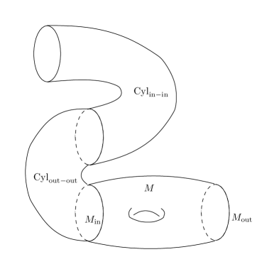
Figure 4. A cobordism with a “tail” of two cylinders (out-out and in-in) attached.

The resulting cobordism $\widetilde{\widetilde{M}}=\mathrm{Cyl}_{\mathrm{in-in}}\cup\mathrm{Cyl}_{\mathrm{out-out}}\cup M$ differs from $M$ by attaching an “in-out” cylinder, thus $Z_{\widetilde{\widetilde{M}}}^{\mathrm{r}}=Z_{M}^{\mathrm{r}}$ by discussion above. On the other hand $Z_{\widetilde{M}}^{\mathrm{r}}$ is independent of cellular decomposition $X$, as is, of course, $Z_{\mathrm{Cyl}_{\mathrm{in-in}}}^{\mathrm{r}}$ (which is also a case of Example 7.14). Therefore $Z_{M}^{\mathrm{r}}=Z_{\widetilde{\widetilde{M}}}^{\mathrm{r}}=\mathrm{Gluing}(Z_{\mathrm{Cyl}_{\mathrm{in-in}}}^{\mathrm{r}},Z_{\widetilde{M}}^{\mathrm{r}})$ is independent on $X$. ($\mathrm{Gluing}(-,-)$ is a schematic notation for the r.h.s. of (105).)

∎

8. Non-abelian cellular $BF$ theory, I: “canonical setting”

The goal of this section is the construction of a “canonical” version of non-abelian cellular $BF$ theory, where the fields are a cochain and a chain of the same CW complex $X$ which is not required to be a manifold. We construct cellular actions (Theorem 8.6) that deform the abelian action, satisfy the BV quantum master equation, are compatible with restrictions to subcomplexes, and on $0$-cells have the canonical form for a $0$-dimensional non-abelian $BF$ theory (this may be viewed as a cellular replacement for the AKSZ construction [1] for topological quantum field theories).

Next, in Section 8.3, we prove that these cellular actions are compatible with elementary collapses (Lemma 8.19) and that the partition function, defined via BV pushforward to cohomology, is a simple-homotopy invariant (Proposition 8.20).

The version of non-abelian cellular $BF$ theory presented in this section is not of Segal type, since one of the fields has “wrong” (covariant) functoriality. On the other hand, we have a version of Mayer-Vietoris gluing formula for the cellular actions (see (vi) of Theorem 8.1).

Throughout this section we adopt the formalism of [27, 28] where the field $B$ of $BF$ theory is treated as covariant (as a cellular chain in discrete setting and as a de Rham current in continuous setting) whereas the field $A$ is contravariant as usual. To reflect this, we denote the fields (and the space of fields) in a different font. Later, in Section 9, we will return to the formalism where both fields are contravariant.

Let $X$ be a finite CW complex (it is not required to be a triangulation of a manifold) and let $\mathfrak{g}$ be a unimodular Lie algebra. We introduce the graded vector space of fields $\mathsf{F}_{X}=C^{\bullet}(X,\mathfrak{g})[1]\oplus C_{\bullet}(X,\mathfrak{g}^{*})[-2]$. As in Section 5.1, it is spanned by the superfields

$$\mathsf{A}_{X}=\sum_{e\subset X}e^{*}\cdot\mathsf{A}_{e} \quad\in\mathrm{Hom}_{1}(\mathsf{F}_{X},C^{\bullet}(X,\mathfrak{g})),$$

$$\mathsf{B}_{X}=\sum_{e\subset X}\mathsf{B}_{e}\cdot e \quad\in\mathrm{Hom}_{-2}(\mathsf{F}_{X},C_{\bullet}(X,\mathfrak{g}^{*}))$$

Here $e^{*},e$ are the standard basis integral cochain and chain, respectively, associated to a cell $e\subset X$; components $\mathsf{A}_{e}$ are $\mathfrak{g}$-valued functions on $\mathsf{F}_{X}$ of degree $1-\dim e$ and components $\mathsf{B}_{e}$ are $\mathfrak{g}^{*}$-valued functions on $\mathcal{F}_{X}$ of degree $-2+\dim e$.

Note that here, unlike in the rest of the paper, the field $\mathsf{B}_{X}$ is a chain of $X$, as opposed to a cochain of $X^{\vee}$ (moreover, in the setup of this subsection, $X^{\vee}$ is meaningless, as $X$ is not required to be a cellular decomposition of a manifold).

The canonical pairing $\langle,\rangle$ between cochains and chains induces a degree $-1$ symplectic form

$$\omega_{X}=\langle\delta\mathsf{B}_{X},\delta\mathsf{A}_{X}\rangle=\sum_{e\subset X}(-1)^{\dim e}\langle\delta\mathsf{B}_{e}\stackrel{{\scriptstyle\wedge}}{{,}}\delta\mathsf{A}_{e}\rangle_{\mathfrak{g}}$$

and a BV Laplacian

$$\Delta_{X}=\left\langle\frac{\partial}{\partial\mathsf{B}_{X}},\frac{\partial}{\partial\mathsf{A}_{X}}\right\rangle=\sum_{e\subset X}(-1)^{\dim e}\left\langle\frac{\partial}{\partial\mathsf{B}_{e}},\frac{\partial}{\partial\mathsf{A}_{e}}\right\rangle_{\mathfrak{g}}$$

on $\mathrm{Fun}(\mathsf{F}_{X})=\widehat{\mathrm{Sym}\,^{\bullet}}\mathsf{F}_{X}^{*}$ (the formal power series in fields). Symbol $\langle,\rangle_{\mathfrak{g}}$ stands for the canonical pairing between $\mathfrak{g}$ and $\mathfrak{g}^{*}$.

In our notation $e\subset X$ stands for an open cell; its closure $\bar{e}=e\cup\partial e\subset X$ is a closed ball (for $X$ a regular CW complex, which we always assume unless stated otherwise) inheriting a structure of CW complex from $X$. Thus, e.g., $\mathsf{A}_{e}$ is a component of the superfield $\mathsf{A}_{X}$, whereas $\mathsf{A}_{\bar{e}}=\sum_{e^{\prime}\subset\bar{e}}(e^{\prime})^{*}\cdot\mathsf{A}_{e^{\prime}}$ is the entire superfield for the subcomplex $\bar{e}\subset X$ containing components of $\mathsf{A}_{X}$ for the cell $e$ itself and cells belonging to the boundary $\partial e$. Likewise, $\partial e\subset X$ is a subcomplex and $\mathsf{A}_{\partial e}=\sum_{e\subset\partial e}(e^{\prime})^{*}\cdot\mathsf{A}_{e^{\prime}}$ is the corresponding $\mathsf{A}$-superfield, and we have $\mathsf{A}_{\bar{e}}=e^{*}\cdot\mathsf{A}_{e}+\mathsf{A}_{\partial e}$.

8.1. Non-abelian $BF$ theory on a simplicial complex, after [27, 28]

Let $X$ be a simplicial complex.

We denote by $\bar{\mathbf{\Delta}}^{N}$ the standard closed simplex of dimension $N\geq 0$, endowed with standard triangulation We view it as a simplicial complex with the top cell the open simplex $\mathbf{\Delta}^{N}$.

Let $\Omega^{\bullet}(X)$ stand for the complex of continuous piecewise polynomial differential forms on (the geometric realization of) $X$. Cochains $C^{\bullet}(X,\mathbb{R})$ can be quasi-isomophically embedded into $\Omega^{\bullet}(X)$ as Whitney forms (continuous piecewise linear forms, linear on every simplex of $X$ w.r.t. its barycentric coordinates), see [36, 11] for details. We denote $\mathsf{i}_{X}:C^{\bullet}(X)\hookrightarrow\Omega^{\bullet}(X)$ the realization of cochains as Whitney forms. This embedding has a natural left inverse, the Poincaré map $\mathsf{p}_{X}:\Omega^{\bullet}(X)\rightarrow C^{\bullet}(X)$ which integrates a form over simplices of $X$, i.e. maps $\alpha\mapsto\sum_{e\subset X}e^{*}\cdot\left(\int_{e}\alpha\right)$. Dupont has constructed an explicit chain homotopy operator $\mathsf{K}_{X}$, contracting $\Omega^{\bullet}(X)$ onto Whitney forms, see [10, 11]. Thus, in the terminology of Section 4, we have a retraction $\Omega^{\bullet}(X)\stackrel{{\scriptstyle(\mathsf{i}_{X},\mathsf{p}_{X},\mathsf{K}_{X})}}{{\rightsquigarrow}}C^{\bullet}(X)$. It is glued (by fiber products) out of building blocks – “standard” retractions for $\bar{\mathbf{\Delta}}^{N}$ for different $N$ (i.e. when restricted to any simplex of $X$, it reduces to a “standard” retraction for a standard simplex).

We will denote by $\ast$ the pushforward of the wedge product of forms (defined piecewise on simplices of $X$) to cochains, $a\ast b:=\mathsf{p}_{X}(\mathsf{i}_{X}(a)\wedge\mathsf{i}_{X}(b))$ – this is a graded-commutative non-associative product on $C^{\bullet}(X)$. Tensoring this operation with the Lie bracket in $\mathfrak{g}$, one gets a bilinear operation $[-\stackrel{{\scriptstyle\ast}}{{,}}-]$ on $C^{\bullet}(X,\mathfrak{g})$ defined by $[x\otimes a\stackrel{{\scriptstyle\ast}}{{,}}y\otimes b]=[x,y]\otimes(a\ast b)$ for $x,y\in\mathfrak{g}$ and $a,b\in C^{\bullet}(X)$.

The following is a reformulation of one of the main results of [28].

Theorem 8.1.

There exists a sequence of elements $\bar{S}_{\mathbf{\Delta}^{N}}\in\mathrm{Fun}(\mathsf{F}_{\bar{\mathbf{\Delta}}^{N}})[[\hbar]]$, for $N=0,1,2,\ldots$, of the form

(106) $$\bar{S}_{\mathbf{\Delta}_{N}}(\mathsf{A}_{\bar{\mathbf{\Delta}}^{N}},\mathsf{B}_{\mathbf{\Delta}^{N}};\hbar)=\\ =\sum_{n=1}^{\infty}\sum_{\Gamma_{0}}\sum_{e_{1},\ldots,e_{n}\subset\bar{\mathbf{\Delta}}^{N}}\frac{1}{|\mathrm{Aut}(\Gamma_{0})|}C^{\mathbf{\Delta}^{N}}_{\Gamma_{0},e_{1},\ldots,e_{n}}\left\langle\mathsf{B}_{\mathbf{\Delta}^{N}},\mathrm{Jacobi}_{\,\Gamma_{0}}(\mathsf{A}_{e_{1}},\ldots,\mathsf{A}_{e_{n}})\right\rangle_{\mathfrak{g}}-\\ -i\hbar\sum_{n=2}^{\infty}\sum_{\Gamma_{1}}\sum_{e_{1},\ldots,e_{n}\subset\bar{\mathbf{\Delta}}^{N}}\frac{1}{|\mathrm{Aut}(\Gamma_{1})|}C^{\mathbf{\Delta}^{N}}_{\Gamma_{1},e_{1},\ldots,e_{n}}\mathrm{Jacobi}_{\,\Gamma_{1}}(\mathsf{A}_{e_{1}},\ldots,\mathsf{A}_{e_{n}})$$

for some values of “structure constants” $C^{\mathbf{\Delta}^{N}}_{\Gamma_{l},e_{0},\ldots,e_{n}}\in\mathbb{R}$, $l=0,1$, such that for any finite simplicial complex $X$ and any unimodular Lie algebra $\mathfrak{g}$ the element

(107) $$S_{X}(\mathsf{A}_{X},\mathsf{B}_{X};\hbar)=\sum_{e\subset X}\bar{S}_{e}(\mathsf{A}_{X}|_{\bar{e}},\mathsf{B}_{e};\hbar)\;\;\in\mathrm{Fun}(\mathsf{F}_{X})[[\hbar]]$$

satisfies

1. the quantum master equation $\Delta_{X}e^{\frac{i}{\hbar}S_{X}}=0$,

2. the property

   (108) $$S_{X}(\mathsf{A}_{X},\mathsf{B}_{X};\hbar)=\langle\mathsf{B}_{X},d\mathsf{A}_{X}\rangle+\frac{1}{2}\langle\mathsf{B}_{X},[\mathsf{A}_{X}\stackrel{{\scriptstyle\ast}}{{,}}\mathsf{A}_{X}]\rangle+\mathcal{R}$$

   with the “error term” $\mathcal{R}\in\widehat{\mathrm{Sym}\,^{\geq 4}}\mathsf{F}_{X}^{*}\oplus\hbar\cdot\widehat{\mathrm{Sym}\,^{\geq 2}}\mathsf{F}_{X}^{*}$.

Here the notations are:

• summation in (106) is over binary rooted trees $\Gamma_{0}$ (oriented towards the root) with $n$ leaves and 1-loop connected 3-valent graphs $\Gamma_{1}$ (with every vertex having two incoming and one outgoing half-edge) with $n$ leaves. Leaves of the graph are decorated by faces $e_{1},\ldots,e_{n}$ (of arbitrary codimension) of $\bar{\mathbf{\Delta}}^{N}$.

• $\mathrm{Jacobi}_{\,\Gamma_{0}}(\mathsf{A}_{e_{1}},\ldots,\mathsf{A}_{e_{n}})$ is the nested Lie bracket in $\mathfrak{g}$, associated to the tree $\Gamma_{0}$, evaluated on elements $\mathsf{A}_{e_{1}},\ldots,\mathsf{A}_{e_{n}}\in\mathfrak{g}$.

• $\mathrm{Jacobi}_{\,\Gamma_{1}}(\mathsf{A}_{e_{1}},\ldots,\mathsf{A}_{e_{n}})$ is the number obtained by cutting the loop of $\Gamma_{1}$ anywhere (resulting in a tree $\widetilde{\Gamma_{1}}$ with $n+1$ leaves, one of which is marked) and taking the trace $\mathrm{tr}_{\mathfrak{g}}\,\mathrm{Jacobi}_{\,\widetilde{\Gamma_{1}}}(\mathsf{A}_{e_{1}},\ldots,\mathsf{A}_{e_{n}},\bullet)$ of the endomorphism of $\mathfrak{g}$ corresponding to the tree.

Remark 8.2.

The proof we present below differs from [27, 28] in its treatment of $S^{(1)}$: here we avoid using regularized infinite-dimensional supertraces over the space of forms $\Omega^{\bullet}(X)$ and instead construct $S^{(1)}$ by purely finite-dimensional methods, using homological perturbation theory. The proof is constructive and, in particular, we can make choices (the only ambiguity in the construction is the choice of induction data in part (iv) in the proof below) that give rational structure constants $C^{\mathbf{\Delta}^{N}}_{\Gamma_{l},e_{1},\ldots,e_{n}}\in\mathbb{Q}$, $l=0,1$.

Sketch of proof.

We split $S_{X}$ as $S_{X}=S_{X}^{(0)}-i\hbar S_{X}^{(1)}$ and treat the components $S_{X}^{(0)}$, $S_{X}^{(1)}$ separately. Likewise, in (106) we split $\bar{S}_{\mathbf{\Delta}^{N}}=\bar{S}_{\mathbf{\Delta}^{N}}^{(0)}-i\hbar\bar{S}_{\mathbf{\Delta}^{N}}^{(1)}$. We break the proof in several steps; we address the construction and properties of $S^{(0)}$ in (i–iii), construction and properties of $S^{(1)}$ for a single simplex in (iv,v), and finally we put everything together in (vi,vii).

1. We construct $S_{X}^{(0)}:=\sum_{\Gamma_{0}}\Phi_{X}^{\Gamma_{0}}(\mathsf{A}_{X},\mathsf{B}_{X})$ where the sum is over binary rooted trees $\Gamma_{0}$ and the contributions $\Phi_{X}^{\Gamma_{0}}(\mathsf{A}_{X},\mathsf{B}_{X})$ are defined as follows, by putting decorations on half-edges of $\Gamma_{0}$ starting from leaves and going inductively to the root.

   • Leaves of $\Gamma_{0}$ are decorated by $\mathsf{i}_{X}(\mathsf{A}_{X})$.

   • In the internal vertices of $\Gamma_{0}$ one calculates the Lie bracket on $\Omega^{\bullet}(X,\mathfrak{g})$ (coming from the wedge product on forms and the Lie bracket in $\mathfrak{g}$) applied to the decorations of the two incoming half-edges and puts the result on the outgoing half-edge.

   • On internal edges one evaluates $-\mathsf{K}_{X}$ applied to the decoration of the in-half-edge and puts the result on the out-half-edge.

   • Finally, we define $\Phi_{X}^{\Gamma_{0}}(\mathsf{A}_{X},\mathsf{B}_{X}):=\frac{1}{|\mathrm{Aut}(\Gamma_{0})|}\langle\mathsf{B}_{X},\mathsf{p}_{X}(\mathfrak{R}_{X}^{\Gamma_{0}}(\mathsf{A}_{X}))\rangle$ where $\mathfrak{R}_{X}^{\Gamma_{0}}(\mathsf{A}_{X})$ is the decoration of the root coming from the assignments above.

   By convention, the contribution of the “trivial tree” (with one leaf and no internal vertices or edges) is $\Phi_{X}^{\mathrm{triv}}:=\langle\mathsf{B}_{X},d\mathsf{A}_{X}\rangle$. We split $S_{X}^{(0)}=S_{X}^{(0),2}+S_{X}^{(0),\geq 3}$ where $S_{X}^{(0),2}$ is another notation for $\Phi_{X}^{\mathrm{triv}}$ and the second term is the contribution of non-trivial trees (the new superscripts $2$, $\geq 3$ denote the degree in fields).

2. It follows from the fact that the data $\Omega^{\bullet}(X)\stackrel{{\scriptstyle(\mathsf{i}_{X},\mathsf{p}_{X},\mathsf{K}_{X})}}{{\rightsquigarrow}}C^{\bullet}(X)$ are assembled from the standard building blocks $\Omega^{\bullet}(\bar{\mathbf{\Delta}}^{N})\stackrel{{\scriptstyle(\mathsf{i}_{\bar{\mathbf{\Delta}}^{N}},\mathsf{p}_{\bar{\mathbf{\Delta}}^{N}},\mathsf{K}_{\bar{\mathbf{\Delta}}^{N}})}}{{\rightsquigarrow}}C^{\bullet}(\bar{\mathbf{\Delta}}^{N})$, and from the factorization $\Omega^{\bullet}(X,\mathfrak{g})=\Omega^{\bullet}(X)\otimes\mathfrak{g}$ into a tensor product of a cdga and a Lie algebra, that $S^{(0)}_{X}$ has the form $S^{(0)}_{X}(\mathsf{A}_{X},\mathsf{B}_{X})=\sum_{e\subset X}\bar{S}^{(0)}_{e}(\mathsf{A}_{X}|_{\bar{e}},\mathsf{B}_{e})$ where $\bar{S}^{(0)}_{\mathbf{\Delta}^{N}}$ satisfies the $\bmod\;\hbar$ part of the ansatz (106).

3. Using Leibniz rule in $\Omega^{\bullet}(X)$ and the identity $d\mathsf{K}_{X}+\mathsf{K}_{X}d=\mathrm{id}-\mathsf{i}_{X}\mathsf{p}_{X}$, one calculates the odd Poisson bracket

   $$\{\Phi_{X}^{\mathrm{triv}},\Phi_{X}^{\Gamma_{0}}\}=\sum_{\mathrm{edges}\;e\mathrm{\;of\;}\Gamma_{0}}\left(-\Phi_{X}^{\Gamma_{0}^{\prime}}\frac{\overleftarrow{\partial}}{\partial\mathsf{A}_{X}}\frac{\overrightarrow{\partial}}{\partial\mathsf{B}_{X}}\Phi_{X}^{\Gamma_{0}^{\prime\prime}}+\Phi_{X}^{\Gamma_{0},e}\right)$$

   where on the r.h.s. we sum over edges $e$ of $\Gamma_{0}$; removing this edge splits $\Gamma_{0}$ into trees $\Gamma_{0}^{\prime}$ and $\Gamma_{0}^{\prime\prime}$. The term $\Phi_{X}^{\Gamma_{0},e}$ is the contribution of $\Gamma_{0}$ with edge $e$ contracted; such contributions cancel when we sum over trees $\Gamma_{0}$ due to the combinatorics of trees and Jacobi identity in $C^{\bullet}(X,\mathfrak{g})$. As a result, summing over $\Gamma_{0}$, we obtain $\{S_{X}^{(0),2},S_{X}^{(0),\geq 3}\}=-\frac{1}{2}\{S_{X}^{(0),\geq 3},S_{X}^{(0),\geq 3}\}$ which together with the obvious identity $\{S_{X}^{(0),2},S_{X}^{(0),2}\}=0$ (a guise of $d^{2}=0$ on cochains) gives the classical master equation

   (109) $$\{S^{(0)}_{X},S^{(0)}_{X}\}=0$$

4. For $N\geq 0$, denote by $Q_{\bar{\mathbf{\Delta}}^{N}}=\{S_{\bar{\mathbf{\Delta}}^{N}}^{(0)},\bullet\}$ the cohomological vector field generated by $S_{\bar{\mathbf{\Delta}}^{N}}^{(0)}$ (the fact that it squares to zero follows from (109) for $X=\bar{\mathbf{\Delta}}^{N}$); it is tangent to $C^{\bullet}(\bar{\mathbf{\Delta}}^{N},\mathfrak{g})[1]\subset\mathsf{F}_{\bar{\mathbf{\Delta}}^{N}}$. Observe that $\Delta S_{\bar{\mathbf{\Delta}}^{N}}^{(0)}\in\mathrm{Fun}_{1}(C^{\bullet}(\bar{\mathbf{\Delta}}^{N},\mathfrak{g})[1])$ is $Q_{\bar{\mathbf{\Delta}}^{N}}$-closed, as follows from (109) and the fact that $\Delta$ is a bi-derivation of $\{\bullet,\bullet\}$. Using homological perturbation theory (Lemma 4.2), one constructs a retraction $\mathrm{Fun}(C^{\bullet}(\bar{\mathbf{\Delta}}^{N},\mathfrak{g})[1]),Q_{\bar{\mathbf{\Delta}}^{N}}\stackrel{{\scriptstyle(\iota,\pi,\kappa)}}{{\rightsquigarrow}}\mathrm{Fun}(\mathfrak{g}[1]),d_{CE}$ where the retract is the Chevalley-Eilenberg cochain complex of the Lie algebra $\mathfrak{g}$. By definition of chain homotopy, one has $Q_{\bar{\mathbf{\Delta}}^{N}}\,\kappa+\kappa\,Q_{\bar{\mathbf{\Delta}}^{N}}=\mathrm{id}-\iota\circ\pi$. Applying both sides of this equation to $\Delta S^{(0)}_{\bar{\mathbf{\Delta}}^{N}}$, and noticing that $\Delta S^{(0)}_{\bar{\mathbf{\Delta}}^{N}}$ is annihilated by $\pi$ (this follows from unimodularity of $\mathfrak{g}$) and is $Q_{\bar{\mathbf{\Delta}}^{N}}$-closed, we obtain $Q_{\bar{\mathbf{\Delta}}^{N}}\kappa\Delta S^{(0)}_{\bar{\mathbf{\Delta}}^{N}}=\Delta S^{(0)}_{\bar{\mathbf{\Delta}}^{N}}$. Therefore, the element $S_{\bar{\mathbf{\Delta}}^{N}}^{(1)}(\mathsf{A}_{\bar{\mathbf{\Delta}}^{N}})\in\mathrm{Fun}_{0}(C^{\bullet}(\bar{\mathbf{\Delta}}^{N},\mathfrak{g})[1])$ constructed as

   (110) $$S_{\bar{\mathbf{\Delta}}^{N}}^{(1)}:=-\kappa\Delta S_{\bar{\mathbf{\Delta}}^{N}}^{(0)}$$

   is a solution of the equation

   (111) $$\Delta S_{\bar{\mathbf{\Delta}}^{N}}^{(0)}+\{S_{\bar{\mathbf{\Delta}}^{N}}^{(0)},S_{\bar{\mathbf{\Delta}}^{N}}^{(1)}\}=0$$

5. One defines

   (112) $$\bar{S}_{\mathbf{\Delta}^{N}}^{(1)}(\mathsf{A}_{\bar{\mathbf{\Delta}}^{N}})=\sum_{e\subset\bar{\mathbf{\Delta}}^{N}}(-1)^{\mathrm{codim}(e)}S_{\bar{e}}^{(1)}(\mathsf{A}_{\bar{\mathbf{\Delta}}^{N}}|_{\bar{e}})$$

   with summands as in (iv) for faces $e$ of $\Delta^{N}$ of arbitrary codimension. One can check from the construction (110), that $\bar{S}_{\mathbf{\Delta}^{N}}^{(1)}$ satisfies the part of ansatz (106) linear in $\hbar$; the property $S_{\bar{\mathbf{\Delta}}^{N}}^{(1)}=\sum_{e\subset\bar{\mathbf{\Delta}}^{N}}\bar{S}^{(1)}_{e}$ is obvious from (112).

6. Assume that a simplicial complex $X$ is given as union of two simplicial subcomplexes $X_{1}$ and $X_{2}$ intersecting over $Y=X_{1}\cap X_{2}$ and assume that the elements $S_{X_{1}}$, $S_{X_{2}}$, $S_{Y}$ as defined by (107) satisfy the quantum master equation on $\mathsf{F}_{X_{1}}$, $\mathsf{F}_{X_{2}}$, $\mathsf{F}_{Y}$ respectively. Then it is straightforward to check that $S_{X}=S_{X_{1}}+S_{X_{2}}-S_{Y}$ (which indeed also satisfies the ansatz (107)) is a solution of the quantum master equation on $\mathsf{F}_{X}$.

7. We break the simplicial complex $X$ into individual simplices $e$; on each of them we have a “building block” solution of the quantum master equation of form $S_{\bar{\mathbf{\Delta}}^{N}}:=S^{(0)}_{\bar{\mathbf{\Delta}}^{N}}-i\hbar S^{(1)}_{\bar{\mathbf{\Delta}}^{N}}$ as constucted in (i) (setting $X=\bar{\mathbf{\Delta}}^{N}$) and (iv), with $N=\dim(e)$. The fact that $S_{\bar{\mathbf{\Delta}}^{N}}$ satisfies the quantum master equation is (109) specialized to $\bar{\mathbf{\Delta}}^{N}$, put together with (111). Then, by (vi), the element $S_{X}$ as defined by (107) satisfies the quantum master equation on $\mathsf{F}_{X}$. Finally, property (b) is obvious from the construction.

∎

Remark 8.3.

Examples of values of structure constants $C$ for a simplex $\mathbf{\Delta}^{N}$ in Theorem 8.1:

$\Gamma,\{e_{i}\}$	$C^{\mathbf{\Delta}^{N}}_{\Gamma,\{e_{i}\}}$
	$\left\{\begin{array}[]{ll}\pm 1&\mathrm{if}\;|e_{1}|=N-1\\ 0&\mathrm{otherwise}\end{array}\right.$
	$\left\{\begin{array}[]{ll}\pm\frac{|e_{1}|!|e_{2}|!}{(N+1)!}&\mathrm{if}\;|e_{1}|+|e_{2}|=N\;\mathrm{and}\;|e_{1}\cap e_{2}|=0\\ 0&\mathrm{otherwise}\end{array}\right.$
	$\left\{\begin{array}[]{ll}\pm\frac{|e_{1}|!|e_{2}|!|e_{3}|!}{(|e_{1}|+|e_{2}|+1)\cdot(N+2)!}&\mathrm{if}\;|e_{1}|+|e_{2}|+|e_{3}|=N+1,\\ &\mathrm{and}\;|e_{1}\cap e_{2}|=0,\\ &\mathrm{and}\;\{|e_{1}\cap e_{3}|,|e_{2}\cap e_{3}|\}=\{0,1\}\\ 0&\mathrm{otherwise}\end{array}\right.$
	$\left\{\begin{array}[]{ll}\frac{(-1)^{N+1}}{(N+1)^{2}(N+2)}&\mathrm{if}\;e_{1}=e_{2}\;\mathrm{and}|e_{1}|=1\\ 0&\mathrm{otherwise}\end{array}\right.$

Here the signs and nonvanishing conditions are formulated in terms of combinatorics and orientations of the $n$-tuple of (arbitrary codimension) faces $e_{1},\ldots,e_{n}$ of $\bar{\mathbf{\Delta}}^{N}$; $|\cdots|$ stands for dimension. The top two graphs correspond, upon summing over the simplices, as in (107), to the cellular differential and the bracket $[\bullet\stackrel{{\scriptstyle*}}{{,}}\bullet]$ (the projected wedge product of forms tensored with the Lie bracket in $\mathfrak{g}$) on cochains and thus to the first two terms of (108). The two bottom graphs give first nontrivial contributions to $\mathcal{R}$ in (108).

Remark 8.4.

Building block (106) for a $0$-simplex $\mathbf{\Delta}^{0}$ is simply $\bar{S}_{\mathbf{\Delta}^{0}}=\frac{1}{2}\left\langle\mathsf{B}_{[0]},[\mathsf{A}_{[0]},\mathsf{A}_{[0]}]\right\rangle$ where we denoted the only cell $[0]:=\mathbf{\Delta}^{0}$ (and we are suppressing the subscript $\mathfrak{g}$ in $\left\langle,\right\rangle$ and $\mathrm{tr}\;$). This corresponds to having a single nonvanishing structure constant $C^{\mathbf{\Delta}^{0}}_{\vbox{\hbox{\includegraphics[scale={0.2}]{tree_2-1_nolabels.pdf}}},[0],[0]}=1$.

The nonvanishing structure constants $C$ of Theorem 8.1 for the $1$-simplex are as follows. We denote the top $1$-cell as $[01]$ and the boundary $0$-cells as $[0]$ and $[1]$.

$\Gamma,\{e_{i}\}$	$C^{\mathbf{\Delta}^{1}}_{\Gamma,\{e_{i}\}}$
	$\left\{\begin{array}[]{ll}(-1)^{n}\frac{B_{n}}{n!}&\mathrm{if}\;\{e_{0},e_{1}\}=\{[1],[01]\},\;e_{2}=\cdots=e_{n}=[01]\\ -\frac{B_{n}}{n!}&\mathrm{if}\;\{e_{0},e_{1}\}=\{[0],[01]\},\;e_{2}=\cdots=e_{n}=[01]\\ 0&\mathrm{otherwise}\end{array}\right.$
	$\left\{\begin{array}[]{ll}\frac{B_{n}}{n!}&\mathrm{if}\;e_{1}=\cdots=e_{n}=[01]\\ 0&\mathrm{otherwise}\end{array}\right.$

Here $B_{n}$ are the Bernoulli numbers, $B_{0}=1,\,B_{1}=-\frac{1}{2},\,B_{2}=\frac{1}{6},\,B_{3}=0,B_{4}=-\frac{1}{30},\ldots$ In particular, the building block (106) for $\mathbf{\Delta}^{1}$ is

(113) $$\bar{S}_{\mathbf{\Delta}^{1}}=\left\langle\mathsf{B}_{[01]},\mathsf{A}_{[1]}-\mathsf{A}_{[0]}\right\rangle+\frac{1}{2}\left\langle\mathsf{B}_{[01]},[\mathsf{A}_{[01]},\mathsf{A}_{[0]}+\mathsf{A}_{[1]}]\right\rangle-\frac{1}{12}\left\langle\mathsf{B}_{[01]},[\mathsf{A}_{[01]},[\mathsf{A}_{[01]},\mathsf{A}_{[1]}-\mathsf{A}_{[0]}]]\right\rangle+\cdots-\\ -i\hbar\left(\frac{1}{24}\mathrm{tr}\,[\mathsf{A}_{[01]},[\mathsf{A}_{[01]},\bullet]]+\cdots\right)=\\ =\left\langle\mathsf{B}_{[01]},\frac{1}{2}\left[\mathsf{A}_{[01]},\mathsf{A}_{[0]}+\mathsf{A}_{[1]}\right]+\mathbb{F}(\mathrm{ad}_{\mathsf{A}_{[01]}})\circ(\mathsf{A}_{[1]}-\mathsf{A}_{[0]})\right\rangle-i\hbar\;\mathrm{tr}\log\mathbb{G}(\mathrm{ad}_{\mathsf{A}_{[01]}})$$

where we introduced the two functions

(114) $$\mathbb{F}(x)=\frac{x}{2}\coth\frac{x}{2},\qquad\mathbb{G}(x)=\frac{2}{x}\sinh\frac{x}{2}$$

Remark 8.5.

We have required $X$ to be a simplicial complex rather than a general $CW$ complex because for the Theorem 8.1 we need retractions $\Omega^{\bullet}(\bar{e})\stackrel{{\scriptstyle}}{{\rightsquigarrow}}C^{\bullet}(\bar{e})$ for cells $e$ of $X$, compatible with restriction to cells of $\partial e$ (if we want “standard building blocks” as in Theorem 8.1, we should also require that the retraction depends only on the combinatorial type of $\bar{e}$ and is compatible with combinatorial symmetries of the cell). In the case of simplices, such retractions are provided by Whitney forms and Dupont’s chain homotopy operator (whereas Poincaré map works for cells of any type). More generally, we can allow $X$ to be a prismatic complex, with cells $e=\sigma_{1}\times\cdots\times\sigma_{r}$ being prisms – products of simplices (of arbitrary dimension). The respective retraction $\Omega^{\bullet}(\bar{e})\stackrel{{\scriptstyle}}{{\rightsquigarrow}}C^{\bullet}(\bar{e})$ is constructed from Whitney/Dupont retractions for simplices by the tensor product construction of Section 4.2 (whenever we have several simplices of same dimension in $e$, we average over the order in which we contract the factors, in order to have the retraction compatible with the symmetries of the prism). The special case when the prisms are cubes (products of 1-simplices) was considered in detail in [28]. As a result, one can allow $X$ in Theorem 8.1 to be a prismatic complex; the building blocks $\bar{S}_{e}$ then depend on the combinatorial type of the prism $e$ (dimensions of the simplex factors) and the structure constants $C^{e}_{\Gamma_{0},e_{1},\ldots,e_{n}}$, $C^{e}_{\Gamma_{1},e_{1},\ldots,e_{n}}$ depend on the combinatorics of an $n$-tuple of faces of the prism $e$. In Section 8.2 we will construct a further generalization of Theorem 8.1 to general regular CW complexes.

8.2. Case of general CW complexes

One can extend Theorem 8.1 to a general regular CW complex, with cells not required to be simplices or prisms.

Theorem 8.6.

Let $X$ be a finite regular CW complex and $\mathfrak{g}$ be a unimodular Lie algebra. Then to every cell $e\subset X$ one can associate an element (a local building block) $\bar{S}_{e}\in\mathrm{Fun}(\mathsf{F}_{\bar{e}})[[\hbar]]$ of the form

(115) $$\bar{S}_{e}(\mathsf{A}_{\bar{e}},\mathsf{B}_{e};\hbar)=\\ =\sum_{n=1}^{\infty}\sum_{\Gamma_{0}}\sum_{e_{1},\ldots,e_{n}\subset\bar{e}}\frac{1}{|\mathrm{Aut}(\Gamma_{0})|}C^{e}_{\Gamma_{0},e_{1},\ldots,e_{n}}\left\langle\mathsf{B}_{e},\mathrm{Jacobi}_{\,\Gamma_{0}}(\mathsf{A}_{e_{1}},\ldots,\mathsf{A}_{e_{n}})\right\rangle_{\mathfrak{g}}-\\ -i\hbar\sum_{n=2}^{\infty}\sum_{\Gamma_{1}}\sum_{e_{1},\ldots,e_{n}\subset\bar{e}}\frac{1}{|\mathrm{Aut}(\Gamma_{1})|}C^{e}_{\Gamma_{1},e_{1},\ldots,e_{n}}\mathrm{Jacobi}_{\,\Gamma_{1}}(\mathsf{A}_{e_{1}},\ldots,\mathsf{A}_{e_{n}})$$

with some real coefficients $C^{e}_{\Gamma_{l},e_{1},\ldots,e_{n}}\in\mathbb{R}$ for $l=0,1$, in such a way that the element (the cellular action)

(116) $$S_{X}(\mathsf{A}_{X},\mathsf{B}_{X};\hbar)=\sum_{e\subset X}\bar{S}_{e}(\mathsf{A}_{X}|_{\bar{e}},\mathsf{B}_{e};\hbar)\;\;\in\mathrm{Fun}(\mathsf{F}_{X})[[\hbar]]$$

satisfies the quantum master equation $\Delta_{X}e^{\frac{i}{\hbar}S_{X}}=0$ and the following conditions:

1. the property

   (117) $$S_{X}(\mathsf{A}_{X},\mathsf{B}_{X};\hbar)=\left\langle\mathsf{B}_{X},d\mathsf{A}_{X}\right\rangle+\mathfrak{r}$$

   with $\mathfrak{r}\in\widehat{\mathrm{Sym}\,^{\geq 3}}\mathsf{F}_{X}^{*}\oplus\hbar\cdot\widehat{\mathrm{Sym}\,^{\geq 2}}\mathsf{F}^{*}_{X}$,

2. for $e$ any $0$-cell of $X$, one has

   (118) $$\bar{S}_{e}=\left\langle\mathsf{B}_{e},\frac{1}{2}[\mathsf{A}_{e},\mathsf{A}_{e}]\right\rangle_{\mathfrak{g}}$$

3. For $Y\subset X$ any subcomplex, $S_{Y}(\mathsf{A}_{Y},\mathsf{B}_{Y};\hbar):=\sum_{e\subset Y}\bar{S}_{e}\;\in\mathrm{Fun}(\mathsf{F}_{Y})[[\hbar]]$ satisfies the quantum master equation on $\mathsf{F}_{Y}$.

Proof.

Choose an ordering of the cells $e_{1},\ldots,e_{N}$ of $X$ in such a way that $\dim e_{1}\leq\cdots\leq\dim e_{N}$. Then $X$ admits an increasing filtration by CW subcomplexes

(119) $$X_{1}\subset\cdots\subset X_{N-1}\subset X_{N}=X$$

with $X_{k}:=\cup_{i\leq k}e_{i}$. Then $X_{k}=X_{k-1}\cup e_{k}$. That is, $X_{k}$ is $X_{k-1}$ with a single new cell $e_{k}$ adjoined; its boundary $\partial e_{k}$ lies entirely in $X_{k-1}$.

Proceeding by induction in $k$, assume that a solution $S_{X_{k-1}}$ of the QME on $\mathsf{F}_{X_{k-1}}$ is constructed and we want to extend it to $\mathsf{F}_{X_{k}}=\mathsf{F}_{X_{k-1}}[\mathsf{A}_{e},\mathsf{B}_{e}]$ (we temporarily denote $e:=e_{k}$). Denote $n=\dim e$. First, we look for a solution of the classical master equation $S^{(0)}_{X_{k}}$ of the following form

(120) $$S^{(0)}_{X_{k}}=S^{(0)}_{X_{k-1}}+\underbrace{\sum_{j\geq 1}\left\langle\mathsf{B}_{e},\sigma_{j}(\mathsf{A}_{e},\mathsf{A}_{\partial e})\right\rangle}_{\bar{S}^{(0)}_{e}}$$

where $\sigma_{j}$ is of polynomial degree $j$ in $\mathsf{A}$-variables (we call this polynomial degree weight to distinguish it from other gradings). We assume $n\geq 1$ (otherwise we simply set $\bar{S}_{e}=\left\langle\mathsf{B}_{e},\frac{1}{2}[\mathsf{A}_{e},\mathsf{A}_{e}]\right\rangle$ as prescribed by (b)).

We denote by

$$d_{\partial e\rightarrow e}=e^{*}\cdot\mathsf{d}_{\partial e\rightarrow e}:\quad C^{n-1}(\partial e)\;\;\rightarrow\;\;C^{n}(\bar{e},\partial e)=\mathrm{Span}(e^{*})$$

the component of the cellular coboundary operator on $X_{k}$ proportional to $e^{*}$ (and $\mathsf{d}_{\partial e\rightarrow e}:C^{n-1}(\partial e)\rightarrow\mathbb{R}$ picks the coefficient of $e^{*}$). Thus, the cellular coboundary operator on $C^{\bullet}(\bar{e})$ splits as $d_{\bar{e}}=d_{\partial e}+d_{\partial e\rightarrow e}$ with $d_{\partial e}$ the cellular coboundary operator on $C^{\bullet}(\partial e)$. Let us choose some induction data

(121) $$C^{\bullet}(\bar{e}),d_{\bar{e}}\stackrel{{\scriptstyle(i,p,K)}}{{\rightsquigarrow}}H^{\bullet}(\bar{e})=\left\{\begin{array}[]{ll}\mathbb{R},&\bullet=0\\ 0,&\bullet\neq 0\end{array}\right.$$

Consider the space

$$\mathcal{E}^{j}:=\mathrm{Sym}\,^{j}(C^{\bullet}(\bar{e},\mathfrak{g})[1])^{*}\qquad\ni f(\mathsf{A}_{e},\mathsf{A}|_{\partial e})$$

The operator $d_{\partial e\rightarrow e}$ lifts to a weight zero operator

$$D=(-1)^{n}\left\langle\mathsf{d}_{\partial e\rightarrow e}\;\mathsf{A}_{\partial e},\frac{\partial}{\partial\mathsf{A}_{e}}\right\rangle:\quad\mathcal{E}^{\bullet}\rightarrow\mathcal{E}^{\bullet}$$

Denote by $Q_{\partial e}$ the differential on $\mathrm{Sym}\,(C^{\bullet}(\partial e,\mathfrak{g})[1])$ induced by $\{S_{X_{k-1}}^{(0)},\bullet\}$; it extends (via $Q_{\partial e}\mathsf{A}_{e}=0$) to $\mathcal{E}^{\bullet}$. We split $Q_{\partial e}$ according to weight as $Q_{\partial e}=Q_{\partial e}^{0}+Q_{\partial e}^{1}+\cdots$. In particular, $Q^{0}_{\partial e}+D$ is simply the lift of the cellular coboundary operator $d_{\bar{e}}$ to $\mathcal{E}^{\bullet}$. Thus, using the construction (19), one produces, out of the triple $(i,p,K)$ chosen above, the induction data

(122) $$\mathcal{E}^{\bullet},Q^{0}_{\partial e}+D\stackrel{{\scriptstyle(i_{\mathcal{E}},p_{\mathcal{E}},K_{\mathcal{E}})}}{{\rightsquigarrow}}H^{\bullet}(\mathcal{E})\cong\mathrm{Sym}\,^{\bullet}(\mathfrak{g}[1])^{*}$$

Note that $i$ in (121) is canonical: it has to represent $H^{0}(\bar{e})$ by constant $0$-cochains; thus $p_{\mathcal{E}}=i^{*}$ is also canonical and is given by evaluation on constant $0$-cochains.

We set in (120) the “initial condition” $\sigma_{1}:=\mathsf{d}_{\partial e\rightarrow e}\,\mathsf{A}_{\partial e}$, which is forced by (117). The classical master equation $\{S^{(0)}_{X_{k}},S^{(0)}_{X_{k}}\}=0$ is equivalent to a sequence of equations for the functions $\sigma_{j}$ for $j\geq 2$:

(123) $$(D+Q^{0}_{\partial e})\sigma_{j}=-\sum_{i=1}^{j-1}Q^{i}_{\partial e}\sigma_{j-i}-(-1)^{n}\sum_{i=2}^{j-1}\left\langle\sigma_{j+1-i},\frac{\partial}{\partial\mathsf{A}_{e}}\right\rangle\sigma_{i}$$

Note that the r.h.s. of (123) depends only on $\sigma_{1},\ldots,\sigma_{j-1}$. We solve (123), as an equation for $\sigma_{j}\in\mathfrak{g}\otimes\mathcal{E}^{j}$, by induction in $j$. The r.h.s. is $(D+Q^{0}_{\partial e})$-closed and is annihilated by $p_{\mathcal{E}}$. Therefore, it is exact, and one can construct the primitive as

$$\sigma_{j}:=K_{\mathcal{E}}\left(\mbox{r.h.s. of }(\ref{cellBF CME induction})\right)$$

Thus we have constructed a solution of the classical master equation (120) on $X_{k}$ by extension of the known one (by induction hypothesis) on $X_{k-1}$.

Next, we want to construct $S^{(1)}_{X_{k}}=S^{(1)}_{X_{k-1}}+\bar{S}^{(1)}_{e}(\mathsf{A}_{e},\mathsf{A}_{\partial e})$ in such a way that $S_{X_{k}}=S^{(0)}_{X_{k}}-i\hbar\,S^{(1)}_{X_{k}}$ satisfies the quantum master equation; we assume that $S^{(1)}_{X_{k-1}}$ is already constructed. We use the strategy of (iv) of the proof of Theorem 8.1: the QME can be written as

(124) $$Q_{\bar{e}}S^{(1)}_{\bar{e}}=-\Delta S^{(0)}_{\bar{e}}$$

where $Q_{\bar{e}}=Q_{\partial e}+D+(-1)^{n}\sum_{j\geq 2}\left\langle\sigma_{j},\frac{\partial}{\partial\mathsf{A}_{e}}\right\rangle$ is the differential on $\mathcal{E}^{\bullet}$ induced by $\{S^{(0)}_{X_{k}},\bullet\}$ and $S^{(0,1)}_{\bar{e}}:=\sum_{e^{\prime}\subset e}\bar{S}^{(0,1)}_{e^{\prime}}$. We deform the induction data (122), using Lemma 4.2, to

$$\mathcal{E}^{\bullet},Q_{\bar{e}}\stackrel{{\scriptstyle(\widetilde{i}_{\mathcal{E}},\widetilde{p}_{\mathcal{E}},\widetilde{K}_{\mathcal{E}})}}{{\rightsquigarrow}}\mathrm{Sym}\,^{\bullet}(\mathfrak{g}[1])^{*},d_{CE}$$

The r.h.s. of (124) is $Q_{\bar{e}}$-closed, as follows from the classical master equation, and is annihilated by $\widetilde{p}_{\mathcal{E}}$ (from unimodularity of $\mathfrak{g}$), thus we construct a solution of (124) as $S^{(1)}_{\bar{e}}:=-\widetilde{K}_{\mathcal{E}}\Delta S^{(0)}_{\bar{e}}$ and set

$$\bar{S}^{(1)}_{e}:=S^{(1)}_{\bar{e}}-\sum_{e^{\prime}\subset\partial e}\bar{S}^{(1)}_{e^{\prime}}$$

This finishes the construction of a solution of the quantum master equation on $X_{k}$ of the form $S_{X_{k}}=\sum_{i\leq k}\bar{S}_{e_{i}}$ with $\bar{S}_{e_{i}}=\bar{S}^{(0)}_{e_{i}}-i\hbar\,\bar{S}^{(1)}_{e_{i}}$; taking $k=N$ we obtain the statement of the Theorem.

Property (c) follows from the possibility to choose the ordering of cells $e_{1},\ldots,e_{N}$ differently (preserving the nondecreasing dimension property) while preserving the choice of induction data (121) for the cells. Each $Y\subset X$ arises as $X_{k}$ for some ordering of cells and some $k$, which implies the QME on $Y$. ∎

Lemma 8.7.

Cellular action $S_{X}$ of the Theorem 8.6 is well-defined up to a canonical BV transformation. More precisely, let $S_{X}$ and $S^{\prime}_{X}$ be two cellular actions fulfilling the conditions of Theorem 8.6 – the quantum master equation, the ansatz (116,115) and properties (a)–(c). Then one can construct a family $S_{X,t}\in\mathrm{Fun}_{0}(\mathsf{F}_{X})[[\hbar]]$ of solutions of QME for $t\in[0,1]$ together with a generator $R_{X,t}\in\mathrm{Fun}_{-1}(\mathsf{F}_{X})[[\hbar]]$ such that

1. $S_{X,0}=S_{X}$, $S_{X,1}=S^{\prime}_{X}$,

2. $\frac{\partial}{\partial t}S_{X,t}=\{S_{X,t},R_{X,t}\}-i\hbar\Delta R_{X,t}$,

3. both $S_{X,t}$ and $R_{X,t}$ satisfy the ansatz (116,115), with $t$-dependent structure constants $C^{S,e}_{\Gamma,e_{1},\ldots,e_{n}}(t)$, $C^{R,e}_{\Gamma,e_{1},\ldots,e_{n}}(t)$ for the action $S_{X,t}$ and the generator of infinitesimal canonical transformation $R_{X,t}$. Moreover, the trivial tree $\Gamma_{0}^{\mathrm{triv}}$ with a single leaf and no internal vertices has coefficient $C^{R,e}_{\Gamma_{0}^{\mathrm{triv}},e_{1}}=0$).

Proof.

Consider the filtration (119). We proceed by induction in $X_{k}$: assuming that the Lemma holds for $X_{k-1}$, we aim to prove it for $X_{k}$. (Note that the Lemma holds trivially for $X_{1}$, since $S_{X_{1}}$ is fixed uniquely by (b) of Theorem 8.6.) Set $S_{X_{k}}:=\sum_{l=1}^{k}\bar{S}_{e_{l}}$, $S^{\prime}_{X_{k}}:=\sum_{l=1}^{k}\bar{S}^{\prime}_{e_{l}}$. By induction hypothesis, cellular actions $S_{X_{k-1}}$ and $S^{\prime}_{X_{k-1}}$ (defined as above, omitting the $k$-th term in the sums) are connected by a canonical BV transformation, which we denote schematically by $\mathcal{R}_{X_{k-1}}$, i.e. $S^{\prime}_{X_{k-1}}=\mathcal{R}_{X_{k-1}}\circ S_{X_{k-1}}$.

Define

(125) $$S^{\prime\prime}_{X_{k}}:=\mathcal{R}_{X_{k-1}}^{-1}S^{\prime}_{X_{k}}$$

We have then $S_{X_{k}}=S_{X_{k-1}}+\bar{S}_{e}$ and $S^{\prime\prime}_{X_{k}}=S_{X_{k-1}}+\bar{S}^{\prime\prime}_{e}$ (for some $\bar{S}^{\prime\prime}_{e}(\mathsf{A}_{\bar{e}},\mathsf{B}_{e};\hbar)$ satisfying the ansatz (115)). We can connect $S_{X_{k}}$ and $S^{\prime\prime}_{X_{k}}$ by a path of solutions of QME on $\mathsf{F}_{X_{k}}$ of the form $S_{X_{k},t}=S_{X_{k-1}}+\bar{S}_{e,t}$ for $t\in[0,1]$, with $\bar{S}_{e,t}=\bar{S}_{e,t}^{(0)}-i\hbar\,\bar{S}_{e,t}^{(1)}=\left\langle\mathsf{B}_{e},\sigma_{t}(\mathsf{A}_{\bar{e}})\right\rangle-i\hbar\,\rho_{t}(\mathsf{A}_{\bar{e}})$ for some $t$-dependent functions $\sigma_{t}\in\mathfrak{g}\otimes\mathcal{E}^{\geq 2}$, $\rho_{t}\in\mathcal{E}^{\geq 2}$ of $\mathsf{A}$-variables of weight $\geq 2$. (We are borrowing the notations of the proof of Theorem 8.6, in particular $e:=e_{k}$.)

Differentiating QME for $S_{X_{t}}$ in $t$, we obtain

(126) $$\{S_{X_{k},t}^{(0)},\dot{\bar{S}}_{e,t}^{(0)}\} = 0$$

(127) $$\{S^{(1)}_{X_{k},t},\dot{\bar{S}}_{e,t}^{(0)}\}+\{S^{(0)}_{X_{k},t},\dot{\bar{S}}_{e,t}^{(1)}\}+\Delta\dot{\bar{S}}_{e,t}^{(0)} = 0$$

where the dot stands for the derivative in $t$.

Observe that:

1. The cohomology of the differential $\{\left\langle\mathsf{B}_{X_{k}},d\mathsf{A}_{X_{k}}\right\rangle,\bullet\}$ on the subcomplex $\Xi^{(0)}:=\{\left\langle\mathsf{B}_{e},f(\mathsf{A}_{\bar{e}})\right\rangle\,|\,f\in\mathfrak{g}\otimes\mathcal{E}^{\geq 2}\}\subset\mathrm{Fun}(\mathsf{F}_{X_{k}})$ vanishes in internal degree zero. This implies, by homological perturbation theory, that degree zero cohomology of $\{S^{(0)}_{X_{k},t},\bullet\}$ on $\Xi^{(0)}$ vanishes as well.

2. By a similar argument, degree zero cohomology of $\{S^{(0)}_{X_{k},t},\bullet\}$ on $\Xi^{(1)}:=\{g(\mathsf{A}_{\bar{e}})\in\mathcal{E}^{\geq 2}\}\subset\mathrm{Fun}(\mathsf{F}_{X_{k}})$ also vanishes.

Thus, by (126) and (a), we have $\dot{\bar{S}}_{e,t}^{(0)}=\{S_{X_{k},t}^{(0)},r^{(0)}_{e,t}\}$ for some degree $-1$ element $r^{(0)}_{e,t}\in\Xi^{(0)}$. Substituting this into (127), we obtain, using Jacobi identity for $\{,\}$ and the QME on $S_{X_{k},t}$, that $\left\{S^{(0)}_{X_{k},t},\dot{\bar{S}}_{e,t}^{(1)}-\{S^{(1)}_{X_{k},t},r^{(0)}_{e,t}\}-\Delta r^{(0)}_{e,t}\right\}=0$. This implies, by (b), that $\dot{\bar{S}}_{e,t}^{(1)}=\{S^{(1)}_{X_{k},t},r^{(0)}_{e,t}\}+\Delta r^{(0)}_{e,t}+\{S^{(0)}_{X_{k},t},r^{(1)}_{e,t}\}$ for some degree $-1$ element $r^{(1)}_{e,t}\in\Xi^{(1)}$. Thus we have proven that

(128) $$\dot{S}_{X_{k},t}=\{S_{X_{k},t},r_{e,t}\}-i\hbar\,\Delta r_{e,t}$$

with the generator $r_{e,t}=r^{(0)}_{e,t}-i\hbar\,r^{(1)}_{e,t}\in\,\Xi^{(0)}-i\hbar\,\Xi^{(1)}$. One can use homological perturbation theory to construct an explicit chain contractions of $\left(\Xi^{(0)},\{S^{(0)}_{X_{k},t},\bullet\}\right)$ and $\left(\Xi^{(1)},\{S^{(0)}_{X_{k},t},\bullet\}\right)$ and use them to construct $r^{(0)}_{e,t}$, $r^{(1)}_{e,t}$. By inspection of the construction, the resulting generator $r_{e,t}$ satisfies the ansatz (115) for some $t$-dependent structure constants $C^{r,e}_{\Gamma,e_{1},\ldots,e_{n}}(t)$.

Combining (128) and (125), we obtain that $S_{X_{k}}$ and $S^{\prime}_{X_{k}}$ can be connected by a canonical transformation (ii) with generator

$$R_{X_{k},t}=\left\{\begin{array}[]{ll}2r_{e,2t},&t\in[0,\frac{1}{2})\\ 2R_{X_{k-1},2t-1},&t\in[\frac{1}{2},1]\end{array}\right.$$

This proves the induction step $X_{k-1}\rightarrow X_{k}$. ∎

Remark 8.8.

One can put together $S_{X,t}$ and $R_{X,t}$ of Lemma 8.7 into a single non-homogeneous differential form on the interval,

$$\widetilde{S}_{X}:=S_{X,t}+dt\cdot R_{X,t}\in\Omega^{\bullet}([0,1])\widehat{\otimes}\mathrm{Fun}(\mathsf{F}_{X})[[\hbar]]$$

Then the quantum master equation on $S_{X,t}$ together with (ii) can be packaged as an extended quantum master equation for $\tilde{S}_{X}$,

$$(d_{t}-i\hbar\,\Delta)\,e^{\frac{i}{\hbar}\widetilde{S}_{X}}=0$$

where $d_{t}=dt\cdot\frac{\partial}{\partial t}$ – the de Rham differential in $t$. By the Lemma, $\widetilde{S}_{X}$ satisfies the ansatz (116,115) with structure constants $C$ taking values in $\Omega^{\bullet}([0,1])$.

Remark 8.9.

The building block (115) of the cellular action is defined uniquely for $\dim e=0$ (fixed by (118)) and for $\dim e=1$ (as follows from Lemma 8.7: for degree reasons, the generator of the canonical transformation has to vanish; $\bar{S}_{e}$ in this case is given by (113)). For cells of dimension $\geq 2$, $\bar{S}_{e}$ is not uniquely defined.

Remark 8.10.

A different approach to the proof of Theorem 8.6 is to fix a simplicial refinement $W$ of $X$ (i.e. cells of $X$ are triangulated in $W$). Then, proceeding again by induction in $X_{k}$, as in (119), one constructs $S_{X_{k}}$ as a BV pushforward of $S_{W_{k}}$, as constructed in Theorem 8.1 ($W_{k}$ here is the restriction of $W$ to $X_{k}$), using a choice of gauge-fixing compatible with one for the BV pushforward $W_{k-1}\rightarrow X_{k-1}$ used in the previous step and involving a choice of induction data for relative cochains $C^{\bullet}(W|_{e_{k}},\partial e_{k})\stackrel{{\scriptstyle}}{{\rightsquigarrow}}C^{\bullet}(\bar{e}_{k},\partial e_{k})$.

Remark 8.11 (Standard building blocks for cells).

Assume that we have fixed some “standard” choice of the induction data (121) for all possible regular CW decompositions $\bar{e}$ of a closed $n$-ball with single top cell, considered up to homeomorphisms, for $n\geq 1$. Denote this collection of choices $\theta$. Then, by the construction of Theorem 8.6, we have a “standard building block” $\bar{S}_{e}^{\theta}$ satisfying ansatz (115) for any possible combinatorics of $\bar{e}$. For any finite regular CW complex $X$, we then have a “standard” cellular action $S^{\theta}_{X}=\sum_{e\subset X}\bar{S}^{\theta}_{e}$ satisfying the quantum master equation and properties (a–c) of Theorem 8.6. In particular, we can choose $\theta$ on simplices (and, more generally, on prisms, see Remark 8.5) to give the building blocks (106) of Theorem 8.1, coming from Whitney forms/Dupont’s chain homotopy.

Remark 8.12 (Rationality).

We can choose the induction data (121) for cells to be rational, i.e. to factor through induction data $C^{\bullet}(\bar{e},\mathbb{Q})\stackrel{{\scriptstyle(i_{\mathbb{Q}},p_{\mathbb{Q}},K_{\mathbb{Q}})}}{{\rightsquigarrow}}H^{\bullet}(\bar{e},\mathbb{Q})$. Then, by inspection of the proof of Theorem 8.6, all the structure constants of the cellular action – coefficients $C^{e}_{\Gamma_{0},e_{1},\ldots,e_{n}}$, $C^{e}_{\Gamma_{1},e_{1},\ldots,e_{n}}$ in (115) – are rational as well.

8.2.1. Cellular $BF$ action as a “generating function” of a unimodular $L_{\infty}$ algebra on cochains

Definition 8.13.

A unimodular $L_{\infty}$ algebra is a graded vector space $V^{\bullet}$ endowed with two sequences of skew-symmetric multilinear operations,

• classical operations $l_{n}:\,\wedge^{n}V\rightarrow V$ for $n\geq 1$ of degree $2-n$ and

• quantum operations $q_{n}:\,\wedge^{n}V\rightarrow\mathbb{R}$ for $n\geq 1$ of degree $-n$,

such that the following two sequences of identities hold: homotopy Jacobi identities

(129) $$\sum_{\sigma\in\Sigma_{n}}\sum_{r+s=n}\pm\frac{1}{r!s!}\,l_{r+1}(x_{\sigma_{1}},\ldots,x_{\sigma_{r}},l_{s}(x_{\sigma_{r+1}},\ldots,\sigma_{n}))=0$$

and homotopy unimodularity relations

(130) $$\sum_{\sigma\in\Sigma_{n}}\left(\pm\frac{1}{n!}\,\mathrm{Str}_{V}\;l_{n+1}(x_{\sigma_{1}},\ldots,x_{\sigma_{n}},\bullet)+\sum_{r+s=n}\pm\frac{1}{r!s!}\,q_{r+1}(x_{\sigma_{1}},\ldots,x_{\sigma_{r}},l_{s}(x_{\sigma_{r+1}},\ldots,x_{\sigma_{n}}))\right)=0$$

Here $x_{1},\ldots,x_{n}$ is an $n$-tuple of elements of $V$ and $\sigma$ runs over permutations of this $n$-tuple; $\pm$ are the Koszul signs.

Definition 8.14 ([28]).

For $V^{\bullet}$ a graded vector space, consider the odd-symplectic space $\mathsf{F}=V[1]\oplus V^{*}[-2]$. We say that an element $f\in\mathrm{Fun}(\mathsf{F})[[\hbar]]$ satisfies the “$BF_{\infty}$ ansatz” if

(131) $$f=\left\langle\mathsf{B},\alpha(\mathsf{A})\right\rangle-i\hbar\beta(\mathsf{A})$$

where $\mathsf{A}\in\mathrm{Hom}_{1}(\mathsf{F},V)$, $\mathsf{B}\in\mathrm{Hom}_{-2}(\mathsf{F},V^{*})$ are the superfields (projections to summands of $\mathsf{F}$ composed with shifted identity map) and $\alpha(\mathsf{A})\in\widehat{\mathrm{Sym}\,^{\geq 1}}(V[1])\otimes V^{*}$, $\beta(\mathsf{A})\in\widehat{\mathrm{Sym}\,^{\geq 1}}(V[1])$ arbitrary elements.

We have the following properties (see [28] for details and proofs):

1. If $f$ and $g$ satisfy the $BF_{\infty}$ ansatz then $\{f,g\}$ and $\Delta f$ also satisfy it.

2. If $S$ satisfies the $BF_{\infty}$ ansatz and is of internal degree zero, then one can write

   (132) $$S(\mathsf{A},\mathsf{B};\hbar)=\sum_{n\geq 1}\frac{1}{n!}\langle\mathsf{B},l_{n}(\underbrace{\mathsf{A},\ldots,\mathsf{A}}_{n})\rangle-i\hbar\sum_{n\geq 1}\frac{1}{n!}q_{n}(\underbrace{\mathsf{A},\ldots,\mathsf{A}}_{n})$$

   where $l_{n}:\,\wedge^{n}V\rightarrow V$ and $q_{n}:\,\wedge^{n}V\rightarrow\mathbb{R}$ are certain multilinear operations on $V$. They endow $V$ with the structure of a unimodular $L_{\infty}$ algebra, as in Definition 49. Relations (129,130) can be conveniently written in terms of the superfield $\mathsf{A}_{X}$ as

   $$\sum_{r+s=n}\frac{1}{r!s!}\,l_{r+1}(\underbrace{\mathsf{A},\ldots,\mathsf{A}}_{r},l_{s}(\underbrace{\mathsf{A},\ldots,\mathsf{A}}_{s}))=0,$$

   $$\frac{1}{n!}\,\mathrm{Str}\;l_{n+1}(\underbrace{\mathsf{A},\ldots,\mathsf{A}}_{n},\bullet)+\sum_{r+s=n}\frac{1}{r!s!}\,q_{r+1}(\underbrace{\mathsf{A},\ldots,\mathsf{A}}_{r},l_{s}(\underbrace{\mathsf{A},\ldots,\mathsf{A}}_{s}))=0$$

   and are equivalent to the quantum master equation satisfied by $S$.

3. If $S_{t}$, for $t\in[0,1]$, is a family of solutions of the QME satisfying the $BF_{\infty}$ ansatz such that $S_{t}$ for different $t$ are related by a canonical BV transformation

   (133) $$\frac{\partial}{\partial t}\,S_{t}=\{S_{t},R_{t}\}-i\hbar\,R_{t}$$

   then the degree $-1$ generator $R_{t}$ has to satisfy the $BF_{\infty}$ ansatz as well.

4. One can introduce a natural notion of equivalence of unimodular $L_{\infty}$ structures on $V$: two structures $\{l_{n},q_{n}\}$, $\{l^{\prime}_{n},q^{\prime}_{n}\}$ are called equivalent if the corresponding solutions (132) of QME on $\mathsf{F}$ can be related by a canonical BV transformation (133).

In particular, for $V=C^{\bullet}(X,\mathfrak{g})$, the action $S_{X}$ constructed in Theorem 8.6 can be expanded as

(134) $$S_{X}(\mathsf{A}_{X},\mathsf{B}_{X};\hbar)=\sum_{n\geq 1}\frac{1}{n!}\langle\mathsf{B}_{X},l_{n}^{X}(\underbrace{\mathsf{A}_{X},\ldots,\mathsf{A}_{X}}_{n})\rangle-i\hbar\sum_{n\geq 2}\frac{1}{n!}q_{n}^{X}(\underbrace{\mathsf{A}_{X},\ldots,\mathsf{A}_{X}}_{n})$$

where $l_{n}^{X}:\,\wedge^{n}C^{\bullet}(X,\mathfrak{g})\rightarrow C^{\bullet}(X,\mathfrak{g})$ and $q_{n}^{X}:\,\wedge^{n}C^{\bullet}(X,\mathfrak{g})\rightarrow\mathbb{R}$ are multilinear operations on $\mathfrak{g}$-valued cochains, endowing the space of cochains $C^{\bullet}(X,\mathfrak{g})$ with the structure of a unimodular $L_{\infty}$ algebra.

We can split operations $l_{n}^{X},q_{n}^{X}$ into contributions of individual cells:

$$l_{n}^{X}=\sum_{e\subset X}e^{*}\cdot l_{n}^{e}(\mathsf{A}_{\bar{e}},\ldots,\mathsf{A}_{\bar{e}}),\qquad q_{n}^{X}=\sum_{e\subset X}q_{n}^{e}(\mathsf{A}_{\bar{e}},\ldots,\mathsf{A}_{\bar{e}})$$

where $l_{n}^{e}:\,\wedge^{n}C^{\bullet}(\bar{e},\mathfrak{g})\rightarrow\mathfrak{g}$ and $q_{n}^{e}:\,\wedge^{n}C^{\bullet}(\bar{e},\mathfrak{g})\rightarrow\mathbb{R}$ are the terms of the Taylor expansion in $\mathsf{A}$-fields of the building block (115),

(135) $$\bar{S}_{e}=\sum_{n\geq 1}\frac{1}{n!}\left\langle B_{e},l_{n}^{e}(\mathsf{A}_{\bar{e}},\ldots,\mathsf{A}_{\bar{e}})\right\rangle_{\mathfrak{g}}-i\hbar\,\sum_{n\geq 2}\frac{1}{n!}\,q_{n}^{e}(\mathsf{A}_{\bar{e}},\ldots,\mathsf{A}_{\bar{e}})$$

Example 8.15 (From [27, 28]).

The explicit answer for the action $S_{X}$ for $X=I$ the interval (113) corresponds to the following unimodular $L_{\infty}$ algebra structure on $\mathfrak{g}$-valued cochains $C^{\bullet}(I,\mathfrak{g})=\mathrm{Span}_{\mathfrak{g}}(\epsilon_{0},\epsilon_{1},\epsilon_{01})$ of the interval (we denote $e_{0},e_{1},e_{01}$ the basis cochains associated to the left/right endpoints and the bulk):

$$l_{2}(\alpha_{1}\otimes\epsilon_{0},\alpha_{2}\otimes\epsilon_{0}) =[\alpha_{1},\alpha_{2}]\otimes\epsilon_{0}$$

$$l_{2}(\alpha_{1}\otimes\epsilon_{1},\alpha_{2}\otimes\epsilon_{1}) =[\alpha_{1},\alpha_{2}]\otimes\epsilon_{1}$$

$$l_{n+1}(\alpha_{1}\otimes\epsilon_{01},\ldots,\alpha_{n}\otimes\epsilon_{01},\beta\otimes\epsilon_{1}) =\frac{B_{n}^{+}}{n!}\;\sum_{\sigma}\mathrm{ad}_{\alpha_{\sigma_{1}}}\cdots\mathrm{ad}_{\alpha_{\sigma_{n}}}(\beta)\otimes\epsilon_{01}$$

$$l_{n+1}(\alpha_{1}\otimes\epsilon_{01},\ldots,\alpha_{n}\otimes\epsilon_{01},\beta\otimes\epsilon_{0}) =-\frac{B_{n}^{-}}{n!}\;\sum_{\sigma}\mathrm{ad}_{\alpha_{\sigma_{1}}}\cdots\mathrm{ad}_{\alpha_{\sigma_{n}}}(\beta)\otimes\epsilon_{01}$$

$$q_{n}(\alpha_{1}\otimes\epsilon_{01},\ldots,\alpha_{n}\otimes\epsilon_{01}) =\frac{B_{n}}{n\cdot n!}\;\sum_{\sigma}\mathrm{tr}_{\mathfrak{g}}(\mathrm{ad}_{\alpha_{\sigma_{1}}}\cdots\mathrm{ad}_{\alpha_{\sigma_{n}}})$$

Here we wrote out all the nonvanishing operations; $n\geq 0$ for $l_{n+1}$ and $n\geq 2$ for $q_{n}$; $\sigma$ runs over permutations of numbers $1,\ldots,n$; $\alpha_{i}$ and $\beta$ are arbitrary elements in $\mathfrak{g}$; $B_{n}^{\pm}$ are Bernoulli numbers with $B_{1}^{\pm}=\pm\frac{1}{2}$ (and $B_{0}^{\pm}=1,\;B_{2}^{\pm}=\frac{1}{6},\ldots$ the standard Bernoulli numbers). Forgetting about the quantum operations $q_{n}$, we have an $L_{\infty}$ algebra on $\mathfrak{g}$-valued cochains of the interval – the Lie version of the “algebra of the interval” in Lawrence-Sullivan [21] (more precisely, the $L_{\infty}$ algebra $C^{\bullet}(I,\mathfrak{g}),\{l_{n}\}$ is the $C_{\infty}$ algebra of Lawrence-Sullivan on $C^{\bullet}(I)$ tensored with $\mathfrak{g}$).

Remark 8.16.

Theorem 8.6 possesses a straightforward generalization whereby one replaces the unimodular Lie algebra $(\mathfrak{g},[,])$ of coefficients of cochains/chains by any finite-dimensional unimodular $L_{\infty}$ algebra $(\mathfrak{g},\{l_{n}^{\mathfrak{g}}\},\{q_{n}^{\mathfrak{g}}\})$. In this case, instead of (118), for $e$ a $0$-cell, we have $\bar{S}_{e}=\left\langle B_{e},\sum_{n\geq 1}\frac{1}{n!}\,l_{n}^{\mathfrak{g}}(\mathsf{A}_{e},\ldots,\mathsf{A}_{e})\right\rangle_{\mathfrak{g}}-i\hbar\,\sum_{n\geq 1}\frac{1}{n!}\,q_{n}^{\mathfrak{g}}(\mathsf{A}_{e},\ldots,\mathsf{A}_{e})$; instead of (117) we have $S_{X}=\left\langle\mathsf{B}_{X},(d+l_{1}^{\mathfrak{g}})\mathsf{A}_{X}\right\rangle+\mathfrak{r}$. In (115), we then allow $\Gamma_{0}$ to be any rooted tree with in-valencies $\geq 2$ at vertices (not necessarily binary), with $\mathrm{Jacobi}_{\Gamma_{0}}$ defined as an nested composition of operations $l_{n}^{\mathfrak{g}}$ (with $n$ the in-valence of a vertex of the tree) associated to $\Gamma_{0}$. Graph $\Gamma_{1}$ can be either a $1$-loop graph with every vertex having out-valency $1$ and in-valency $\geq 2$ (and then $\mathrm{Jacobi}_{\Gamma_{1}}$ is a supertrace of a nested classical operation), or a rooted tree with the root vertex decorated by $q_{n}^{\mathfrak{g}}$, with $n$ the valency of the root vertex.

8.3. BV pushforward to cohomology, simple-homotopy equivalence, cellular aggregations

Similarly to Section 5.2, we consider the BV pushforward of the half-density $e^{\frac{i}{\hbar}S_{X}}(\mu^{\hbar}_{\mathsf{F}_{X}})^{1/2}\in\mathrm{Dens}^{\frac{1}{2},\mathrm{Fun}}_{\mathbb{C}}(\mathsf{F}_{X})$ to residual fields $\mathsf{F}^{\mathrm{res}}=H^{\bullet}(X,\mathfrak{g})[1]\oplus H_{\bullet}(X,\mathfrak{g}^{*})[-2]$. The factor $(\mu^{\hbar}_{\mathsf{F}_{X}})^{1/2}=\xi_{\hbar}\cdot\mu_{\mathsf{F}_{X}}^{\frac{1}{2}}$ is the normalized cellular half-density on the space of fields as in Section 5.2 (for cochains with coefficients in a trivial local system with fiber $\mathfrak{g}$). Explictly, we define the partition function by the fiber BV integral

(136) $$Z(\mathsf{A}_{\mathrm{res}},\mathsf{B}_{\mathrm{res}}):=\int_{\mathcal{L}\subset\mathsf{F}_{\mathrm{fluct}}}e^{\frac{i}{\hbar}S_{X}}(\mu^{\hbar}_{\mathsf{F}_{X}})^{1/2}\quad\in\mathrm{Dens}^{\frac{1}{2},\mathrm{Fun}}_{\mathbb{C}}(\mathsf{F}^{\mathrm{res}})$$

where the gauge fixing data – the splitting $\mathsf{F}_{X}=\mathsf{F}^{\mathrm{res}}\oplus\mathsf{F}_{\mathrm{fluct}}$ and the Lagrangian $\mathcal{L}\subset\mathsf{F}_{\mathrm{fluct}}$ – are constructed, as in Section 5.2, from a choice of induction data $C^{\bullet}(X)\stackrel{{\scriptstyle}}{{\rightsquigarrow}}H^{\bullet}(X)$ (tensored with identity in $\mathfrak{g}$).

By the general properties of BV pushforwards and by Theorem 8.6, we have $\Delta_{\mathrm{res}}Z=0$ and a change of the data $C^{\bullet}(X)\stackrel{{\scriptstyle}}{{\rightsquigarrow}}H^{\bullet}(X)$ changes $Z\mapsto Z+\Delta_{\mathrm{res}}(\cdots)$. More precisely, a change of induction data induces a canonical BV transformation, i.e. if $Z$ and $Z^{\prime}$ are constructed using two different gauge-fixings, we can construct a family $Z_{t}$, $t\in[0,1]$, such that $Z_{0}=Z$, $Z_{1}=Z^{\prime}$ and

(137) $$\frac{\partial}{\partial t}Z_{t}=\Delta_{\mathrm{res}}(Z_{t}\cdot R_{t})$$

for some $t$-dependent generator $R_{t}\in\mathrm{Fun}_{-1}(\mathsf{F}_{\mathrm{res}})[[\hbar]]$ of form $R_{t}=\left\langle\mathsf{B}_{\mathrm{res}},\alpha_{t}(\mathsf{A}_{\mathrm{res}})\right\rangle-i\hbar\,\beta_{t}(\mathsf{A}_{\mathrm{res}})$.

Computing the BV pushforward yields the result of the following form:

$$Z(\mathsf{A}_{\mathrm{res}},\mathsf{B}_{\mathrm{res}})=e^{\frac{i}{\hbar}S_{\mathrm{res}}(\mathsf{A}_{\mathrm{res}},\mathsf{B}_{\mathrm{res}};\hbar)}\;\xi_{\hbar}^{H^{\bullet}(X,\mathfrak{g})}\underbrace{\tau(X,\mathfrak{g})}_{\in\mathrm{Dens}^{\frac{1}{2}}\mathsf{F}^{\mathrm{res}}}$$

where the factor $\xi_{\hbar}^{H^{\bullet}}$ and the torsion $\tau(X,\mathfrak{g})$ are for a trivial local system on $X$ of rank $\dim\mathfrak{g}$. The effective action on residual fields $S_{\mathrm{res}}$ is computed as a sum of Feynman diagrams and satisfies the $BF_{\infty}$ ansatz (132) for some multilinear operations $l_{n}^{\mathrm{res}}:\,\wedge^{n}H^{\bullet}(X,\mathfrak{g})\rightarrow H^{\bullet}(X,\mathfrak{g})$ and $q_{n}^{\mathrm{res}}:\,\wedge^{n}H^{\bullet}(X,\mathfrak{g})\rightarrow\mathbb{R}$ which endow the cohomology $H^{\bullet}(X,\mathfrak{g})$ with the structure of a unimodular $L_{\infty}$ algebra. In particular, the classical operations $\{l_{n}\}$ determine the rational homotopy type of $X$.

Remark 8.17.

Some comments on the $L_{\infty}$ algebra $H^{\bullet}(X,\mathfrak{g}),\{l_{n}\}_{n\geq 2}$ and its relation to the rational homotopy type:

1. Factorization. One has the following factorization property: the space of $\mathfrak{g}$-valued cochains, viewed as an $L_{\infty}$ algebra (disregarding the quantum operations $q_{n}$), can be written as

   (138) $$C^{\bullet}(X,\mathfrak{g})=C^{\bullet}(X)\otimes\mathfrak{g}$$

   – the Lie algebra of coefficients $\mathfrak{g}$ tensored with the $C_{\infty}$ algebra $C^{\bullet}(X)$ of cochains with coefficients in $\mathbb{R}$ or $\mathbb{Q}$. This follows by inspection of (115). Similarly, one has

   (139) $$H^{\bullet}(X,\mathfrak{g})=H^{\bullet}(X)\otimes\mathfrak{g}$$

   – the $L_{\infty}$ algebra of $\mathfrak{g}$-valued cohomology equals the coefficient Lie algebra $\mathfrak{g}$ tensored with the cohomology $C_{\infty}$ algebra, regarded as a homotopy transfer of the $C_{\infty}$ algebra $C^{\bullet}(X)$ given by Kontsevich-Soibelman sum-over-trees formula [20]. See also [8] for the fact that the sum-over-trees formula transfers $C_{\infty}$ algebras into $C_{\infty}$ algebras.

2. Uniqueness of the $C_{\infty}$ structure:

   • The $C_{\infty}$ algebra structure on $C^{\bullet}(X)$ appearing in the r.h.s. of (138) is inductively unique up to $C_{\infty}$ isomorphism (cf. Lemma 8.7). The $C_{\infty}$ structure on $H^{\bullet}(X)$ appearing in the r.h.s. of (139) is $C_{\infty}$ quasi-isomorphic to it.

   • For $X$ a simplicial complex, $C^{\bullet}(X)$ and $H^{\bullet}(X)$ are both $C_{\infty}$ quasi-isomorphic to Sullivan’s algebra $\Omega^{\bullet}_{\mathrm{poly}}(X)$ of piecewise-polynomial differential forms on $X$.

   • Also, for $X$ a cellular decomposition of a manifold $M$, $C^{\bullet}(X,\mathbb{R})$ and $H^{\bullet}(X,\mathbb{R})$ are both $C_{\infty}$ quasi-isomorphic to de Rham algebra of smooth differential forms $\Omega^{\bullet}(M)$.

3. Massey products and rational homotopy type. For $X$ a simply-connected CW complex, the $C_{\infty}$ algebra structure on $H^{\bullet}(X,\mathbb{Q})$ determines the rational homotopy type of $X$ by a theorem of Kadeishvili [18], [17]. In particular, this $C_{\infty}$ algebra is quasi-isomorphic (in the category of $C_{\infty}$ algebras) to Sullivan’s minimal model cdga [33] of the space $X$, from which the rational homotopy groups $\mathbb{Q}\otimes\pi_{*}(X)$ can be directly recovered.

Definition 8.18 (Whitehead [35], see also [9]).

1. Let $Y$ be a CW complex containing an $n$-cell $e$ and an $(n-1)$-cell $e^{\prime}\subset\partial e$ for some $n\geq 1$, such that $e^{\prime}$ is a free face of $e$, i.e. $e^{\prime}$ is cobounded only by $e$. Let $X\subset Y$ be the subcomplex obtained by removing the pair $e,e^{\prime}$ from $X$. Then one calls $X$ an elementary collapse of $Y$ and $Y$ an elementary expansion of $X$. The customary notation is $X\nearrow Y$ or $Y\searrow X$.

2. Two CW complexes $X$ and $Y$ are called simple-homotopy equivalent if they can be connected by a sequence of elementary expansions and collapses.

Let us assume that the collection $\theta$ of standard induction data on cells is chosen, as in Remark 8.11, so that we have standard cellular actions $S_{X}^{\theta}$. We will omit the superscript $\theta$, implying that $S_{X}$ always stands for $S_{X}^{\theta}$ (and similarly for the building block $\bar{S}_{e}$) throughout this section.

Lemma 8.19.

Let $X$ and $Y$ be two regular CW complexes such that $Y$ is an elementary expansion of $X$ obtained by adjoining a pair of cells $e$, $e^{\prime}\subset\partial e$. Then the BV pushforward $P_{*}^{Y\rightarrow X}$ from $\mathsf{F}_{Y}$ to $\mathsf{F}_{X}$ relates the standard cellular actions (116) as follows:

(140) $$P_{*}^{Y\rightarrow X}\left(e^{\frac{i}{\hbar}S_{Y}}(\mu_{\mathsf{F}_{Y}}^{\hbar})^{1/2}\right)=e^{\frac{i}{\hbar}S_{X}}(\mu_{\mathsf{F}_{X}}^{\hbar})^{1/2}+\Delta_{X}(\rho)$$

There is a preferred (canonical) choice of gauge-fixing for the BV pushforward $P_{*}^{Y\rightarrow X}$, for which the half-density $\rho\in\mathrm{Dens}^{\frac{1}{2},\mathrm{Fun}}_{\mathbb{C}}(\mathsf{F}_{X})$ above attains the form

(141) $$\rho=-i\hbar\;r\cdot e^{\frac{i}{\hbar}S_{X}}(\mu_{\mathsf{F}_{X}}^{\hbar})^{1/2}$$

with $r\in\mathrm{Fun}_{-1}(C^{\bullet}(\partial e-e^{\prime},\mathfrak{g})[1])$ – a function of the $\mathsf{A}$-field on $\partial e-e^{\prime}$.

Proof.

Define $h:=\partial e-e^{\prime}\subset X$. Let $k:=\dim(e^{\prime})=\dim(e)-1$. Our preferred gauge-fixing for the BV pushforward $P_{*}^{Y\rightarrow X}$ is associated to the induction data $C^{\bullet}(Y)\simeq C^{\bullet}(X)\oplus\mathrm{Span}(e^{*},(e^{\prime})^{*})\stackrel{{\scriptstyle(i,p,K)}}{{\rightsquigarrow}}C^{\bullet}(X)$ with

(142) $$p=\left\{\begin{array}[]{ll}\mathrm{id}&\mathrm{on}\;C^{\bullet}(X)\\ 0&\mathrm{on}\;e^{*},(e^{\prime})^{*}\end{array}\right.,\;i:\;\varepsilon^{*}\mapsto\left\{\begin{array}[]{ll}\varepsilon^{*}-(e^{\prime})^{*}&\mathrm{if}\;\varepsilon\;\mathrm{is\;a}\;k\mathrm{-cell\;of}\;h\\ \varepsilon^{*}&\mathrm{otherwise}\end{array}\right.,\\ K:\;\left\{\begin{array}[]{l}e^{*}\mapsto(e^{\prime})^{*}\\ C^{\bullet}(X)\oplus\mathrm{Span}((e^{\prime})^{*})\mapsto 0\end{array}\right.$$

Here $\varepsilon$ is a cell of $X$. The map $i$ is the pullback by the projection $C_{\bullet}(Y)\rightarrow C_{\bullet}(X)$ which sends $e^{\prime}\mapsto-h$ and $e\mapsto 0$. The result of the BV pushforward has the form $e^{\frac{i}{\hbar}S^{\prime}_{X}}(\mu^{\hbar}_{\mathsf{F}_{X}})^{1/2}$ with $S^{\prime}_{X}$ that can be different from the standard action $S_{X}$. However the difference $S^{\prime}_{X}-S_{X}$ is a function of the form $-i\hbar\,\phi(\mathsf{A}_{h})$ depending only on the field $\mathsf{A}$ on cells of $h$. Thus we have two solutions of the quantum master equation $S_{h}$ (standard) and $S_{h}-i\hbar\,\phi$ (obtained by BV pushforward from $e$) on $\mathsf{F}_{h}$. One can connect them by a path of solutions of the quantum master equation $S_{h,t}=S_{h}-i\hbar\,t\cdot\phi$ with $t\in[0,1]$ such that $S_{h,0}=S_{h}$, $S_{h,1}=S_{h}-i\hbar\,\phi$. Similarly to the argument in the proof of Lemma 8.7, the fact that $\partial_{t}S_{h,t}$ can be written as an infinitesimal canonical BV transformation

(143) $$\partial_{t}S_{h,t}=\{S_{h,t},R_{t}\}-i\hbar\,\Delta R_{t}$$

for some generator $R_{t}\in\mathrm{Fun}_{-1}(\mathsf{F}_{h})[[\hbar]]$ of form $R_{t}=-i\hbar\,\chi(\mathsf{A}_{h})$, follows from the computation of the zeroth cohomology of $Q_{h}=\{S_{h}^{(0)},\bullet\}$ on functions of field $\mathsf{A}$:

(144) $$H^{0}_{Q_{h}}(\mathrm{Fun}(C^{\bullet}(h,\mathfrak{g})[1])) \simeq H^{0}_{CE}(\mathfrak{g})=\mathbb{R}$$

where we use the contractibility of $h$. Equation (143) is equivalent to $\frac{\partial}{\partial t}e^{\frac{i}{\hbar}S_{h,t}}=\Delta\left(e^{\frac{i}{\hbar}S_{h,t}}R_{t}\right)$; integrating over $t\in[0,1]$, we obtain $e^{\frac{i}{\hbar}(S_{h}-i\hbar\,\phi)}-e^{\frac{i}{\hbar}S_{h}}=\Delta\left(\int_{0}^{1}dt\,e^{\frac{i}{\hbar}S_{h,t}}R_{t}\right)=\Delta\left(e^{\frac{i}{\hbar}S_{h}}\frac{e^{\phi}-1}{\phi}(-i\hbar\,\chi)\right)$. Therefore, returning to the pair of complexes $X,Y$, we have obtained that the BV pushforward $e^{\frac{i}{\hbar}S_{Y}}(\mu^{\hbar}_{\mathsf{F}_{Y}})^{1/2}$ to $\mathsf{F}_{X}$ differs from $e^{\frac{i}{\hbar}S_{X}}(\mu^{\hbar}_{\mathsf{F}_{X}})^{1/2}$ by $\Delta_{X}(\cdots)$ with $(\cdots)$ given by (141) with $r=\frac{e^{\phi}-1}{\phi}\,\chi$. By general properties of BV pushforwards, another choice of gauge-fixing for $P_{*}^{Y\rightarrow X}$ preserves the result (140) but may change the ansatz for $\rho$. ∎

Proposition 8.20.

Assume that two regular CW complexes $X$ and $Y$ are simple-homotopy equivalent. Let $Z_{X}$ and $Z_{Y}$ be the respective partition functions on $\mathsf{F}^{\mathrm{res}}_{X}\cong\mathsf{F}^{\mathrm{res}}_{Y}$. Then

(145) $$Z_{Y}-Z_{X}=\Delta_{\mathrm{res}}(\cdots)$$

More precisely, $Z_{X}$ and $Z_{Y}$ can be connected by a canonical transformation, as in (137).

Proof.

We can assume without loss of generality that $Y$ is an elementary expansion of $X$ obtained by attaching a pair of cells $e$, $e^{\prime}\subset\partial e$. Since the value of the BV pushforward from $\mathsf{F}_{Y}$ to residual fields is independent of the gauge-fixing data when considered modulo canonical transformations, one can choose the gauge-fixing corresponding to first pushing forward from $\mathsf{F}_{Y}$ to $\mathsf{F}_{X}$ and then to $\mathsf{F}^{\mathrm{res}}$ (using the construction of composition of induction data (16)). On the other hand, by Lemma 8.19, the pushforward $\mathsf{F}_{Y}\rightarrow\mathsf{F}_{X}$, $\zeta_{1}:=P_{*}^{Y\rightarrow X}\left(e^{\frac{i}{\hbar}S_{Y}}(\mu^{\hbar}_{\mathsf{F}_{Y}})^{1/2}\right)$, differs from $\zeta_{0}:=e^{\frac{i}{\hbar}S_{X}}(\mu^{\hbar}_{\mathsf{F}_{X}})^{1/2}$ by a canonical transformation, i.e. we have a family of half-densities $\zeta_{t}$ on $\mathsf{F}_{X}$ with $\frac{\partial}{\partial t}\zeta_{t}=\Delta_{X}(\zeta_{t}R_{X,t})$. Hence, $P_{*}^{X\rightarrow\mathrm{res}}P_{*}^{Y\rightarrow X}\left(e^{\frac{i}{\hbar}S_{Y}}(\mu^{\hbar}_{\mathsf{F}_{Y}})^{1/2}\right)=P_{*}^{X\rightarrow\mathrm{res}}\zeta_{1}$ is connected to $P_{*}^{X\rightarrow\mathrm{res}}\zeta_{0}$ by a family $Z_{t}=P_{*}^{X\rightarrow\mathrm{res}}\zeta_{t}$ satisfying $\frac{\partial}{\partial t}Z_{t}=\Delta_{\mathrm{res}}(Z_{t}R_{t})$ with $R_{t}:=Z_{t}^{-1}P_{*}^{X\rightarrow\mathrm{res}}(\zeta_{t}R_{X,t})$. We used here the property of BV pushforward that it commutes with BV Laplacians. This proves the Proposition. ∎

Remark 8.21.

As we remarked above, in the case of simply-connected $X$, the partition function (if we know it for all $\mathfrak{g}$) determines the rational homotopy type of $X$. One might ask, what kind of topological information is contained in the partition function for $X$ non-simply connected? The partition function $Z$ contains the following:

1. The deformation-theoretic model (given by the homotopy Maurer-Cartan equation for the $L_{\infty}$ algebra on cohomology, or on cochains) for the singularity of the moduli space of flat connections at zero connection (or at the chosen local system, if we twist the construction by it, as explained in Section 9).

2. A formal infinitesimal thickening of the moduli space - its graded/supermanifold part, corresponding to writing the homotopy Maurer-Cartan equation above without requiring the unknown (the tangent vector to the moduli space) to be in degree $1$ and allowing it to be an inhomogeneous element (and also allowing the generators of gauge transformations to be inhomogeneous rather than in degree $0$).

3. The part coming from unimodular/quantum operations $q_{n}$ on cohomology – they encode the singular behavior of $R$-torsion as a function on the moduli space, near (not just at) the zero connection (or, more generally, a given local system if we twist by it).

In the case $\pi_{1}(X)=0$, only (b) survives and gives the rational homotopy type. In the case $\pi_{1}(X)\neq 0$, (c) pertains to the simple-homotopy type, (a) is (a local model for) the character variety of the group $\pi_{1}(X)$ and one expects (b) to be again related to the rational homotopy type.

Proposition 8.22.

Let $X,Y$ be two regular CW complexes such that $X$ is a cellular aggregation of $Y$ (or, equivalently, $Y$ is a subdivision of $X$). Then the BV pushforward $P_{*}^{Y\rightarrow X}$ from $\mathsf{F}_{Y}$ to $\mathsf{F}_{X}$ relates the standard cellular actions $S_{Y}$ and $S_{X}$ by

(146) $$P_{*}^{Y\rightarrow X}\left(e^{\frac{i}{\hbar}S_{Y}}(\mu_{\mathsf{F}_{Y}}^{\hbar})^{1/2}\right)=e^{\frac{i}{\hbar}S_{X}}(\mu_{\mathsf{F}_{X}}^{\hbar})^{1/2}+\Delta_{X}(\cdots)$$

More precisely, the r.h.s. of (146) has the form $e^{\frac{i}{\hbar}S^{\prime}_{X}}(\mu_{\mathsf{F}_{X}}^{\hbar})^{1/2}$ and for special “geometric” choices of gauge-fixing for the BV pusforward $P_{*}^{Y\rightarrow X}$, we have a canonical transformation

(147) $$S^{\prime}_{X}=S_{X}-i\hbar\{S_{X},R^{(1)}\}$$

with the generator $R^{(1)}(\mathsf{A}_{X})\in\mathrm{Fun}_{-1}(C^{\bullet}(X,\mathfrak{g})[1])$ given by the linear in $\hbar$ term of the ansatz (115,116) with coefficients $C^{e}_{\Gamma_{1},e_{1},\ldots,e_{n}}$ for a cell $e\subset X$ depending on the combinatorics of $Y|_{e}$ and the particular choice of geometric gauge-fixing. In this case, the $\Delta_{X}(\cdots)$ term in (146) is in fact $\Delta_{X}\left(\frac{e^{\phi}-1}{\phi}\cdot(-i\hbar\,R^{(1)})\cdot e^{\frac{i}{\hbar}S_{X}}(\mu_{\mathsf{F}_{X}}^{\hbar})^{1/2}\right)$ where we denoted $-i\hbar\,\phi(\mathsf{A}_{X}):=S^{\prime}_{X}-S_{X}$.

Proof.

Let us write $Y\succ X$ if $X$ an aggregation of $Y$. We can always decompose $Y\succ X$ as a sequence

(148) $$Y=X_{m}\succ X_{m-1}\succ\cdots\succ X_{0}=X$$

where for each $0\leq k<m$, $X_{k+1}$ is a subdivision of $X_{k}$ where only a single cell $e$ of $X_{k}$ is subdivided and others (including cells of $\partial e$) are untouched.

First consider the case when $Y$ is a subdivision of a single cell $e$ of $X$. Then we can represent the aggregation $Y\succ X$ as a simple-homotopy equivalence – a single elementary expansion (given by adjoining to $Y$ the pair of cells $\widetilde{e},e\subset\partial\widetilde{e}$) followed by a sequence of collapses

(149) $$Y\nearrow\;(W=W_{0})\;\searrow W_{1}\searrow\cdots\searrow\;(W_{p}=X)$$

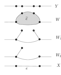
Figure 5. Example of a single-cell aggregation presented as an expansion followed by a sequence of collapses.

Here one can regard $W$ as $(Y\cup_{X-e}X)\cup\widetilde{e}$; the boundary of the cell $\widetilde{e}$ is $\partial\widetilde{e}=\bar{e}\cup_{\partial e}\bar{e}_{Y}$, where $e_{Y}=Y|_{e}$ is a copy $e$ subdivided in $Y$, which is glued to a non-subdivided copy of $e$ along the equator $\partial e=\partial e_{Y}$ in the sphere $\partial\widetilde{e}$.

Consider the standard cellular action $S_{W}$ for $W$. We have the standard induction data (142) for the collapses $W\searrow\cdots\searrow X$ which compose to $C^{\bullet}(W)\stackrel{{\scriptstyle(i_{W\rightarrow X},p_{W\rightarrow X},K_{W\rightarrow X})}}{{\rightsquigarrow}}C^{\bullet}(X)$ and also a standard induction data $C^{\bullet}(W)\stackrel{{\scriptstyle(i_{W\rightarrow Y},p_{W\rightarrow Y},K_{W\rightarrow Y})}}{{\rightsquigarrow}}C^{\bullet}(Y)$ for the collapse $W\searrow Y$. By Lemma 8.19, we have

(150) $$P_{*}^{W\rightarrow X}\left(e^{\frac{i}{\hbar}S_{W}}(\mu_{\mathsf{F}_{W}}^{\hbar})^{1/2}\right) =e^{\frac{i}{\hbar}S_{X}}(\mu_{\mathsf{F}_{X}}^{\hbar})^{1/2}+\Delta_{X}\left(-i\hbar\,r_{W\rightarrow X}\cdot e^{\frac{i}{\hbar}S_{X}}(\mu_{\mathsf{F}_{X}}^{\hbar})^{1/2}\right),$$

(151) $$P_{*}^{W\rightarrow Y}\left(e^{\frac{i}{\hbar}S_{W}}(\mu_{\mathsf{F}_{W}}^{\hbar})^{1/2}\right) =e^{\frac{i}{\hbar}S_{Y}}(\mu_{\mathsf{F}_{Y}}^{\hbar})^{1/2}+\Delta_{Y}\left(-i\hbar\,r_{W\rightarrow Y}\cdot e^{\frac{i}{\hbar}S_{Y}}(\mu_{\mathsf{F}_{Y}}^{\hbar})^{1/2}\right)$$

for some degree $-1$ functions $r_{W\rightarrow X}(\mathsf{A}_{X}|_{\bar{e}})$ and $r_{W\rightarrow Y}(\mathsf{A}_{Y}|_{\bar{e}_{Y}})$. Here for the BV pushforwards we use the gauge-fixing associated with the standard induction data above. For the pushforward $P_{*}^{Y\rightarrow X}$ corresponding to the aggregation $Y\rightarrow X$, we will use the induction data

(152) $$C^{\bullet}(Y)\stackrel{{\scriptstyle(p_{W\rightarrow Y}\circ i_{W\rightarrow X},p_{W\rightarrow X}\circ i_{W\rightarrow Y},p_{W\rightarrow Y}\circ K_{W\rightarrow X}\circ i_{W\rightarrow Y})}}{{\rightsquigarrow}}C^{\bullet}(X)$$

– this is the “geometric” gauge-fixing mentioned in the Proposition; it depends on choosing a particular presentation (149) of an aggregation as a simple-homotopy equivalence.

Composition of this data with $C^{\bullet}(W)\stackrel{{\scriptstyle}}{{\rightsquigarrow}}C^{\bullet}(Y)$ above yields the data $C^{\bullet}(W)\stackrel{{\scriptstyle}}{{\rightsquigarrow}}C^{\bullet}(X)$ above. Thus with these choices one has $P_{*}^{Y\rightarrow X}P_{*}^{W\rightarrow Y}=P_{*}^{W\rightarrow X}$ (a precise identity, not modulo canonical transformations); applying this to $e^{\frac{i}{\hbar}S_{W}}(\mu_{\mathsf{F}_{W}}^{\hbar})^{1/2}$ and using (150,151), we obtain

(153) $$P_{*}^{Y\rightarrow X}\left(e^{\frac{i}{\hbar}S_{Y}}(\mu_{\mathsf{F}_{Y}}^{\hbar})^{1/2}\right)=\\ =e^{\frac{i}{\hbar}S_{X}}(\mu_{\mathsf{F}_{X}}^{\hbar})^{1/2}+\Delta_{X}\left(-i\hbar\,r_{Y\rightarrow X}\cdot e^{\frac{i}{\hbar}S_{X}}(\mu_{\mathsf{F}_{X}}^{\hbar})^{1/2}\right)=:e^{\frac{i}{\hbar}S^{\prime}_{X}}(\mu_{\mathsf{F}_{X}}^{\hbar})^{1/2}$$

with $r_{Y\rightarrow X}(\mathsf{A}_{X}|_{\bar{e}}):=r_{W\rightarrow X}-e^{-\frac{i}{\hbar}S_{X}}P_{*}^{Y\rightarrow X}\left(r_{W\rightarrow Y}\cdot e^{\frac{i}{\hbar}S_{Y}}(\mu_{\mathsf{F}_{Y}}^{\hbar})^{1/2}\right)\in\mathrm{Fun}_{-1}(C^{\bullet}(\bar{e},\mathfrak{g})[1])$. We then define $R^{(1)}(\mathsf{A}_{X}|_{\bar{e}})$ as $R^{(1)}:=r_{Y\rightarrow X}\cdot\frac{\phi}{e^{\phi}-1}$ with $\phi(\mathsf{A}_{X}|_{\bar{e}}):=\frac{i}{\hbar}(S^{\prime}_{X}-S_{X})\in\mathrm{Fun}_{0}(C^{\bullet}(\bar{e},\mathfrak{g})[1])$. Then, by a calculation similar to the one in the proof of Lemma 8.19, (153) is equivalent to (147). This proves the Proposition in the case when $Y$ is a single-cell subdivision of $X$.

In the case of a general (non single-cell) aggregation (148), we notice that $S^{\prime}_{X}$, defined via $e^{\frac{i}{\hbar}S^{\prime}_{X}}(\mu_{\mathsf{F}_{X}}^{\hbar})^{1/2}:=P_{*}^{Y\rightarrow X}\left(e^{\frac{i}{\hbar}S_{Y}}(\mu_{\mathsf{F}_{Y}}^{\hbar})^{1/2}\right)$, with $P_{*}^{Y\rightarrow X}=P_{*}^{X_{1}\rightarrow X}\cdots P_{*}^{Y\rightarrow X_{m-1}}$, satisfies the assumptions of Lemma 8.7 and thus is connected to $S_{X}$ by a canonical transformation with generator satisfying the ansatz (115,116). From the single-cell aggregation case we infer that the generator has only the linear in $\hbar$ part (while the $\hbar$-independent part vanishes). Such a transformation with a $t$-dependent generator $-i\hbar\,R^{(1)}_{t}$, $t\in[0,1]$ is equivalent to a transformation with constant ($t$-independent) generator $-i\hbar\,R^{(1)}=-i\hbar\,\int_{0}^{1}dt\,R^{(1)}_{t}$. ∎

8.4. Remarks

In this section we comment on the BV cohomology defined by the theory. We also prove that the theory converges in an appropriate sense, in the limit of dense triangulation (here we restrict to the simplicial case), to the standard continuum $BF$ theory on a manifold.

8.4.1. BV cohomology

Definition 8.23.

Let $\mathsf{F},\omega$ be an odd-symplectic space and $S\in\mathrm{Fun}_{0}(\mathsf{F})[[-i\hbar]]$ a solution of the quantum master equation on $\mathsf{F}$. We define the perturbative BV cohomology at $S$ as the cohomology of the differential $\delta_{S}=\{S,\bullet\}-i\hbar\Delta=e^{-\frac{i}{\hbar}S}\Delta e^{\frac{i}{\hbar}S}$ on $\mathrm{Fun}(\mathsf{F})[[-i\hbar]]$.

In particular, cohomology of $\delta_{S}$ in degree zero controls infinitesimal deformations of $S$ as a solution of QME modulo canonical transformations (or, in other words, gives observables $O\in\mathrm{Fun}_{0}(\mathsf{F})[[-i\hbar]]$ such that $\Delta(O\,e^{\frac{i}{\hbar}S})=0$ considered modulo infinitesimal equivalence $O\,e^{\frac{i}{\hbar}S}\sim O\,e^{\frac{i}{\hbar}S}+\epsilon\,\Delta(-i\hbar\,R\,e^{\frac{i}{\hbar}S})$).

Assume that we are in the setting of Section 8.2.1, with $\mathsf{F}=V[1]\oplus V^{*}[-2]$ for $V=V^{\bullet}$ a graded vector space and $S$ satisfying the $BF_{\infty}$ ansatz (131). We note the following.

1. Cohomology of $\Delta$ on $\mathrm{Fun}(\mathsf{F})$ is a line spanned by the element $\nu\in\bigotimes_{k}\mathrm{Det}(V^{2k})^{*}\otimes\bigotimes_{k}\mathrm{Det}\,V^{2k+1}=\mathrm{Det}(\mathsf{F}^{\mathrm{odd}})^{*}$ given by the product of all components of $\mathsf{A}$ ,$\mathsf{B}$ of odd internal degree, $H_{\Delta}(\mathrm{Fun}(\mathsf{F}))=\nu\cdot\mathbb{R}$, with $\nu$ having internal degree $|\nu|=\sum_{k}(1-2k)\dim V^{2k}+\sum_{k}(-2+(2k+1))\dim V^{2k+1}$. This cohomology was considered in [15].

2. We have

   (154) $$H^{k}_{\{S^{(0)},\bullet\}}(\mathrm{Fun}(\mathsf{F}))=H^{k}_{CE}(V,\mathrm{Sym}\,V[2])$$

   where on the r.h.s. we have the Chevalley-Eilenberg cohomology of the $L_{\infty}$ algebra $V,\{l_{n}\}$ (with $l_{n}$ the $L_{\infty}$ operations corresponding to the $O(\hbar^{0})$ term in $S$ via (132)) with coefficients in the sum of symmetric powers of the adjoint module. We denote the cohomology (154) by $\mathfrak{H}$ – one can view it as the “classical” ($\hbar$-independent) counterpart of perturbative BV cohomology.

3. The operator $\{S^{(1)},\bullet\}+\Delta$ can be viewed as a perturbation of the differential $\{S^{(0)},\bullet\}$ on $\mathrm{Fun}(\mathsf{F})$ and thus induces, by homological perturbation theory (HPT) a differential $\mathfrak{D}$ on $\mathfrak{H}$. We then have

   (155) $$H^{\bullet}_{\delta_{S}}(\mathrm{Fun}(\mathsf{F})[[-i\hbar]])=H^{\bullet}_{-i\hbar\mathfrak{D}}(\mathfrak{H}[[-i\hbar]])=\left(\mathfrak{H}^{\bullet}\cap\ker\mathfrak{D}\right)\oplus(-i\hbar)\cdot H^{\bullet}_{\mathfrak{D}}(\mathfrak{H})[[-i\hbar]]$$

   This means that the perturbative BV cohomology in the order $O(\hbar^{0})$ is given by $\mathfrak{D}$-closed elements of classical BV cohomology (154), whereas in positive orders in $\hbar$ it is given by copies of cohomology of $\mathfrak{D}$, one copy per order.

4. Consider the “abelian $BF$” action $S^{\mathrm{ab}}:=\left\langle\mathsf{B},d\mathsf{A}\right\rangle$ on $\mathsf{F}$, for $d=l_{1}$ the differential on $V$, – it is the quadratic $\hbar$-independent term of the full $BF_{\infty}$ action $S$. We have $H^{\bullet}_{\{S^{\mathrm{ab}},\bullet\}}(\mathrm{Fun}(\mathsf{F}))=\mathrm{Fun}(\mathsf{F}_{\mathrm{res}})$ with $\mathsf{F}_{\mathrm{res}}=H^{\bullet}(V)[1]\oplus(H^{\bullet}(V))^{*}[-2]$ and the perturbation of the differential $\{S^{\mathrm{ab}},\bullet\}\mapsto\{S^{\mathrm{ab}},\bullet\}+\Delta$ produces, as the induced differential, the standard BV Laplacian $\Delta_{\mathrm{res}}$ on $\mathrm{Fun}(\mathsf{F}_{\mathrm{res}})$. In particular, we have

   (156) $$H^{\bullet}_{\{S^{\mathrm{ab}},\bullet\}-i\hbar\Delta}=H^{\bullet}_{-i\hbar\Delta_{\mathrm{res}}}(\mathrm{Fun}(\mathsf{F}_{\mathrm{res}})[[-i\hbar]])=\left(\mathrm{Fun}(\mathsf{F}_{\mathrm{res}})\cap\ker\Delta_{\mathrm{res}}\right)\oplus(-i\hbar)\nu_{\mathrm{res}}\cdot\mathbb{R}[[-i\hbar]]$$

   with $\nu_{\mathrm{res}}$ as in (i), with $V$ replaced by $H^{\bullet}(V)$.

5. Assume that $V^{\prime},d^{\prime}$ is a retract of the complex $V,d$ and assume that $S^{\prime}$ is the effective action on $\mathsf{F}^{\prime}=V^{\prime}[1]\oplus(V^{\prime})^{*}[-2]$ induced from $S$ via BV pushforward. Note that $S^{\prime}$ automatically satisfies $BF_{\infty}$ ansatz. Then, treating $\delta_{S}$ via HPT as a perturbation of the differential $\{S^{\mathrm{ab}},\bullet\}-i\hbar\Delta$ on $\mathrm{Fun}(\mathsf{F})[[-i\hbar]]$, one can prove that the induced differential on $\mathrm{Fun}(\mathsf{F}^{\prime})[[-i\hbar]]$ is precisely $\delta_{S^{\prime}}$, with $S^{\prime}$ given by Feynman diagrams for the BV pushforward (a version of this observation was made in [16]; this statement is not specific to $BF_{\infty}$ ansatz).Therefore, we have

   (157) $$H^{\bullet}_{\delta_{S}}(\mathrm{Fun}(\mathsf{F})[[-i\hbar]])=H^{\bullet}_{\delta_{S^{\prime}}}(\mathrm{Fun}(\mathsf{F}^{\prime})[[-i\hbar]])$$

6. Let $S_{\mathrm{res}}=S_{\mathrm{res}}^{(0)}-i\hbar\,S_{\mathrm{res}}^{(1)}\in\mathrm{Fun}(\mathsf{F}_{\mathrm{res}})[[-i\hbar]]$ be the effective action induced on $\mathsf{F}_{\mathrm{res}}$ from $S$. Denote $w:=\left.S_{\mathrm{res}}\right|_{\hbar=i}=S_{\mathrm{res}}^{(0)}+S_{\mathrm{res}}^{(1)}\in\mathrm{Fun}(\mathsf{F}_{\mathrm{res}})$. Using (v) and (iv), we see that the cohomology

   (158) $$H^{\bullet}_{\mathfrak{D}}(\mathfrak{H})=H^{\bullet}_{\{w,\bullet\}+\Delta_{\mathrm{res}}}(\mathrm{Fun}(\mathsf{F}_{\mathrm{res}}))=e^{-w}\nu_{\mathrm{res}}\cdot\mathbb{R}$$

   has rank $1$ and is concentrated in degree $|\nu_{\mathrm{res}}|=\sum_{k}(1-2k)(\dim H^{2k}(V)-\dim H^{2k+1}(V))$.

7. Putting together (iii) and (vi), we obtain that

   (159) $$H^{\bullet}_{\delta_{S}}(\mathrm{Fun}(\mathsf{F})[[-i\hbar]])=(\mathfrak{H}^{\bullet}\cap\ker\mathfrak{D})\oplus(-i\hbar)e^{-w}\nu_{\mathrm{res}}\cdot\mathbb{R}[[-i\hbar]]$$

Summarizing the observations above and applying to the case of cellular action of Theorem 8.6, and using Proposition 8.20, we have the following.

Proposition 8.24.

For $X$ a regular CW complex, perturbative BV cohomology associated to the cellular action (116) has the form

(160) $$H^{\bullet}_{\delta_{S_{X}}}(\mathrm{Fun}(\mathsf{F}_{X})[[-i\hbar]])=(\mathfrak{H}^{\bullet}_{X}\cap\ker\mathfrak{D}_{X})\oplus(-i\hbar)\cdot\mathbb{R}[-\mathfrak{p}][[-i\hbar]]$$

where

• $\mathfrak{H}^{\bullet}=H^{\bullet}_{CE}(C(X,\mathfrak{g}),\mathrm{Sym}\,C(X,\mathfrak{g})[2])\cong H^{\bullet}_{CE}(H(X,\mathfrak{g}),\mathrm{Sym}\,H(X,\mathfrak{g})[2])$ – Chevalley-Eilenberg cohomology of cellular cochains and cellular cohomology, understood as $L_{\infty}$ algebras, with coefficients in the sum of symmetric powers of the adjoint module.

• $\mathfrak{D}_{X}$ is the differential on $\mathfrak{H}^{\bullet}$ induced by homological perturbation theory from the perturbation $\{S^{(0)},\bullet\}\mapsto\{S^{(0)},\bullet\}+\{S^{(1)}_{X},\bullet\}+\Delta_{X}$ of the differential on $\mathrm{Fun}(\mathsf{F}_{X})$. Equivalently, $\mathfrak{D}_{X}$ is induced from the perturbation $\{S^{(0)}_{\mathrm{res}},\bullet\}\mapsto\{S^{(0)}_{\mathrm{res}},\bullet\}+\{S^{(1)}_{\mathrm{res}},\bullet\}+\Delta_{\mathrm{res}}$ of the differential on $\mathrm{Fun}(\mathsf{F}_{\mathrm{res}})$.

• Perturbative BV cohomology in higher orders in $\hbar$ has rank $1$ and is concentrated in degree

  $$\mathfrak{p}=\sum_{k}(1-2k)\left(\dim H^{2k}(X,\mathfrak{g})-\dim H^{2k+1}(X,\mathfrak{g})\right)$$

• The generator $1\in\mathbb{R}$ of perturbative BV cohomology in positive degree in $\hbar$ is represented in $\mathrm{Fun}(\mathsf{F}_{X})$ by the element $p^{*}(e^{-w}\nu_{\mathrm{res}})$ where $p:\mathsf{F}_{X}\rightarrow\mathsf{F}_{\mathrm{res}}$ is the projection to residual fields used as a part of gauge-fixing in (136), $\nu_{\mathrm{res}}\in\bigotimes_{k}\mathrm{Det}(H^{2k}(X,\mathfrak{g}))^{*}\otimes\bigotimes_{k}\mathrm{Det}(H_{2k+1}(X,\mathfrak{g}^{*}))^{*}=\mathrm{Det}(\mathsf{F}_{\mathrm{res}}^{\mathrm{odd}})^{*}$ is the product of all components of fields $\mathsf{A}_{\mathrm{res}},\mathsf{B}_{\mathrm{res}}$ of odd internal degree; $w=S^{(0)}_{\mathrm{res}}+S^{(1)}_{\mathrm{res}}$ is the effective action on residual fields evaluated at $\hbar=i$.

If the complexes $X$ and $Y$ are simple-homotopy equivalent, the respective BV cohomology is canonically isomorphic,

$$H^{\bullet}_{\delta_{S_{X}}}(\mathrm{Fun}(\mathsf{F}_{X})[[-i\hbar]])\cong H^{\bullet}_{\delta_{S_{Y}}}(\mathrm{Fun}(\mathsf{F}_{Y})[[-i\hbar]])$$

Example 8.25.

For $X$ contractible, perturbative BV cohomology is the same as for $X$ a point, and thus we have $H^{\bullet}_{\delta_{S_{X}}}=(H^{\bullet}_{CE}(\mathfrak{g},\mathrm{Sym}\,\mathfrak{g}[2])\cap\ker\mathfrak{D})\oplus(-i\hbar)\mathbb{R}[-\dim\mathfrak{g}][[-i\hbar]]$. One can understand $H^{\bullet}_{CE}(\mathfrak{g},\mathrm{Sym}\,\mathfrak{g}[2])\cap\ker\mathfrak{D}$ as the subspace of unimodular classes in Lie algebra cohomology. For example, in degree zero we have $H^{0}_{\delta_{S_{X}}}=\bigoplus_{k}H^{2k}_{CE}(\mathfrak{g},\mathrm{Sym}\,^{k}\mathfrak{g})\cap\ker\mathfrak{D}$. Contribution of $k=1$ here is the space of unimodular deformations of the Lie bracket on $\mathfrak{g}$ modulo inner automorphisms (note that for $\mathfrak{g}$ semi-simple, it vanishes since $H^{2}_{CE}(\mathfrak{g},\mathfrak{g})$ vanishes as a whole).

Example 8.26.

For $X$ arbitrary and $\mathfrak{g}$ an abelian Lie algebra, perturbative BV cohomology is given by (156). If we identify $\mathrm{Fun}(\mathsf{F}_{\mathrm{res}})$ with polyvector fields on $H^{\bullet}(X,\mathfrak{g})[1]$, then $\mathrm{Fun}(\mathsf{F}_{\mathrm{res}})\cap\ker\Delta_{\mathrm{res}}$ is the subspace of divergence-free polyvector fields.

Returning to the setup of Section 8.2.1, we can introduce a subspace

$$\Xi:=\\ :=\{\left\langle\mathsf{B},\alpha(\mathsf{A})\right\rangle-i\hbar\,\beta(\mathsf{A})\;\Big{|}\;\alpha(\mathsf{A})\in\widehat{\mathrm{Sym}\,^{\geq 2}}(V[1])^{*}\otimes V^{*},\beta(\mathsf{A})\in\widehat{\mathrm{Sym}\,^{\geq 1}}(V[1])^{*}\}\\ =\Xi^{(0)}\oplus(-i\hbar)\cdot\Xi^{(1)}\quad\subset\mathrm{Fun}(\mathsf{F})[[-i\hbar]]$$

– elements satisfying the $BF_{\infty}$ ansatz (131) with terms bi-linear in $\mathsf{A}$ and $\mathsf{B}$ prohibited. Note that $\Xi$ is a subcomplex w.r.t. $\delta_{S}$. Repeating the argument above, we obtain that the cohomology of $\delta_{S}$ on $\Xi$ is

$$H^{\bullet}_{\delta_{S}}(\Xi)=H^{\bullet}_{\{S^{(0)},\bullet\}}(\Xi^{(0)})\cap\ker\mathfrak{D}$$

with $\mathfrak{D}$ as above; note that this cohomology does not have $O(\hbar^{\geq 1})$ terms.

Remark 8.27.

Note that $-i\hbar\cdot 1$ is a $\delta_{S}$-exact element in $\mathrm{Fun}(\mathsf{F})[[-i\hbar]]$. By inspecting the HPT argument above, one can construct an explicit primitive $\phi(\mathsf{A},\mathsf{B})$ with $\delta_{S}(\phi)=-i\hbar\cdot 1$; this element necessarily contains a component bi-linear in $\mathsf{A}$ and $\mathsf{B}$. Therefore, for any $c\in\mathbb{R}$ one can connect $S$ and $S-i\hbar\cdot c$ (or, equivalently, half-densities $e^{\frac{i}{\hbar}S}(\mu_{\mathsf{F}}^{\hbar})^{1/2}$ and $e^{c}\cdot e^{\frac{i}{\hbar}S}(\mu_{\mathsf{F}}^{\hbar})^{1/2}$) by a canonical transformation. But if the generator of the canonical transformation is prohibited to have a term bi-linear in $\mathsf{A}$, $\mathsf{B}$, then such transformation is prohibited. Thus our rigid normalization of half-densities $e^{\frac{i}{\hbar}S_{X}}(\mu_{\mathsf{F}_{X}}^{\hbar})^{1/2}$ and $Z$ (as defined by (136)) is meaningful, since the restriction above for canonical transformations holds in all cases of relevance for us: in Lemmata 8.7, 8.19, in (137) and Propositions 8.20 and 8.22.

8.4.2. Continuum limit

Simplicial $BF$ action (107) approximates the standard action of non-abelian $BF$ theory defined on differential forms on a manifold, in the limit of “dense” triangulation, in the following sense.

Let $M$ be a smooth compact oriented $n$-dimensional manifold endowed with a Riemannian metric $g$. Let $\{X_{N}\}$ for $N=1,2,\ldots$ be a sequence of triangulations of $M$ with the property that metric diameters of simplices of $X_{N}$ are bounded from above by $c/N$ for $c$ a constant. Fix $(A,B)\in\Omega^{\bullet}(M,\mathfrak{g})[1]\oplus\Omega^{\bullet}(M,\mathfrak{g})[n-2]$ a pair of smooth non-homogeneous differential forms. We project this pair to an element of the cellular space of fields, $(\mathsf{A}_{N},\mathsf{B}_{N})\in\mathsf{F}_{X_{N}}$, with $\mathsf{A}_{N}:=\sum_{e\subset X_{N}}e^{*}\cdot\left(\int_{e}A\right)$, $\mathsf{B}_{N}:=\sum_{e\subset X_{N}}\left(\int_{M}B\wedge\chi_{e}\right)\cdot e$ where $\chi_{e}$ is a piecewise-linear form on $M$ of degree $\dim e$ – the Whitney form associated to $e$.

Lemma 8.28.

We have the following asymptotics for the value of the $\hbar$-independent part of the simplicial action $S^{(0)}_{X_{N}}$ on $(\mathsf{A}_{N},\mathsf{B}_{N})$:

(161) $$S_{X_{N}}^{(0)}(\mathsf{A}_{N},\mathsf{B}_{N})\underset{N\rightarrow\infty}{\sim}\int_{M}\left\langle B\stackrel{{\scriptstyle\wedge}}{{,}}dA+\frac{1}{2}[A\stackrel{{\scriptstyle\wedge}}{{,}}A]\right\rangle_{\mathfrak{g}}+O\left(\frac{1}{N}\right)$$

The first term on the r.h.s. is the standard action of non-abelian $BF$ theory in BV formalism, see e.g. [7, 27, 4].

Proof.

Let $i_{N}:C^{\bullet}(X_{N})\rightarrow\Omega^{\bullet}(M)$ be the inclusion of cellular cochains of the triangulation into piecewise-polynomial forms given by Whitney forms, and let $p_{N}:\Omega^{\bullet}(M)\rightarrow C^{\bullet}(X_{N})$ be the Poincaré projection, as in Section 8.1. Then, for $\alpha$ any smooth form on $M$, we have

(162) $$\alpha-i_{N}\circ p_{N}(\alpha)=O\left(\frac{1}{N}\right)$$

In particular, $A-i_{N}(\mathsf{A}_{N})=O\left(\frac{1}{N}\right)$ and $[A\stackrel{{\scriptstyle\wedge}}{{,}}A]-i_{N}([\mathsf{A}_{N},\stackrel{{\scriptstyle*}}{{,}}\mathsf{A}_{N}])=O\left(\frac{1}{N}\right)$.

Note that components of the cellular field $(\mathsf{A}_{N},\mathsf{B}_{N})$ on simplices of $X_{N}$ behave in the asymptotics $N\rightarrow\infty$ as $\mathsf{A}_{e}=O(N^{-\dim e})$, $\mathsf{B}_{e}=O(N^{-n+\dim e})$. The number of simplices $e$ of $X^{N}$ of any fixed dimension behaves as $O(N^{n})$. Thus, we can estimate the term

$$S^{(0),k}:=\sum_{e\subset X_{N}}\sum_{\Gamma_{0}}\sum_{e_{1},\ldots,e_{k}\subset\bar{e}}\frac{1}{|\mathrm{Aut}(\Gamma_{0})|}C^{e}_{\Gamma_{0},e_{1},\ldots,e_{k}}\left\langle\mathsf{B}_{e},\mathrm{Jacobi}_{\Gamma_{0}}(\mathsf{A}_{e_{1}},\ldots,\mathsf{A}_{e_{k}})\right\rangle$$

in the cellular action $S_{X_{N}}$ as $O(N^{n}\cdot N^{-n+\dim e-\dim e_{1}-\cdots-\dim e_{k}})=O(N^{2-k})$ (where we use the relation $\dim e-\dim e_{1}-\cdots-\dim e_{k}=2-k$ between dimensions of the $k$-tuple of faces of $e$, which arises from the fact that the associated monomial in components of fields, $\left\langle\mathsf{B}_{e},\mathrm{Jacobi}_{\Gamma_{0}}(\mathsf{A}_{e_{1}},\ldots,\mathsf{A}_{e_{k}})\right\rangle$, should have internal degree zero). In particular, we have

(163) $$\sum_{k\geq 3}S^{(0),k}(\mathsf{A}_{N},\mathsf{B}_{N})=O\left(\frac{1}{N}\right)$$

On the other hand, by (108) we have $S^{(0)}_{X_{N}}=\left\langle\mathsf{B}_{N},d\mathsf{A}_{N}\right\rangle+\frac{1}{2}\left\langle\mathsf{B}_{N},[\mathsf{A}_{N}\stackrel{{\scriptstyle*}}{{,}}\mathsf{A}_{N}]\right\rangle+\sum_{k\geq 3}S^{(0),k}(\mathsf{A}_{N},\mathsf{B}_{N})$ and

$$\left(\left\langle\mathsf{B}_{N},d\mathsf{A}_{N}\right\rangle+\frac{1}{2}\left\langle\mathsf{B}_{N},[\mathsf{A}_{N}\stackrel{{\scriptstyle*}}{{,}}\mathsf{A}_{N}]\right\rangle\right)-\int_{M}\left\langle B\stackrel{{\scriptstyle\wedge}}{{,}}dA+\frac{1}{2}[A\stackrel{{\scriptstyle\wedge}}{{,}}A]\right\rangle_{\mathfrak{g}}\\ =\int_{M}\left\langle B\stackrel{{\scriptstyle\wedge}}{{,}}(i_{N}\circ p_{N}-\mathrm{id})\left(dA+\frac{1}{2}[A\stackrel{{\scriptstyle\wedge}}{{,}}A]\right)\right\rangle_{\mathfrak{g}}\quad=O\left(\frac{1}{N}\right)$$

where we used (162). Together with the estimate (163), this finishes the proof of the Lemma.

∎

Remark 8.29.

For the linear in $\hbar$ part of the simplicial action $S^{(1)}_{X_{N}}$, similar estimates yield $S^{(1),k}(\mathsf{A}_{N})=O(N^{n-k})$ (for the part of homogeneous degree $k$ in $\mathsf{A}_{N}$) and $S^{(1)}_{X_{N}}(\mathsf{A}_{N})=O(N^{n-2})$ for the whole.

Remark 8.30.

In Lemma 8.28, one can allow $X_{N}$ to be a sequence of prismatic cellular decompositions of $M$ instead of triangulations (with the same bound $c/N$ on the diameters of prisms), according to Remark 8.5.

9. Non-abelian cellular $BF$ theory, II: case of a cobordism

In this section we address the construction of non-abelian cellular $BF$ theory in the formalism of Section 6.

Fix $G$ a Lie group with bi-invariant Haar measure $\mu_{G}$. The Lie algebra $\mathfrak{g}=\mathrm{Lie}(G)$ is automatically unimodular and carries the induced density $\mu_{\mathfrak{g}}$.

Let $M$ be a compact oriented piecewise-linear $n$-manifold with boundary $\partial M=\overline{M_{\mathrm{in}}}\sqcup M_{\mathrm{out}}$. Let $(P,\nabla_{P})$ be a flat $G$-bundle over $M$ and $(E,\nabla_{E})$ the vector bundle associated to $P$ via adjoint representation, $E=\mathrm{Ad}(P)=P\times_{G}\mathfrak{g}$; by construction it carries a horizontal fiberwise density $\mu_{E}$ induced from $\mu_{G}$. Let $X$ be a cellular decomposition of $M$; we assume that $X$ is a regular CW complex of product type near the boundary $X_{\mathrm{out}}$ (see Definition 2.4). We call such $X$ an admissible cellular decomposition of $M$.

We import directly from Section 6, without changes, the construction of:

• The space of fields $\mathcal{F}=C^{\bullet}(X,E)[1]\oplus C^{\bullet}(X^{\vee},E^{*})[n-2]$. (By a slight abuse of notation, we omit subscripts in $E_{X}$ and $E^{*}_{X^{\vee}}$.)

• The superfields

  $$A=\sum_{e\subset X}e^{*}\cdot A_{e}:\;\mathcal{F}\rightarrow C^{\bullet}(X,E),\qquad B=\sum_{e^{\vee}\subset X^{\vee}}B_{e^{\vee}}\cdot(e^{\vee})^{*}:\;\mathcal{F}\rightarrow C^{\bullet}(X^{\vee},E^{*})$$

  Note that $B$ is again a cochain, unlike in the formalism of Section 8.1.

• The presymplectic 2-form $\omega=\left\langle\delta B,\delta A\right\rangle$.

• The boundary fields $\mathcal{F}_{\partial}=C^{\bullet}(X_{\partial},E)[1]\oplus C^{\bullet}(X_{\partial}^{\vee},E^{*})[n-2]$.

• The symplectic form $\omega_{\partial}$ and its primitive 1-form $\alpha_{\partial}$.

• The projection $\pi:\mathcal{F}\twoheadrightarrow\mathcal{F}_{\partial}$. Later we will need to deform it, see (168) below.

We define the action $S(A,B;\hbar)\in\mathrm{Fun}(\mathcal{F})_{0}[[\hbar]]$ as follows:

(164) $$S(A,B;\hbar):=\sum_{e\subset X-X_{\mathrm{out}}}\bar{S}_{e}(A|_{\bar{e}},B_{\varkappa(e)};\hbar)+\left\langle B,A\right\rangle_{\mathrm{in}}\\ =\sum_{e\subset X-X_{\mathrm{out}}}\sum_{k\geq 1}\frac{1}{k!}\left\langle B_{\varkappa(e)},l_{k}^{e}\left(A|_{\bar{e}},\cdots,A|_{\bar{e}}\right)\right\rangle-i\hbar\sum_{e\subset X-X_{\mathrm{out}}}\sum_{k\geq 2}\frac{1}{k!}q_{k}^{e}\left(A|_{\bar{e}},\cdots,A|_{\bar{e}}\right)+\left\langle B,A\right\rangle_{\mathrm{in}}$$

with $\bar{S}_{e}$ the building blocks (115) of Theorem 8.6 and $l_{k}^{e},q_{k}^{e}$ the corresponding components of the operations of the unimodular $L_{\infty}$ algebra coming from (135). In (164) we use the parallel transport $E(e>e^{\prime})$ to trivialize the coefficient local system over the cell $e$ (see (7)) and we set

(165) $$A|_{\bar{e}}:=\sum_{e^{\prime}\subset e}(e^{\prime})^{*}\cdot\mathrm{Ad}_{E(e>e^{\prime})}A_{e^{\prime}}:\quad\mathcal{F}\rightarrow C^{\bullet}(\bar{e})\otimes\mathfrak{g}$$

We also use a shorthand notation $\left\langle B,A\right\rangle_{\mathrm{in}}:=\left\langle(\iota^{\vee})^{*}B,\iota^{*}A\right\rangle_{\mathrm{in}}=\sum_{e\subset X_{\mathrm{in}}}\left\langle B_{\varkappa_{\mathrm{in}}(e)},A_{e}\right\rangle$ for the boundary term of the action, as in (64). As in Section 8, the action has the structure $S=S^{(0)}-i\hbar\,S^{(1)}$.

We also define $S_{\partial}=S_{\mathrm{out}}-S_{\mathrm{in}}\in\mathrm{Fun}_{1}(\mathcal{F}_{\partial})$ by

(166) $$\!\!\!\!\!\!\!\!S_{\partial}(A_{\partial},B_{\partial}):=\sum_{e\subset X_{\mathrm{out}}}\sum_{k\geq 1}\frac{1}{k!}\left\langle B_{\varkappa_{\mathrm{out}}(e)},l_{k}^{e}\left(A|_{\bar{e}},\cdots,A|_{\bar{e}}\right)\right\rangle-\sum_{e\subset X_{\mathrm{in}}}\sum_{k\geq 1}\frac{1}{k!}\left\langle B_{\varkappa_{\mathrm{in}}(e)},l_{k}^{e}\left(A|_{\bar{e}},\cdots,A|_{\bar{e}}\right)\right\rangle$$

Further, we introduce the vector field $Q^{(0)}\in\mathfrak{X}(\mathcal{F})_{1}$,

(167) $$Q^{(0)}=\sum_{e\subset X}\sum_{k\geq 1}(-1)^{\dim e}\frac{1}{k!}\left\langle l_{k}^{e}(A|_{\bar{e}},\cdots,A|_{\bar{e}}),\frac{\partial}{\partial A_{e}}\right\rangle-\\ -\sum_{e\subset X-X_{\mathrm{out}}}\sum_{k\geq 0}\frac{1}{k!}\left\langle B_{\varkappa(e)},l_{k+1}^{e}\left(A|_{\bar{e}},\cdots,A|_{\bar{e}},\sum_{e^{\prime}\subset\bar{e}-X_{\mathrm{out}}}(e^{\prime})^{*}\cdot\mathrm{Ad}_{E(e>e^{\prime})}\frac{\partial}{\partial B_{\varkappa(e^{\prime})}}\right)\right\rangle\\ +\sum_{e\subset X_{\mathrm{in}}}\sum_{k\geq 0}\frac{1}{k!}\left\langle B_{\varkappa_{\mathrm{in}}(e)},l_{k+1}^{e}\left(A|_{\bar{e}},\cdots,A|_{\bar{e}},\sum_{e^{\prime}\subset\bar{e}}(e^{\prime})^{*}\cdot\mathrm{Ad}_{E(e>e^{\prime})}\frac{\partial}{\partial B_{\varkappa_{\mathrm{in}}(e^{\prime})}}\right)\right\rangle\\ -\sum_{e\subset X_{\mathrm{in}}}\left\langle B_{\varkappa_{\mathrm{in}}(e)},\frac{\partial}{\partial B_{\varkappa(e)}}\right\rangle$$

Introduce the algebra homomorphism $\Pi^{*}:\;\mathrm{Fun}(\mathcal{F}_{\partial})\rightarrow\mathrm{Fun}(\mathcal{F})$ deforming the pullback by the standard projection $\pi^{*}$, defined on the generators as follows:

(168) $$\Pi^{*}:\left\{\begin{array}[]{l}A_{\mathrm{in}}\mapsto A_{\mathrm{in}}\\ B_{\mathrm{in}}\mapsto B_{\mathrm{in}}\\ A_{\mathrm{out}}\mapsto A_{\mathrm{out}}\\ \left\langle B_{\mathrm{out}},a\right\rangle_{\mathrm{out}}\mapsto\sum_{e\supset e^{\prime}}\sum_{k\geq 0}\frac{1}{k!}\left\langle B_{\varkappa(e)},l_{k}^{e}(A|_{\bar{e}},\cdots,A|_{\bar{e}},(e^{\prime})^{*}\cdot\mathrm{Ad}_{E(e>e^{\prime})}a_{e^{\prime}})\right\rangle\end{array}\right.$$

where $a=\sum_{e\subset X_{\mathrm{out}}}e^{*}\cdot a_{e}\in C^{\bullet}(X_{\mathrm{out}})$ is a test cochain; the sum is over pairs of cells $e\supset e^{\prime}$ such that $e^{\prime}\subset X_{\mathrm{out}}$ while $e\subset X-X_{\mathrm{out}}$.

The following is proven by a straightforward (but lengthy) computation, using the $\bmod\,\hbar$ part of the result of Theorem 8.1.

Proposition 9.1.

The data $(\mathcal{F},\omega,Q^{(0)},S^{(0)},\Pi^{*})$, $(\mathcal{F}_{\partial},\alpha_{\partial},S_{\partial})$ define a classical BV-BFV theory [4], i.e. the following relations hold:

1. $(Q^{(0)})^{2}=0$.

2. $\iota_{Q^{(0)}}\omega=\delta S^{(0)}+\Pi^{*}\alpha_{\partial}$.

3. $Q^{(0)}\Pi^{*}=\Pi^{*}Q_{\partial}$ where $Q_{\partial}\in\mathfrak{X}(\mathcal{F}_{\partial})_{1}$ is the Hamiltonian vector field generated by $S_{\partial}$, i.e. is defined by $\iota_{Q_{\partial}}\omega_{\partial}=\delta S_{\partial}$.

The space of states $\mathcal{H}_{\partial}=\mathrm{Fun}_{\mathbb{C}}(\mathcal{B}_{\partial})\ni\psi(B_{\mathrm{in}},A_{\mathrm{out}})$ is defined as in Section 7, with the base of polarization $\mathcal{B}_{\partial}$ the same as in (69).It splits as $\mathcal{H}_{\partial}=\mathcal{H}_{\mathrm{in}}^{(B)}\widehat{\otimes}\mathcal{H}_{\mathrm{out}}^{(A)}$, as in (72).

We define the degree $1$ operator $\widehat{S}_{\partial}=\widehat{S}_{\mathrm{out}}+\widehat{S}_{\mathrm{in}}$ on $\mathcal{H}_{\partial}$ as the quantization of $S_{\partial}$, obtained by replacing $B_{\varkappa_{\mathrm{out}}(e)}\mapsto-i\hbar(-1)^{\dim e}\frac{\partial}{\partial A_{e}}$ for $e\subset X_{\mathrm{out}}$ and $A_{e}\mapsto-i\hbar\frac{\partial}{\partial B_{\varkappa_{\mathrm{in}}(e)}}$ for $e\subset X_{\mathrm{in}}$ in (166) and putting all derivatives in $A$ or $B$ to the right.

Explicitly, for $\widehat{S}_{\mathrm{out}},\widehat{S}_{\mathrm{in}}$ we have

(169) $$\widehat{S}_{\mathrm{out}} = \sum_{e\subset X_{\mathrm{out}}}\sum_{k\geq 1}\frac{1}{k!}\left\langle l_{k}^{e}\left(A|_{\bar{e}},\cdots,A|_{\bar{e}}\right),-i\hbar\,(-1)^{\dim e}\frac{\partial}{\partial A_{e}}\right\rangle$$

(170) $$\widehat{S}_{\mathrm{in}} = \sum_{e\subset X_{\mathrm{in}}}\sum_{k\geq 1}\frac{1}{k!}\left\langle B_{\varkappa_{\mathrm{in}}(e)},l_{k}^{e}\left(\widehat{A}|_{\bar{e}},\cdots,\widehat{A}|_{\bar{e}}\right)\right\rangle$$

where $\widehat{A}|_{\bar{e}}:=-i\hbar\sum_{e^{\prime}\subset\bar{e}}(e^{\prime})^{*}\cdot\mathrm{Ad}_{E(e>e^{\prime})}\frac{\partial}{\partial B_{\varkappa_{\mathrm{in}}(e^{\prime})}}$.

It is convenient to introduce, alongside $\widehat{S}_{\mathrm{out}}$, its version acting on out-states from the right,

(171) $$\overleftarrow{\widehat{S}}_{\mathrm{out}}=\sum_{e\subset X_{\mathrm{out}}}\sum_{k\geq 1}\frac{1}{k!}\left\langle-i\hbar\,\frac{\overleftarrow{\partial}}{\partial A_{e}},l_{k}^{e}\left(A|_{\bar{e}},\cdots,A|_{\bar{e}}\right)\right\rangle$$

It satisfies $\widehat{S}_{\mathrm{out}}\psi=(-1)^{|\psi|+1}\psi\overleftarrow{\widehat{S}}_{\mathrm{out}}$ for any $\psi=\psi(A_{\mathrm{out}})\in\mathcal{H}_{\mathrm{out}}^{(A)}$.

Remark 9.2.

For $Y$ a cellular decomposition of a closed $(n-1)$-manifold, the operators $\overleftarrow{\widehat{S}}_{Y}^{(A)}$ and $\widehat{S}_{Y}^{(B)}$ defined by formulae (171,170) on $Y$, are mutually adjoint w.r.t. the pairing (73):

$$(\phi\circ\overleftarrow{\widehat{S}}^{(A)}_{Y},\psi)=(\phi,\widehat{S}^{(B)}_{Y}\circ\psi)$$

for $\phi(A_{Y})\in\mathcal{H}_{Y}^{(A)}$ and $\psi(B_{Y})\in\mathcal{H}_{Y}^{(B)}$.

Proposition 9.3.

1. The operator $\widehat{S}_{\partial}$ defined as above squares to zero.

2. The action (164) on a cobordism $M$ endowed with an admissible cellular decomposition $X$ satisfies the modified quantum master equation:

   (172) $$\left(\frac{i}{\hbar}\widehat{S}_{\partial}-i\hbar\Delta_{\mathrm{bulk}}\right)\,e^{\frac{i}{\hbar}S}=0$$

Proof.

Part (a) is an immediate consequence of the classical $L_{\infty}$ relations (129) for the boundary complex $X_{\partial}$, which in turn follow from Theorem 8.1 applied to $X_{\partial}$.

Let us prove part (b). First, observe from (164) that $S$ depends on $B_{\mathrm{in}}$ only via the boundary term $\left\langle B,A\right\rangle_{\mathrm{in}}$. This implies that $\widehat{S}_{\mathrm{in}}\circ e^{\frac{i}{\hbar}S}=S_{\mathrm{in}}\cdot e^{\frac{i}{\hbar}S}$. Also note that $\widehat{S}_{\mathrm{out}}$ is a first order differential operator. Therefore, we have the following

(173) $$-i\hbar\;e^{-\frac{i}{\hbar}S}\left(\frac{i}{\hbar}\widehat{S}_{\partial}-i\hbar\Delta_{\mathrm{bulk}}\right)\,e^{\frac{i}{\hbar}S}=\frac{1}{2}\{S,S\}_{\omega_{b}}-\frac{i}{\hbar}S\circ\overleftarrow{\widehat{S}}_{\mathrm{out}}+S_{\mathrm{in}}-i\hbar\Delta_{\mathrm{bulk}}S$$

Here $\{,\}_{\omega_{b}}$ is the same Poisson bracket as in the proof of Lemma 7.3. We calculate

$$\frac{1}{2}\{S^{(0)},S^{(0)}\}_{\omega_{b}}=-\sum_{e\subset X-X_{\mathrm{out}}}S^{(0)}\left\langle\frac{\overleftarrow{\partial}}{\partial A_{e}},\frac{\overrightarrow{\partial}}{\partial B_{\varkappa(e)}}\right\rangle S^{(0)}\\ =-\sum_{e,e^{\prime}\subset X-X_{\mathrm{out}},\;e\subset\bar{e}^{\prime}}\;\sum_{r,s\geq 1}\frac{1}{r!s!}\left\langle B_{\varkappa(e^{\prime})},l^{e^{\prime}}_{r+1}(A|_{\bar{e}^{\prime}},\cdots,A|_{\bar{e}^{\prime}},e^{*}\cdot\mathrm{Ad}_{E(e^{\prime}>e)}l_{s}^{e}(A|_{\bar{e}},\cdots,A|_{\bar{e}}))\right\rangle\\ -\underbrace{\sum_{e\subset X_{\mathrm{in}}}\left\langle B_{\varkappa_{\mathrm{in}}(e)},\frac{\overrightarrow{\partial}}{\partial B_{\varkappa(e)}}\right\rangle S^{(0)}}_{S_{\mathrm{in}}}$$

Last term on the right is the contribution of the in-boundary term in $S$ to the Poisson bracket. If the first sum above were over all pairs of $e^{\prime}$ – a cell of $X-X_{\mathrm{out}}$ and $e$ its (arbitrary codimension) face (which can be on $X_{\mathrm{out}}$), the sum would vanish by classical $L_{\infty}$ relations on $X$ following from Theorem 8.6. Therefore, we continue:

(174) $$\frac{1}{2}\{S^{(0)},S^{(0)}\}_{\omega_{b}}=\\ =\sum_{e^{\prime}\subset X-X_{\mathrm{out}}}\;\sum_{e\subset\bar{e}^{\prime}\cap X_{\mathrm{out}}}\;\sum_{r,s\geq 1}\frac{1}{r!s!}\left\langle B_{\varkappa(e^{\prime})},l^{e^{\prime}}_{r+1}(A|_{\bar{e}^{\prime}},\cdots,A|_{\bar{e}^{\prime}},e^{*}\cdot\mathrm{Ad}_{E(e^{\prime}>e)}l_{s}^{e}(A|_{\bar{e}},\cdots,A|_{\bar{e}}))\right\rangle-S_{\mathrm{in}}\\ =\sum_{e\subset X_{\mathrm{out}}}S^{(0)}\left\langle\frac{\overleftarrow{\partial}}{\partial A_{e}},\frac{\overrightarrow{\partial}}{\partial B_{\varkappa_{\mathrm{out}}(e)}}\right\rangle S_{\mathrm{out}}-S_{\mathrm{in}}=\frac{i}{\hbar}S^{(0)}\circ\overleftarrow{\widehat{S}}_{\mathrm{out}}-S_{\mathrm{in}}$$

Similarly, we have

$$\{S^{(1)},S^{(0)}\}_{\omega_{b}}=-\sum_{e\subset X-X_{\mathrm{out}}}S^{(1)}\left\langle\frac{\overleftarrow{\partial}}{\partial A_{e}},\frac{\overrightarrow{\partial}}{\partial B_{\varkappa(e)}}\right\rangle S^{(0)}\\ =-\sum_{e,e^{\prime}\subset X-X_{\mathrm{out}},\;e\subset\bar{e}^{\prime}}\;\sum_{r,s\geq 1}\frac{1}{r!s!}\,q^{e^{\prime}}_{r+1}(A|_{\bar{e}^{\prime}},\cdots,A|_{\bar{e}^{\prime}},e^{*}\cdot\mathrm{Ad}_{E(e^{\prime}>e)}l_{s}^{e}(A|_{\bar{e}},\cdots,A|_{\bar{e}}))$$

Which, by the unimodular $L_{\infty}$ relations (130) on $X$, and the argument as above, yields

(175) $$\{S^{(1)},S^{(0)}\}_{\omega_{b}}=-\Delta_{\mathrm{bulk}}S^{(0)}+\frac{i}{\hbar}S^{(1)}\circ\overleftarrow{\widehat{S}}_{\mathrm{out}}$$

Putting (174) and (175) into (173), we obtain the modified quantum master equation (172).

∎

Example 9.4.

Consider $M$ an interval viewed as a cobordism between an in-point and an out-point, with $X$ a cellular decomposition with $N\geq 1$ $1$-cells which we denote $[01],[12],\ldots,[N-1,N]$ and $N+1$ $0$-cells denoted $[0],[1],\ldots,[N]$. The dual CW complex $X^{\vee}$ has $0$-cells $[0]^{\vee},\ldots,[N]^{\vee}$ and $1$-cells $[01]^{\vee},\ldots,[N-1,N]^{\vee}$.

The data of the local system $E_{X}$ is a collection of group elements

$$u_{k}:=E([k,k+1]>[k])\;\in G,\qquad v_{k+1}:=E([k,k+1]>[k+1])\;\in G$$

for $k=0,1,\ldots,N-1$. The superfields are:

$$A=\sum_{k=0}^{N}[k]^{*}A_{[k]}+\sum_{k=0}^{N-1}[k,k+1]^{*}A_{[k,k+1]},\qquad B=\sum_{k=0}^{N}([k]^{\vee})^{*}B_{[k]^{\vee}}+\sum_{k=0}^{N-1}([k,k+1]^{\vee})^{*}B_{[k,k+1]^{\vee}}$$

where $A_{[k]},A_{[k,k+1]}\in\mathfrak{g}$ have degrees $1$ and $0$, respectively; degrees of $B_{[k]^{\vee}},B_{[k,k+1]^{\vee}}\in\mathfrak{g}^{*}$ are $-1$ and $-2$, respectively. We have

$$S=\sum_{k=0}^{N-1}\left\langle B_{[k,k+1]^{\vee}},\frac{1}{2}[A_{[k]},A_{[k]}]\right\rangle+\\ +\sum_{k=1}^{N}\left\langle B_{[k]^{\vee}},\left[A_{[k-1,k]},\frac{\mathrm{Ad}_{u_{k-1}}A_{[k-1]}+\mathrm{Ad}_{v_{k}}A_{[k]}}{2}\right]+\mathbb{F}(\mathrm{ad}_{A_{[k-1,k]}})\circ(\mathrm{Ad}_{v_{k}}A_{[k]}-\mathrm{Ad}_{u_{k-1}}A_{[k-1]})\right\rangle\\ -i\hbar\sum_{k=1}^{N}\mathrm{tr}\;\log\mathbb{G}(\mathrm{ad}_{A_{[k-1,k]}})+\left\langle B_{[0]^{\vee}},A_{[0]}\right\rangle$$

with functions $\mathbb{F}$ and $\mathbb{G}$ as in (114). The nontrivial component of the map $\Pi^{*}$ (168) is

$$\Pi^{*}:\;\;B_{[N]^{\vee}}\mapsto\frac{\partial}{\partial A_{[N]}}S=\mathrm{Ad}^{*}_{v_{N}^{-1}}\mathbb{H}(\mathrm{ad}^{*}_{A_{[N-1,N]}})B_{[N]^{\vee}}$$

where $\mathbb{H}(x):=-\frac{x}{2}+\mathbb{F}(-x)=\frac{x}{e^{x}-1}$. Boundary action is

$$S_{\partial}=\left\langle B_{[N]^{\vee}},\frac{1}{2}[A_{[N]},A_{[N]}]\right\rangle-\left\langle B_{[0]^{\vee}},\frac{1}{2}[A_{[0]},A_{[0]}]\right\rangle$$

The space of states

$$\mathcal{H}_{\partial}=\mathrm{Fun}(\mathfrak{g}^{*}[-1])\otimes\mathrm{Fun}(\mathfrak{g}[1])=C_{-\bullet}^{CE}(\mathfrak{g})\otimes C^{\bullet}_{CE}(\mathfrak{g})\quad\ni\psi(B_{[0]^{\vee}},A_{[N]})$$

can be identified with the Chevalley-Eilenberg cochain complex tensored with its dual (Lie algebra chains with opposite grading). The differential on states is

$$\widehat{S}_{\partial}=-i\hbar\;\left\langle\frac{1}{2}[A_{[N]},A_{[N]}],\frac{\partial}{\partial A_{[N]}}\right\rangle-i\hbar\left\langle B_{[0]^{\vee}},\frac{1}{2}\left[\frac{\partial}{\partial B_{[0]^{\vee}}},\frac{\partial}{\partial B_{[0]^{\vee}}}\right]\right\rangle$$

– the sum of standard Lie algebra cochain and chain differentials (up to normalization). Its cohomology is $H^{i}_{\widehat{S}_{\partial}}(\mathcal{H}_{\partial})=\bigoplus_{-j+k=i}H_{j}^{CE}(\mathfrak{g})\otimes H^{k}_{CE}(\mathfrak{g})$.

9.1. Perturbative partition function on a cobordism: pushforward to cohomology in the bulk

We proceed as in Sections 7.1, 7.2 to define the perturbative partition function as the BV pushforward of the non-abelian $BF$ theory on a cobordism $M$ endowed with admissible cellular decomposition $X$ from “cellular bulk fields” $\mathcal{F}_{b}=C^{\bullet}(X,X_{\mathrm{out}})[1]\oplus C^{\bullet}(X^{\vee},X^{\vee}_{\mathrm{in}})[n-2]$ to $\mathcal{F}_{b}^{\mathrm{res}}=H^{\bullet}(M,M_{\mathrm{out}})[1]\oplus H^{\bullet}(M,M_{\mathrm{in}})[n-2]$, with gauge-fixing inferred from a choice of induction data $C^{\bullet}(X,X_{\mathrm{out}})\stackrel{{\scriptstyle(\mathbf{i},\mathbf{p},\mathbf{K})}}{{\rightsquigarrow}}H^{\bullet}(M,M_{\mathrm{out}})$. Namely, we define $Z(B_{\mathrm{in}},A_{\mathrm{out}};A_{\mathrm{res}},B_{\mathrm{res}})\in\mathcal{H}_{\partial}^{\mathrm{can}}\widehat{\otimes}\mathrm{Dens}^{\frac{1}{2},\mathrm{Fun}}_{\mathbb{C}}(\mathcal{F}_{b}^{\mathrm{res}})$ – thought of as a boundary state with coefficients in half-densities of bulk residual fields – by formula (80), for the non-abelian cellular action (164).

The following statement generalizes (81) to the non-abelian setting and is the result of a straightforward perturbative computation of the fiber integral defining $Z$.

Proposition 9.5.

For a cobordism $M$ endowed with an admissible cellular decomposition $X$ and a $G$-local system $E$ in adjoint representation, we have the following. Explicitly, the partition function $Z$ has the form

(176) $$Z=e^{\frac{i}{\hbar}S_{\mathrm{eff}}(B_{\mathrm{in}},A_{\mathrm{out}};A_{\mathrm{res}},B_{\mathrm{res}})}\;\xi_{\hbar}^{H^{\bullet}(M,M_{\mathrm{out}})}\cdot\tau(M,M_{\mathrm{out}})\cdot(\mu_{\mathcal{B}_{\partial}}^{\hbar})^{1/2}$$

with the constant factor as in (81) and with

(177) $$S_{\mathrm{eff}}=\sum_{\Gamma}\frac{(-i\hbar)^{\mathrm{loops}(\Gamma)+V^{q}(\Gamma)}}{|\mathrm{Aut}(\Gamma)|}\;\varphi_{\Gamma}(B_{\mathrm{in}},A_{\mathrm{out}};A_{\mathrm{res}},B_{\mathrm{res}})$$

where the sum runs over connected oriented graphs $\Gamma$ on $M$ with:

• Oriented edges, with source and target half-edge placed at cells $e^{\vee}\subset X^{\vee}-X_{\mathrm{in}}^{\vee}$ and $e\subset X-X_{\mathrm{out}}$ respectively, decorated with minus the propagator $-\mathbb{K}(e,e^{\vee})\in E_{\dot{e}}\otimes E^{*}_{\dot{e}^{\vee}}$ (see Remark 7.7).

• $V_{\mathrm{out}}$ univalent vertices (with outgoing half-edge), placed at cells $e\subset X_{\mathrm{out}}$ with the adjacent half-edge placed at $\varkappa_{\mathrm{out}}(e)$; such a vertex is decorated with $\mathrm{Ad}_{E(\varkappa^{-1}\varkappa_{\mathrm{out}}(e)>e)}\circ(A_{\mathrm{out}})_{e}$.

• $V_{\mathrm{in}}$ univalent vertices (with incoming half-edge), placed at cells $e^{\vee}\subset X_{\mathrm{in}}^{\vee}$ with the adjacent half-edge placed at $\varkappa_{\mathrm{in}}^{-1}(e^{\vee})$; such a vertex is decorated with $(B_{\mathrm{in}})_{e^{\vee}}$.

• $V^{l}$ bulk vertices placed at cells $e\subset X-X_{\mathrm{out}}$, with one outgoing half-edge also placed at $e$ and with $k\geq 2$ incoming half-edges placed at faces of arbitrary codimension $e_{1},\ldots,e_{k}\subset e$; the decoration is:

  $$l^{e}_{k,e_{1},\ldots,e_{k}}\circ(\mathrm{Ad}_{E(e>e_{1})}\otimes\cdots\otimes\mathrm{Ad}_{E(e>e_{k})})\in\mathrm{Hom}(\bigotimes_{j=1}^{k}E_{\dot{e}_{j}},E_{\dot{e}})\cong E_{\dot{e}}\otimes\bigotimes_{j=1}^{k}E^{*}_{\dot{e}_{j}}$$

  with $l^{e}_{k,e_{1},\ldots,e_{k}}\in\mathrm{Hom}(\mathfrak{g}^{\otimes k},\mathfrak{g})$ a local component of the $k$-ary $L_{\infty}$ operation on $C^{\bullet}(X,\mathfrak{g})$ determined by (115).

• $V^{q}\in\{0,1\}$ bulk vertices placed at cells $e\subset X-X_{\mathrm{out}}$, with no outgoing and $k\geq 2$ incoming half-edges placed at faces of arbitrary codimension $e_{1},\ldots,e_{k}\subset e$; the decoration is:

  $$q^{e}_{k,e_{1},\ldots,e_{k}}\circ(\mathrm{Ad}_{E(e>e_{1})}\otimes\cdots\otimes\mathrm{Ad}_{E(e>e_{k})})\in\mathrm{Hom}(\bigotimes_{j=1}^{k}E_{\dot{e}_{j}},\mathbb{R})\cong\bigotimes_{j=1}^{k}E^{*}_{\dot{e}_{j}}$$

  with $q^{e}_{k,e_{1},\ldots,e_{k}}\in\mathrm{Hom}(\mathfrak{g}^{\otimes k},\mathbb{R})$ a local component of the $k$-ary unimodular $L_{\infty}$ operation on $C^{\bullet}(X,\mathfrak{g})$ determined by (115).

• $V_{\mathrm{res}}^{A}$ leaves (loose half-edges), oriented towards the vertex and placed at a cell $e$. Decoration: $(\mathbf{i}A_{\mathrm{res}})_{e}$,

• $V_{\mathrm{res}}^{B}$ leaves, oriented from the vertex and placed at a cell $e^{\vee}$. Decoration: $(\mathbf{p}^{\vee}B_{\mathrm{res}})_{e^{\vee}}$,

The value of $\varphi_{\Gamma}$ in (177) is the sum over all placements of half-edges and vertices of the graph at cells of $X$ (subject to restrictions to boundary strata and local relations between placement of half-edges and vertices as above), of products of all decorations (with tensors in the fibers of the local system contracted in the way prescribed by the graph $\Gamma$).

Remark 9.6.

Graphs contributing to (177) fall into four types (we provide each type with a picture of a typical example):

1. Rooted trees with the root decorated with $B_{\mathrm{in}}$ and leaves either decorated by $A_{\mathrm{res}}$ or by $A_{\mathrm{out}}$.

   

2. Rooted trees with the root decorated with $B_{\mathrm{res}}$ and leaves decorated by $A_{\mathrm{res}}$ or $A_{\mathrm{out}}$.

   

3. Rooted trees with the root decorated with a quantum operation $q_{k}^{e}$ and leaves decorated by $A_{\mathrm{res}}$ or $A_{\mathrm{out}}$.

   

4. One-loop graphs (a cycle with several trees attached to the cycle at the root) with leaves decorated by $A_{\mathrm{res}}$ or $A_{\mathrm{out}}$.

   

This classification of graphs yields the following ansatz for $S_{\mathrm{eff}}$:

$$S_{\mathrm{eff}}=\left\langle B_{\mathrm{in}},\varphi^{\mathrm{I}}(A_{\mathrm{out}},A_{\mathrm{res}})\right\rangle_{\mathrm{in}}+\left\langle B_{\mathrm{res}},\varphi^{\mathrm{II}}(A_{\mathrm{out}},A_{\mathrm{res}})\right\rangle_{\mathrm{res}}-i\hbar\;\varphi^{\mathrm{III+IV}}(A_{\mathrm{out}},A_{\mathrm{res}})$$

with $\varphi^{\mathrm{I}},\varphi^{\mathrm{II}},\varphi^{\mathrm{III+IV}}$ generally of unbounded degree in the variables $A_{\mathrm{out}},A_{\mathrm{res}}$.

Theorem 9.7.

1. The partition function (176) satisfies the modified quantum master equation

   $$\left(\frac{i}{\hbar}\widehat{S}_{\partial}-i\hbar\Delta_{\mathrm{res}}\right)Z=0$$

2. A change of gauge-fixing data $(\mathbf{i},\mathbf{p},\mathbf{K})$ changes $Z$ by a $\left(\frac{i}{\hbar}\widehat{S}_{\partial}-i\hbar\Delta_{\mathrm{res}}\right)$-exact term.

3. Considered modulo $\left(\frac{i}{\hbar}\widehat{S}_{\partial}-i\hbar\Delta_{\mathrm{res}}\right)$-exact terms, $Z$ is independent of the cellular decomposition $X$ of $M$, provided that the cellular decomposition of the boundary is fixed.

4. Assume, as in Proposition 7.8 that the cobordism $(M_{1},X_{1})\xLongrightarrow{(M,X)}(M_{3},X_{3})$ is obtained by composing (gluing) cobordisms $(M_{1},X_{1})\xLongrightarrow{(M_{I},X_{I})}(M_{2},X_{2})$ and $(M_{2},X_{2})\xLongrightarrow{(M_{II},X_{II})}(M_{3},X_{3})$. Then the partition function (176) for the glued cobordism can be recovered from the partition functions for the constituent cobordisms by the same gluing formula (96), as in abelian case.

Proof.

Items (i), (ii) are an immediate consequence of (172) and the general properties of finite-dimensional BV puhforwards (that the “family over $\mathcal{B}$ version” of BV pushforward is a chain map w.r.t. $\left(\frac{i}{\hbar}\Omega_{\mathcal{B}}-i\hbar\Delta\right)$ and that a change of gauge-fixing induces a change of the pushforward of a closed element by an exact element, see Theorem 2.14 in [5]; in our case $\Omega_{\mathcal{B}}=\widehat{S}_{\partial}$).

To prove (iii), we (partially) switch back to the formalism of Section 8.1. Let us regard the cellular action (164) as a function on $\mathsf{F}_{X,X_{\mathrm{out}}}:=C^{\bullet}(X,X_{\mathrm{out}})[1]\oplus C_{\bullet}(X,X_{\mathrm{out}})[-2]$ (which is canonically symplectomorphic to $C^{\bullet}(X,X_{\mathrm{out}})[1]\oplus{C^{\bullet}(X^{\vee},X_{\mathrm{in}}^{\vee})[n-2]}$) with $A_{\mathrm{out}}$ and $B_{\mathrm{in}}$ as external parameters – this point of view allows us to forget about the dual CW complex in the bulk. Then we can perform elementary expansions and collapses on $X-X_{\partial}$ and by Lemma 8.19, together with the chain map property of BV pushforwards “in a family” quoted above, we obtain (iii) for a change of $X$ by a simple-homotopy relative to $X_{\partial}$. Since such simple-homotopy allows one to pass between any two CW decompositions of $M$ restricting to $X_{\partial}$ at the boundary, this proves (iii).

For the item (iv), we note that the entire discussion of gluing of Section 7.3, starting with the gluing formula (85) for the exponential of cellular action, works in non-abelian case exactly as in abelian case. ∎

9.1.1. Reduction of the spaces of states (passage to the cohomology of the abelian part of BFV operators)

Let us split the boundary BFV operator as $\widehat{S}_{\partial}=\widehat{S}_{\partial}^{\mathrm{ab}}+\widehat{S}_{\partial}^{\mathrm{pert}}$ with $\widehat{S}_{\partial}^{\mathrm{ab}}$ the abelian part (i.e. $n=1$ term in (170,169)). We can pass to the reduced space of states

$$\mathcal{H}^{\mathrm{r}}_{\partial}:=H^{\bullet}_{\widehat{S}_{\partial}^{\mathrm{ab}}}(\mathcal{H}_{\partial})=\mathrm{Fun}\left(H^{\bullet}(M_{\mathrm{out}},E)[1]\oplus H^{\bullet}(M_{\mathrm{in}},E^{*})[n-2]\right)$$

as in Section 7.4; i.e., reduced states are functions $[\psi]$ of cohomology classes $[A_{\mathrm{out}}]$ and $[B_{\mathrm{in}}]$.

Unlike in abelian case, we have a nonzero BFV operator $\widehat{S}_{\partial}^{\mathrm{r}}=\widehat{S}_{\mathrm{out}}^{\mathrm{r}}+\widehat{S}_{\mathrm{in}}^{\mathrm{r}}$ on $\mathcal{H}^{\mathrm{r}}_{\partial}$ induced from $\widehat{S}_{\partial}$ via homological perturbation theory, with $\widehat{S}_{\mathrm{out}}^{\mathrm{r}}$, $\widehat{S}_{\mathrm{in}}^{\mathrm{r}}$ satifying the ansatz

(178) $$\widehat{S}_{\mathrm{out}}^{\mathrm{r}} = \sum_{k\geq 2}\frac{1}{k!}\left\langle l_{k}^{\mathrm{r},\mathrm{out}}([A_{\mathrm{out}}],\ldots,[A_{\mathrm{out}}]),-i\hbar\frac{\partial}{\partial[A_{\mathrm{out}}]}\right\rangle,$$

(179) $$\widehat{S}_{\mathrm{in}}^{\mathrm{r}} = \sum_{k\geq 2}\frac{1}{k!}\left\langle[B_{\mathrm{in}}],l_{k}^{\mathrm{r},\mathrm{in}}(\widehat{[A_{\mathrm{in}}]},\ldots,\widehat{[A_{\mathrm{in}}]})\right\rangle$$

with $\widehat{[A_{\mathrm{in}}]}:=-i\hbar\frac{\partial}{\partial[B_{\mathrm{in}}]}$. Here $l_{k}^{\mathrm{r},\mathrm{out}}$ are the $L_{\infty}$ algebra operations on $H^{\bullet}(M_{\mathrm{out}},E)$ induced, via homotopy transfer, from the cellular $L_{\infty}$ structure on $C^{\bullet}(X_{\mathrm{out}},E)$ produced by Theorem 8.6. It can also be viewed as induced by homotopy transfer from dg Lie version of de Rham algebra $\Omega^{\bullet}(M_{\mathrm{out}},E)$; case of $L_{\infty}$ opertaions on in-boundary is similar. In particular, note that the cochain complex $(\mathcal{H}^{\mathrm{r}}_{\partial},\widehat{S}^{\mathrm{r}}_{\partial})$, regarded modulo chain isomorphisms, is independent on the cellular decomposition of the boundary.

Remark 9.8.

Reduced BFV differential $\widehat{S}^{\mathrm{r}}_{\partial}$ can be viewed as a generating function for Massey operations on cohomology of the boundary and thus determines the rational homotopy type of the boundary (at least, in the case of simply-connected boundary).

Remark 9.9.

One can consider the total reduction of the space of states – the cohomology of $\widehat{S}_{\partial}^{\mathrm{r}}$ on $\mathcal{H}^{\mathrm{r}}_{\partial}$ which coincides, by homological perturbation lemma, with cohomology of the total BFV differential $\widehat{S}_{\partial}$ on $\mathcal{H}_{\partial}$. This total reduction is isomorphic to

$$\mathcal{H}_{\partial}^{\mathrm{tot.\;red.}}\cong H^{\bullet}_{CE}\left(H^{\bullet}(M_{\mathrm{out}},E),\{l_{k}^{\mathrm{r},\mathrm{out}}\}\right)\otimes\left(H^{\bullet}_{CE}\left(H^{\bullet}(M_{\mathrm{in}},E^{*}),\{l_{k}^{\mathrm{r},\mathrm{in}}\}\right)\right)^{*}$$

– the Chevalley-Eilenberg cohomology of the $L_{\infty}$ structure on the de Rham cohomology of the out-boundary, tensored with the Chevalley-Eilenberg homology of the respective $L_{\infty}$ structure associated to the in-boundary.

Theorem 9.7 holds for the reduced partition function $Z^{\mathrm{r}}([B_{\mathrm{in}}],[A_{\mathrm{out}}];A_{\mathrm{res}},B_{\mathrm{res}})\in\mathcal{H}_{\partial}^{\mathrm{r},\mathrm{can}}\widehat{\otimes}\mathrm{Dens}^{\frac{1}{2},\mathrm{Fun}}(\mathcal{F}_{b}^{\mathrm{res}})$ (defined by evaluating the partition function $Z$ on representatives of classes $[A_{\mathrm{out}}]$, $[B_{\mathrm{in}}]$ in cellular cochains of the boundary, as in Section 7.4. Here we replace the BFV operator by its reduced version $\widehat{S}^{\mathrm{r}}_{\partial}$. In part (ii) of the Theorem in addition to changes of $(\mathbf{i},\mathbf{p},\mathbf{K})$ we are now also allowing changes of $(i_{\mathcal{B}},p_{\mathcal{B}},K_{\mathcal{B}})$ – the HPT induction data from cellular cochains of the boundary to cohomology, as in Remark 7.16.

In part (iii) of the Theorem we can now allow changes of cellular decomposition of $X$ that change the decomposition of the boundary.

Appendix A Determinant lines, densities, $R$-torsion

A.1. Determinant lines, torsion of a complex of vector spaces

In what follows, line stands for an abstract 1-dimensional real vector space.

Definition A.1.

For $V$ a finite-dimensional real vector space, the determinant line is defined as the top exterior power $\mathrm{Det}\;V=\wedge^{\dim V}V$. For $V^{\bullet}$ a $\mathbb{Z}$-graded vector space, one defines the determinant line as

$$\mathrm{Det}\;V^{\bullet}=\bigotimes_{k}(\mathrm{Det}\;V^{k})^{(-1)^{k}}$$

where for $L$ a line, $L^{-1}=L^{*}$ denotes the dual line.

Here are several useful properties of determinant lines.

1. The determinant line of the dual graded vector space is

   $$\mathrm{Det}\;V^{*}\cong\left(\mathrm{Det}\;V\right)^{-1}$$

   (with the grading convention $(V^{*})^{k}=(V^{-k})^{*}$). In the case of a vector space concentrated in degree $0$, the pairing between $\mathrm{Det}\;V^{*}$ and $\mathrm{Det}\;V$ is given by

   $$\langle v_{n}^{*}\wedge\cdots\wedge v_{1}^{*}\;,\;v_{1}\wedge\cdots\wedge v_{n}\rangle={\det}\langle v_{i}^{*},v_{j}\rangle$$

   with $v_{i}\in V$, $v_{i}^{*}\in V^{*}$ for $i=1,\ldots,n=\dim V$. Extension to the graded case is straightforward.

2. Determinant line of the degree-shifted vector space is

   $$\mathrm{Det}\;V^{\bullet}[k]\cong\left(\mathrm{Det}\;V^{\bullet}\right)^{(-1)^{k}}$$

3. Given a short exact sequence of graded vector spaces $0\rightarrow U^{\bullet}\rightarrow V^{\bullet}\rightarrow W^{\bullet}\rightarrow 0$, one has

   (180) $$\mathrm{Det}\;V^{\bullet}\cong\mathrm{Det}\;U^{\bullet}\otimes\mathrm{Det}\;W^{\bullet}$$

   In the case of non-graded vector spaces, the isomorphism sends

   $$\underbrace{(u_{1}\wedge\cdots\wedge u_{\dim U})}_{\in\;\mathrm{Det}\;U}\otimes\underbrace{(w_{1}\wedge\cdots\wedge w_{\dim W})}_{\in\;\mathrm{Det}\;W}\quad\mapsto\quad\underbrace{u_{1}\wedge\cdots\wedge u_{\dim U}\wedge w^{\prime}_{1}\wedge\cdots\wedge w^{\prime}_{\dim W}}_{\in\;\mathrm{Det}\;V}$$

   where on the right, $w^{\prime}_{i}$ is some lifting of the element $w_{i}$ to $V$. Extension to the graded case is, again, straightforward.

4. If $V^{\bullet},d$ is a cochain complex with cohomology $H^{\bullet}(V)$, there is a canonical isomorphism of determinant lines

   (181) $$\mathbb{T}:\;\mathrm{Det}\;V^{\bullet}\xrightarrow{\cong}\mathrm{Det}\;H^{\bullet}(V)$$

   Indeed, one applies property (180) to the two short exact sequences

   $$V_{\mathrm{closed}}^{\bullet}\hookrightarrow V^{\bullet}\xrightarrow{d}V^{\bullet+1}_{\mathrm{exact}},\qquad V^{\bullet}_{\mathrm{exact}}\hookrightarrow V^{\bullet}_{\mathrm{closed}}\rightarrow H^{\bullet}(V)$$

   to obtain isomorphisms

   $$\mathrm{Det}\;V^{\bullet}\cong\mathrm{Det}\;V^{\bullet}_{\mathrm{closed}}\otimes(\mathrm{Det}\;V^{\bullet}_{\mathrm{exact}})^{-1},\qquad\mathrm{Det}\;V^{\bullet}_{\mathrm{closed}}\cong\mathrm{Det}\;V^{\bullet}_{\mathrm{exact}}\otimes\mathrm{Det}\;H^{\bullet}(V)$$

   which combine to (181).

All isomorphisms above are canonical (functorial).

It is convenient to work with determinant lines modulo signs, so that one can ignore the question of orientations and Koszul signs. We will use the notation $\mathrm{Det}\;V^{\bullet}/\{\pm 1\}$ for non-zero elements of the determinant line considered modulo sign; so the precise notation should have been $(\mathrm{Det}\;V^{\bullet}-\{0\})/\{\pm 1\}$.

Definition A.2.

For $V^{\bullet},d$ a cochain complex and $\mu\in\mathrm{Det}\;V^{\bullet}/\{\pm 1\}$ a preferred element of the determinant line, defined up to sign, the torsion is defined as

$$\tau(V^{\bullet},d,\mu)=\mathbb{T}(\mu)\quad\in\mathrm{Det}\;H^{\bullet}(V)/\{\pm 1\}$$

with $\mathbb{T}$ as in (181).

The following Lemma has important consequences in the setting of $R$-torsion (Section A.3).

Lemma A.3 (Multiplicativity of torsions with respect to short exact sequences).

Let $0\rightarrow U^{\bullet}\rightarrow V^{\bullet}\rightarrow W^{\bullet}\rightarrow 0$ be a short exact sequence of complexes, equipped with elements $\mu_{U},\mu_{V},\mu_{W}$ in respective determinant lines, such that $\mu_{V}=\mu_{U}\cdot\mu_{W}$. Then for the torsions we have

$$\mathbb{T}_{\mathrm{LES}}(\mathbb{T}_{U}(\mu_{U})\cdot\mathbb{T}_{V}(\mu_{V})^{-1}\cdot\mathbb{T}_{W}(\mu_{W}))=1\quad\in\mathbb{R}/\{\pm 1\}$$

where $\mathbb{T}_{U},\mathbb{T}_{V},\mathbb{T}_{W}$ are the maps (181) for $U^{\bullet},V^{\bullet},W^{\bullet}$. We denoted $\mathrm{LES}$ the induced long exact sequence in cohomology $\cdots\rightarrow H^{k}(U)\rightarrow H^{k}(V)\rightarrow H^{k}(W)\rightarrow H^{k+1}(U)\rightarrow\cdots$ viewed as an acyclic cochain complex, and

$$\mathbb{T}_{\mathrm{LES}}:\mathrm{Det}\;H^{\bullet}(U)\otimes(\mathrm{Det}\;H^{\bullet}(V))^{-1}\otimes\mathrm{Det}\;H^{\bullet}(W)\rightarrow\mathbb{R}$$

is the corresponding isomorphism (181).

See [25] for details; cf. also [29] for discussion in the language of determinant lines.

A.2. Densities

Definition A.4.

For $\alpha\in\mathbb{R}$ and $V$ a finite-dimensional real vector space, the space $\mathrm{Dens}^{\alpha}(V)$ of $\alpha$-densities on $V$ is defined as the space of maps $\phi:F(V)\rightarrow\mathbb{R}_{+}$ from the space of bases (frames) in $V$ to positive half-line satisfying the equivariance property: for any automorphism $g\in GL(V)$ and any frame $\underline{v}=(v_{1},\ldots,v_{\dim V})\in F(V)$, one has

$$\phi(g\cdot\underline{v})=|\det g|^{\alpha}\cdot\phi(\underline{v})$$

$\mathrm{Dens}^{\alpha}(V)$ is a torsor over $\mathbb{R}_{+}$ (viewed as a multiplicative group), and in the setting of $\mathbb{Z}$-graded vector spaces, one defines

$$\mathrm{Dens}^{\alpha}(V^{\bullet})=\bigotimes_{k}\left(\mathrm{Dens}^{\alpha}(V^{k})\right)^{(-1)^{k}}$$

(tensor product is over $\mathbb{R}_{+}$); $\alpha$ is called the weight of the density.

By default a “density” has weight $\alpha=1$ (and then we write $\mathrm{Dens}$ instead of $\mathrm{Dens}^{1}$), and a “half-density” has, indeed, $\alpha=1/2$.

If $\phi_{\alpha}$, $\phi_{\beta}$ are two densities on $V^{\bullet}$ of weights $\alpha,\beta$, then the product $\phi_{\alpha}\cdot\phi_{\beta}$ is an $(\alpha+\beta)$-density. Also, $\phi_{\alpha}$ can be raised to any real power $\gamma\in\mathbb{R}$ to yield a density $(\phi_{\alpha})^{\gamma}$ of weight $\alpha\cdot\gamma$. In particular, one has mutually inverse maps

$$\mathrm{Dens}^{1/2}V^{\bullet}\xrightarrow{(\ast)^{2}}\mathrm{Dens}\;V^{\bullet},\quad\mathrm{Dens}\;V^{\bullet}\xrightarrow{\sqrt{\ast}}\mathrm{Dens}^{1/2}V^{\bullet}$$

Evaluation pairing $(\mathrm{Det}\;V^{\bullet}/\{\pm 1\})\otimes\mathrm{Dens}\;V^{\bullet}\rightarrow\mathbb{R}_{+}$ induces a canonical isomorphism of $\mathbb{R}_{+}$-torsors

$$\mathrm{Det}\;V^{\bullet}/\{\pm 1\}\cong\mathrm{Dens}\;V^{\bullet}[1]$$

A.3. $R$-torsion

Let $X$ be a finite CW-complex and $Y\subset X$ a CW-subcomplex. Let

(182) $$h:\pi_{1}(X)=\pi_{1}\rightarrow SL_{\pm}(m,\mathbb{R})$$

be some representation of the fundamental group of $X$ by real matrices of determinant $\pm 1$. It extends to a ring homomorphism $h:\mathbb{Z}[\pi_{1}]\rightarrow\mathrm{Mat}(m,\mathbb{R})$ from the group ring of $\pi_{1}$ to all real matrices of size $m$. Let $p:\widetilde{X}\rightarrow X$ be the universal cover of $X$ and denote $\widetilde{Y}=p^{-1}(Y)\subset\widetilde{X}$. Consider the cochain complex of vector spaces

(183) $$C^{\bullet}(X,Y;h)=\mathbb{R}^{m}\otimes_{\mathbb{Z}[\pi_{1}]}C^{\bullet}(\widetilde{X},\widetilde{Y};\mathbb{Z})$$

where on the right we have integral cellular cochains of the pair $(\widetilde{X},\widetilde{Y})$, which is a complex of free $\mathbb{Z}[\pi_{1}]$-modules with elements of $\pi_{1}$ acting on cells of $\widetilde{X}$ by covering transformations, tensored with $\mathbb{R}^{m}$ using the representation $h$. In $C^{\bullet}(X,Y;h)$ one has a preferred basis of the form

(184) $$\{v_{i}\otimes(\widetilde{e})^{*}\}_{1\leq i\leq m,\;e\subset X-Y}$$

where $\{v_{i}\}$ is the standard basis on $\mathbb{R}^{m}$ (or any unimodular basis, i.e. such that the standard density on $\mathbb{R}^{m}$ evaluates on it to $\pm 1$) and $\widetilde{e}$ are some liftings of cells $e$ of $X$ not lying in $Y$ to the universal cover; $(\widetilde{e})^{*}$ is the corresponding basis cochain.

Associated to the basis (184) by construction (29) is an element $\mu\in\mathrm{Det}\;C^{\bullet}(X,Y;h)/\{\pm 1\}$, independent of the choices of liftings of cells $e\mapsto\widetilde{e}$ and independent of the choice of unimodular basis in $\mathbb{R}^{m}$.

Definition A.5.

The $R$-torsion of the pair $(X,Y)$ of CW-complexes, associated to the representation (182), is defined as the torsion (in the sense of Definition A.2) of the complex $C^{\bullet}(X,Y;h)$ equipped with element $\mu$:

$$\tau(X,Y;h)=\mathbb{T}(\mu)\quad\in\mathrm{Det}\;H^{\bullet}(X,Y;h)/\{\pm 1\}$$

Torsion of a single CW-complex $X$ is defined as $\tau(X;h):=\tau(X,\varnothing;h)$.

Of particular importance (and historically the most studied) is the acyclic case, when $H^{\bullet}(X,Y;h)=0$. Then the torsion takes values in the trivial line and thus is a number (modulo sign).

Instead of choosing a representation $h$ of $\pi_{1}$, one can choose a cellular local $SL_{\pm}(m)$-system $E$ on $X$, in the sense of Section 3, and define $h$ as the holonomy of $E$. Cochain complex $C^{\bullet}(X,Y;E)$ (dual to the chain complex $C_{\bullet}(X,Y;E^{*})$ constructed in Section 3) is isomorphic to (183). When we prefer to think in terms of a local system $E$ rather than a representation $h$ of $\pi_{1}$ (e.g. when we consider restriction to a CW-subcomplex, or gluing of two complexes along a subcomplex), we will write the torsion as $\tau(X,Y;E)$.

The following two properties are consequences of the multiplicativity of the algebraic torsion with respect to short exact sequences of cochain complexes (Lemma A.3).

1. For $X\supset Y$ a pair of CW-complexes, one has

   (185) $$\tau(X;E)=\tau(X,Y;E)\cdot\tau(Y;E|_{Y})$$

   The formula makes sense because $\mathrm{Det}\;H^{\bullet}(X;E)\cong\mathrm{Det}\;H^{\bullet}(X,Y;E)\otimes\mathrm{Det}\;H^{\bullet}(Y;E|_{Y})$, since the determinant line of the long exact sequence in homology of the pair $(X,Y)$ (regarded itself as a complex) is $\mathrm{Det}\;H^{\bullet}(X,Y;E)\otimes(\mathrm{Det}\;H^{\bullet}(X;E))^{-1}\otimes\mathrm{Det}\;H^{\bullet}(Y;E|_{Y})$ and, on the other hand, is the trivial line, by (181) applied to the long exact sequence.

2. For $Z=X\cup Y$ a CW-complex represented as a union of two intersecting subcomplexes, one the gluing (inclusion/exclusion) formula

   (186) $$\tau(X\cup Y;E)=\tau(X;E|_{X})\cdot\tau(Y;E|_{Y})\cdot\tau(X\cap Y;E|_{X\cap Y})^{-1}$$

   The reason why l.h.s. and r.h.s. can be at all compared is as in (A), but one replaces the long exact sequence of a pair by Mayer-Vietoris sequence.

In the acyclic case (i.e. when all relevant cohomology spaces vanish), (185,186) are equalities of numbers.

Theorem A.6 (Combinatorial invariance of $R$-torsion).

If $(X^{\prime},Y^{\prime})$ is a cellular subdivision of the pair $(X,Y)$, then

$$\tau(X^{\prime},Y^{\prime};h)=\tau(X,Y;h)$$

For the proof, see e.g. [25]. The case $Y=Y^{\prime}=\varnothing$ is due to Reidemeister, Franz and de Rham.

The combinatorial invariance theorem implies in particular that, for $M$ a compact PL manifold with two different cellular decompositions $X$ and $Y$, one has $\tau(X;h)=\tau(Y;h)$. Thus in this case it makes sense to talk about the $R$-torsion of a manifold $M$, $\tau(M;h)$, forgetting about the cellular subdivision.

Theorem A.7 (Milnor, [24]).

If $M$ is a piecewise-linear compact oriented $n$-manifold with boundary $\partial M=\partial_{1}M\sqcup\partial_{2}M$, one has

$$\tau(M,\partial_{1}M;h)=(\tau(M,\partial_{2}M;h^{*}))^{(-1)^{n-1}}$$

where $h^{*}$ is the dual representation to $h$.

Note that the l.h.s. belongs to $\mathrm{Det}\;H^{\bullet}(M,\partial_{1}M;h)$ while the r.h.s. belongs to $(\mathrm{Det}\;H^{\bullet}(M,\partial_{2}M;h^{*}))^{(-1)^{n-1}}$ (modulo signs); these determinant lines are canonically isomorphic due to Poincaré-Lefschetz duality $H^{k}(M,\partial_{1}M;h)\cong(H^{n-k}(M,\partial_{2}M;h^{*}))^{*}$. Thus it does make sense to compare the two torsions.

Corollary A.8.

For $M$ a closed even-dimensional manifold and $h$ such that $H^{\bullet}(M;h)=0$, the torsion is trivial, $\tau(M;h)=1$.

Appendix B Two points of view on “$C_{\infty}\otimes\mathrm{Lie}=L_{\infty}$”

In connection with Remark 8.17, we recall two ways to see the $L_{\infty}$ algebra structure on the tensor product of a $C_{\infty}$ algebra and a Lie algebra.

Given a $C_{\infty}$ algebra $W$ with multlinear operations $m_{n}:W^{\otimes n}\rightarrow W$, and given a Lie algebra $\mathfrak{g}$, one can construct the tensor product $L_{\infty}$ algebra structure on the graded vector space $W\otimes\mathfrak{g}$ by defining

(187) $$l_{n}(w_{1}\otimes\alpha_{1},\ldots,w_{n}\otimes\alpha_{n})=\sum_{\sigma\in S_{n}}\pm m_{n}(w_{\sigma_{1}},\ldots,w_{\sigma_{n}})\otimes(\alpha_{\sigma_{1}}\cdots\alpha_{\sigma_{n}})$$

with $w_{1},\ldots,w_{n}\in W$ and $\alpha_{1},\ldots,\alpha_{n}\in\mathfrak{g}$ arbitrary elements. The sum on the r.h.s. is over permuations $\sigma$ of $1,\ldots,n$. Here the product of $\alpha_{i}$’s is seen as a product in the universal enveloping algebra $U\mathfrak{g}$. The $C_{\infty}$ property of the operation $m_{n}$ (vanishing on shuffle-products) implies that the result lands in $W\otimes\mathfrak{g}\subset W\otimes U\mathfrak{g}$.

Another way to present the same tensor product $L_{\infty}$ structure on $W\otimes\mathfrak{g}$ is as follows. The $C_{\infty}$ operations $m_{n}$ can be written in the form

(188) $$m_{n}(w_{1},\ldots,w_{n})=\sum_{T,\pi}m_{n}^{T}\circ\pi^{-1}(w_{1}\otimes\cdots\otimes w_{n})$$

where the sum runs over binary rooted trees $T$ with $n$ leaves (viewed up to graph automorphism; for each $T$ we fix arbitrarily a “standard” planar realization) and their planar realizations $\pi$; $m_{n}^{T}\in\mathrm{Hom}(W^{\otimes n},W)^{\mathrm{Aut}(T)}$ are some multilinear operations invariant w.r.t. automorphisms of $T$ acting by permutations of factors in $W^{\otimes n}$ (with appropriate signs); $w_{1},\ldots,w_{n}\in W$ are arbitrary vectors; $\pi^{-1}(\cdots)$ is understood as a permutation of factors in $W^{\otimes n}$ corresponding to going from the planar representative $\pi$ to the “standard” representative of $T$. Then the tensor product $L_{\infty}$ algebra structure on $W\otimes\mathfrak{g}$ is given by

(189) $$l_{n}(w_{1}\otimes\alpha_{1},\ldots,w_{n}\otimes\alpha_{n})=\\ =\sum_{\sigma\in S_{n}}\sum_{T}\pm\frac{1}{|\mathrm{Aut}(T)|}m_{n}^{T}(w_{\sigma_{1}},\ldots,w_{\sigma_{n}})\otimes\mathrm{Jacobi}_{T}(\alpha_{\sigma_{1}},\ldots\alpha_{\sigma_{n}})$$

with $\mathrm{Jacobi}_{T}(\cdots)$ the nested commutator determined by the tree $T$.

Here the first point of view on the tensor product (187) is more direct and does not require splitting $m_{n}$ into pieces $m_{n}^{T}$ possessing different symmetries. However, we wanted to also present the second point of view (189) since it compares directly to the tree part of (115) and explains how to construct the corresponding $C_{\infty}$ algebra (via (188)).

References

- [1] M. Alexandrov, M. Kontsevich, A. Schwarz, O. Zaboronsky, The geometry of the master equation and topological quantum field theory, Int. J. Mod. Phys. A12 (1997) 1405–1430.
- [2] A. Alekseev, P. Mnev, One-dimensional Chern-Simons theory, Commun. Math. Phys. 307.1 (2011) 185–227.
- [3] A. S. Cattaneo, P. Mnev, Remarks on Chern-Simons invariants, Commun. Math. Phys. 293.3 (2010) 803–836.
- [4] A. S. Cattaneo, P. Mnev, N. Reshetikhin, Classical BV theories on manifolds with boundary, Commun. Math. Phys. 332.2 (2014) 535–603.
- [5] A. S. Cattaneo, P. Mnev, N. Reshetikhin, Perturbative quantum gauge theories on manifolds with boundary, Commun. Math. Phys. 357 (2018) 631–730.
- [6] A. S. Cattaneo, P. Mnev, N. Reshetikhin, Perturbative BV theories with Segal-like gluing, arXiv:1602.00741 (math-ph).
- [7] A. S. Cattaneo, C. Rossi, Wilson surfaces and higher dimensional knot invariants, Commun. Math. Phys. 256.3 (2005) 513–537.
- [8] X. Z. Cheng, E. Getzler, “Transferring homotopy commutative algebraic structures,” Journal of Pure and Applied Algebra 212.11 (2008) 2535–2542.
- [9] M. M. Cohen, A course in simple-homotopy theory, Springer (2012).
- [10] J. Dupont, Curvature and characteristic classes, Lecture Notes in Math., no. 640, Springer-Verlag, Berlin-New York (1978).
- [11] E. Getzler, Lie theory for nilpotent L-infinity algebras, Ann. Math. 170.1 (2009) 271–301.
- [12] A. L. Gorodentsev, A. S. Khoroshkin, A. N. Rudakov, On syzygies of highest weight orbits, arXiv:math/0602316.
- [13] J. Granåker, Unimodular L-infinity algebras, arXiv:0803.1763 (math.QA).
- [14] V. K. A. M. Gugenheim, L. A. Lambe, J. Stasheff, Perturbation theory in differential homological algebra. I, Illinois J. Math. 33.4 (1989) 566–582.
- [15] O. Gwilliam, Factorization algebras and free field theories, Ph.D. diss., Northwestern University (2012) http://people.mpim-bonn.mpg.de/gwilliam/thesis.pdf
- [16] O. Gwilliam, Th. Johnson-Freyd, How to derive Feynman diagrams for finite-dimensional integrals directly from the BV formalism, in “Topological and Geometric Methods in Quantum Field Theory,” AMS (2018) 175–185.
- [17] T. Kadeishvili, “-algebra structure in cohomology and rational homotopy type,” (in Russian), Proc. A. Razmadze Math. Inst, vol. 107 (1993) 1–94.
- [18] T. Kadeishvili, “Cohomology -algebra and Rational Homotopy Type,” Banach Center Publications 85, no. 1 (2009) 225–240.
- [19] H. Khudaverdian, Semidensities on odd symplectic supermanifolds, Commun. Math. Phys. 247.2 (2004) 353–390.
- [20] M. Kontsevich, Y Soibelman, “Homological mirror symmetry and torus fibrations,” arXiv:math/0011041 [math.SG].
- [21] R. Lawrence, D. Sullivan, “A free differential lie algebra for the interval,” arXiv:math.AT/0610949.
- [22] Yu. I. Manin, Gauge field theory and complex geometry, Springer 1988.
- [23] J. E. McClure, On the chain-level intersection pairing for PL manifolds, Geometry & Topology 10.3 (2006) 1391–1424.
- [24] J. Milnor, A duality theorem for Reidemeister torsion, Ann. Math. 76 (1962) 137–147.
- [25] J. Milnor, Whitehead torsion, Bull. AMS 72.3 (1966) 358–426.
-
[26]
P. Mnev, Towards simplicial Chern-Simons theory, I, unpublished draft (2005),
https://www3.nd.edu/~pmnev/Towards_simplicial_CS.pdf
- [27] P. Mnev, Notes on simplicial theory, Moscow Math. J. 9.2 (2009) 371–410.
- [28] P. Mnev, Discrete theory, Ph.D. thesis, arXiv:0809.1160 (hep-th).
- [29] P. Mnev, Lecture notes on torsions, arXiv:1406.3705 (math.AT).
- [30] A. S. Schwarz, The partition function of a degenerate functional, Commun. Math. Phys. 67.1 (1979) 1–16.
- [31] A. S. Schwarz, Geometry of Batalin-Vilkovisky quantization, Commun. Math. Phys. 155 (1993) 249–260.
- [32] P. Ševera, On the origin of the BV operator on odd symplectic supermanifolds, Lett. Math. Phys. 78.1 (2006) 55–59.
- [33] D. Sullivan, “Infinitesimal computations in topology,” Publications Mathḿatiques de l’IHÉS 47 (1977) 269–331.
- [34] V. Turaev, Introduction to combinatorial torsions, Birkhäuser (2012).
- [35] J. H. C. Whitehead, Simple homotopy types, Amer. J. Math. 72 (1950) 1–57.
- [36] H. Whitney, Geometric integration theory, Princeton University Press, Princeton, N. J. (1957).