Multivariate Confidence Intervals

Abstract

Confidence intervals are a popular way to visualize and analyze data distributions. Unlike p-values, they can convey information both about statistical significance as well as effect size. However, very little work exists on applying confidence intervals to multivariate data. In this paper we define confidence intervals for multivariate data that extend the one-dimensional definition in a natural way. In our definition every variable is associated with its own confidence interval as usual, but a data vector can be outside of a few of these, and still be considered to be within the confidence area. We analyze the problem and show that the resulting confidence areas retain the good qualities of their one-dimensional counterparts: they are informative and easy to interpret. Furthermore, we show that the problem of finding multivariate confidence intervals is hard, but provide efficient approximate algorithms to solve the problem.

Keywords multivariate statistics; confidence intervals; algorithms

1 Introduction

Confidence intervals are a natural and commonly used way to summarize a distribution over real numbers. In informal terms, a confidence interval is a concise way to express what values a given sample mostly contains. They are used widely, e.g., to denote ranges of data, specify accuracies of parameter estimates, or in Bayesian settings to describe the posterior distribution. A confidence interval is given by two numbers, the lower and upper bound, and parametrized by the percentage of probability mass that lies within the bounds. They are easy to interpret, because they can be represented visually together with the data, and convey information both about the location as well as the variance of a sample.

There is a plethora of work on how to estimate the confidence interval of a distribution based on a finite-sized sample from that distribution, see [7] for a summary. However, most of these approaches focus on describing a single univariate distribution over real numbers. Also, the precise definition of a confidence interval varies slightly across disciplines and application domains.

In this paper we focus on confidence areas: a generalization of univariate confidence intervals to multivariate data. All our intervals and areas are such that they describe ranges of data and are of minimal width. In other words, they contain a given fraction of data within their bounds and are as narrow as possible. By choosing a confidence area with minimal size we essentially locate the densest part of the distribution. Such confidence areas are particularly effective for visually showing trends, patterns, and outliers.

Considering the usefulness of confidence intervals, it is surprising how little work exists on applying confidence intervals on multivariate data [11]. In multivariate statistics confidence regions are a commonly used approach, see e.g., [6], but these methods usually require making assumptions about the underlying distribution. Moreover, unlike confidence areas, most conference regions cannot be described simply with an upper and a lower bound, e.g., confidence regions for multivariate Gaussian data are ellipsoids. Thus, these approaches do not fully capture two useful characteristics of one-dimensional confidence intervals: a) easy interpretability and b) lack of assumptions about the data.

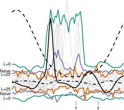
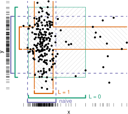
Figure 1: Examples 1 and 2. Please see text for details. LEFT: Local anomalies in time series (solid black line) are easier to spot when computing the confidence area using the proposed method (orange lines) as opposed to existing approaches (green lines). RIGHT: Our approach results in a confidence area (orange “cross”) that is a better representation of the underlying distribution than existing approaches (green rectangle).

The simplest approach to construct multivariate confidence intervals is to compute one-dimensional intervals separately for every variable. While this naive approach satisfies conditions a) and b) above, it is easy to see how it fails in general. Assume, e.g., that we have 10 independently distributed variables, and have computed for each variable a 90% confidence interval. This means that when considering every variable individually, only 10% of the distribution lies outside of the respective interval, as desired. But taken together, the probability that an observation is outside at least one of the confidence intervals is as much as $1-0.9^{10}=65$%. This probability, however, depends strongly on the correlations between the variables. If the variables were perfectly correlated with a correlation coefficient of $\pm 1$, the probability of an observation being outside all confidence intervals would again be 10%. In general the correlation structure of the data affects in a strong and hard-to-predict way on how the naive confidence intervals should be interpreted in a multivariate setting.

Ideally a multivariate confidence area should retain the simplicity of a one-dimensional confidence interval. It should be representable by upper and lower bounds for each variable and the semantics should be the same: each observation is either inside or outside the confidence area, and most observations of a sample should be inside. Particularly important is specifying when an observation in fact is within the confidence area, as we will discuss next.

Confidence areas for time series data have been defined [9, 11] in terms of the minimum width envelope (MWE) problem: a time series is within a confidence area if it is within the confidence interval of every variable. While this has desirable properties, it can, however, result in very conservative confidence areas if there are local deviations from what constitutes “normal” behavior. The definition in [11] is in fact too strict by requiring an observation to be contained in all variable-specific intervals.

Thus, here we propose an alternative way to define the confidence area: a data vector is within the confidence area if it is outside the variable-specific confidence intervals at most $l$ times, where $l$ is a given integer. This formulation preserves easy interpretability: the user knows that any observation within the confidence area is guaranteed to violate at most $l$ variable-specific confidence intervals. In the special case $l=0$, this new definition coincides with the MWE problem [11]. The following examples illustrate further properties and uses of the new definition.

Example 1: local anomalies in time series.

The left panel of Fig. 1 presents a number of time series over $m=80$ time points, shown in light gray, together with three different types of 90% confidence intervals, shown in green, purple and orange, respectively. In this example, “normal” behavior of the time series is exemplified by the black dash-dotted curve that exhibits no noteworthy fluctuation over time. Two other types of time series are shown also in black: a clear outlier (dashed black line), and a time series that exhibits normal behavior most of the time, but strongly deviates from this for a brief moment (solid black line).

In the situation shown, we would like the confidence interval to only show what constitutes “normal” behavior, i.e., not be affected by strong local fluctuations or outliers. Such artifacts can be caused, e.g., by measurement problems, or other types of data corruption. Alternatively, such behavior can also reflect some interesting anomaly in the data generating process, and this should not be characterized as “normal” by the confidence interval. In Fig. 1 (left) the confidence area based on MWE [11], is shown by the green lines; recall the MWE interval corresponds to setting $l=0$. While it is unaffected by the outlier, it strongly reacts to local fluctuations. The naive confidence area, i.e., one where we have computed confidence intervals for every time point individually, is shown in purple. It is also affected by local peaks, albeit less than the $l=0$ confidence area. Finally, the proposed method is shown in orange. The area is computed using $l=25$, i.e., a time series is still within the confidence area as long as it lies outside in at most 25 time points. This variant focuses on what we would expect to be normal behavior in this case. Our new definition of a confidence area is thus nicely suited for finding local anomalies in time series data.

Example 2: representing data distributions.

On the other hand, the right panel of Fig. 1 shows an example where we focus only on the time points $x$ and $y$ as indicated in the left panel. Time point $x$ resides in the region with a strong local fluctuation, while at $y$ there are no anomalies. According to our definition, an observation, in this case an $(x,y)$ point, is within the confidence area if it is outside the variable-specific confidence intervals at most $l$ times. We have computed two confidence areas using our method, one with $l=0$ (green), and another with $l=1$ (orange), as well as the naive confidence intervals (purple).

For $l=0$, we obtain the green rectangle in Fig. 1 (right panel). The variable specific confidence intervals have been chosen so that the green rectangle contains 90% the data and the sum of the widths of the confidence intervals (sides of the rectangle) is minimized. For $l=1$, we obtain the orange “cross” shaped area. The cross shape follows from allowing an observation to exceed the variable specific confidence interval in $l=1$ dimensions. Again, the orange cross contains 90% of all observations, and has been chosen by greedily minimizing the sum of the lengths of the respective variable-specific confidence intervals. It is easy to see that with $l=0$, i.e., when using the MWE method [11], the observations do not occur evenly in the resulting confidence area (green rectangle). Indeed, the top right and bottom right parts of the rectangle are mostly empty. In contrast, with $l=1$, the orange cross shaped confidence area is a much better description of the underlying data distribution, as there are no obvious “empty” parts. Our novel confidence area is thus a better representation of the underlying data distribution than the existing approaches.

Contributions

The basic problem definition we study in this paper is straightforward: for $m$-dimensional data and the parameters $\alpha\in[0,1]$ and integer $l$, find a confidence interval for each of the variables so that the $1-\alpha$ fraction of the observations lie within the confidence area, defined so that the sum of the length of the intervals is minimized, and an observation can break at most $l$ of the variable-specific confidence intervals. We make the following contributions in this paper:

• We formally define the problem of finding a multivariate confidence area, where observations have to satisfy most but not all of the variable-specific confidence intervals.

• We analyze the computational complexity of the problem, and show that it is NP-hard, but admits an approximation algorithm based on a linear programming relaxation.

• We propose two algorithms, which produce good confidence areas in practice.

• We conduct experiments demonstrating various aspects of multivariate confidence intervals.

The rest of this paper is organized as follows: Related work is discussed in Sec. 2. We define the ProbCI and CombCI problems formally in Sec. 3. In Sec. 4 we study theoretical properties of the proposed confidence areas, as well as study problem complexity. Sec. 5 describes algorithms used in experiments in Sec. 6. Finally, Sec. 7 concludes this work.

2 Related work

Confidence intervals have recently gained more popularity, as they convey information both of statistical significance of the result as well as the effect size. In contrast, p-values give information only of the statistical significance: it is possible to have statistically significant results that are meaningless in practice due to the small effect size. The problem has been long and acutely recognized, e.g., in medical research [5]. Some psychology journals have recently banned the use of p-values [18, 16]. The proposed solution is not to report p-values at all, but use confidence intervals instead [14].

Simultaneous confidence intervals for time series data have been proposed [9, 11]. These correspond to the confidence areas in this paper when $l=0$. The novelty here generalization of the confidence areas to allow outlying dimensions ($l>0$), similarly to [17], and the related theoretical and algorithmic contributions, allowing for narrower confidence intervals and in some cases more readily interpretable results. Simultaneous confidence intervals with $l=0$ were in [2, p. 154], and studied [13] by using the most extreme value within a data vector as a ranking criterion. Another examples of $l=0$ type procedures include [12, 15]. In the field of information visualization and the visualization of time series confidence areas have been used extensively; see [1] for a review. An interesting approach is to construct simultaneous confidence regions by inverting statistical multiple hypothesis testing methods, see e.g., [6].

The approach presented in this paper allows some dimensions of an observation to be partially outside the confidence area. This is in the same spirit—but not equivalent—to false discovery rate (FDR) in multiple hypothesis testing, which also allows a controlled fraction of positives to be “false positives”. In comparison, the approach in [11] is more akin to family-wise error rate (FWER) that controls the probability of at least one false discovery.

3 Problem definition

A data vector $x$ is a vector in ${\mathbb{R}}^{m}$ and $x(j)$ denotes the value of $x$ in $j$th position. Let matrix $X\in{\mathbb{R}}^{n\times m}$ be a dataset of $n$ data vectors $x_{1},\ldots,x_{n}$, i.e. rows of $X$. We start by defining the confidence area, its size, and the envelope for a dataset $X$.

Definition 3.1.

Given $X\in{\mathbb{R}}^{n\times m}$, a confidence area for $X$ is a doublet of vectors $(x_{l},x_{u})$, $x_{l},x_{u}\in{\mathbb{R}}^{m}$ composed of lower and upper bounds satisfying $x_{l}(j)\leq x_{u}(j)$ for all $j$, respectively. The size of the confidence area is $A=\sum_{j=1}^{m}{w(j)}$, where $w(j)=x_{u}(j)-x_{l}(j)$ is the width of the confidence interval w.r.t. $j$th position. The envelope of $X$ is a confidence area denoted by $\operatorname{env}(X)=(x_{l},x_{u})$, where $x_{l}(j)=\min_{i=1}^{n}{x_{i}(j)}$ and $x_{u}(j)=\max_{i=1}^{n}{x_{i}(j)}$.

We define the error of the confidence area as the number of outlying data vectors as follows.

Definition 3.2.

Let $x$ be a data vector in $\mathbb{R}^{m}$ and $(x_{l},x_{u})$ a confidence area. The error of $x$ given the confidence area is defined as

$$V(x\mid x_{u},x_{l})=\sum_{j=1}^{m}\operatorname{I}\left[x(j)<x_{l}(j)\vee x_{u}(j)<x(j)\right].$$

The indicator function $\operatorname{I}[\Box]$ is unity if the condition $\Box$ is satisfied and zero otherwise.

The main problem in this paper is as follows.

Problem 3.1 (ProbCI).

Given $\alpha\in[0,1]$, an integer $l$, and a distribution $F$ over $\mathbb{R}^{m}$, find a confidence area $(x_{l},x_{u})$ that minimizes $\sum_{j=1}^{m}w(j)$ subject to constraint

(3.1) $$\Pr_{x\sim F}\left[V(x\mid x_{u},x_{l})\leq l\right]\geq 1-\alpha.$$

For this problem definition to make sense, the variables or at least their scales must be comparable. Otherwise variables with high variance will dominate the confidence areas. Therefore, some thinking and a suitable preprocessing, such as normalization of variables, should be applied before solving for the confidence area and interpreting it.

The combinatorial problem is defined as follows.

Problem 3.2 (CombCI).

Given integers $k$ and $l$, and $n$ vectors $x_{1},\ldots,x_{n}$ in $\mathbb{R}^{m}$, find a confidence area $(x_{l},x_{u})$ by minimizing $\sum_{j=1}^{m}w(j)$ subject to constraint

(3.2) $$\sum_{i=1}^{n}\operatorname{I}\left[V(x_{i}\mid x_{u},x_{l})\leq l\right]\geq n-k.$$

Any confidence area satisfying (3.2) is called a $(k,l)$-confidence area. In the special case with $l=0$, Problems 3.1 and 3.2 coincide with the minimum width envelope problem from [11]. The problem definition with non-vanishing $l$ is novel to best of our knowledge. The relation of Problems 3.1 and 3.2 is as follows.

Definition 3.3.

Problems 3.1 and 3.2 match for a given data from distribution $F$ and parameters $\alpha$, $k$, and $l$, if a solution of Problem 3.2 satisfies Eq. (3.1) with equality for a previously unseen test data from distribution $F$.

We can solve Problem 3.1 by solving Problem 3.2 with different values of $k$ to find a $k$ that matches the given $\alpha$, as done in Sec. 6.2 or [11].

4 Theoretical observations

4.1 Confidence areas for uniform data

It is instructive to consider the behavior of Problem 3.1 with the uniform distribution $F_{unif}=U(0,1)^{m}$. We show that a solution may contain very narrow confidence intervals and discuss the required number of data vectors to estimate a confidence area with a desired level of $\alpha$.

Consider Problem 3.1 in a simple case of two-dimensional data with $m=2$, $l=1$, and $\alpha=0.1$. In this case an optimal solution to Problem 3.1 is given by confidence intervals with $w(1)=0.9$ and $w(2)=0$, resulting in the size of confidence area of $\sum_{j=1}^{2}{w(j)}=0.9$. A solution with confidence intervals of equal width, i.e., $w(1)=w(2)=0.68$ would lead to substantially larger area of $1.37$. As this simple example demonstrates, if data is unstructured or if some of the variables have unusually high variance, we may obtain solutions where some of the confidence intervals are very narrow. In the case of uniform distribution the choice of variables with zero width confidence intervals is arbitrary: e.g., in the example above we could as well have chosen $w(1)=0$ and $w(2)=0.9$. Such narrow intervals are not misleading, because they are easy to spot: for a narrow interval—such as the one discussed in this paragraph—only a small fraction of the values of the variable lie within it. In real data sets with non-trivial marginal distributions and correlation structure the confidence intervals are often of roughly similar width.

Next we consider the behavior of the problem at the limit of high-dimensional data.

Lemma 4.1.

The solution with confidence intervals of equal width $w=w_{j}=x_{u}(j)-x_{l}(j)$ corresponds to $\alpha$ of

(4.3) $$\alpha=1-BC(l,m,w),$$

where $BC(l,m,w)=\sum_{j=0}^{l}\binom{m}{j}(1-w)^{j}w^{m-j}$ is the cumulative binomial distribution.

Lemma 4.2.

If $n$ vectors are sampled from $F_{unif}=U(0,1)^{m}$ then the expected width of the envelope for each variable is $w=\frac{n-1}{n+1}$. The probability of more than $l$ variables from a vector from $F_{unif}$ being outside the envelope is given by Eq. (4.3) with $w=\frac{n-1}{n+1}$.

One implication of Lemma 4.2 is that there is a limit to the practical accuracy that can be reached with a finite number of samples. The smallest $\alpha$ we can hope to realistically reach is the one implied by the envelope of the data, unless we make some distributional assumptions of the shape of the distribution outside the envelope. Conversely, the above lemmas define a minimum number of samples needed for uniform data to find the confidence area for a desired level of $\alpha$.

In the case of $l=0$ to reach the accuracy of $\alpha$, we have $w^{m}\approx 1-\alpha$, or $n\approx-2m/\log{\left(1-\alpha\right)}\approx 2m/\alpha$, where we have ignored higher order terms in $1/m$ and $\alpha$. For a typical choice of $\alpha=0.1$ and $m=100$ this would imply that at least $n\approx 2000$ data vectors are needed to estimate the confidence area; the number of data vectors needed increases linearly with the dimensionality $m$.

On the other hand, for a given $\beta\in]0,1[$, if we let $l=\lfloor\beta m\rfloor$, a solution where the width of the envelope is $w\approx 1-\beta$ is asymptotically sufficient when the dimensionality $m$ is large, in which case the number of data vectors required is $n\approx 2/\beta$. For a value of $\beta=0.1$ only $n\approx 20$ data vectors would therefore be needed even for large $m$. As hinted by the toy example in Fig. 1, a non-vanishing parameter $l$ leads at least in this example to substantially narrower confidence intervals and, hence, make it possible to compute the confidence intervals with smaller data sets.

4.2 Complexity and approximability

We continue by briefly addressing the computational properties of the CombCI problem. The proofs are provided in the appendix.

Theorem 4.1.

CombCI is NP-hard for all $k$.

For $k>0$ the result directly follows from [11, Theorem 3], and for $k=0$ and $l>0$ a reduction from Vertex-Cover can be used.

Now, there exists a polynomial time approximation algorithm for solving a variant of CombCI in the special case of $k=0$. In particular, we consider here a one-sided confidence area, defined only as the upper bound $x_{u}$, the lower bound $x_{l}$ is assumed to be fixed, e.g., at zero, or any other suitable value. This complements the earlier result that the complement of the objective function of CombCI is hard to approximate for $k>0$ and $l=0$ [11, Theorem 3].

Theorem 4.2.

There is a polynomial time $(l+1)$ approximation algorithm for the one-sided CombCI problem with $k=0$.

The proof uses a linear programming relaxation of an integer linear program corresponding to the $k=0$ variant of the one-sided CombCI and the approximation ratio obtained from the solution given by the relaxation.

Finding a bound that does not depend on $l$ is an interesting open question, as well as extending the proof to the two-sided CombCI. It is unlikely that the problem admits a better approximation bound than $2$, since this would immediately result in a new approximation algorithm for the Vertex-Cover problem. This is because in the proof of Theorem 4.2 we describe a simple reduction from Vertex-Cover to CombCI with $l=1$ and $k=0$. This reduction preserves approximability, as it maps the Vertex-Cover instance to an instance of our problem in a straightforward manner. For Vertex-Cover it is known that approximation ratios below $2$ are hard to obtain in the general case. Indeed, the best known bound is equal to $2-\Theta(1/\sqrt{\log|V|})$ [8].

5 Algorithms

We present two algorithms for $(k,l)$-confidence areas.

5.1 Minimum intervals (mi)

Our first method is based on minimum intervals. A standard approach to define a confidence interval for univariate data is to consider the minimum length interval that contains $(1-a)$% of the observations. This can be generalized for multivariate data by treating each variable independently, i.e., for a given $a$, we set $x_{l}(j)$ and $x_{u}(j)$ equal to lower and upper limit of such a minimum length interval for every $j$. The mi algorithm solves the CombCI problem for given $k$ and $l$ by adjusting the parameter $a$ such that the resulting $(x_{u},x_{l})$ satisfies the constraint in Eq. (3.2) in the training data set. The resulting confidence area may have a larger size than the optimal solution, since all variables use the same $a$. Note that the mi solution differs from the naive solution mentioned in the introduction because the naive solution does not adjust $a$ but simply sets it to $a=k/n$. The time complexity of mi with binomial search for correct $a$ is $O(mn\log{k}\log{n})$.

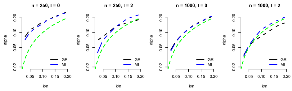
Figure 2: Comparison of $k/n$ used when fitting the confidence interval on training data and the observed level of $\alpha$ in a separate test data. Both data are normal with $m=10$, $n_{test}=1000$, $n_{train}=\{250,1000\}$ and $l=\{0,2\}$. The dashed green line indicates $k/n=\alpha$. Shown are the averages over 25 independent trials over different randomly generated training and test instances. Note the log-scale on the vertical axis.

5.2 Greedy algorithm (gr)

Our second method is a greedy algorithm. The greedy search could be done either bottom-up (starting from an empty set of included data vectors and then adding $n-k$ data vectors) or top-down (starting from $n$ data vectors and by excluding $k$ data vectors). Since typically $k$ is smaller than $n-k$ we will consider here a top-down greedy algorithm.

The idea of the greedy algorithm is to start from the envelope of whole data and sequentially find $k$ vectors to exclude by selecting at each iteration the vector whose removal reduces the envelope the largest amount. In order to find the envelope wrt. the relaxed condition allowing $l$ positions from each vector to be outside, at each iteration the set of included data points needs to be (re)computed. This is done by implementing a greedy algorithm solving the CombCI problem for $k=0$. Here one removes individual points that result in maximal decrease in the envelope size so that at most $l$ points from each data vector are be removed, thus obtaining the envelope wrt. the $l$ criterion. After this envelope has been computed, the data vector whose exclusion yields a maximal decrease in the size of the confidence area is excluded. For this, a slightly modified variant of the greedy MWE algorithm from [11] with $k=1$ is used. After $k$ data vectors have been excluded, the final set of points included in the envelope is returned. The time complexity of gr is $O(mkn\log{n})$.

6 Empirical evaluation

We present here empirical evaluation of the algorithms. In the following mi and gr refer to the Minimum intervals and Greedy algorithm, respectively.

6.1 Datasets

We make experiments using various datasets that reflect different properties of interest from the point of view of fitting confidence areas. In particular, we want to study the effects of correlation (autocorrelation in the case of time-series or regression curves), number of variables, and distributional qualities.

• Artificial data. We use artificial multivariate (i.i.d. variables) datasets sampled from the uniform distribution (in the interval $[0,1]$), the standard normal distribution, and the Cauchy distribution (location parameter $0$, scale parameter $\gamma=2$), with varying $n$ and $m$ to study some theoretical properties of multivariate confidence areas.

• Kernel regression data. We use the Ozone and South African heart disease (SA heart) datasets (see, e.g., [4]) to compute confidence areas for bootstrapped kernel regression estimates. We use a simple Nadaraya-Watson kernel regression estimate to produce the vectors $X$, and fit confidence intervals to these using our algorithms. By changing the number of bootstrap samples we can vary $n$, and by altering the number of points in which the estimate is computed we can vary $m$.

• Stock market data. We obtained daily closing prices of $n=400$ stocks for years 2011–2015 ($m=1258$ trading days). The time-series are normalized to reflect the absolute change in stock price with respect to the average price of the first five trading days in the data. The data is shown in Fig. 5.

6.2 Finding the correct $\mathbf{k}$

Our algorithms both solve the CombCI problem (Problem 3.2) in which we must specify the number of vectors $k$ that are allowed to violate the confidence area. To obtain a matching $\alpha$ in ProbCI (Definition 3.3) we must choose the parameter $k$ appropriately. We study here how this can be achieved.

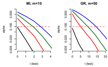
Figure 3: Effect of the value of $l_{\operatorname{test}}$ on the observed $\alpha$ for different values of $l_{\operatorname{train}}$. On the left $l_{\operatorname{train}}$ is equal to $0$ (black), $1$ (red), $2$ (green) and $3$ (blue), while on the right $l_{\operatorname{train}}$ is $0$ (black), $5$ (red), $10$ (green), and $15$ (blue). In every case the confidence area was trained to have $\alpha=0.1$ for the given $l_{\operatorname{train}}$.

Fig. 2 shows $\alpha$ as a function of $k/n$ in data with $m=10$ independent normally distributed variables for four combinations of $n$ and $l$. The dashed green line shows the situation with $k/n=\alpha$. (This is a desirable property as it means fine-tuning $k/n$ is not necessary to reach some particular value of $\alpha$.) We observe from Fig. 2 that when the data is relatively small ($n=250$), for a given $k/n$ both gr as well as mi tend to find confidence areas that are somewhat too narrow for the test data leading to $\alpha>k/n$. To obtain some particular $\alpha$, we must thus set $k/n$ to a lower value. For example, with $n=250$ and $l=0$, to have $\alpha=0.1$ we must let $k/n=0.05$. As the number of training examples is increased to $n=1000$, we find that both algorithms are closer to the ideal situation of $k/n=\alpha$. Interestingly, this happens also when when $l$ increases from $l=0$ to $l=2$. The relaxed notion of confidence area we introduce in this paper is thus somewhat less prone to overfitting issues when compared against the basic confidence areas with $l=0$ of [11]. On the other hand, for $n=1000$ we also observe how gr starts to “underfit” as $k/n$ increases, meaning that we have $\alpha<k/n$. Errors in this direction, however, simply mean that the resulting confidence area is conservative and will satisfy the given $k/n$ by a margin.

The dependency between $k/n$ and $\alpha$ and other observations made above are qualitatively identical for uniform and Cauchy distributed data (not shown).

6.3 Effect of $l$ on $\alpha$ in test data

Note that the value of $\alpha$ that we compute for a given confidence area also depends on the value of $l$ used when evaluating. We continue by showing how $\alpha$ depends on the value of $l$ used when evaluating the confidence area on test data. In this experiment we train confidence areas using the Ozone data (with $n=500$ and $m=10$ or $m=50$) and adjust $k/n$ so that we have $\alpha=0.1$ for a given value of $l_{\operatorname{train}}$, where $l_{\operatorname{train}}\in\{0,0.1m,0.2m,0.3m\}$ is the parameter given to our algorithms (mi, gr) to solve Prob. 3.2. Then we estimate $\alpha$ for all $l_{\operatorname{test}}\in\{1,\ldots,m\}$ using Eq. (3.1) and previously unseen test data set.

Results are shown in Fig. 3. We find that in every case the line for a given value of $l_{\operatorname{train}}$ intersects the thin dashed (red) line (indicating $\alpha=0.1$) at the correct value $l_{\operatorname{test}}=l_{\operatorname{train}}$. More importantly, however, we also find that $l_{\operatorname{test}}$ has a very strong effect on the observed $\alpha$. This means that if we relax the condition under which an example still belongs in the confidence area (i.e., increase $l_{\operatorname{test}}$), $\alpha$ drops at a very fast rate, meaning that a confidence area trained for a particular value of $l_{\operatorname{train}}$, will be rather conservative when evaluated using $l_{\operatorname{test}}>l_{\operatorname{train}}$. Obviously the converse holds as well, i.e., when $l_{\operatorname{test}}<l_{\operatorname{train}}$, the confidence area will become much too narrow very fast. This implies that $l_{\operatorname{train}}$ should be set conservatively (to a low value) when it is important to control the false positive rate, e.g., when the “true” number of noisy dimensions is unknown.

6.4 Algorithm comparison

Next we briefly compare the mi and gr algorithms in terms of the confidence area size (given as $A/m$, where $m$ is the number of variables) and running time $t$ (in seconds). Results for artificial data sets as well as the two regression model data are shown in Table 1. The confidence level (in test data) was set to $\alpha=0.1$ in every case, and all training data had $n=500$ examples. All numbers are averages of 25 trials. We can observe, that mi tends to produce confidence areas that are consistently somewhat smaller than those found by gr. Also, mi is substantially faster, albeit our implementation of gr is by no means optimized. Finally, the $k/n$ column shows the confidence level that was used when fitting the confidence area to obtain $\alpha=0.1$. Almost without exception, we have $k/n<\alpha$ for both algorithms, with mi usually requiring a slightly larger $k$ than gr. Also worth noting is that for extremely skewed distributions, e.g., Cauchy, the confidence area shrinks rapidly as $l$ is increased from zero.

			mi			gr
dataset	$l$	$m$	$A/m$	$t$	$k/n$	$A/m$	$t$	$k/n$
unif	0	10	1.0	0.1	0.06	1.0	0.7	0.07
unif	2	10	0.9	0.2	0.08	0.9	14.0	0.11
unif	10	100	0.9	0.7	0.05	0.9	32.1	0.03
unif	50	500	0.9	2.1	0.03	0.9	220.2	0.03
norm	0	10	5.1	0.1	0.07	5.3	0.8	0.07
norm	2	10	3.2	0.2	0.09	3.2	12.0	0.09
norm	10	100	3.6	0.8	0.06	3.6	33.1	0.03
norm	50	500	3.5	2.1	0.03	3.5	209.7	0.03
Cauchy	0	10	262.3	0.1	0.08	325.1	0.7	0.07
Cauchy	2	10	21.8	0.1	0.09	25.6	10.7	0.08
Cauchy	10	100	36.8	0.7	0.07	38.5	31.4	0.03
Cauchy	50	500	30.5	2.2	0.05	31.5	203.3	0.03
ozone	0	10	5.1	0.1	0.08	5.1	0.8	0.07
ozone	2	10	3.4	0.1	0.09	3.5	9.0	0.09
ozone	5	50	4.2	0.3	0.09	4.3	11.4	0.05
ozone	15	50	3.0	0.3	0.09	3.1	48.6	0.06
SA heart	0	10	5.3	0.1	0.06	5.4	0.7	0.06
SA heart	2	10	3.3	0.2	0.08	3.7	15.5	0.14
SA heart	5	50	4.3	0.2	0.07	4.5	8.6	0.04
SA heart	15	50	2.9	0.3	0.08	3.3	66.7	0.06

Table 1: Comparison between mi and gr.

Figure 4: Using gr and mi on bootstrapped kernel regression estimates ($n=250$, $m=30$, $l\in\{0,5\}$). Top: Probability of coronary heart disease as a function of systolic blood pressure in the SA heart data. Bottom: Ozone level as a function of observed radiation.

6.5 Application to regression analysis

We can model the accuracy of an estimate given by a regression model by resampling the data points, e.g., by the bootstrap method, and then refitting the model for each of the resampled data sets [3]. The estimation accuracy or spread of values for a given independent variable can be readily visualized using confidence intervals.

Fig. 4 shows examples of different confidence intervals fitted to bootstrapped kernel regression estimates on two different datasets using both $l=0$ and $l=5$ ($n=250$ and $m=30$). In both cases $k$ was adjusted so that $\alpha=0.1$ in a separate test data. We find that qualitatively there is very little difference between mi and gr when $l=5$. For $l=0$, gr tends to produce a somewhat narrower area. In general, this example illustrates the effect of $l$ on the resulting confidence area in visual terms. By allowing the examples to lie outside the confidence bounds for a few variables ($l=5$) we obtain substantially narrower confidence areas that still reflect very well the overall data distribution.

6.6 Stock market data

The visualization for the stock market data of Fig. 5 has been constructed using gr algorithm with parameters $k=40$ and $l=125$. The figure shows in yellow the stocks that are clearly outliers and among the $k=40$ anomalously behaving observations ignored in the construction of the confidence area. The remaining $n-k=360$ stocks (shown in blue) remain within the confidence area at least $\frac{m-l}{m}=90$% of the time. However, they are allowed to deviate from the confidence area 10% of the time. Fig. 5 shows several such stocks, one of them highlighted with red. By allowing these excursions, the confidence area is smaller and these potentially interesting deviations are easy to spot. E.g., the red line represents Mellanox Technologies and market analyses from fall 2012 report the stock being overpriced at that time. The black line in Fig. 5 represents Morningstar, an example staying inside the confidence area. If we do not allow any deviations outside the confidence intervals, i.e., we set $l=0$, then the confidence area will be larger and such deviations might be missed.

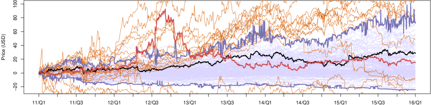
Figure 5: Visualization of the relative closing values of 400 stocks from Jan. 2011 to Dec. 2015 (1258 days) compared to the starting days. The confidence area with parameters $k=40$ and $l=125$ is shown with blue lines. An example of a valuation of a stock that temporarily deviates (in less than $l$ time points) from the confidence area is shown in red, and an example of a valuation for a stock observing “normal” development is shown in black.

7 Concluding remarks

The versatility of confidence intervals stems from their simplicity. They are easy to understand and to interpret, and therefore often used in presentation and interpretation of multivariate data. The application of confidence intervals to multivariate data is, however, often done in a naive way, disregarding effects of multiple variables. This may lead to false interpretations of results if the user is not being careful.

In this paper we have presented a generalization of confidence intervals to multivariate data vectors. The generalization is simple and understandable and does not sacrifice the interpretability of one-dimensional confidence intervals. The confidence areas defined this way behave intuitively and offer insight into the data. The problem of finding confidence areas is computationally hard. We present two efficient algorithms to solve the problem and show that even a rather simple approach (mi) can produce very good results.

Confidence intervals are an intuitive and useful tool for visually presenting and analyzing data sets, spotting trends, patterns, and outliers. The advantage of confidence intervals is that they give at the same time information about both the statistical significance of the result and size of the effect. In this paper, we have shown several examples demonstrating the usefulness of multivariate confidence intervals, i.e. confidence areas.

In addition to visual tasks, the confidence intervals can also be used in automated algorithms as a simple and robust distributional estimators. As the toy example of Fig. 1 shows, the confidence areas with $l>0$ can be a surprisingly good distributional estimator, if data is sparse, i.e., a majority of variables is close to the mean and in each data vector only a small number of variables have significant deviations from the average.

With p-values there are established procedures to deal with multiple hypothesis testing. Indeed, a proper treatment of the multiple comparisons problem is required, e.g., in scientific reporting. Our contribution to the discussion about reporting scientific results is to point out that it is indeed possible to treat multidimensional data with confidence intervals in a principled way.

Appendix A Appendix

A.1 Proof of Theorem 4.1

The case of $k>0$ follows directly from [11, Theorem 3]. In the case $k=0$ we use a reduction from Vertex-Cover. In the Vertex-Cover problem we are given a graph $G$, and an integer $K$, and the task is to cover every edge of $G$ by selecting a subset of vertices of $G$ of size at most $K$. A reduction from Vertex-Cover to the CombCI problem maps every edge $e=(a,b)$ of the input graph $G$ into the vector $x_{e}$, where $x_{e}(a)=x_{e}(b)=1$, and $x_{e}(w)=0$ when $w\not\in\{a,b\}$. Furthermore, we add two vectors $x_{a}$ and $x_{b}$ which satisfy $x_{a}(1)=x_{b}(2)=-m-1$ and which have a value of zero otherwise. Moreover, we set $k=0$ and $l=1$.

For the optimal confidence area, we must allow the first element of vector $a$ and the second element of vector $b$ be outside the confidence area, resulting to a lower bound $x_{l}(j)=0$ for all $j$. Thus, it suffices to consider a variant of the problem where the input vectors $x_{i}$ are constrained to reside in $\{0,1\}^{m}$ and to seek an upper bound $x_{u}\in\{0,1\}^{m}$. To minimize the size of the confidence area we need to minimize the number of $1$s in $x_{u}$. We consider a decision variant of the CombCI problem where we must decide if there exists an $x_{u}$ with $\sum_{j}x_{u}(j)\leq K$ for a given integer $K$. An optimal vertex cover is obtained simply by selecting the vertices $j$ with $x_{u}(j)=1$ in the optimal upper bound $x_{u}$.

A.2 Proof of Theorem 4.2

To prove Theorem 4.2 we use a linear programming relaxation of an integer linear program (ILP) corresponding to the $k=0$ variant of the one-sided CombCI which we define as follows. Let $X$ be a matrix representing the data vectors $x_{1},\ldots,x_{n}$. For the moment, consider the $j$th position of every vector $x_{i}$ in $X$, and let this be sorted in decreasing order of $x_{i}(j)$. Let $i^{\prime}$ denote the vector that follows vector $i$ in this sorted order. Moreover, at every position $j$ we only consider vectors that are strictly above the lower bound $x_{l}(j)$.

The ILP we define uses binary variables $q$ to express whether a given vector is inside the one-sided confidence area. We have $q_{i}(j)=1$ when vector $i$ is contained in the confidence area at position $j$, and $q_{i}(j)=0$ otherwise.

To compute the size of the confidence area, we introduce a set of coefficients, denoted by $\Delta$. We define $\Delta_{i}(j)=x_{i}(j)-x_{i^{\prime}}(j)$ as the difference between the values of vectors $i$ and $i^{\prime}$ at position $j$. For the vector $i$ that appears last in the order, i.e., there is no corresponding $i^{\prime}$, we let $\Delta_{i}(j)=x_{i}(j)-x_{l}(j)$, where $x_{l}(j)$ is the value of the lower side of the confidence interval at position $j$. Using this, we can write the difference between the largest and smallest value at position $j$ as the sum $\sum_{i=1}^{n}\Delta_{i}(j)$, and the size of the envelope that contains all of $X$ is equal to $\sum_{j=1}^{m}\sum_{i=1}^{n}\Delta_{i}(j)$.

Now, given a feasible assignment of values to $q$, i.e., an assignment that satisfies the constraints that we will define shortly, we can compute the size of the corresponding one-sided confidence area using the sum $\sum_{i=1}^{n}\sum_{j=1}^{m}q_{i}(j)\Delta_{i}(j)$. This is the objective function of the ILP.

We continue with discussing the constraints. Recall that $i^{\prime}$ denotes the vector that follows vector $i$ when the vectors are sorted in decreasing order of their value at position $j$. First, since every vector $i$ may violate the confidence area at most at $l$ positions, we must make sure that $\sum_{j=1}^{m}q_{i}(j)\geq m-l$ holds for every $i$. Moreover, observe that if the vector at position $i$ is within the upper bound at position $j$, i.e., we have $q_{i}(j)=1$, the vector $i^{\prime}$ must be inside the upper bound at position $j$ as well, since $x_{i}(j)\geq x_{i^{\prime}}(j)$. However, if the vector $i^{\prime}$ is below the upper bound, this does not imply anything for vector $i$. Therefore, we must have $q_{i}(j)\leq q_{i^{\prime}}(j)$ for all $i$ and $j$.

The resulting ILP is as follows:

(A.4) $$\min\;\sum_{i,j}q_{i}(j)\Delta_{i}(j)$$ st.

(A.5) $$\sum_{j=1}^{m}q_{i}(j) \geq m-l\;\;\forall i$$

(A.6) $$q_{i^{\prime}}(j)-q_{i}(j) \geq 0\;\;\forall i,j$$

(A.7) $$q_{i}(j) \in \{0,1\}\;\;\forall i,j.$$

There are at most $nm$ variables and $nm+n$ constraints in total in addition to the binary constraints. A relaxed version of this ILP is otherwise equivalent, but allows all variables to take fractional values in the interval $[0,1]$. We use standard techniques to design an approximation algorithm for the one-sided CombCI problem (with $k=0$) as follows. The algorithm first computes (in polynomial time using a suitable LP solver) the optimal fractional solution, denoted $q^{*}$, and then rounds this to an integer solution using a simple threshold value. We must select the threshold so that the resulting integer solution is guaranteed to be feasible for the original ILP. We define the rounding procedure as follows:

(A.8) $$\bar{q}_{i}(j)=\begin{cases}1&\text{if }q_{i}(j)^{*}\geq\frac{1}{l+1},\\ 0&\text{otherwise}.\end{cases}$$

The threshold value we use is thus $1/(l+1)$. To prove that the algorithm is correct, we must show (i) that the rounding procedure results in a solution where every vector $i$ is outside the confidence area at most $l$ times, and (ii) that there are no “holes” in the solution, meaning that if $\bar{q}_{i}(j)=1$, then $\bar{q}_{i^{\prime}}(j)$ must be equal to $1$ as well. We start with this latter property.

Lemma A.1.

Consider position $j$, and let all vectors be sorted in decreasing order of $x_{i}(j)$. This order results in a monotonically increasing sequence of $q_{i}(j)^{*}$ values.

Proof.

The proof is a simple observation that since Equation (A.6) holds for any feasible solution, we must have $q_{i^{\prime}}(j)^{*}\geq q_{i}(j)^{*}$ for every $i$ and $j$. ∎

This means that if the rounding procedure of Equation (A.8) sets $\bar{q}_{i}(j)=1$, we must have $\bar{q}_{i^{\prime}}(j)=1$ as well. The result is also guaranteed to include every vector $i$ within the confidence area at least $m-l$ times.

Lemma A.2.

The rounding scheme of Equation (A.8) gives a solution $\bar{q}$ that satisfies the constraint of Equation (A.5) for all $i$.

Proof.

We must find a worst-case distribution of values in $q_{i}^{*}$ that requires a very small threshold value so that the rounded variables satisfy the constraint. Suppose that there are $m-l-1$ ones in $q_{i}^{*}$. Since the total sum of all elements in $q_{i}^{*}$ is at least $m-l$, the remaining $l+1$ items must sum to $1$. The worst-case situation happens when all of the remaining $l+1$ items are equal to $1/(l+1)$. By selecting this as the threshold value, we are guaranteed to satisfy the constraint. ∎

Next, we consider the approximation ratio of the solution given by $\bar{q}$. The proof follows standard approaches.

Lemma A.3.

The cost of the rounded solution $\bar{q}$ is at most $(l+1)$ times the optimal solution to the original ILP.

Proof.

By the definition of $\bar{q}$ in Equation (A.8), we must have $\bar{q}_{i}(j)\leq(l+1)q_{i}(j)^{*}$. This implies that

$$\sum_{i,j}\bar{q}_{i}(j)\Delta_{i}(j)\leq(l+1)\sum_{i,j}q_{i}(j)^{*}\Delta_{i}(j).$$

The cost of $\bar{q}$ is thus at most $(l+1)$ times the cost of the optimal fractional LP, which lower bounds the optimal cost of the ILP. ∎

Now, using Lemmas A.1, A.2, and A.3 together, we have an algorithm that implies Theorem 4.2.

Algorithm A.1: Greedy algorithm, top-down.

1:  input: dataset $X\in\mathbb{R}^{N\times M}$, integers $K$,$L$

2:  output: $Z\in\{0,1\}^{N\times M}$ indicating included points

3:  $I\leftarrow\{1,\ldots,N\}$

4:  $Z\leftarrow$zeros$(N,M)$

5:  for $k=1\ldots K$ do

6:     $R\leftarrow$FindEnvelope$(X,I,L)$

7:     $I\leftarrow I\setminus\{$ExcludeObservation$(X,R)\}$

8:  end for

9:  $R\leftarrow$FindEnvelope$(X,I,L)$

10:  $Z(i,j)\leftarrow 1$ for all points $(i,j)$ included in $R$

11:  return  $Z$

A.3 Greedy algorithm

The idea of the greedy algorithm, presented in Algorithm A.1, is to start from the whole data envelope and sequentially find $k$ vectors to exclude by selecting at each iteration the vector whose removal reduces the envelope the largest amount. In order to find the envelope wrt. the relaxed condition that allows $l$ positions from each vector to be outside, at each iteration the set of included data points needs to be (re)computed (line 6). This is realized in function FindEnvelope (details presented in Algorithm A.2), which essentially implements a greedy algorithm solving the CombCI problem for $k=0$. After the envelope has been computed, the data vector whose exclusion yields a maximal decrease in the size of the confidence area is excluded. The function ExcludeObservation (details presented in Algorithm A.3) is a variant of as the greedy MWE algorithm from [11] with $k=1$, and with the ordering structure $R$ provided. After $k$ data vectors have been excluded FindEnvelope is called for the final set of data vectors in line 9 and matrix indicating included points is returned.

Algorithm A.2: FindEnvelope$(X,I,L)$

1:  input: dataset $X\in\mathbb{R}^{N\times M}$, $I\subseteq 2^{N}$, integer $L$

2:  output: ordering structure $R$

3:  rmd$\leftarrow$zeros($N$)

4:  $U\leftarrow$list()

5:  $R\leftarrow$ordering structure for observations in $X[I,:]$

6:  for $j=1\ldots M$ do

7:     for $b=0\ldots 1$ do

8:        $v\leftarrow|X[$1st$(R,j,b),j]-X[$2nd$(R,j,b),j]|$

9:        $U$.add(key=$v$, col=$j$, up=$b$)

10:     end for

11:  end for

12:  $G\leftarrow$priorityQueue$(U)$

13:  while $G\neq\emptyset$ and $\sum_{i}$rmd$(i)<N\cdot L$ do

14:     $(v,j,b)\leftarrow$getMaximumElement($G$)

15:     $i\leftarrow$1st$(R,j,b)$

16:     if rmd$(i)<L$ then

17:        $R\leftarrow$remove1st$(R,j,b)$

18:        rmd($i$)$\leftarrow$rmd($i$)+1

19:        $v\leftarrow|X[$1st$(R,j,b),j]-X[$2nd$(R,j,b),j]|$

20:        $G$.add(key=$v$, col=$j$, up=$b$)

21:     end if

22:  end while

23:  return  $R$

The function FindEnvelope, presented in Algorithm A.2, identifies which $l$ points from each data vector to leave outside of the confidence area in order to obtain a confidence area of minimal size. To efficiently maintain information about the ordering of the values in columns an ordering structure $R$ is used (line 5). Each element of $R$ is a doubly-linked list $R_{j}$ storing the ordering information for column $j$, with the first element corresponding to the row index of the smallest element in $X[:,j]$. Several functions are associated with $R$. The function 1st$(R,j,b)$ returns the row index of the smallest ($b=0$) or the largest ($b=1$) value for column $j$ in $X$, and, similarly, function 2nd$(R,j,b)$ returns the row index of the second smallest or the second largest value. Furthermore, function remove1st$(R,j,b)$ removes the first ($b=0$) or the last element ($b=1)$ of $R_{j}$. Lines 6–12 initialize a priority queue $G$ maintaining a list of candidate points for exclusion along with the respective gains, i.e., reductions of confidence area.

The main part of the search for the points to exclude from the relaxed confidence area is the while-loop in lines 13–22. At each iteration the point $x^{\star}$ leading to maximal decrease in the size of the confidence area is excluded, if less than $l$ elements have already been excluded from the data vector in question. The loop terminates when there are no positions left in which the point with an extreme value can be excluded without breaking the vector-wise constraints.

Our approach in the function ExcludeObservation, presented in Algorithm A.3, is similar to that in [11, Algorithm 1], i.e., the index of observation to remove is the one that results in the maximal decrease in the envelope size wrt. the current one.

Algorithm A.3: ExcludeObservation$(X,R)$

1:  input: dataset $X\in\mathbb{R}^{N\times M}$, ordering structure $R$

2:  output: index of observation to exclude $i$

3:  Create hash table $\Delta U$ s.t. a query with previously unused key returns value of zero

4:   $A\leftarrow\emptyset$

5:  for $j=1\ldots M$ do

6:     for $b=0\ldots 1$ do

7:        $\Delta U[$1st$(R,j,b)]\leftarrow\Delta U[$1st$(R,j,b)]$

8:                  $+|X[$1st$(R,j,b),j]-X[$2nd$(R,j,b),j]|$

9:        $A\leftarrow A\cup\{$1st$(R,j,b)\}$

10:     end for

11:  end for

12:  return  arg max${}_{a\in A}\Delta U[a]$

Notice that for $l=0$ it is computationally more efficient to use the greedy algorithm from [11], as in that case there is no need to update the set of data vectors included in the envelope for each iteration over $k$ as done in Algorithm A.1.

The greedy algorithm performs well in practice, although it does not provide approximation guarantees. Consider, e.g., a setting with $n=5$, $m=2$, $k=0$, and $l=1$ and a data matrix $X$ such that

$$X^{T}=\left(\begin{array}[]{ccccc}0&2\epsilon&4\epsilon&5\epsilon&7\epsilon\\ 3\epsilon&2\epsilon&0&1&1-2\epsilon\end{array}\right)$$

with $\epsilon$ arbitrary small. The optimal solution is given by

$$Z_{\mathsf{opt}}^{T}=\left(\begin{array}[]{ccccc}0&0&1&1&1\\ 1&1&0&0&0\end{array}\right)$$

and has a cost $4\epsilon$, while the greedy algorithm gives solution

$$Z_{\mathsf{alg}}^{T}=\left(\begin{array}[]{ccccc}0&0&1&1&0\\ 1&1&0&0&1\end{array}\right)$$

with a cost of $1-3\epsilon$.

References

- [1] W. Aigner, S. Miksch, H. Schumann, and C. Tominski. Visualization of Time-Oriented Data. Springer, 2011.
- [2] A. C. Davidson and D. V. Hinkley. Bootstrap Methods and Their Application. 1997.
- [3] B. Efron and R. J. Tibshirani. An Introduction to the Bootstrap. Chapman & Hall, 1993.
- [4] J. Friedman, T. Hastie, and R. Tibshirani. The elements of statistical learning. Springer, 2001.
- [5] M. J. Gardner and D. G. Altman. Confidence intervals rather than P values: estimation rather than hypothesis testing. Brit. Med. J., 292:746–750, 1986.
- [6] O. Guilbaud. Simultaneous confidence regions corresponding to Holm’s step-down procedure and other closed-testing procedures. Biom. J., 50(5):678, 2008.
- [7] R. J. Hyndman and Y. Fan. Sample quantiles in statistical packages. Am. Stat., 50(4):361–365, 1996.
- [8] G. Karakostas. A better approximation ratio for the vertex cover problem. ACM Trans. Algorithms, 5(4):41:1–41:8, 2009.
- [9] D. Kolsrud. Time-simultaneous prediction band for a time series. J. Forecasting, 26(3):171–188, 2007.
- [10] J. Korpela, E. Oikarinen, K. Puolamäki, and A. Ukkonen. Multivariate confidence intervals. In Proc. SIAM Int. Conf. Data Min., 2017. To appear.
- [11] J. Korpela, K. Puolamäki, and A. Gionis. Confidence bands for time series data. Data Min. Knowl. Discov., 28(5-6):1530–1553, 2014.
- [12] W. Liu, M. Jamshidian, Y. Zhang, F. Bretz, and X. Han. Some new methods for the comparison of two linear regression models. J. Stat. Plan. Inference, 137(1):57–67, 2007.
- [13] M. Mandel and R. Betensky. Simultaneous confidence intervals based on the percentile bootstrap approach. Comput. Stat. Data Anal., 52(4):2158–2165, 2008.
- [14] R. Nuzzo. Scientific method: Statistical errors. Nature, 506:150–152, 2014.
- [15] R. Schüssler and M. Trede. Constructing minimum-width confidence bands. Econ. Lett., 145:182–185, 2016.
- [16] D. Trafimow and M. Marks. Editorial. Basic Appl. Soc. Psych., 37(1):1–2, 2015.
- [17] M. Wolf and D. Wunderli. Bootstrap joint prediction regions. J. Time Ser. Anal., 36(3):352–376, 2015.
- [18] C. Woolston. Psychology journal bans P values. Nature, 519:9, 2015.