Volumetric expressions of the shape gradient of the compliance in structural shape optimization

Abstract

In this article, we consider the problem of optimal design of a compliant structure under a volume constraint, within the framework of linear elasticity. We introduce the pure displacement and the dual mixed formulations of the linear elasticity problem and we compute the volumetric expressions of the shape gradient of the compliance by means of the velocity method. A preliminary qualitative comparison of the two expressions of the shape gradient is performed through some numerical simulations using the Boundary Variation Algorithm.

Keywords: Shape optimization; Linear elasticity; Volumetric shape gradient; Compliance minimization; Pure displacement formulation; Dual mixed formulation

1 Introduction

In his seminal work [37], Hadamard proposed a strategy to optimize a given shape-dependent functional by deforming the domain according to a velocity field. Within this framework, a key aspect is the choice of an appropriate direction that guarantees the improvement of the value of the functional under analysis. Gradient-based methods for shape optimization are a well-established approach for the solution of PDE-constrained optimization problems of shape-dependent functionals. In particular, they exploit the information of the so-called shape gradient - that is the differential of the objective functional with respect to perturbations of the boundary of the shape - to compute the aforementioned descent direction.

Several approaches have been proposed in the literature to compute the shape gradient. We refer to [35] and references therein for an overview of the existing methods. The most common strategy relies on an Eulerian approach and provides a surface expression of the shape gradient. Starting from the boundary representation of the shape gradient, it is straightforward to construct an explicit expression for the descent direction. As a matter of fact, let the shape gradient of a functional $J(\Omega)$ be

$$\langle dJ(\Omega),\theta\rangle=\int_{\partial\Omega}{h\theta\cdot n\ ds},$$

it follows that $\theta=-hn$  on  $\partial\Omega$ is a descent direction for $J(\Omega)$, that is $\theta$ is such that $\langle dJ(\Omega),\theta\rangle<0$.
An alternative approach for the computation of the shape gradient relies on mapping the quantities defined over the perturbed domain to a reference domain and differentiating the resulting functional. Following this method, a volumetric expression of the shape gradient may be derived. The resulting expression of the shape gradient is defined on the whole domain $\Omega$ and the solution of an additional variational equation is required in order to compute the descent direction $\theta$.
Owing to the Hadamard-Zolésio structure theorem (cf. [28]), the restriction of $\langle dJ(\Omega),\theta\rangle$ to the space $\mathcal{D}(\mathbb{R}^{d},\mathbb{R}^{d})$ is a vector-valued distribution whose support is included in $\partial\Omega$. Though the two expressions are equivalent in a continuous framework, the surface representation of the shape gradient may not exist if the boundary of the domain is not sufficiently smooth and the corresponding descent direction $\theta$ may suffer from poor regularity. The interest of using volumetric formulations of the shape gradient was first suggested in [17] and later rigorously investigated in [39] for the case of elliptic problems: in this latter work, the authors proved that the volumetric formulation generally provides better numerical accuracy when using the Finite Element Method.

In this work, we present a first attempt to derive the volumetric expressions of the shape gradient of a shape-dependent functional within the framework of linear elasticity. In particular, we consider a pure displacement formulation and a family of dual mixed variational formulations for the linear elasticity problem and we analyze the classical problem of minimization of the compliance under a volume constraint. We derive the volumetric expressions of the shape gradient of the compliance for both the pure displacement and the dual mixed formulations of the linear elasticity problems and we provide a preliminary qualitative comparison through some numerical test.

The rest of this article is organized as follows. In section 2, we introduce the pure displacement formulation of the linear elasticity problem and two dual mixed formulations, namely the Hellinger-Reissner one and a variant arising from the weak imposition of the symmetry of the stress tensor. In section 3, we describe the abstract framework of a PDE-constrained optimization problem of a shape-dependent functional and we specify it for the case of the minimization of the compliance under a volume constraint. The derivation of the volumetric expressions of the shape gradient of the compliance starting from the pure displacement and the dual mixed formulations is discussed respectively in sections 4 and 5. A preliminary comparison of the aforementioned expressions by means of numerical simulations is presented in section 6, whereas section 7 summarizes our results and highlights ongoing and future investigations.

2 The linear elasticity problem

In this section, we introduce the governing equations that describe the mechanical behavior of a solid within the infinitesimal strain theory, that is under the assumption of small deformations and small displacements. For a complete introduction to this subject, we refer the interested reader to [36, 42, 26].
Let $\Omega\subset\mathbb{R}^{d}\ ,\ d=2,3$ be an open and connected domain representing the body under analysis and $\partial\Omega=\Gamma^{N}\cup\Gamma\cup\Gamma^{D}$ be such that the three parts of the boundary are disjoint and $\Gamma^{D}$ has positive $(d-1)$-dimensional Hausdorff measure. We describe an elastic structure subject to a volume force $f$, a load $g$ on the surface $\Gamma^{N}$, a free-boundary condition on $\Gamma$ and clamped on $\Gamma^{D}$:

$$\left\{\begin{aligned} &-\nabla\cdot\sigma_{\Omega}=f\ &\ \text{in}\ \Omega\\ &\sigma_{\Omega}=Ae(u_{\Omega})\ &\ \text{in}\ \Omega\\ &\sigma_{\Omega}n=g\ &\ \text{on}\ \Gamma^{N}\\ &\sigma_{\Omega}n=0\ &\ \text{on}\ \Gamma\\ &u_{\Omega}=0\ &\ \text{on}\ \Gamma^{D}\end{aligned}\right.$$ (2.1)

In (2.1), $u_{\Omega}$ is the displacement field, $\sigma_{\Omega}$ is the stress tensor and $e(u_{\Omega})\coloneqq\frac{1}{2}\left(\nabla u_{\Omega}+\nabla u_{\Omega}^{T}\right)$ is the linearized strain tensor. The full set of equations consists of tree conservation laws - i.e. the conservation of mass, the balance of momentum and of angular momentum - and a material law that describes the relationship among the variables at play and depends on the type of solid under analysis. In particular, the balance of angular momentum implies the symmetry of the stress tensor, that is $\sigma_{\Omega}$ belongs to the space $\mathbb{S}_{d}$ of $d\times d$ symmetric matrices. Moreover, we consider a linear elastic material and we prescribe the so-called Hooke’s law which establishes a linear dependency between the stress tensor and the linearized strain tensor via the fourth-order tensor $A:\Omega\rightarrow\mathbb{S}_{d}$ known as elasticity tensor. In this work, we restrict to the case of a homogeneous isotropic material, whence the elasticity tensor $A$ depends neither on $x$ nor on the direction of the main strains.
The mechanical properties of a linear elastic homogeneous isotropic material are determined by the pair $(\lambda,\mu)$ - known as first and second Lamé constants - or alternatively by the Young’s modulus $E$ and the Poisson’s ratio $\nu$ (cf. e.g. [42]). Within the range of physically admissible values of these constants, the relationship between stress tensor and strain tensor reads as follows

$$\sigma_{\Omega}=Ae(u_{\Omega})=2\mu e(u_{\Omega})+\lambda\operatorname{tr}(e(u_{\Omega}))\operatorname{Id}$$ (2.2)

where $\operatorname{tr}(\cdot)\coloneqq\cdot:\operatorname{Id}$ is the trace operator and $:$ is the Frobenius product. We remark that the elasticity tensor exists and is invertible as long as $\lambda<\infty$. Within this framework, we may introduce the so-called compliance tensor $A^{-1}$ whose application to the stress tensor provides the strain tensor:

$$e(u_{\Omega})=A^{-1}\sigma_{\Omega}=\frac{1}{2\mu}\sigma_{\Omega}-\frac{\lambda}{2\mu(d\lambda+2\mu)}\operatorname{tr}(\sigma_{\Omega})\operatorname{Id}$$ (2.3)

Remark 2.1.

It is straightforward to observe that when $\lambda\rightarrow\infty$ the divergence of the displacement field in (2.2) has to vanish, that is, the material under analysis is said to be incompressible. Within this context, the elasticity tensor does not exist and the compliance tensor is singular.

2.1 The pure displacement variational formulation

A classical formulation of the linear elasticity problem is the so-called pure displacement formulation in which we express the stress tensor $\sigma_{\Omega}$ in terms of $u_{\Omega}$ using (2.2) and we seek the displacement field within the Sobolev space $H^{1}(\Omega;\mathbb{R}^{d})$. Let $f\in H^{1}(\mathbb{R}^{d};\mathbb{R}^{d})$ and $g\in H^{2}(\mathbb{R}^{d};\mathbb{R}^{d})$. We define the following space $V_{\Omega}$

$$V_{\Omega}\coloneqq H^{1}_{0,\Gamma^{D}}(\Omega;\mathbb{R}^{d})=\{v\in H^{1}(\Omega;{{\mathbb{R}^{d}}})\ :\ v=0\ \text{on}\ \Gamma^{D}\}$$ (2.4)

and we seek a function $u_{\Omega}\in V_{\Omega}$ such that

$$a_{\Omega}(u_{\Omega},\delta u)=F_{\Omega}(\delta u)\quad\forall\delta u\in V_{\Omega}$$ (2.5)

where the bilinear form $a_{\Omega}(\cdot,\cdot):V_{\Omega}\times V_{\Omega}\rightarrow\mathbb{R}$ and the linear form $F_{\Omega}(\cdot):V_{\Omega}\rightarrow\mathbb{R}$ read as follows

$$a_{\Omega}(u_{\Omega},\delta u)\coloneqq\int_{\Omega}{Ae(u_{\Omega}):e(\delta u)\ dx}\quad,\quad F_{\Omega}(\delta u)\coloneqq\int_{\Omega}{f\cdot\delta u\ dx}+\int_{\Gamma^{N}}{g\cdot\delta u\ ds}.$$ (2.6)

The coercivity of the bilinear form $a_{\Omega}(\cdot,\cdot)$ may be proved using Korn’s inequality (cf. [40]) and existence and uniqueness of the solution of problem (2.5) follow from the classical Lax-Milgram theorem.

Remark 2.2.

The elasticity tensor $A$ acts as a coefficient in the pure displacement formulation (2.5) of the linear elasticity problem. As previously stated, $A$ deteriorates for nearly incompressible materials and does not exist in the incompressible limit (cf. remark 2.1). Hence, stability issues may arise in the nearly incompressible case, whereas in the incompressible limit the stress tensor cannot be expressed in terms of the displacement field and the pure displacement variational formulation cannot be posed. Nevertheless, outside these configurations the formulation (2.5) accurately describes the mechanical phenomena under analysis and the corresponding approximation via Lagrangian Finite Element functions provides optimal convergence rate of the discretized solution to the continuous one (cf. e.g. [21, 20]).

2.2 Mixed variational formulations via the Hellinger-Reissner principle

Besides the aforementioned stability issues, a major drawback of the pure displacement variational formulation is the indirect evaluation of the stress tensor which is not computed as part of the solution of the linear elasticity problem but may only be derived from (2.2) via a post-processing of the displacement field $u_{\Omega}$. A possible workaround for both these issues is represented by mixed variational formulations in which the target solution is the pair $(\sigma_{\Omega},u_{\Omega})$ representing respectively the stress and displacement fields. This family of approaches was first proposed by Reissner in his seminal work [47] and has known a great success in the scientific community since. We refer to [9] for additional information on dual mixed variational formulations of the linear elasticity problem whereas a detailed introduction to mixed Finite Element methods may be found in [19].

Let us introduce the space $H(\operatorname{div},\Omega;{{\mathbb{S}_{d}}})\coloneqq\{\tau\in L^{2}(\Omega;{{\mathbb{S}_{d}}})\ :\ \nabla\cdot\tau\in L^{2}(\Omega;{{\mathbb{R}^{d}}})\}$ of the symmetric square-integrable tensors whose row-wise divergence is square-integrable. Thus, we define the spaces $V_{\Omega}\coloneqq L^{2}(\Omega;{{\mathbb{R}^{d}}})$, $\Sigma_{\Omega}\coloneqq\{\tau\in H(\operatorname{div},\Omega;{{\mathbb{S}_{d}}})\ :\ \tau n=g\ \text{on}\ \Gamma^{N}\ \text{and}\ \tau n=0\ \text{on}\ \Gamma\}$ and $\Sigma_{\Omega,0}\coloneqq\{\tau\in H(\operatorname{div},\Omega;{{\mathbb{S}_{d}}})\ :\ \tau n=0\ \text{on}\ \Gamma^{N}\cup\Gamma\}$ and we seek $(\sigma_{\Omega},u_{\Omega})\in\Sigma_{\Omega}\times V_{\Omega}$ such that

$$a_{\Omega}(\sigma_{\Omega},\delta\sigma)+ b_{\Omega}(\delta\sigma,u_{\Omega})=0\quad \forall\delta\sigma\in\Sigma_{\Omega,0}$$ (2.7)

$$b_{\Omega}(\sigma_{\Omega},\delta u)=F_{\Omega}(\delta u)\quad \forall\delta u\in V_{\Omega}$$

where the bilinear forms $a_{\Omega}(\cdot,\cdot):\Sigma_{\Omega}\times\Sigma_{\Omega}\rightarrow\mathbb{R}$ and $b_{\Omega}(\cdot,\cdot):\Sigma_{\Omega}\times V_{\Omega}\rightarrow\mathbb{R}$ and the linear form $F_{\Omega}(\cdot):V_{\Omega}\rightarrow\mathbb{R}$ read as

$$a_{\Omega}(\sigma_{\Omega},\delta\sigma)\coloneqq\int_{\Omega}{A^{-1}\sigma_{\Omega}:\delta\sigma\ dx}\quad,\quad b_{\Omega}(\sigma_{\Omega},\delta u)\coloneqq\int_{\Omega}{\left(\nabla\cdot\sigma_{\Omega}\right)\cdot\delta u\ dx},$$ (2.8)

$$F_{\Omega}(\delta u)\coloneqq-\int_{\Omega}{f\cdot\delta u\ dx}.$$ (2.9)

Existence and uniqueness of the solution of the dual mixed variational formulation (2.7) follow from Brezzi’s theory on mixed methods [22, 19]. Moreover, in [12] the authors proved that stability estimates for the dual mixed variational formulation do not deteriorate, be it in the case of nearly incompressible materials or in the incompressible limit making this approach feasible for the whole range of values of the Lamé constants.

Remark 2.3.

A major drawback of the previously introduced dual mixed variational formulation lies in the difficulty of constructing a pair of Finite Element spaces that fulfill the requirements of Brezzi’s theory in order to guarantee the stability of the method. Several authors have been dealing with this issue in the last forty years. In [16], Arnold and Winther proposed the first stable pair of Finite Element spaces for the discretization of the linear elasticity problem in two space dimensions. The corresponding three-dimensional case was later discussed in [1, 10]. Owing to the large number of Degrees of Freedom and to the high order of the involved polynomials, the construction of the basis functions described in the aforementioned works and their implementation in existing Finite Element libraries is extremely complex. Despite this class of Finite Element functions is the most straightforward way to handle the aforementioned problem and some recent works [25, 24] have shown their efficiency from a numerical point of view, the Arnold-Winther Finite Element spaces are currently far from being a widely spread standard in the community. To the best of our knowledge, among the most common Finite Element libraries, only the FEniCS Project (cf. [7], http://www.fenics.org) provides partial support for the Arnold-Winther functions.

2.3 A dual mixed variational formulation with weakly enforced symmetry of the stress tensor

As stated in the previous subsection, the stress tensor is sought in a subspace of $H(\operatorname{div},\Omega;{{\mathbb{S}_{d}}})$. In [19], the authors highlight that the choice of this space is strictly connected with the will of strongly imposing conservation laws. In particular, $\sigma_{\Omega}$ belonging to the space of square-integrable tensors whose row-wise divergence is square-integrable strongly enforces the conservation of momentum. Moreover, the symmetry of the stress tensor is a simplified way of expressing the conservation of angular momentum for the system under analysis. It is well-known that imposing exactly a conservation law is not trivial. Hence, strongly enforcing a second conservation law by requiring the stress tensor to be symmetric is likely to be difficult.
In order to circumvent this issue and before the work [16] by Arnold and Winther appeared, several alternative formulations have been proposed in the literature to weakly enforce the symmetry of the stress tensor via a Lagrange multiplier. Starting from the pioneering work of Brezzi [22] and Fraejis de Veubeke [31], several authors have proposed mixed formulations in which the symmetry of the stress tensor is either weakly enforced or dropped (cf. e.g. [8, 13, 49]). One of the simplest solutions was developed by Arnold, Brezzi and Douglas Jr. in [11] via the so-called PEERS element: within this framework, the stress tensor is discretized by means of an augmented cartesian product of the Raviart-Thomas Finite Element space, the displacement field using piecewise constant functions and the Lagrange multiplier via a $\mathbb{P}^{1}$ Finite Element function. Stemming from the idea of the PEERS element, several other approaches have been proposed in the literature, e.g. [43, 50, 51, 52, 23, 30]. For a complete discussion on this topic, we refer to [18].

In this subsection, we rely on a more recent mixed Finite Element method to approximate the problem of linear elasticity with weakly imposed symmetry of the stress tensor. In particular, we refer to [14] for the construction of the stable pair of Finite Element spaces in two space dimensions, whereas the corresponding three-dimensional case is treated in [15]. The choice of this new approach by Arnold and co-workers, instead of the widely used PEERS, is mainly due to the simpler discretization arising from the novel method and to the possibility of extending it to the three-dimensional case in a straightforward way. Let $\mathbb{M}_{d}$ be the space of $d\times d$ matrices and $\mathbb{K}_{d}$ be the space of $d\times d$ skew-symmetric matrices. We define the spaces $V_{\Omega}\coloneqq L^{2}(\Omega;{{\mathbb{R}^{d}}})$, $Q_{\Omega}\coloneqq L^{2}(\Omega;{{\mathbb{K}_{d}}})$, $\Sigma_{\Omega}\coloneqq\{\tau\in H(\operatorname{div},\Omega;{{\mathbb{M}_{d}}})\ :\ \tau n=g\ \text{on}\ \Gamma^{N}\ \text{and}\ \tau n=0\ \text{on}\ \Gamma\}$ and $\Sigma_{\Omega,0}\coloneqq\{\tau\in H(\operatorname{div},\Omega;{{\mathbb{M}_{d}}})\ :\ \tau n=0\ \text{on}\ \Gamma^{N}\cup\Gamma\}$. Moreover, we introduce the space $W_{\Omega}\coloneqq V_{\Omega}\times Q_{\Omega}$. The extended system obtained from (2.7) by relaxing the symmetry condition on the stress tensor through the introduction of a Lagrange multiplier reads as follows: we seek $(\sigma_{\Omega},(u_{\Omega},\eta_{\Omega}))\in\Sigma_{\Omega}\times W_{\Omega}$ such that

$$a_{\Omega}(\sigma_{\Omega},\delta\sigma)+ b_{\Omega}(\delta\sigma,(u_{\Omega},\eta_{\Omega}))=0\quad \forall\delta\sigma\in\Sigma_{\Omega,0}$$ (2.10)

$$b_{\Omega}(\sigma_{\Omega},(\delta u,\delta\eta))=F_{\Omega}(\delta u)\quad \forall(\delta u,\delta\eta)\in W_{\Omega}$$

where the bilinear and linear forms have the following expressions:

$$a_{\Omega}(\sigma_{\Omega},\delta\sigma)\coloneqq\int_{\Omega}{A^{-1}\sigma_{\Omega}:\delta\sigma\ dx}\quad,\quad b_{\Omega}(\sigma_{\Omega},(\delta u,\delta\eta))\coloneqq\int_{\Omega}{\left(\nabla\cdot\sigma_{\Omega}\right)\cdot\delta u\ dx}+\frac{1}{2\mu}\int_{\Omega}{\sigma_{\Omega}:\delta\eta\ dx},$$ (2.11)

$$F_{\Omega}(\delta u)\coloneqq-\int_{\Omega}{f\cdot\delta u\ dx}.$$ (2.12)

Existence and uniqueness of the solution for this variant of the dual mixed variational formulation of the linear elasticity problem with weakly imposed symmetry of the stress tensor follow again from Brezzi’s theory (cf. [11]).

Remark 2.4.

We highlight that if $(\sigma_{\Omega},(u_{\Omega},\eta_{\Omega}))$ is solution of (2.10), then $\sigma_{\Omega}$ is symmetric and $(\sigma_{\Omega},u_{\Omega})\in H(\operatorname{div},\Omega;{{\mathbb{S}_{d}}})\times L^{2}(\Omega;{{\mathbb{R}^{d}}})$ is solution of the original dual mixed formulation of the linear elasticity problem with strongly enforced symmetry of the stress tensor discussed in the previous subsection. Though the infinite-dimensional formulation of the problem featuring weak symmetry is equivalent to the one in which the symmetry of the stress tensor is imposed in a strong way, the former allows for novel discretization techniques in which the approximation $\sigma_{\Omega}^{h}$ of the stress tensor $\sigma_{\Omega}$ is not guaranteed to be symmetric, that is $\sigma_{\Omega}^{h}$ solely fulfills the following condition

$$\int_{\Omega}{\sigma_{\Omega}^{h}:\delta\eta^{h}\ dx}=0\quad\forall\delta\eta^{h}\in Q_{\Omega}^{h}$$

where $Q_{\Omega}^{h}$ is an appropriate discrete space approximating $L^{2}(\Omega;{{\mathbb{K}_{d}}})$.

As stated at the beginning of this subsection, several choices are possible for the discrete spaces $\Sigma_{\Omega}^{h}$, $V_{\Omega}^{h}$ and $Q_{\Omega}^{h}$ respectively approximating $H(\operatorname{div},\Omega;{{\mathbb{S}_{d}}})$, $L^{2}(\Omega;{{\mathbb{R}^{d}}})$ and $L^{2}(\Omega;{{\mathbb{K}_{d}}})$. In the rest of this article, we consider the approach discussed in [14], in which the stress tensor is approximated by the cartesian product of two pairs of Brezzi-Douglas-Marini Finite Element spaces while the displacement field and the Lagrange multiplier are both discretized using piecewise constant functions.

3 Minimization of the compliance under a volume constraint

In this section, we introduce the problem of optimal design of compliant structures within the framework of linear elasticity, that is the construction of the shape that minimizes the compliance under a volume constraint. Let us consider a vector field $\theta\in W^{1,\infty}(\mathbb{R}^{d};\mathbb{R}^{d})$. We introduce a transformation $X_{\theta}:\mathbb{R}^{d}\rightarrow\mathbb{R}^{d}$ and we define the open subset $\Omega_{\theta}\subset\mathbb{R}^{d}$ as $\Omega_{\theta}=X_{\theta}(\Omega)$. Moreover, we set that $\Gamma^{N}_{\theta}=X_{\theta}(\Gamma^{N})$, $\Gamma_{\theta}=X_{\theta}(\Gamma)$ and $\Gamma^{D}_{\theta}=X_{\theta}(\Gamma^{D})$. The displacement of an initial point $x\in\Omega$ is governed by the following differential equation:

$$\begin{cases}\displaystyle\frac{dx_{\theta}}{dt}(t)=\theta(x_{\theta}(t))\\ x_{\theta}(0)=x\end{cases}$$ (3.1)

which admits a unique solution $t\mapsto x_{\theta}(t,x)$ in $C^{1}(\mathbb{R};\mathbb{R}^{d})$. Owing to (3.1), the initial point $x\in\Omega$ is transported by the field $\theta$ to the point $x_{\theta}=X_{\theta}(x)$ which belongs to the deformed domain $\Omega_{\theta}$. Moreover, we denote by $D_{\theta}$ the Jacobian matrix of the transformation $X_{\theta}$ and by $I_{\theta}=\operatorname{det}D_{\theta}$ its determinant.
Within the framework of shape optimization, a common choice for the transformation $X_{\theta}$ is a perturbation of the identity map, that is

$$X_{\theta}=\operatorname{Id}+\theta+o(\theta)\quad,\quad\theta\in W^{1,\infty}(\mathbb{R}^{d};\mathbb{R}^{d}).$$ (3.2)

Hence, $\Omega_{\theta}=X_{\theta}(\Omega)=\{x+\theta(x)\ :\ x\in\Omega\}$ and under the assumption of a small perturbation $\theta$, $X_{\theta}$ is a diffeomorphism and belongs to the following space (cf. [2]):

$$\mathcal{X}\coloneqq\left\{X_{\theta}\ :\ (X_{\theta}-\operatorname{Id})\in W^{1,\infty}(\mathbb{R}^{d};\mathbb{R}^{d})\ \text{and}\ (X_{\theta}^{-1}-\operatorname{Id})\in W^{1,\infty}(\mathbb{R}^{d};\mathbb{R}^{d})\right\}.$$

By exploiting the notation above, we introduce the set of shapes that may be obtained as result of a deformation of the reference domain $\Omega$:

$$\mathcal{U}_{\text{def}}\coloneqq\{\Omega_{\theta}\ :\ \exists X_{\theta}\in\mathcal{X}\ ,\ \Omega_{\theta}=X_{\theta}(\Omega)\}.$$ (3.3)

Let us define the compliance on a deformed domain $\Omega_{\theta}$ as

$$J(\Omega_{\theta})=\int_{\Omega_{\theta}}{A^{-1}\sigma_{\Omega_{\theta}}:\sigma_{\Omega_{\theta}}\ dx_{\theta}}.$$ (3.4)

The shape optimization problem of the compliance under a volume constraint may be written as the following PDE-constrained optimization problem of a shape-dependent functional:

$$\min_{\Omega_{\theta}\in\mathcal{U}_{\text{ad}}}J(\Omega_{\theta})$$ (3.5)

where the set of admissible domains $\mathcal{U}_{\text{ad}}\subset\mathbb{R}^{d}$ is the set of shapes in (3.3) such that $\sigma_{\Omega_{\theta}}$ is the stress tensor fulfilling the linear elasticity problem (2.1) on $\Omega_{\theta}$ and the volume $V(\Omega_{\theta})\coloneqq|\Omega_{\theta}|$ is equal to the initial volume $|\Omega|$.

In real-life problems, the optimal design of compliant structures is usually subject to additional constraints, either imposed by the end-user (e.g. volume/perimeter [2] or stress [29] constraints) or by the manufacturing process (e.g. maximum/minimum thickness [5] or molding direction [4] constraints). Several sophisticated strategies (e.g. quadratic penalty and augmented Lagrangian methods) may be considered to handle the constraints involved in optimization problems and we refer to [44] for a thorough introduction to this subject. Within the field of shape optimization, an algorithm based on a Lagrangian functional featuring an efficient update strategy for the Lagrange multiplier has been proposed in [6]. Several other approaches have known a great success in the literature, e.g. the Method of Moving Asymptotes [53] and the Method of Feasible Directions [55]. In this article, we restrict ourselves to the classical volume constraint and we enforce it through a penalty method using a fixed Lagrange multiplier $\gamma$. Thus the resulting unconstrained shape optimization problem reads as follows:

$$\min_{\Omega_{\theta}\in\mathcal{U}_{\text{ad}}}L(\Omega_{\theta})\quad,\quad L(\Omega_{\theta})\coloneqq J(\Omega_{\theta})+\gamma V(\Omega_{\theta})$$ (3.6)

where $J(\Omega_{\theta})$ is the compliance (3.4), $V(\Omega_{\theta})$ is the volume of the domain and $\mathcal{U}_{ad}$ is the previously defined set of admissible shapes.

3.1 A gradient-based method for shape optimization

We consider an Optimize-then-Discretize strategy which relies on the analytical computation of the gradient of the cost functional which is then discretized to run the optimization loop. In particular, we exploit the so-called Boundary Variation Algorithm (BVA) described in [6]: this method requires the computation of the so-called shape gradient which arises from the differentiation of the functional with respect to the shape. A detailed computation of the volumetric expression of the shape gradient for the pure displacement and the dual mixed formulations of the linear elasticity problem is discussed in sections 4 and 5. Here, we briefly sketch the aforementioned BVA inspired by Hadamard’s boundary variation method. After solving the linear elasticity equation, we compute the expression of the shape gradient. Then, a descent direction is identified solving the following variational problem: we seek $\theta\in X$, $X$ being an appropriate Hilbert space such that

$$(\theta,\delta\theta)_{X}+\langle dL(\Omega),\delta\theta\rangle=0\qquad\forall\delta\theta\in X.$$ (3.7)

The resulting information is used to deform the domain via a perturbation of the identity map $\operatorname{Id}+\theta$.

Algorithm 1: The Boundary Variation Algorithm

⬇

Given the domain $\Omega_{0}$, set $j=0$ and iterate:

1. Compute the solution of the state equation;

2. Compute a descent direction $\theta_{j}\in X$ solving

$$(\theta_{j},\delta\theta)_{X}+\langle dL(\Omega_{j}),\delta\theta\rangle=0\quad\forall\delta\theta\in X\ ;$$

3. Identify an admissible step $\mu_{j}$;

4. Update the domain $\Omega_{j+1}=(\operatorname{Id}+\mu_{j}\theta_{j})\Omega_{j}$;

5. Until a stopping criterion is not fulfilled, $j=j+1$ and repeat.

We recall that a direction $\theta$ is said to be a genuine descent direction for the functional $L(\Omega)$ if $\langle dL(\Omega),\theta\rangle<0$ . It is straightforward to observe that a direction fulfilling this condition is such that $L(\Omega)$ decreases along $\theta$, that is $L((\operatorname{Id}+\theta)\Omega)<L(\Omega)$.

3.1.1 Shape gradient of the volume

In order to apply algorithm 1 to solve problem (3.6), the analytical expression of the shape gradient of $L(\Omega_{\theta})$ is required. We remark that the volume $V(\Omega_{\theta})$ is a purely geometrical quantity and does not depend on the solution of the state problem. Hence, its shape gradient may be easily computed by mapping the integral over the deformed domain $\Omega_{\theta}$ to the integral over the fixed domain $\Omega$ and by differentiating the resulting quantity with respect to $\theta$ in $\theta=0$ (cf. e.g [28]):

$$\langle dV(\Omega),\theta\rangle=\int_{\Omega}{\nabla\cdot\theta\ dx}.$$ (3.8)

Moreover, owing to (3.8) and to the fact that $\Gamma^{N}$ and $\Gamma^{D}$ are fixed - that is $\theta\cdot n=0$ on $\Gamma^{N}\cup\Gamma^{D}$ - the surface expression of the shape gradient of the volume reads as

$$\langle dV(\Omega),\theta\rangle=\int_{\Gamma}{\theta\cdot n\ ds}.$$ (3.9)

In the rest of this article, we will focus on the shape gradient of the compliance. In particular, in subsection 3.1.2 we will recall the expression of the surface shape gradient of the compliance (3.4), whereas in sections 4 and 5 we will derive the volumetric expressions respectively for the pure displacement formulation (cf. subsection 2.1) and for the mixed formulations (cf. subsections 2.2 and 2.3) of the linear elasticity problem.

3.1.2 Surface expression of the shape gradient of the compliance

In this subsection we recall the surface expression of the shape gradient of the compliance which will be later used in section 6 to perform a preliminary numerical comparison with the corresponding volumetric formulations. In particular, for the compliance we get

$$\langle dJ(\Omega),\theta\rangle=-\int_{\Gamma}{\left(2\mu e(u_{\Omega}):e(u_{\Omega})+\lambda(\operatorname{tr}(e(u_{\Omega})))^{2}\right)\theta\cdot n\ ds}$$ (3.10)

whereas for the augmented functional $L(\Omega_{\theta})$ it follows

$$\langle dL(\Omega),\theta\rangle=\int_{\Gamma}{\left(\gamma-2\mu e(u_{\Omega}):e(u_{\Omega})+\lambda(\operatorname{tr}(e(u_{\Omega})))^{2}\right)\theta\cdot n\ ds}.$$ (3.11)

We refer to [2] for a detailed discussion on the derivation of the above expression.

4 Volumetric shape gradient of the compliance via the pure displacement formulation

In the pure displacement formulation (cf. subsection 2.1), the stress tensor can be expressed in terms of the displacement field through the relationship $\sigma_{\Omega_{\theta}}=Ae(u_{\Omega_{\theta}})$. Hence, (3.4) may be rewritten as

$$J(\Omega_{\theta})=\int_{\Omega_{\theta}}{Ae(u_{\Omega_{\theta}}):e(u_{\Omega_{\theta}})\ dx_{\theta}}=\int_{\Omega_{\theta}}{f\cdot u_{\Omega_{\theta}}\ dx_{\theta}}+\int_{\Gamma^{N}_{\theta}}{g\cdot u_{\Omega_{\theta}}\ ds_{\theta}},$$ (4.1)

that is we can equivalently reinterpret the compliance as the work of the external forces applied to the domain $\Omega_{\theta}$. Owing to the principle of minimum potential energy for the problem (2.5)-(2.6) on the domain $\Omega_{\theta}$ and to (4.1), we may write the compliance as follows:

$$J_{1}(\Omega_{\theta})\coloneqq-\min_{u_{\Omega_{\theta}}\in V_{\Omega_{\theta}}}\int_{\Omega_{\theta}}{Ae(u_{\Omega_{\theta}}):e(u_{\Omega_{\theta}})\ dx_{\theta}}-2\int_{\Omega_{\theta}}{f\cdot u_{\Omega_{\theta}}\ dx_{\theta}}-2\int_{\Gamma^{N}_{\theta}}{g\cdot u_{\Omega_{\theta}}\ ds_{\theta}},$$ (4.2)

where $V_{\Omega_{\theta}}\coloneqq H^{1}_{0,\Gamma^{D}_{\theta}}(\Omega_{\theta};\mathbb{R}^{d})=\{v\in H^{1}(\Omega_{\theta};{{\mathbb{R}^{d}}})\ :\ v=0\ \text{on}\ \Gamma^{D}_{\theta}\}$.
Let $j_{1}(\theta)\coloneqq J_{1}(\Omega_{\theta})$. We are interested in computing the shape gradient of $J_{1}(\Omega)$, that is

$$\langle dJ_{1}(\Omega),\theta\rangle\coloneqq\lim_{\theta\searrow 0}\frac{J_{1}(\Omega_{\theta})-J_{1}(\Omega)}{\theta}=\lim_{\theta\searrow 0}\frac{j_{1}(\theta)-j_{1}(0)}{\theta}\eqqcolon j_{1}^{\prime}(0).$$ (4.3)

We refer to [28] for a result on the differentiability of a minimum with respect to a parameter. Moreover, we remark that the space $V_{\Omega_{\theta}}$ in (4.2) depends on the parameter $\theta$. We use the function space parameterization technique described in [28] to transport the quantities defined on the deformed domain $\Omega_{\theta}$ back to the reference domain $\Omega$. Thus, we are able to rewrite (4.2) using solely functions of the space $V_{\Omega}$ which no longer depends on $\theta$ and we apply elementary differential calculus techniques to compute the derivative of the objective functional with respect to the parameter $\theta$.

Let us introduce the following transformation to parameterize the functions in $H^{1}_{0,\Gamma^{D}_{\theta}}(\Omega_{\theta};\mathbb{R}^{d})$ in terms of the elements of $H^{1}_{0,\Gamma^{D}}(\Omega;\mathbb{R}^{d})$:

$$\mathcal{P}_{\theta}:H^{1}_{0,\Gamma^{D}}(\Omega;\mathbb{R}^{d})\rightarrow H^{1}_{0,\Gamma^{D}_{\theta}}(\Omega_{\theta};\mathbb{R}^{d})\quad,\quad v_{\Omega_{\theta}}=\mathcal{P}_{\theta}(v_{\Omega})=v_{\Omega}\circ X_{\theta}^{-1}.$$ (4.4)

Lemma 4.1.

Let $u_{\Omega}\in H^{1}_{0,\Gamma^{D}}(\Omega;\mathbb{R}^{d})$. We consider $u_{\Omega_{\theta}}=\mathcal{P}_{\theta}(u_{\Omega})$ according to the transformation (4.4). It follows that

$$\frac{1}{2}\left(\nabla_{x_{\theta}}u_{\Omega_{\theta}}+\nabla_{x_{\theta}}u_{\Omega_{\theta}}^{T}\right)\eqqcolon e_{x_{\theta}}(u_{\Omega_{\theta}})=\frac{1}{2}\left(\nabla_{x}u_{\Omega}D_{\theta}^{-1}+D_{\theta}^{-T}\nabla_{x}u_{\Omega}^{T}\right)$$ (4.5)

where $\nabla_{x_{\theta}}$ (respectively $\nabla_{x}$) represents the gradient with respect to the coordinate of the deformed (respectively reference) domain.

Proof.

Owing to (4.4), $u_{\Omega_{\theta}}=u_{\Omega}\circ X_{\theta}^{-1}$. Thus,

$$\frac{\partial\left(u_{\Omega_{\theta}}\right)_{i}}{\partial\left(x_{\theta}\right)_{j}}=\frac{\partial\left(u_{\Omega}\right)_{i}}{\partial\left(x\right)_{m}}\frac{\partial\left(X_{\theta}^{-1}\right)_{m}}{\partial\left(x_{\theta}\right)_{j}}=\frac{\partial\left(u_{\Omega}\right)_{i}}{\partial\left(x\right)_{m}}\left(D_{\theta}^{-1}\right)_{mj}.$$

Hence, the result follows directly:

$$\left(e_{x_{\theta}}(u_{\Omega_{\theta}})\right)_{ij}=\frac{1}{2}\left(\frac{\partial\left(u_{\Omega_{\theta}}\right)_{i}}{\partial\left(x_{\theta}\right)_{j}}+\frac{\partial\left(u_{\Omega_{\theta}}\right)_{j}}{\partial\left(x_{\theta}\right)_{i}}\right)=\frac{1}{2}\left(\frac{\partial\left(u_{\Omega}\right)_{i}}{\partial\left(x\right)_{m}}\left(D_{\theta}^{-1}\right)_{mj}+\frac{\partial\left(u_{\Omega}\right)_{j}}{\partial\left(x\right)_{m}}\left(D_{\theta}^{-1}\right)_{mi}\right),$$

that is

$$e_{x_{\theta}}(u_{\Omega_{\theta}})=\frac{1}{2}\left(\nabla_{x}u_{\Omega}D_{\theta}^{-1}+D_{\theta}^{-T}\nabla_{x}u_{\Omega}^{T}\right).$$

∎

For the sake of readability and except in the case of ambiguity, henceforth we will omit the subscript specifying the spatial coordinate with respect to which the gradient is computed, that is with an abuse of notation we consider $\nabla u_{\Omega}=\nabla_{x}u_{\Omega}$ and $\nabla u_{\Omega_{\theta}}=\nabla_{x_{\theta}}u_{\Omega_{\theta}}$.

Now, we use the transformation (4.4) and the property (4.5) to map the first term in (4.2) to the reference domain $\Omega$:

$$\int_{\Omega_{\theta}}{Ae(u_{\Omega_{\theta}}):e(u_{\Omega_{\theta}})\ dx_{\theta}}= \int_{\Omega}{Ae\left(u_{\Omega_{\theta}}\circ X_{\theta}\right):e\left(u_{\Omega_{\theta}}\circ X_{\theta}\right)I_{\theta}\ dx}$$ (4.6)

$$=\int_{\Omega}A\bigg{(}\frac{1}{2}\left(\nabla u_{\Omega}D_{\theta}^{-1}\right.+D_{\theta}^{-T} \left.\nabla u_{\Omega}^{T}\right)\bigg{)}:\left(\frac{1}{2}\left(\nabla u_{\Omega}D_{\theta}^{-1}+D_{\theta}^{-T}\nabla u_{\Omega}^{T}\right)\right)I_{\theta}\ dx.$$

The remaining terms in (4.2) may be transported to the reference domain as follows:

$$-2\int_{\Omega_{\theta}}{f\cdot u_{\Omega_{\theta}}\ dx_{\theta}}=-2\int_{\Omega}{f\circ X_{\theta}\cdot\left(u_{\Omega_{\theta}}\circ X_{\theta}\right)I_{\theta}\ dx}=-2\int_{\Omega}{f\circ X_{\theta}\cdot u_{\Omega}\ I_{\theta}\ dx},$$ (4.7)

$$-2\int_{\Gamma^{N}_{\theta}}{g\cdot u_{\Omega_{\theta}}\ ds_{\theta}}=-2\int_{\Gamma^{N}}{g\circ X_{\theta}\cdot\left(u_{\Omega_{\theta}}\circ X_{\theta}\right)\operatorname{Cof}D_{\theta}\ ds}=-2\int_{\Gamma^{N}}{g\circ X_{\theta}\cdot u_{\Omega}\operatorname{Cof}D_{\theta}\ ds},$$ (4.8)

where $\operatorname{Cof}D_{\theta}$ is the cofactor matrix of the jacobian of $X_{\theta}$. By combining (4.6), (4.7) and (4.8), we obtain the following function $j_{1}(\theta)$ which solely depends on the reference domain $\Omega$:

$$j_{1}(\theta)=-\min_{u_{\Omega}\in V_{\Omega}} \int_{\Omega}{A\left(\frac{1}{2}\left(\nabla u_{\Omega}D_{\theta}^{-1}+D_{\theta}^{-T}\nabla u_{\Omega}^{T}\right)\right):\left(\frac{1}{2}\left(\nabla u_{\Omega}D_{\theta}^{-1}+D_{\theta}^{-T}\nabla u_{\Omega}^{T}\right)\right)I_{\theta}\ dx}$$ (4.9)

$$-2\int_{\Omega}{f\circ X_{\theta}\cdot u_{\Omega}\ I_{\theta}\ dx}-2\int_{\Gamma^{N}}{g\circ X_{\theta}\cdot u_{\Omega}\operatorname{Cof}D_{\theta}\ ds}.$$

Owing to (3.2), the Jacobian of the transformations $X_{\theta}$, $X_{\theta}^{T}$ and $X_{\theta}^{-1}$ read as

$$D_{\theta}=\operatorname{Id}+\nabla\theta+o(\nabla\theta),$$ (4.10)

$$D_{\theta}^{T}=\operatorname{Id}+\nabla\theta^{T}+o(\nabla\theta),$$ (4.11)

$$D_{\theta}^{-1}=\operatorname{Id}-\nabla\theta+o(\nabla\theta).$$ (4.12)

Moreover, we recall that

$$\operatorname{det}(\operatorname{Id}+C)=1+\operatorname{tr}(C)+o(C),$$ (4.13)

$$\operatorname{Cof}(\operatorname{Id}+C)=\operatorname{Id}+\operatorname{tr}(C)\operatorname{Id}-C+o(C).$$ (4.14)

We may now differentiate (4.9) with respect to $\theta$ in $\theta=0$ by exploiting (4.11), (4.12), (4.13) and (4.14). The shape gradient of the compliance using the pure displacement formulation for the linear elasticity problem reads as

$$\langle dJ_{1}(\Omega),\theta\rangle= \int_{\Omega}{Ae(u_{\Omega}):\left(\nabla u_{\Omega}\nabla\theta+\nabla\theta^{T}\nabla u_{\Omega}^{T}\right)\ dx}-\int_{\Omega}{Ae(u_{\Omega}):e(u_{\Omega})(\nabla\cdot\theta)\ dx}$$ (4.15)

$$+2\int_{\Omega}{\left(\nabla f\theta\cdot u_{\Omega}+f\cdot u_{\Omega}(\nabla\cdot\theta)\right)dx}+2\int_{\Gamma^{N}}{\left(\nabla g\theta\cdot u_{\Omega}+g\cdot u_{\Omega}\left(\nabla\cdot\theta-\nabla\theta n\cdot n\right)\right)ds}.$$

5 Volumetric shape gradient of the compliance via the dual mixed formulation

Let us consider the notation introduced in section 3 for the transformation $X_{\theta}$. Following the same procedure as above, we may rewrite the compliance coupled with the constraint that the stress tensor is solution of the linear elasticity equation in the Hellinger-Reissner dual mixed variational formulation (2.7)-(2.8)-(2.9) on $\Omega_{\theta}$ by introducing the following objective functional:

$$J_{2}(\Omega_{\theta})\coloneqq\adjustlimits{\inf}_{\sigma_{\Omega_{\theta}}\in\Sigma_{\Omega_{\theta}}}{\sup}_{u_{\Omega_{\theta}}\in V_{\Omega_{\theta}}}\int_{\Omega_{\theta}}{A^{-1}\sigma_{\Omega_{\theta}}:\sigma_{\Omega_{\theta}}\ dx_{\theta}}+\int_{\Omega_{\theta}}{\left(\nabla\cdot\sigma_{\Omega_{\theta}}+f\right)\cdot u_{\Omega_{\theta}}\ dx_{\theta}}$$ (5.1)

where $\Sigma_{\Omega_{\theta}}\coloneqq\{\tau\in H(\operatorname{div},\Omega_{\theta};{{\mathbb{S}_{d}}})\ :\ \tau n_{\theta}=g\ \text{on}\ \Gamma^{N}_{\theta}\ \text{and}\ \tau n=0\ \text{on}\ \Gamma_{\theta}\}$ and $V_{\Omega_{\theta}}\coloneqq L^{2}(\Omega_{\theta};{{\mathbb{R}^{d}}})$.
In a similar fashion, starting from the dual mixed variational formulation with weakly enforced symmetry of the stress tensor (2.10)-(2.11)-(2.12), we obtain:

$$J_{3}(\Omega_{\theta})\coloneqq\adjustlimits{\inf}_{\sigma_{\Omega_{\theta}}\in\Sigma_{\Omega_{\theta}}}{\sup}_{(u_{\Omega_{\theta}},\eta_{\Omega_{\theta}})\in W_{\Omega_{\theta}}} \int_{\Omega_{\theta}}{A^{-1}\sigma_{\Omega_{\theta}}:\sigma_{\Omega_{\theta}}\ dx_{\theta}}+\int_{\Omega_{\theta}}{\left(\nabla\cdot\sigma_{\Omega_{\theta}}+f\right)\cdot u_{\Omega_{\theta}}\ dx_{\theta}}$$ (5.2)

$$+\frac{1}{2\mu}\int_{\Omega_{\theta}}{\sigma_{\Omega_{\theta}}:\eta_{\Omega_{\theta}}\ dx_{\theta}}$$

where $\Sigma_{\Omega_{\theta}}\coloneqq\{\tau\in H(\operatorname{div},\Omega_{\theta};{{\mathbb{M}_{d}}})\ :\ \tau n_{\theta}=g\ \text{on}\ \Gamma^{N}_{\theta}\ \text{and}\ \tau n=0\ \text{on}\ \Gamma_{\theta}\}$ and $W_{\Omega_{\theta}}\coloneqq V_{\Omega_{\theta}}\times Q_{\Omega_{\theta}}\coloneqq L^{2}(\Omega_{\theta};{{\mathbb{R}^{d}}})\times L^{2}(\Omega_{\theta};{{\mathbb{K}_{d}}})$.
Let $j_{i}(\theta)\coloneqq J_{i}(\Omega_{\theta})\ i=2,3$. We are interested in computing the shape gradient of the functionals $J_{i}(\Omega)$’s, that is

$$\langle dJ_{i}(\Omega),\theta\rangle\coloneqq\lim_{\theta\searrow 0}\frac{J_{i}(\Omega_{\theta})-J_{i}(\Omega)}{\theta}=\lim_{\theta\searrow 0}\frac{j_{i}(\theta)-j_{i}(0)}{\theta}\eqqcolon j_{i}^{\prime}(0).$$ (5.3)

We refer to [27] for a general result on the differentiability of a min-max function, whereas in [28, 32] some examples of shape differentiability of min-max functions are provided.
As in section 4, we apply the function space parameterization technique to transport the quantities defined on $\Omega_{\theta}$ back to $\Omega$. A key aspect of this procedure is the construction of a transformation that preserves the normal traces of the tensors in (5.1) and (5.2). For this purpose, we rely on a special isomorphism known as contravariant Piola transform and we define the following mappings:

$$\mathcal{Q}_{\theta}:H(\operatorname{div},\Omega;{{\mathbb{M}_{d}}})\rightarrow H(\operatorname{div},\Omega_{\theta};{{\mathbb{M}_{d}}})\quad,\quad\tau_{\Omega_{\theta}}=\mathcal{Q}_{\theta}(\tau_{\Omega})=\frac{1}{I_{\theta}}D_{\theta}\tau_{\Omega}\circ X_{\theta}^{-1}D_{\theta}^{T}$$ (5.4)

$$\mathcal{R}_{\theta}:L^{2}(\Omega;{{\mathbb{R}^{d}}})\rightarrow L^{2}(\Omega_{\theta};{{\mathbb{R}^{d}}})\quad,\quad v_{\Omega_{\theta}}=\mathcal{R}_{\theta}(v_{\Omega})=D_{\theta}^{-T}v_{\Omega}\circ X_{\theta}^{-1}.$$ (5.5)

We refer to [42, 26] for a discussion on the Piola transform and its role in the mathematical theory of elasticity, to [54, 46] for its application to mixed Finite Element methods for elliptic problems and to [48] for some technical details on its use to efficiently evaluate variational forms in $H(\operatorname{div})$ and $H(\operatorname{curl})$, that is the Sobolev space of square-integrable vectorfields whose rotation $\operatorname{curl}$ is square-integrable.
Before moving to the derivation of the shape gradient via the function space parameterization technique, we prove the following property:

Lemma 5.1.

Let $\sigma_{\Omega}\in H(\operatorname{div},\Omega;{{\mathbb{M}_{d}}})$. We consider $\sigma_{\Omega_{\theta}}=\mathcal{Q}_{\theta}(\sigma_{\Omega})$ according to the transformation (5.4). It follows that

$$\nabla_{x_{\theta}}\cdot\sigma_{\Omega_{\theta}}=\frac{1}{I_{\theta}}D_{\theta}\nabla_{x}\cdot\sigma_{\Omega}$$ (5.6)

where $\nabla_{x_{\theta}}\cdot$ (respectively $\nabla_{x}\cdot$) represents the divergence with respect to the coordinate of the deformed (respectively reference) domain.

Proof.

First, we recall that for a given invertible matrix $C\in\mathbb{M}_{d}$, we get that

$$C^{-1}=\frac{1}{\operatorname{det}C}(\operatorname{Cof}C)^{T}.$$ (5.7)

Owing to this property, we may rewrite (5.4) as

$$\sigma_{\Omega_{\theta}}=D_{\theta}\sigma_{\Omega}\circ X_{\theta}^{-1}\left(\operatorname{Cof}D_{\theta}^{-1}\right).$$ (5.8)

We are interested in computing the divergence of (5.8) with respect to the coordinate $x_{\theta}$ of the deformed domain. Within this framework, we observe that being $D_{\theta}$ the Jacobian of the transformation (3.1) such that $\Omega_{\theta}\ni x_{\theta}=X_{\theta}(x)\ ,\ x\in\Omega$, it is independent on the variable $x_{\theta}$. Let us now prove the following Piola identity:

$$\nabla_{x_{\theta}}\cdot\left(\operatorname{Cof}D_{\theta}^{-1}\right)=0.$$ (5.9)

Using the Levi-Civita symbol $\varepsilon_{ijk}$ and the Einstein summation convention, the cofactor matrix of the inverse of the Jacobian $D_{\theta}$ has the form

$$\left(\operatorname{Cof}D_{\theta}^{-1}\right)_{ij}=\frac{1}{2}\varepsilon_{imn}\varepsilon_{jpq}\frac{\partial(X_{\theta}^{-1})_{m}}{\partial(x_{\theta})_{p}}\frac{\partial(X_{\theta}^{-1})_{n}}{\partial(x_{\theta})_{q}}.$$

Its divergence reads

$$\frac{\partial\left(\operatorname{Cof}D_{\theta}^{-1}\right)_{ij}}{\partial\left(x_{\theta}\right)_{j}} =\frac{1}{2}\varepsilon_{imn}\varepsilon_{jpq}\left(\frac{\partial^{2}\left(X_{\theta}^{-1}\right)_{m}}{\partial\left(x_{\theta}\right)_{j}\partial\left(x_{\theta}\right)_{p}}\frac{\partial\left(X_{\theta}^{-1}\right)_{n}}{\partial\left(x_{\theta}\right)_{q}}+\frac{\partial\left(X_{\theta}^{-1}\right)_{m}}{\partial\left(x_{\theta}\right)_{p}}\frac{\partial^{2}\left(X_{\theta}^{-1}\right)_{n}}{\partial\left(x_{\theta}\right)_{j}\partial\left(x_{\theta}\right)_{q}}\right)$$

$$=\frac{1}{2}\varepsilon_{imn}\left(\varepsilon_{pjq}\frac{\partial^{2}\left(X_{\theta}^{-1}\right)_{m}}{\partial\left(x_{\theta}\right)_{p}\partial\left(x_{\theta}\right)_{j}}\frac{\partial\left(X_{\theta}^{-1}\right)_{n}}{\partial\left(x_{\theta}\right)_{q}}+\varepsilon_{qpj}\frac{\partial\left(X_{\theta}^{-1}\right)_{m}}{\partial\left(x_{\theta}\right)_{p}}\frac{\partial^{2}\left(X_{\theta}^{-1}\right)_{n}}{\partial\left(x_{\theta}\right)_{q}\partial\left(x_{\theta}\right)_{j}}\right)$$

$$=-\frac{1}{2}\varepsilon_{imn}\varepsilon_{jpq}\left(\frac{\partial^{2}\left(X_{\theta}^{-1}\right)_{m}}{\partial\left(x_{\theta}\right)_{j}\partial\left(x_{\theta}\right)_{p}}\frac{\partial\left(X_{\theta}^{-1}\right)_{n}}{\partial\left(x_{\theta}\right)_{q}}+\frac{\partial\left(X_{\theta}^{-1}\right)_{m}}{\partial\left(x_{\theta}\right)_{p}}\frac{\partial^{2}\left(X_{\theta}^{-1}\right)_{n}}{\partial\left(x_{\theta}\right)_{j}\partial\left(x_{\theta}\right)_{q}}\right)$$

$$=-\frac{\partial\left(\operatorname{Cof}D_{\theta}^{-1}\right)_{ij}}{\partial\left(x_{\theta}\right)_{j}},$$

where the third equality follows from the definition of the Levi-Civita symbol. Hence, we can conclude that (5.9) stands. We may now compute the divergence of (5.8):

$$\nabla_{x_{\theta}}\cdot\sigma_{\Omega_{\theta}}=\frac{\partial\left(\sigma_{\Omega_{\theta}}\right)_{ij}}{\partial\left(x_{\theta}\right)_{j}}e_{i} =\frac{\partial}{\partial\left(x_{\theta}\right)_{j}}\left(\left(D_{\theta}\right)_{im}\left(\sigma_{\Omega}\circ X_{\theta}^{-1}\right)_{mq}\left(\operatorname{Cof}D_{\theta}^{-1}\right)_{qj}\right)e_{i}$$

$$=\left(D_{\theta}\right)_{im}\frac{\partial\left(\sigma_{\Omega}\right)_{mn}}{\partial\left(x\right)_{n}}\frac{\partial\left(X_{\theta}^{-1}\right)_{n}}{\partial\left(x_{\theta}\right)_{j}}\left(\operatorname{Cof}D_{\theta}^{-1}\right)_{qj}e_{i}$$

$$=\left(D_{\theta}\right)_{im}\frac{\partial\left(\sigma_{\Omega}\right)_{mn}}{\partial\left(x\right)_{n}}\left(D_{\theta}^{-1}\right)_{nj}\left(\operatorname{Cof}D_{\theta}^{-1}\right)_{qj}e_{i}$$

$$=\frac{1}{\operatorname{det}D_{\theta}}\left(D_{\theta}\right)_{im}\frac{\partial\left(\sigma_{\Omega}\right)_{mn}}{\partial\left(x\right)_{n}}\delta_{nq}e_{i}$$

where the last equality follows from (5.7). Hence, it is straightforward to retrieve the result (5.6):

$$\nabla_{x_{\theta}}\cdot\sigma_{\Omega_{\theta}}=\frac{1}{I_{\theta}}\left(D_{\theta}\right)_{im}\frac{\partial\left(\sigma_{\Omega}\right)_{mq}}{\partial\left(x\right)_{q}}e_{i}=\frac{1}{I_{\theta}}D_{\theta}\nabla_{x}\cdot\sigma_{\Omega}$$

∎

From now on, if there is no ambiguity we will assume that the differential operators act on the space to which the functions belong and we will omit the subscript associated with the spatial coordinate used to compute the derivatives (e.g. $\nabla\cdot\sigma_{\Omega_{\theta}}=\nabla_{x_{\theta}}\cdot\sigma_{\Omega_{\theta}}$ and $\nabla\cdot\sigma_{\Omega}=\nabla_{x}\cdot\sigma_{\Omega}$).

As stated at the beginning of this section, in order to compute the shape gradients (5.3), we have to express the functionals $J_{2}(\Omega_{\theta})$ and $J_{3}(\Omega_{\theta})$ in terms of the reference domain $\Omega$ and of functions defined solely on it. Thus, in the following subsections we use the transformations (5.4) and (5.5) to map (5.1) and (5.2) back to the reference domain and differentiate them with respect to $\theta$.

5.1 The case of strongly enforced symmetry of the stress tensor

We consider the Hellinger-Reissner mixed variational formulation of the linear elasticity problem and the corresponding objective functional (5.1). We remark that the symmetry of the stress tensor $\sigma_{\Omega_{\theta}}$ is strongly enforced using the space $\Sigma_{\Omega_{\theta}}\coloneqq\{\tau\in H(\operatorname{div},\Omega_{\theta};{{\mathbb{S}_{d}}})\ :\ \tau n_{\theta}=g\ \text{on}\ \Gamma^{N}_{\theta}\ \text{and}\ \tau n=0\ \text{on}\ \Gamma_{\theta}\}$. It is straightforward to observe that the transformation (5.4) holds true for the space of $d\times d$ symmetric matrices $\mathbb{S}_{d}$, that is $\mathcal{Q}_{\theta}:H(\operatorname{div},\Omega;{{\mathbb{S}_{d}}})\rightarrow H(\operatorname{div},\Omega_{\theta};{{\mathbb{S}_{d}}})$. As a matter of fact, being $\tau_{\Omega}\in H(\operatorname{div},\Omega;{{\mathbb{S}_{d}}})$, it follows that

$$\left(\tau_{\Omega_{\theta}}\right)^{T}=\left(\frac{1}{I_{\theta}}D_{\theta}\tau_{\Omega}\circ X_{\theta}^{-1}D_{\theta}^{T}\right)^{T}=\frac{1}{I_{\theta}}D_{\theta}\tau_{\Omega}\circ X_{\theta}^{-1}D_{\theta}^{T}=\tau_{\Omega_{\theta}}.$$

We use the definition of the compliance tensor in (2.3) and we map the first term in (5.1) to the reference domain $\Omega$ by means of the transformation (5.4):

$$\int_{\Omega_{\theta}}{\sigma_{\Omega_{\theta}}:\sigma_{\Omega_{\theta}}\ dx_{\theta}} =\int_{\Omega}{\left(\sigma_{\Omega_{\theta}}\circ X_{\theta}\right):\left(\sigma_{\Omega_{\theta}}\circ X_{\theta}\right)I_{\theta}\ dx}$$ (5.10)

$$=\int_{\Omega}{\frac{1}{I_{\theta}^{2}}\left(D_{\theta}\sigma_{\Omega}D_{\theta}^{T}\right):\left(D_{\theta}\sigma_{\Omega}D_{\theta}^{T}\right)I_{\theta}\ dx}$$

$$=\int_{\Omega}{\frac{1}{I_{\theta}}D_{\theta}^{T}D_{\theta}\sigma_{\Omega}D_{\theta}^{T}D_{\theta}:\sigma_{\Omega}\ dx},$$

where the last equality follows from the definition of the Frobenius product and the cyclic property of the trace. In a similar fashion, we obtain

$$\int_{\Omega_{\theta}}{\operatorname{tr}(\sigma_{\Omega_{\theta}})\operatorname{tr}(\sigma_{\Omega_{\theta}})\ dx_{\theta}} =\int_{\Omega}{\operatorname{tr}\left(\sigma_{\Omega_{\theta}}\circ X_{\theta}\right)\operatorname{tr}\left(\sigma_{\Omega_{\theta}}\circ X_{\theta}\right)I_{\theta}\ dx}$$ (5.11)

$$=\int_{\Omega}{\frac{1}{I_{\theta}^{2}}\operatorname{tr}\left(D_{\theta}\sigma_{\Omega}D_{\theta}^{T}\right)\operatorname{tr}\left(D_{\theta}\sigma_{\Omega}D_{\theta}^{T}\right)I_{\theta}\ dx}$$

$$=\int_{\Omega}{\frac{1}{I_{\theta}}\operatorname{tr}\left(D_{\theta}^{T}D_{\theta}\sigma_{\Omega}\right)\operatorname{tr}\left(D_{\theta}^{T}D_{\theta}\sigma_{\Omega}\right)dx}.$$

We consider now the second term in (5.1). Owing to (5.6) and (5.5) it follows

$$\int_{\Omega_{\theta}}{\left(\nabla\cdot\sigma_{\Omega_{\theta}}\right)\cdot u_{\Omega_{\theta}}\ dx_{\theta}} =\int_{\Omega}{\left(\nabla\cdot\left(\sigma_{\Omega_{\theta}}\circ X_{\theta}\right)\right)\cdot\left(u_{\Omega_{\theta}}\circ X_{\theta}\right)I_{\theta}\ dx}$$ (5.12)

$$=\int_{\Omega}{\frac{1}{I_{\theta}}\left(D_{\theta}\nabla\cdot\sigma_{\Omega}\right)\cdot\left(D_{\theta}^{-T}u_{\Omega}\right)I_{\theta}\ dx}=\int_{\Omega}{\left(\nabla\cdot\sigma_{\Omega}\right)\cdot u_{\Omega}\ dx},$$

$$\int_{\Omega_{\theta}}{f\cdot u_{\Omega_{\theta}}\ dx_{\theta}}=\int_{\Omega}{f\circ X_{\theta}\cdot\left(u_{\Omega_{\theta}}\circ X_{\theta}\right)I_{\theta}\ dx}=\int_{\Omega}{f\circ X_{\theta}\cdot\left(D_{\theta}^{-T}u_{\Omega}\right)I_{\theta}\ dx}.$$ (5.13)

By combining the above information, we obtain the following min-max function which no longer depends on the space $\Omega_{\theta}$:

$$j_{2}(\theta)=\adjustlimits{\inf}_{\sigma_{\Omega}\in\Sigma_{\Omega}}{\sup}_{u_{\Omega}\in V_{\Omega}}\frac{1}{2\mu} \int_{\Omega}{\frac{1}{I_{\theta}}D_{\theta}^{T}D_{\theta}\sigma_{\Omega}D_{\theta}^{T}D_{\theta}:\sigma_{\Omega}\ dx}$$ (5.14)

$$-\frac{\lambda}{2\mu(d\lambda+2\mu)}\int_{\Omega}{\frac{1}{I_{\theta}}\operatorname{tr}\left(D_{\theta}^{T}D_{\theta}\sigma_{\Omega}\right)\operatorname{tr}\left(D_{\theta}^{T}D_{\theta}\sigma_{\Omega}\right)dx}$$

$$+\int_{\Omega}{\left(\nabla\cdot\sigma_{\Omega}\right)\cdot u_{\Omega}\ dx}+\int_{\Omega}{f\circ X_{\theta}\cdot\left(D_{\theta}^{-T}u_{\Omega}\right)I_{\theta}\ dx}.$$

We may now exploit (4.10), (4.11) and (4.13) to differentiate (5.14) with respect to $\theta$ and evaluate the resulting quantity in $\theta=0$. Thus, the shape gradient of the compliance using the Hellinger-Reissner dual mixed variational formulation for the linear elasticity problem reads as

$$\langle dJ_{2}(\Omega),\theta\rangle= \frac{1}{\mu}\int_{\Omega}{N(\theta)\sigma_{\Omega}:\sigma_{\Omega}\ dx}-\frac{\lambda}{\mu(d\lambda+2\mu)}\int_{\Omega}{\operatorname{tr}\left(N(\theta)\sigma_{\Omega}\right)\operatorname{tr}\left(\sigma_{\Omega}\right)dx}$$ (5.15)

$$+\int_{\Omega}{\left(\nabla f\theta\cdot u_{\Omega}+f\cdot u_{\Omega}(\nabla\cdot\theta)-f\cdot(\nabla\theta^{T}u_{\Omega})\right)dx}$$

where $N(\theta)\coloneqq\nabla\theta+\nabla\theta^{T}-\frac{1}{2}(\nabla\cdot\theta)\operatorname{Id}$.

5.2 The case of weakly enforced symmetry of the stress tensor

The dual mixed formulation of the linear elasticity problem discussed in subsection 2.3 is characterized by the weak imposition of the symmetry of the stress tensor through a Lagrange multiplier $\eta_{\Omega_{\theta}}$. Thus, besides the spaces $V_{\Omega_{\theta}}$ and $\Sigma_{\Omega_{\theta}}$, the functional (5.2) associated with the minimization of the compliance using the aforementioned framework introduces the additional space $Q_{\Omega_{\theta}}\coloneqq L^{2}(\Omega_{\theta};{{\mathbb{K}_{d}}})$ of the $d\times d$ skew-symmetric square-integrable tensors. In order to map the space $L^{2}(\Omega;{{\mathbb{K}_{d}}})$ to $L^{2}(\Omega_{\theta};{{\mathbb{K}_{d}}})$, we use the previously introduced transformation (5.4): it is straightforward to observe that given $\eta_{\Omega}\in L^{2}(\Omega;{{\mathbb{K}_{d}}})$, the transported $\eta_{\Omega_{\theta}}=\mathcal{Q}_{\theta}(\eta_{\Omega})$ is skew-symmetric:

$$\left(\eta_{\Omega_{\theta}}\right)^{T}=\left(\frac{1}{I_{\theta}}D_{\theta}\eta_{\Omega}\circ X_{\theta}^{-1}D_{\theta}^{T}\right)^{T}=\frac{1}{I_{\theta}}D_{\theta}\left(\eta_{\Omega}\circ X_{\theta}^{-1}\right)^{T}D_{\theta}^{T}=-\frac{1}{I_{\theta}}D_{\theta}\eta_{\Omega}\circ X_{\theta}^{-1}D_{\theta}^{T}=-\eta_{\Omega_{\theta}}.$$

The first two integrals in (5.2) may be treated as in the previous subsection and the manipulations that lead to (5.10), (5.11), (5.12) and (5.13) stand. Let us now map the remaining term in (5.2) back to the reference domain $\Omega$:

$$\int_{\Omega_{\theta}}{\sigma_{\Omega_{\theta}}:\eta_{\Omega_{\theta}}\ dx_{\theta}} =\int_{\Omega}{\left(\sigma_{\Omega_{\theta}}\circ X_{\theta}\right):\left(\eta_{\Omega_{\theta}}\circ X_{\theta}\right)I_{\theta}\ dx}$$ (5.16)

$$=\int_{\Omega}{\frac{1}{I_{\theta}^{2}}\left(D_{\theta}\sigma_{\Omega}D_{\theta}^{T}\right):\left(D_{\theta}\eta_{\Omega}D_{\theta}^{T}\right)I_{\theta}\ dx}$$

$$=\int_{\Omega}{\frac{1}{I_{\theta}}D_{\theta}^{T}D_{\theta}\sigma_{\Omega}D_{\theta}^{T}D_{\theta}:\eta_{\Omega}\ dx}.$$

We combine (5.10), (5.11), (5.12), (5.13) and (5.16) to obtain the min-max function associated with $J_{3}(\Omega_{\theta})$ and defined on a space that does not depend on $\theta$:

$$j_{3}(\theta)=\adjustlimits{\inf}_{\sigma_{\Omega}\in\Sigma_{\Omega}}{\sup}_{(u_{\Omega},\eta_{\Omega})\in W_{\Omega}}\frac{1}{2\mu} \int_{\Omega}{\frac{1}{I_{\theta}}D_{\theta}^{T}D_{\theta}\sigma_{\Omega}D_{\theta}^{T}D_{\theta}:\sigma_{\Omega}\ dx}$$ (5.17)

$$-\frac{\lambda}{2\mu(d\lambda+2\mu)}\int_{\Omega}{\frac{1}{I_{\theta}}\operatorname{tr}\left(D_{\theta}^{T}D_{\theta}\sigma_{\Omega}\right)\operatorname{tr}\left(D_{\theta}^{T}D_{\theta}\sigma_{\Omega}\right)dx}$$

$$+\frac{1}{2\mu}\int_{\Omega}{\frac{1}{I_{\theta}}D_{\theta}^{T}D_{\theta}\sigma_{\Omega}D_{\theta}^{T}D_{\theta}:\eta_{\Omega}\ dx}$$

$$+\int_{\Omega}{\left(\nabla\cdot\sigma_{\Omega}\right)\cdot u_{\Omega}\ dx}+\int_{\Omega}{f\circ X_{\theta}\cdot\left(D_{\theta}^{-T}u_{\Omega}\right)I_{\theta}\ dx}.$$

Let us consider the matrix $N(\theta)$ introduced in the previous subsection. By differentiating (5.17) with respect to $\theta$ in $\theta=0$, we obtain the following expression of the shape gradient of the compliance using the dual mixed variational formulation for the linear elasticity with weakly imposed symmetry of the stress tensor:

$$\langle dJ_{3}(\Omega),\theta\rangle= \frac{1}{2\mu}\int_{\Omega}{\left(N(\theta)\sigma_{\Omega}:\sigma_{\Omega}+\sigma_{\Omega}N(\theta):\sigma_{\Omega}\right)dx}$$ (5.18)

$$-\frac{\lambda}{\mu(d\lambda+2\mu)}\int_{\Omega}{\operatorname{tr}\left(N(\theta)\sigma_{\Omega}\right)\operatorname{tr}\left(\sigma_{\Omega}\right)dx}$$

$$+\frac{1}{2\mu}\int_{\Omega}{\left(N(\theta)\sigma_{\Omega}:\eta_{\Omega}+\sigma_{\Omega}N(\theta):\eta_{\Omega}\right)dx}$$

$$+\int_{\Omega}{\left(\nabla f\theta\cdot u_{\Omega}+f\cdot u_{\Omega}(\nabla\cdot\theta)-f\cdot(\nabla\theta^{T}u_{\Omega})\right)dx}.$$

We remark that the two expressions of the shape gradient obtained using the dual mixed variational formulations in subsections 5.1 and 5.2 are equivalent:

Lemma 5.2.

Let us consider a symmetric stress tensor $\sigma_{\Omega}\in H(\operatorname{div},\Omega;{{\mathbb{S}_{d}}})$. Then (5.15) and (5.18) are equal.

Proof.

It is straightforward to observe that the second and the fourth integrals in (5.18) correspond to the last two terms in (5.15). Moreover, owing to the symmetry of $N(\theta)$ and $\sigma_{\Omega}$, we get:

$$\int_{\Omega}{\left(N(\theta)\sigma_{\Omega}:\sigma_{\Omega}+\sigma_{\Omega}N(\theta):\sigma_{\Omega}\right)dx} =\int_{\Omega}{\left(\operatorname{tr}\left(N(\theta)\sigma_{\Omega}\sigma_{\Omega}^{T}\right)+\operatorname{tr}\left(N(\theta)^{T}\sigma_{\Omega}^{T}\sigma_{\Omega}\right)\right)dx}$$

$$=\int_{\Omega}{2\operatorname{tr}\left(N(\theta)\sigma_{\Omega}\sigma_{\Omega}^{T}\right)dx}=\int_{\Omega}{2N(\theta)\sigma_{\Omega}:\sigma_{\Omega}\ dx}.$$

In order to prove the equality $\langle dJ_{2}(\Omega),\theta\rangle=\langle dJ_{3}(\Omega),\theta\rangle$, we have to show that the following quantity is equal to zero:

$$\int_{\Omega}{\left(N(\theta)\sigma_{\Omega}:\eta_{\Omega}+\sigma_{\Omega}N(\theta):\eta_{\Omega}\right)dx}=\int_{\Omega}{\left(\operatorname{tr}\left(N(\theta)\sigma_{\Omega}\eta_{\Omega}^{T}\right)+\operatorname{tr}\left(N(\theta)^{T}\sigma_{\Omega}^{T}\eta_{\Omega}\right)\right)dx}.$$

The result follows directly from the symmetry of the matrix $N(\theta)$, the symmetry of $\sigma_{\Omega}$ and the skew-symmetry of $\eta_{\Omega}$. ∎

6 Qualitative assessment of the discretized shape gradients via numerical simulations

In this section, we provide some numerical simulations to present a preliminary comparison of the expressions of the shape gradient of the compliance derived using different formulations of the linear elasticity problem. As mentioned in subsection 2.2, a major drawback of the Hellinger-Reissner variational formulation for the linear elasticity equation is the complexity of the stable Arnold-Winther pair of Finite Element spaces associated with this discretization (cf. [16]). Hence, for the scope of this section, we restrict ourselves to the expression of the shape gradient obtained by the pure displacement formulation (cf. sections 2.1 and 4) and to the one arising from the dual mixed formulation with weakly imposed symmetry of the stress tensor (cf. sections 2.3 and 5.2).
We consider the optimal design of the classical cantilever beam described in figure 1. In particular, we assume a zero body forces configuration, a structure clamped on $\Gamma^{D}$, with a load $g=(0,-1)$ applied on $\Gamma^{N}$ and a free boundary $\Gamma$.

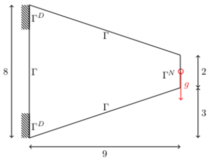
Figure 1: Scheme of a 2D cantilever beam clamped on $\Gamma^{D}$, with a load $g$ applied on the boundary $\Gamma^{N}$ and free boundaries $\Gamma$.

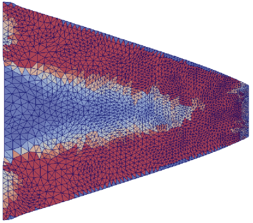
(a) Bulky structure.

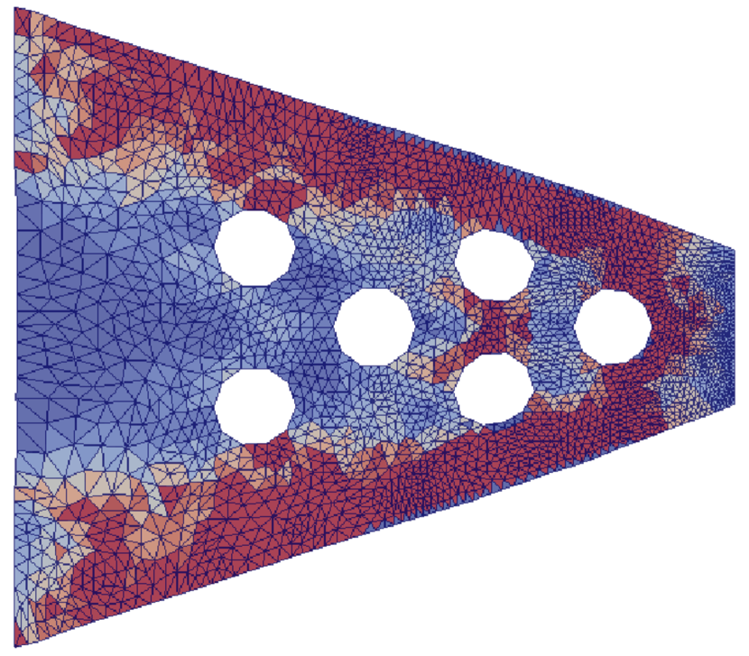
(b) Structure with six holes.

Figure 2: Initial shape and computational mesh for (a) a bulky cantilever and (b) a structure featuring six holes. Density distribution of the elastic energy within the range (a) $(0,1.5\cdot 10^{-3})$ and (b) $(0,3\cdot 10^{-3})$, the lower values being in blue and the higher ones in red.

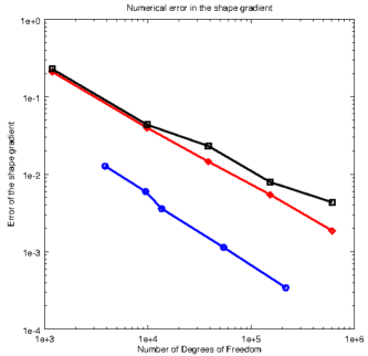
Figure 3: Experimental convergence rate of the error in the shape gradient computed using the surface expression based on the pure displacement formulation (black squares), the corresponding volumetric expression (red diamond) and the dual mixed formulation (blue circle) with respect to the number of Degrees of Freedom.

6.1 Experimental analysis of the convergence of the error in the shape gradient

In order to establish an experimental convergence rate for the discretization error associated with the approximation of the pure displacement and the dual mixed formulations of the linear elasticity problem, we consider the cantilever beam described in figure 1. In particular, we consider the domain featuring six holes depicted in figure 2b. Owing to the fact that the analytical solution of the linear elasticity problem on the aforementioned domain $\Omega$ is not known, we solve the linear elasticity problem on an extremely fine mesh and we consider the resulting solution as the exact solution of the problem under analysis. The discretization of the pure displacement formulation of the state problem is performed using $\mathbb{P}^{1}\times\mathbb{P}^{1}$ Finite Element functions to approximate the displacement field. For the dual mixed formulation, we consider the scheme described in subsection 2.3 and we approximate the stress tensor using $BDM_{1}\times BDM_{1}$ Finite Elements, the displacement field via $\mathbb{P}^{0}\times\mathbb{P}^{0}$ and the Lagrange multiplier by means of a $\mathbb{P}^{0}$ function.
In figure 3, we present the convergence history of the discretization error in the shape gradient with respect to the number of Degrees of Freedom using the surface expression based on the pure displacement formulation and the volumetric expressions previously derived. In particular, we observe that under uniform mesh refinements the surface expression based on the pure displacement formulation is less accurate and presents a slower convergence rate than the corresponding volumetric one. Moreover, using the dual mixed formulation the numerical error in the shape gradient is furtherly lowered and the blue curve seems slightly steeper than the red one. Thus, from the numerical experiments it seems that the volumetric shape gradient obtained from the dual mixed formulation of the problem may provide better convergence rate than the corresponding expression based on the pure displacement formulation. Nevertheless, this conjecture remains to be proved and a rigorous analysis of the convergence rate by means of a priori estimates of the error in the shape gradient is necessary.

6.2 Boundary Variation Algorithm using the pure displacement and the dual mixed formulations

In this subsection, we apply the Boundary Variation Algorithm described in subsection 3.1 to minimize the compliance of the cantilever in figure 1 under a volume constraint. In particular, the volume of the structure under analysis is set to its initial value $V_{0}$ and we aim to construct an optimal shape that minimizes the compliance while preserving as much as possible the value $V_{0}$ of the volume. As discussed in section 3, the volume constraint is handled through a Lagrange multiplier $\gamma$. From a theoretical point of view, the value of the Lagrange multiplier should be updated at each iteration in order for the optimal shape to fulfill the volume constraint when the algorithm converges. Nevertheless, enforcing the volume constraint at each iteration would highly increase the complexity of the algorithm and consequently its computational cost. Thus we consider a constant Lagrange multiplier at each iteration of the strategy and starting from the previously computed value $\gamma$, we increase it if the current volume $V$ is greater than the target $V_{0}$ and we decrease it otherwise.

As extensively discussed in [34, 35, 33], a key aspect of shape optimization procedures is the choice of the criterion to stop the evolution of the optimization strategy. In order to compare the expressions (4.15) and (5.18) of the shape gradient of the compliance, we consider an a priori fixed number of iterations for the BVA under analysis. Moreover, the number of connected regions inside the domain is set at the beginning of the procedure and the deformation of the shape is performed via a moving mesh approach. In the rest of this subsection, we present two test cases for the optimal design of the cantilever in figure 1, that is a bulky structure (Fig. 2a) and a porous one featuring six internal holes (Fig. 2b). All the numerical simulations are obtained using FreeFem++ [38].

Bulky cantilever beam

We consider the initial configuration in figure 2a. The volume of the structure under analysis is $V_{0}=45$ and we set the initial value of the Lagrange multiplier to $\gamma_{0}=0.1$. In figure 4, we present the shapes obtained using the Boundary Variation Algorithm based on the expressions (4.15) and (5.18) of the shape gradient of the compliance. In particular, we remark that the variant of the BVA which exploits the shape gradient computed via the dual mixed variational formulation of the linear elasticity problem is able to construct configurations in which the total elastic energy is lower than in the corresponding cases obtained starting from the pure displacement formulation of the problem. This remark is confirmed by the comparison plots in figure 5 where the BVA based on the dual mixed formulation is depicted by blue curves whereas the red ones represent the results obtained starting from the pure displacement formulation. As a matter of fact, the former approach appears more robust than the latter one: the BVA based on the dual mixed formulation improves both the compliance and the functional $L(\Omega)$ during several iterations, whereas at the beginning of the evolution, the variant exploiting the pure displacement formulation reduces the compliance by enlarging the volume of the structure, thus deteriorating the corresponding value of $L(\Omega)$ (Fig. 5b). In a second phase, the BVA based on the pure displacement formulation is able to better control the variation of the volume and the final shapes obtained by the two algorithms have comparable sizes (Fig. 5c). Nevertheless, the overall improvement of the compliance is far more limited when using the pure displacement formulation with respect to the one observed starting from the dual mixed formulation (Fig. 5a).

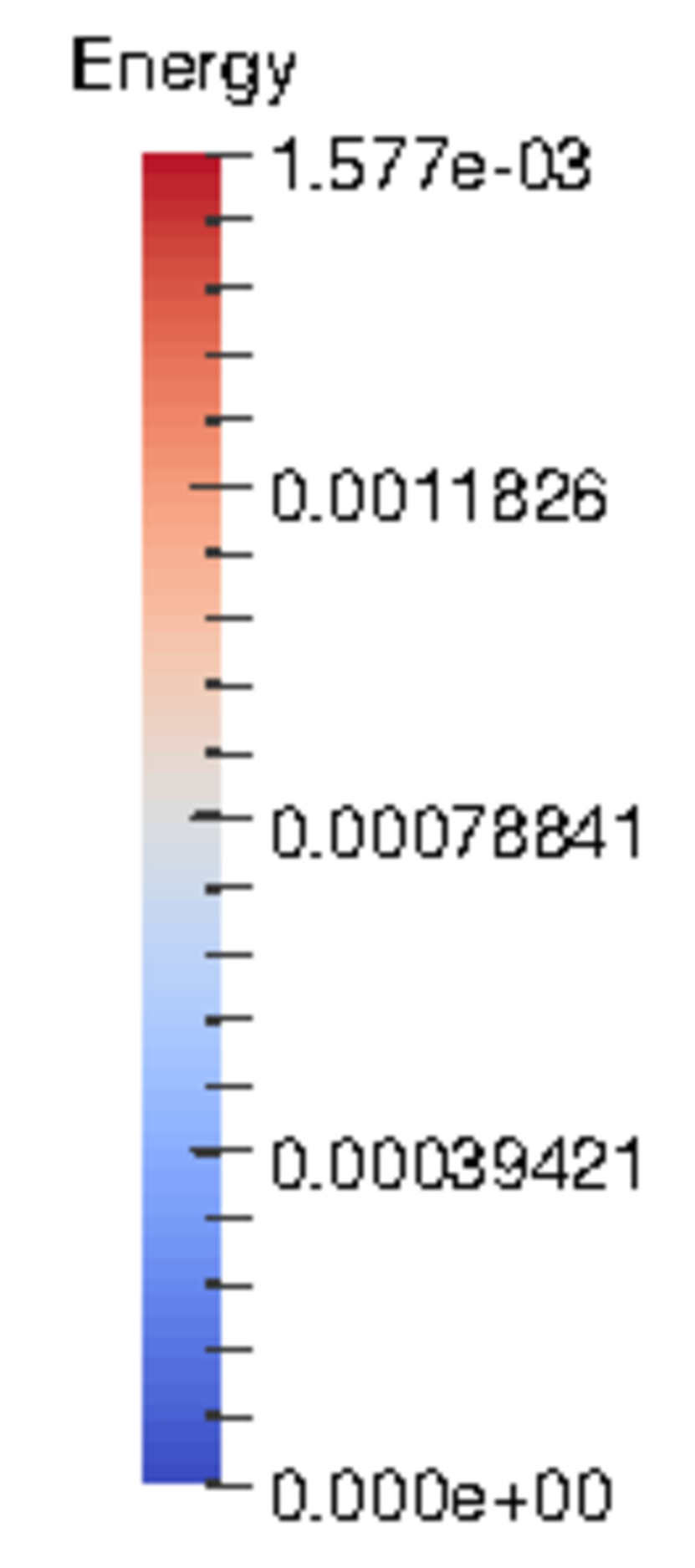
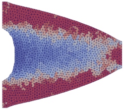
(a) 10 iterations.

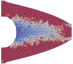
(b) 20 iterations.

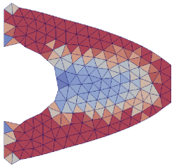
(c) 30 iterations.

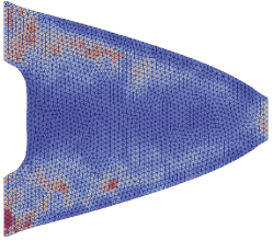
(d) 10 iterations.

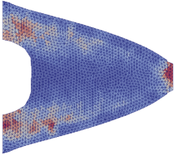
(e) 20 iterations.

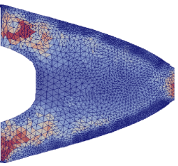
(f) 30 iterations.

Figure 4: Comparison of the BVA after 10, 20 and 30 iterations. At the top: BVA based on the expression of the shape gradient computed using the pure displacement formulation of the linear elasticity problem. At the bottom: BVA using the shape gradient arising from the dual mixed variational formulation. Density distribution of the elastic energy within the range $(0,1.5\cdot 10^{-3})$, the lower values being in blue and the higher ones in red.

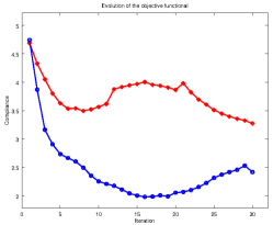
(a) Compliance $J(\Omega)$.

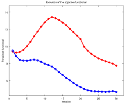
(b) Penalized functional $L(\Omega)$.

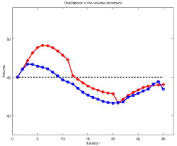
(c) Volume $V(\Omega)$.

Figure 5: Evolution of the (a) compliance $J(\Omega)$, (b) penalized functional $L(\Omega)=J(\Omega)+\gamma V(\Omega)$ and (c) volume $V(\Omega)$ using the BVA. Results obtained using the pure displacement formulation (red diamond) and the dual mixed one (blue circle). The reference volume $V_{0}$ is represented by a black dashed line in (c).

Cantilever beam with six holes

The initial shape for the cantilever beam with six holes is depicted in figure 2b and features a reference volume $V_{0}=40.59$ and an initial Lagrange multiplier equal to $\gamma_{0}=0.13$. As for the case of the bulky cantilever, we present snapshots of the shapes obtained at different iterations of the Boundary Variation Algorithm using both the pure displacement and the dual mixed formulation of the linear elasticity problem (Fig. 6). Moreover, a qualitative analysis of the evolution of the compliance and of the variation of the volume is discussed starting from figure 7. As previously remarked, the Boundary Variation Algorithm based on the dual mixed formulation of the linear elasticity problem leads to configurations with lower elastic energy. Figures 7a and 7b confirm that the variant of the BVA using the dual mixed formulation generates a sequence of shapes that improve the objective functional for several subsequent iterations. On the contrary, the pure displacement formulation leads to a less robust strategy in which at the beginning of the optimization process, the compliance is reduced by increasing the volume of the structure. Concerning the BVA based on the dual mixed formulation, the comparison of figure 6e with figure 6f, highlights that only minor modifications of the shape are performed by the algorithm from iteration 20 to iteration 30. As a matter of fact, the evolution of the volume (Fig. 7c) shows that after having identified a configuration with low compliance the algorithm tends to correct the shape in order to fulfill the volume constraint which has been violated during the initial iterations. As highlighted by the test case of the bulky cantilever, the Boundary Variation Algorithm based on the dual mixed formulation is able to construct structures with lower compliance than the configurations generated using the pure displacement formulation (Fig. 7a). Nevertheless, both the final configuration in figure 6c and the one in figure 6f, present some issues. On the one hand, the pure displacement solution presents kinks responsible for low compliance near the regions $\Gamma^{D}$ where the structure is clamped. On the other hand, the shape obtained by the dual mixed formulation features thin components which may be critical to handle during the manufacturing process. Both these issues may be potentially influenced by the choice of explicitly representing the geometry through the computational mesh and the consequent moving mesh approach to deform the domain. In order to bypass these issues, an implicit description of the geometry may be employed.

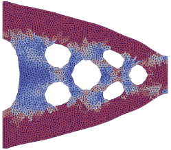
(a) 10 iterations.

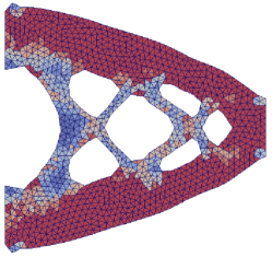
(b) 20 iterations.

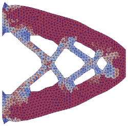
(c) 30 iterations.

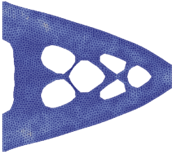
(d) 10 iterations.

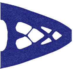
(e) 20 iterations.

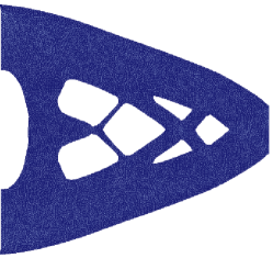
(f) 30 iterations.

Figure 6: Comparison of the BVA after 10, 20 and 30 iterations. At the top: BVA based on the expression of the shape gradient computed using the pure displacement formulation of the linear elasticity problem. At the bottom: BVA using the shape gradient arising from the dual mixed variational formulation. Density distribution of the elastic energy within the range $(0,3\cdot 10^{-3})$, the lower values being in blue and the higher ones in red.

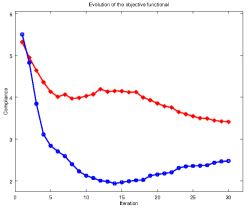
(a) Compliance $J(\Omega)$.

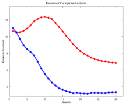
(b) Penalized functional $L(\Omega)$.

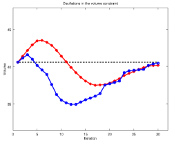
(c) Volume $V(\Omega)$.

Figure 7: Evolution of the (a) compliance $J(\Omega)$, (b) penalized functional $L(\Omega)=J(\Omega)+\gamma V(\Omega)$ and (c) volume $V(\Omega)$ using the BVA. Results obtained using the pure displacement formulation (red diamond) and the dual mixed one (blue circle). The reference volume $V_{0}$ is represented by a black dashed line in (c).

Concerning the computational cost of the overall optimization procedures, it is important to remark that the dual mixed formulation features more variables (stress tensor $\sigma_{\Omega}$, displacement field $u_{\Omega}$ and Lagrange multiplier $\eta_{\Omega}$) than the pure displacement one which - as the name states - solely relies on the displacement field $u_{\Omega}$. From a practical point of view, this results in a higher number of Degrees of Freedom in the discrete problem and consequently a higher computational cost. Moreover, by comparing the first and the second lines of figures 4 and 6, we remark that the computations of the BVA based on the dual mixed formulation were performed on finer meshes than the ones used for the pure displacement one. This turned out to be necessary in order to retrieve an accurate solution of the dual mixed Finite Element problem of linear elasticity, whereas the pure displacement formulation may be easily approximated using Lagrangian Finite Element functions as long as one avoids the nearly incompressible and the incompressible case. Eventually, the linear system obtained by the discretization discussed in subsection 2.3 may be extremely ill-posed and the construction of appropriate preconditioners (cf. e.g. [41]) may be necessary. Hence, though the preliminary numerical results suggest that the BVA based on the dual mixed formulation is the best choice when dealing with the minimization of the compliance in linear elasticity, the higher computational cost and the additional numerical difficulties of the overall strategy have to be taken into account to provide a global evaluation of the method. Within this context, additional investigations have to be performed both from a theoretical point of view (e.g. a priori estimate of the error in the shape gradient) and from a computational one, by optimizing and improving the resolution strategy outlined above.

7 Conclusion

To the best of our knowledge, the results in this article are the first attempt to derive volumetric expressions of the shape gradient of a shape-dependent functional within the framework of linear elasticity. In particular, we computed two novel expressions of the shape gradient of the compliance starting from the pure displacement and the dual mixed formulations of the governing equation. A preliminary comparison of the aforementioned expressions by means of numerical simulations showed extremely promising results, especially using the dual mixed variational formulation of the linear elasticity equation. As a matter of fact, the global optimization strategy based on this approach seems more robust than the one obtained from the pure displacement formulation and is able to further reduce the compliance of the structure under analysis. Nevertheless, a rigorous and detailed analysis both from an analytical and a numerical point of view is necessary to validate the aforementioned statement. Concerning the analytical derivation of the volumetric shape gradient of the compliance, a rigorous proof of the equivalence of the expressions obtained using the pure displacement and the dual mixed variational formulations of the linear elasticity problem is required. Moreover, following the analysis performed for the elliptic case in [39], a priori estimates of the error in the shape gradient may be derived. This analysis seems particularly interesting since it may provide additional information on the convergence of the shape gradient using different discretization techniques, thus possibly fostering one formulation over the other to achieve better accuracy in the approximation of the shape gradient.

It. $j$	$L(\Omega_{j})$	$\langle d_{h}L(\Omega_{j}),\theta_{j}^{h}\rangle$	$L(\Omega_{j+1})$
1	$9.38$	$-5.7\cdot 10^{-1}$	$9.25$
5	$9.99$	$-6.61\cdot 10^{-2}$	$10.52$
10	$12.80$	$-1.05\cdot 10^{-1}$	$13.19$
15	$12.78$	$-9.4\cdot 10^{-2}$	$12.46$
25	$8.58$	$-3.61\cdot 10^{-2}$	$8.4$
30	$7.54$	$-9.52\cdot 10^{-3}$	$-$

(a) Test in fig. 5 - Pure displacement formulation.

It. $j$	$L(\Omega_{j})$	$\langle d_{h}L(\Omega_{j}),\theta_{j}^{h}\rangle$	$L(\Omega_{j+1})$
1	$9.49$	$-4.78$	$8.83$
6	$8.37$	$-7.28\cdot 10^{-1}$	$8.43$
10	$7.95$	$-7.88\cdot 10^{-1}$	$7.79$
15	$6.62$	$-5.55\cdot 10^{-1}$	$6.3$
28	$4.68$	$-6.55\cdot 10^{-1}$	$4.74$
30	$4.66$	$-6.21\cdot 10^{-1}$	$-$

(b) Test in fig. 5 - Dual mixed formulation.

It. $j$	$L(\Omega_{j})$	$\langle d_{h}L(\Omega_{j}),\theta_{j}^{h}\rangle$	$L(\Omega_{j+1})$
1	$10.64$	$-1.00$	$10.48$
3	$10.50$	$-3.68\cdot 10^{-1}$	$10.66$
9	$12.30$	$-1.74\cdot 10^{-1}$	$12.34$
15	$10.61$	$-1.04\cdot 10^{-1}$	$10.06$
25	$7.16$	$-1.1\cdot 10^{-2}$	$7.05$
30	$6.82$	$-2.75\cdot 10^{-3}$	$-$

(c) Test in fig. 7 - Pure displacement formulation.

It. $j$	$L(\Omega_{j})$	$\langle d_{h}L(\Omega_{j}),\theta_{j}^{h}\rangle$	$L(\Omega_{j+1})$
1	$11.01$	$-15.32$	$10.48$
5	$8.49$	$-2.55$	$8.12$
10	$5.50$	$-1.29$	$4.95$
18	$3.18$	$-1.36$	$3.19$
28	$3.32$	$-2.06$	$3.36$
30	$3.37$	$-2.18$	$-$

(d) Test in fig. 7 - Dual mixed formulation.

Table 1: Boundary Variation Algorithm based on the pure displacement formulation (left) and on the dual mixed formulation (right) of the linear elasticity problem. On the first line: test case in figure 5. On the second line: test case in figure 7. Evolution of the penalized objective functional $L(\Omega)$ with respect to the iteration number. In yellow: the cases in which the discretized direction $\theta^{h}$ fails to be a genuine descent direction for $L(\Omega)$ despite being $\langle d_{h}L(\Omega),\theta^{h}\rangle<0$.

The numerical results in section 6 highlight some issues associated with the application of the Boundary Variation Algorithm to the minimization of the compliance in structural optimization. On the one hand, it is straightforward to observe (Fig. 5 and 7) that the direction computed using the discretized shape gradient is not always a genuine descent direction for the functional under analysis. To remedy this issue, in [34, 35, 33] we proposed a variant of the BVA - named Certified Descent Algorithm (CDA) - that couples a gradient-based optimization strategy with a posteriori estimators of the error in the shape gradient. This remark is confirmed by table 1 in which we observe that despite being $\langle d_{h}L(\Omega),\theta^{h}\rangle<0$, the functional $L(\Omega)$ may increase when the shape is perturbed accordingly to the field $\theta^{h}$. Ongoing investigations focus on the application of the aforementioned CDA to the minimization of the compliance discussed in this article. On the other hand, the choice of explicitly representing the geometry and deforming it by moving the computational mesh is responsible for the degradation of the final shapes computed by the algorithm. Currently, we are investigating the approach proposed by Allaire et al. in [3] that exploits an implicit description of the geometry via a level-set function and propagates it by solving an Hamilton-Jacobi equation.

Eventually mixed formulations of the linear elasticity problem with strongly-enforced symmetry of the stress tensor may be investigated, e.g. the Hellinger-Reissner formulation approximated by means of Arnold-Winther Finite Element spaces (cf. [16, 10]) and the Tangential-Displacement Normal-Normal-Stress (TD-NNS) formulation recently proposed by Pechstein and Schöberl in [45].

Acknowledgements

Part of this work was developed during a stay of the first author at the Laboratoire J.A. Dieudonné at Université de Nice-Sophia Antipolis whose support is warmly acknowledged.

References

• [1] S. Adams and B. Cockburn. A mixed finite element method for elasticity in three dimensions. J. Sci. Comput., 25(3):515–521, 2005.
• [2] G. Allaire. Conception optimale de structures. Springer, 2006.
• [3] G. Allaire, C. Dapogny, and P. Frey. Shape optimization with a level set based mesh evolution method. Comput. Method. Appl. M., 282:22 – 53, 2014.
• [4] G. Allaire, F. Jouve, and G. Michailidis. Molding direction constraints in structural optimization via a level-set method. working paper or preprint, Dec. 2015.
• [5] G. Allaire, F. Jouve, and G. Michailidis. Thickness control in structural optimization via a level set method. Struct. Multidiscip. O., 53(6):1349–1382, 2016.
• [6] G. Allaire and O. Pantz. Structural optimization with FreeFem++. Struct. Multidiscip. O., 32(3):173–181, 2006.
• [7] M. Alnæs, J. Blechta, J. Hake, A. Johansson, B. Kehlet, A. Logg, C. Richardson, J. Ring, M. Rognes, and G. Wells. The FEniCS Project Version 1.5. Archive of Numerical Software, 3(100), 2015.
• [8] M. Amara and J. M. Thomas. Equilibrium finite elements for the linear elastic problem. Numer. Math., 33(4):367–383, 1979.
• [9] D. N. Arnold. Mixed finite element methods for elliptic problems. Comput. Method. Appl. M., 82(1-3):281–300, 1990. Reliability in computational mechanics (Austin, TX, 1989).
• [10] D. N. Arnold, G. Awanou, and R. Winther. Finite elements for symmetric tensors in three dimensions. Math. Comput., 77(263):1229–1251, 2008.
• [11] D. N. Arnold, F. Brezzi, and J. Douglas, Jr. PEERS: a new mixed finite element for plane elasticity. Japan J. Appl. Math., 1(2):347–367, 1984.
• [12] D. N. Arnold, J. Douglas, and C. P. Gupta. A family of higher order mixed finite element methods for plane elasticity. Numer. Math., 45(1):1–22, 1984.
• [13] D. N. Arnold and R. S. Falk. A new mixed formulation for elasticity. Numer. Math., 53(1-2):13–30, 1988.
• [14] D. N. Arnold, R. S. Falk, and R. Winther. Differential complexes and stability of finite element methods. II. The elasticity complex. In Compatible spatial discretizations, volume 142 of IMA Vol. Math. Appl., pages 47–67. Springer, New York, 2006.
• [15] D. N. Arnold, R. S. Falk, and R. Winther. Mixed finite element methods for linear elasticity with weakly imposed symmetry. Math. Comput., 76(260):1699–1723, 2007.
• [16] D. N. Arnold and R. Winther. Mixed finite elements for elasticity. Numer. Math., 92(3):401–419, 2002.
• [17] M. Berggren. A unified discrete–continuous sensitivity analysis method for shape optimization. In W. Fitzgibbon, Y. Kuznetsov, P. Neittaanmäki, J. Périaux, and O. Pironneau, editors, Applied and Numerical Partial Differential Equations: Scientific Computing in Simulation, Optimization and Control in a Multidisciplinary Context, pages 25–39. Springer Netherlands, Dordrecht, 2010.
• [18] D. Boffi, F. Brezzi, and M. Fortin. Reduced symmetry elements in linear elasticity. Commun. Pure Appl. Anal., 8(1):95–121, 2009.
• [19] D. Boffi, F. Brezzi, and M. Fortin. Mixed finite element methods and applications, volume 44 of Springer Series in Computational Mathematics. Springer, Heidelberg, 2013.
• [20] D. Braess. Finite Elements: Theory, Fast Solvers, and Applications in Solid Mechanics. Cambridge University Press, 2001.
• [21] S. C. Brenner and L. R. Scott. The mathematical theory of finite element methods, volume 15 of Texts in Applied Mathematics. Springer, New York, third edition, 2008.
• [22] F. Brezzi. On the existence, uniqueness and approximation of saddle-point problems arising from lagrangian multipliers. ESAIM: Math. Model. Num., 8(R2):129–151, 1974.
• [23] F. Brezzi, J. Douglas, Jr., and L. D. Marini. Recent results on mixed finite element methods for second order elliptic problems. In Vistas in applied mathematics, Transl. Ser. Math. Engrg., pages 25–43. Optimization Software, New York, 1986.
• [24] C. Carstensen, M. Eigel, and J. Gedicke. Computational competition of symmetric mixed FEM in linear elasticity. Comput. Method. Appl. M., 200(41–44):2903 – 2915, 2011.
• [25] C. Carstensen, D. Günther, J. Reininghaus, and J. Thiele. The Arnold-Winther mixed FEM in linear elasticity. part I: Implementation and numerical verification. Comput. Method. Appl. M., 197(33–40):3014 – 3023, 2008.
• [26] P. G. Ciarlet. Mathematical elasticity. Vol. I, volume 20 of Studies in Mathematics and its Applications. North-Holland Publishing Co., Amsterdam, 1988. Three-dimensional elasticity.
• [27] R. Correa and A. Seeger. Directional derivative of a minimax function. Nonlinear Anal.-Theor., 9(1):13–22, 1985.
• [28] M. Delfour and J.-P. Zolésio. Shapes and geometries: analysis, differential calculus, and optimization. SIAM, Philadelphia, USA, 2001.
• [29] P. Duysinx, L. Van Miegroet, E. Lemaire, O. Brüls, and M. Bruyneel. Topology and generalized shape optimization: Why stress constraints are so important? Int. J. Simul. Multidisci. Des. Optim., 2(4):253–258, 2008.
• [30] M. Farhloul and M. Fortin. Dual hybrid methods for the elasticity and the Stokes problems: a unified approach. Numer. Math., 76(4):419–440, 1997.
• [31] B. Fraeijs de Veubeke. Stress function approach. In Proceedings of the World Congress on Finite Element Methods in Structural Mechanics, volume 1. Dorset, 1975.
• [32] Z. Gao, Y. Ma, and H. Zhuang. Optimal shape design for Stokes flow via minimax differentiability. Math. Comput. Model., 48(3-4):429–446, 2008.
• [33] M. Giacomini. An equilibrated fluxes approach to the Certified Descent Algorithm for shape optimization using conforming Finite Element and Discontinuous Galerkin discretizations. Submitted, 2016.
• [34] M. Giacomini, O. Pantz, and K. Trabelsi. An a posteriori error estimator for shape optimization: application to EIT. J. Phys.: Conf. Ser., 657(1):012004, 2015.
• [35] M. Giacomini, O. Pantz, and K. Trabelsi. Certified Descent Algorithm for shape optimization driven by fully-computable a posteriori error estimators. ESAIM: Contr. Op. Ca. Va., 2016. To appear.
• [36] P. Gould. Introduction to Linear Elasticity. Introduction to Linear Elasticity. Springer, 1993.
• [37] J. Hadamard. Mémoire sur le problème d’analyse relatif à l’équilibre des plaques élastiques encastrées. B. Soc. Math. Fr., 1907.
• [38] F. Hecht. New development in FreeFem++. J. Numer. Math., 20(3-4):251–265, 2012.
• [39] R. Hiptmair, A. Paganini, and S. Sargheini. Comparison of approximate shape gradients. BIT, 55(2):459–485, 2015.
• [40] C. O. Horgan. Korn’s inequalities and their applications in continuum mechanics. SIAM Rev., 37(4):491–511, 1995.
• [41] A. Klawonn and G. Starke. A preconditioner for the equations of linear elasticity discretized by the peers element. Numer. Linear Algebr., 11(5-6):493–510, 2004.
• [42] J. E. Marsden and T. J. R. Hughes. Mathematical foundations of elasticity. Dover Publications, Inc., New York, 1994. Corrected reprint of the 1983 original.
• [43] M. E. Morley. A family of mixed finite elements for linear elasticity. Numer. Math., 55(6):633–666, 1989.
• [44] J. Nocedal and S. Wright. Numerical optimization. Springer-Verlag New York, USA, 1999.
• [45] A. Pechstein and J. Schöberl. Tangential-displacement and normal-normal-stress continuous mixed finite elements for elasticity. Math. Mod. Meth. Appl. S., 21(8):1761–1782, 2011.
• [46] P.-A. Raviart and J. M. Thomas. A mixed finite element method for 2nd order elliptic problems. In Mathematical aspects of finite element methods (Proc. Conf., Consiglio Naz. delle Ricerche (C.N.R.), Rome, 1975), pages 292–315. Lecture Notes in Math., Vol. 606. Springer, Berlin, 1977.
• [47] E. Reissner. On a variational theorem in elasticity. J. Math. Phys. Camb., 29(1-4):90–95, 4 1950.
• [48] M. E. Rognes, R. C. Kirby, and A. Logg. Efficient assembly of $H({\rm div})$ and $H({\rm curl})$ conforming finite elements. SIAM J. Sci. Comput., 31(6):4130–4151, 2009/10.
• [49] E. Stein and R. Rolfes. Mechanical conditions for stability and optimal convergence of mixed finite elements for linear plane elasticity. Comput. Method. Appl. M., 84(1):77–95, 1990.
• [50] R. Stenberg. On the construction of optimal mixed finite element methods for the linear elasticity problem. Numer. Math., 48(4):447–462, 1986.
• [51] R. Stenberg. A family of mixed finite elements for the elasticity problem. Numer. Math., 53(5):513–538, 1988.
• [52] R. Stenberg. Two low-order mixed methods for the elasticity problem. In The mathematics of finite elements and applications, VI (Uxbridge, 1987), pages 271–280. Academic Press, London, 1988.
• [53] K. Svanberg. The method of moving asymptotes—a new method for structural optimization. Int. J. Numer. Meth. Eng., 24(2):359–373, 1987.
• [54] J.-M. Thomas. Méthode des éléments finis hybrides duaux pour les problémes elliptiques du second ordre. ESAIM: Math. Model. Num., 10(R3):51–79, 1976.
• [55] G. N. Vanderplaats and F. Moses. Structural optimization by methods of feasible directions. Comput. Struct., 3(4):739 – 755, 1973.