Dynamics of Dirac solitons in networks

Abstract

We study dynamics of Dirac solitons in prototypical networks modeling them by the nonlinear Dirac equation on metric graphs. Stationary soliton solutions of the nonlinear Dirac equation on simple metric graphs are obtained. It is shown that these solutions provide reflectionless vertex transmission of the Dirac solitons under suitable conditions. The constraints for bond nonlinearity coefficients, conjectured to represent necessary conditions for allowing reflectionless transmission over a Y-junction are derived. The Y-junction considerations are also generalized to a tree network. The analytical results are confirmed by direct numerical simulations.

1 Introduction

Nonlinear evolution equations on networks have attracted much attention recently [1, 2, 3, 4, 5, 6, 7, 8, 9, 10]. Such interest is caused by a broad variety of potential applications of the nonlinear wave dynamics and soliton transport in networks, such as Bose-Einstein condensates (BECs) in branched traps, Josephson junction networks, the DNA double helix, polymer chains, etc.

Despite the rapidly growing interest in wave dynamics on networks, most of the studies are mainly focused on nonrelativistic wave equations such as the nonlinear Schrödinger (NLS) equation [1, 2, 3, 4, 5, 6, 7, 10]. Nevertheless, there is a number of works on the sine-Gordon (sG) equation in branched systems [8, 9, 11]. However, relativistic wave equations such as the nonlinear Klein-Gordon and Dirac equations are important in field theory and condensed matter physics and hence exploring them on metric graphs is of interest in its own right. These graphs consist of a system of bonds which are connected at one or more vertices (branching points). The connection rule is associated with the topology of a graph. When the bonds can be assigned a length, the graph is called a metric graph.

In this paper we address the problem of the nonlinear Dirac equation on simple metric graphs by focusing on conservation laws and soliton transmission at the graph vertices. Our prototypical example will be the Y-junction. Early studies of the nonlinear Dirac equation date back to Thirring [12] and Gross-Neveu [13] models of field theory. Integrability, the nonrelativistic limit and exact solutions of the relevant models have been considered in, e.g., [14, 15, 16, 17, 18] among others. A potential application of the nonlinear Dirac equation to neutrino oscillations was discussed in [19]. Recently, the possibility of experimental realization of Dirac solitons in Bose-Einstein condensates in honeycomb optical lattices was discussed in [21] where the nonlinear Dirac equation was derived. Further analysis of this setting in Refs. [22, 23, 24, 26] has excited a rapidly growing interest in the nonlinear Dirac equation and its soliton solutions (see, e.g. [27]-[49]). In [27, 28, 31, 32, 33, 34], a detailed study of soliton solutions for different types of nonlinearity, their stability and discussions of conservation laws were presented. These developments have, in turn, had an impact also on the mathematical literature where the stability of solutions for different forms of the nonlinear Dirac equation was explored in [29, 30, 36]. In [37]-[41], the stability of Gross-Neveu solitons in both 1d and 3d and for other nonlinear Dirac models an important energy-based stability criterion was developed. The numerical corroboration of the stability for solitary waves and vortices in 2D nonlinear Dirac models of the Gross-Neveu type was considered quite recently in [35].

Dirac solitons in branched systems can, in principle, be experimentally realized in different systems of optics, but also envisioned elsewhere (e.g. in atomic physics etc.).

A relevant such possibility consists of the discrete waveguide arrays of [44, 49] that can be formulated as a branched system to be described (in the appropriate long wavelength limit [44]) by a nonlinear Dirac equation on metric graphs. Such networks in optical systems have been proposed, e.g., earlier in [50]. More exotic possibilities can be envisioned in branched networks of honeycomb (i.e., armchair nanoribbon) optical lattices for atomic BECs [23], although we will not focus on the latter here.

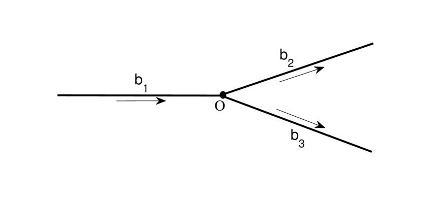
Figure 1: Metric star graph

In the present work, we focus on a prototypical example of exact solutions and transport of Dirac solitons through the network vertices. In particular, we show that under certain constraints, exact soliton solutions of the nonlinear Dirac equation on simple metric graphs can be obtained. The identified soliton solutions provide reflectionless transmission of the Dirac solitons at the vertices. This renders possible the tuning of the transport properties of a network in such a way that it can provide ballistic transport of the Dirac solitons. This paper is organized as follows: In the next section we give the formulation of the problem on a metric star graph which includes the derivation of the vertex boundary conditions. Section III presents soliton solutions of the nonlinear Dirac equation on a metric star graph for fixed and moving frames. Also, an analysis of the vertex transmission of the Dirac solitons on the basis of the numerical solution of the nonlinear Dirac equation is presented. In section IV we extend the treatment to a metric tree graph and discuss the extension to other simple topologies. Finally, section V presents some concluding remarks and a number of important directions for future work. These include a conjecture about the sufficient, yet not necessary nature of our vertex conditions towards ensuring reflectionless transmission.

2 Conservation laws and vertex boundary conditions

The nonlinear Dirac system that we are going to explore, i.e., specifically the Gross-Neveu model, follows from the Lagrangian (in the units $\hbar=c=1$) [27, 28, 31]

$$L=\frac{i}{2}\bar{\Psi}\gamma^{\mu}\partial_{\mu}\Psi-m\bar{\Psi}\Psi+\frac{g^{2}}{2}\left(\bar{\Psi}\Psi\right)^{2},\;\;\;\mu=0,1,$$ (1)

and describes interacting Dirac fields with $0$ and $1$ corresponding to time and coordinate variables, respectively. Here $g$ is the nonlinearity coefficient characterizing the strength of the nonlinear interaction. The field equations for this Lagrangian lead to the nonlinear Dirac model of the form

$$\left(i\gamma^{\mu}\partial_{\mu}-m\right)\Psi+g^{2}\left(\bar{\Psi}\Psi\right)\Psi=0,$$ (2)

where

$$\Psi(x,t)=\left(\begin{array}[]{cc}\phi(x,t)\\ \chi(x,t)\end{array}\right);\;\;\ \bar{\Psi}=\Psi^{\dagger}\gamma^{0}=(\phi^{*}(x,t),-\chi^{*}(x,t)),$$ (3)

and $\gamma^{0}=\left(\begin{array}[]{cc}1&0\\ 0&-1\end{array}\right),\,\gamma^{1}=\left(\begin{array}[]{cc}0&1\\ -1&0\end{array}\right)$.

For a metric star graph consisting of three semi-infinite bonds (see, e.g., Fig. 1), the Lagrangian density of the nonlinear Dirac field for each bond can be written as $L_{j}$ where $j$ parametrizes the bond and $L$ for each is of the form of Eq. (1).

The field equation following from this Lagrangian density can be written as Eq. (2) before, where the spatial coordinates are defined as $x_{1}\in(-\infty,0]$ and $x_{2,3}\in[0,\infty)$, while 0 coincides with the graph vertex.

The formulation of an evolution set of equations on metric graphs requires imposing vertex boundary conditions which provide “gluing” of the graph bonds at the graph vertices. For the linear Dirac equation on a metric graph studied earlier by Bolte and Harrison in [51], the general vertex boundary conditions have been derived from the self-adjointness of the Dirac operator on a graph. In that case such conditions led to Kirchhoff rules and continuity of the wave function at the graph vertex [51]. However, for the nonlinear problem in order to derive vertex BCs, it is arguably more natural to use suitable conservation laws of the nonlinear flow, which give rise to appropriate BCs. For the nonlinear Dirac system fundamental conservation laws can be presented in terms of the momentum-energy tensor given by [27, 28]

$$T^{j}_{\mu\nu}=\frac{i}{2}[\bar{\Psi}_{j}\gamma^{\mu}\partial^{\nu}\Psi_{j}-\partial^{\nu}\bar{\Psi}_{j}\gamma^{\mu}\Psi_{j}]-g^{\mu\nu}L_{j},$$

where $g^{\mu\nu}=\left({\begin{array}[]{cc}1&0\\ 0&1\end{array}}\right)$.

The energy on each bond of a star graph can be written as

$$E_{j}=-\int_{b_{j}}T^{j}_{00}dx=-\int_{b_{j}}[\frac{i}{2}[\bar{\Psi}_{j}\gamma^{1}\partial_{x}\Psi_{j}\\ -\partial_{x}\bar{\Psi}_{j}\gamma^{1}\Psi_{j}]-m\bar{\Psi}_{j}\Psi_{j}+\frac{g_{j}^{2}}{2}(\bar{\Psi}_{j}\Psi_{j})^{2}]dx,$$

where integration is performed along the bond $b_{j}$. Here, to derive the vertex boundary conditions (VBC) we use conservations of charge and energy. The total charge for the star graph is defined as

$$Q=Q_{1}+Q_{2}+Q_{3},$$

where the charge for each bond is given by

$$Q_{j}=\int_{b_{j}}\left(|\phi_{j}|^{2}+|\chi_{j}|^{2}\right)dx.$$ (4)

The conservation of charge (Kirchhoff rule for charge current), $\dot{Q}=0$ yields the following vertex boundary condition:

$$\left.{\rm Re}\left[\phi_{1}\chi_{1}^{*}\right]\right|_{x=0}=\left.{\rm Re}\left[\phi_{2}\chi_{2}^{*}\right]\right|_{x=0}+\left.{\rm Re}\left[\phi_{3}\chi_{3}^{*}\right]\right|_{x=0}.$$ (5)

Here we used the asymptotic conditions

$$\Psi_{1}\to 0\;{\rm at}\;x\to-\infty\;{\rm and}\;\Psi_{2,3}\to 0\;{\rm at}\;x\to\infty.$$ (6)

We note that the boundary conditions (5) can be derived also from the conservation of the current density given by $j=\varphi\chi^{*}+\chi\varphi^{*}$.

The energy conservation, $\dot{E}=0$ leads to

$$\left.{\rm Im}\left[\phi_{1}\partial_{t}\chi_{1}^{*}+\chi_{1}\partial_{t}\phi_{1}^{*}\right]\right|_{x=0}$$

$$=\left.{\rm Im}\left[\phi_{2}\partial_{t}\chi_{2}^{*}+\chi_{2}\partial_{t}\phi_{2}^{*}\right]\right|_{x=0}+\left.{\rm Im}\left[\phi_{3}\partial_{t}\chi_{3}^{*}+\chi_{3}\partial_{t}\phi_{3}^{*}\right]\right|_{x=0}.$$

(7)

As per the above analysis, the VBC for NLDE on metric graphs have been obtained from the energy and charge conservation. However, the VBC given by Eqs. (5) can be fulfilled, if the following linear relations at the vertices are imposed (see Appendix for details):

$$\alpha_{1}\phi_{1}|_{x=0}=\alpha_{2}\phi_{2}|_{x=0}+\alpha_{3}\phi_{3}|_{x=0},$$

$$\frac{1}{\alpha_{1}}\chi_{1}|_{x=0}=\frac{1}{\alpha_{2}}\chi_{2}|_{x=0}=\frac{1}{\alpha_{3}}\chi_{3}|_{x=0},$$ (8)

where $\alpha_{1},\alpha_{2},\alpha_{3}$ are the real constants which will be determined below. In the following we will use Eqs. (8) as the vertex boundary conditions for Eq. (2) on a metric star graph. When applied to the exact soliton solutions of the NLDE, the VBC will lead to algebraic conditions connecting $\alpha_{j}$ and $g_{j}$, as will be derived in the next section. We note that in the linear limit ($g_{j}\to 0$) the vertex boundary conditions given by Eq. (8) preserve the self-adjointness of the (linear) Dirac equation on metric graph, i.e. belong to the class of general boundary conditions derived by Bolte and Harrison in [51].

3 Soliton dynamics and vertex transmission

In [27, 28, 31] the soliton solutions of the nonlinear Dirac equation on the line have been obtained in the form of standing wave solutions asymptoting to zero as $x\to\pm\infty$. Here, we use the same definition for soliton solutions of the nonlinear Dirac equation on the metric star graph presented in Fig. 1. We note in passing that for soliton solutions of the NLDE derived in the Refs.[27, 28, 31] all elements of the energy-momentum tensor, except $T_{00}$ become zero, i.e., $T_{01}=T_{10}=T_{11}=0$.

We look for the soliton solution of NLDE on a metric star graph in the form

$$\Psi_{j}(x,t)=\left(\begin{array}[]{cc}\psi_{1j}(x,t)\\ \psi_{2j}(x,t)\end{array}\right)=e^{-i\omega t}\left(\begin{array}[]{cc}A_{j}(x)\\ iB_{j}(x)\end{array}\right).$$ (9)

Then, from Eqs. (2) and (9) we have

$$\frac{dA_{j}}{dx}+(m+\omega)B_{j}-g_{j}^{2}(A_{j}^{2}-B_{j}^{2})B_{j}=0,$$ (10)

$$\frac{dB_{j}}{dx}+(m-\omega)A_{j}-g_{j}^{2}(A_{j}^{2}-B_{j}^{2})A_{j}=0.$$ (11)

The vertex boundary conditions for the functions $A_{j}$ and $B_{j}$ can be written as

$$\alpha_{1}A_{1}|_{x=0}=\alpha_{2}A_{2}|_{x=0}+\alpha_{3}A_{3}|_{x=0},$$

$$\frac{1}{\alpha_{1}}B_{1}|_{x=0}=\frac{1}{\alpha_{2}}B_{2}|_{x=0}=\frac{1}{\alpha_{3}}B_{3}|_{x=0}.$$ (12)

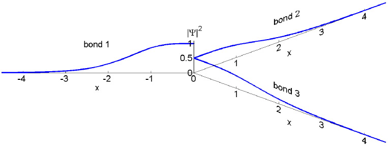
Figure 2: (Color online) Charge density, $|\Psi_{j}|^{2}=\Psi^{\dagger}\Psi=|A_{j}(x)|^{2}+|B_{j}(x)|^{2}$, plotted using the standing wave soliton solutions given by Eqs. (13) and (14)($x_{0}=0$) for $g_{1}=1,\;g_{2}=g_{3}=\sqrt{2}.$

A prototypical static solution of the system (10), (11) vanishing at $x\to\pm\infty$ can be written as [28]

$$A_{j}(x)=\sqrt{\frac{(m+\omega)\cosh^{2}(\beta(x-x_{0}))}{m+\omega\cosh(2\beta(x-x_{0}))}}\sqrt{\frac{2\beta^{2}}{g_{j}^{2}(m+\omega\cosh(2\beta(x-x_{0})))}},$$ (13)

$$B_{j}(x)=\sqrt{\frac{(m-\omega)\sinh^{2}(\beta(x-x_{0}))}{m+\omega\cosh(2\beta(x-x_{0}))}}\sqrt{\frac{2\beta^{2}}{g_{j}^{2}(m+\omega\cosh(2\beta(x-x_{0})))}},$$ (14)

where $x_{0}$ is the position of the soliton’s center of mass and $\beta=\sqrt{m^{2}-\omega^{2}}.$ In order for these solutions of Eqs. (10) and (11) to solve the problem on the metric graph, they need to also satisfy the vertex boundary conditions (12). This can be achieved if the constants $\alpha_{j}$ and coupling parameters $g_{j}$ fulfill the following conditions:

$$\frac{\alpha_{1}}{|g_{1}|}=\frac{\alpha_{2}}{|g_{2}|}+\frac{\alpha_{3}}{|g_{3}|}.$$ (15)

which stems from the first of Eqs. (8) and

$$\frac{\alpha_{2,3}}{\alpha_{1}}=\frac{|g_{1}|}{|g_{2,3}|},$$ (16)

in accordance with the second one of conditions (8). The combination of the two leads to the “sum rule”:

$$\frac{1}{g_{1}^{2}}=\frac{1}{g_{2}^{2}}+\frac{1}{g_{3}^{2}}.$$ (17)

It is important to note that this sum rule is derived by assuming that incoming wave comes from the first bond, $b_{1}$, while if it comes from the bond $b_{2}$ (or $b_{3}$) one should replace $g_{1}$ in Eq. (17) with $g_{2}$ (or $g_{3}$). In Fig. 2 plots of the soliton solutions of NLDE on metric star graph corresponding to Eqs. (13) and (14), satisfying the vertex conditions are given.

We note that soliton solutions given by Eqs.(13) and (14) describe the standing waves in metric graphs. The traveling wave (soliton) solutions of NLDE can be obtained by considering the case of the moving frame and taking into account the Lorentz invariance [28], in the case of the homogeneous domain (i.e., without a Y-junction). Assuming implicitly that the solitary wave is centered around a position well to the left of the origin, the Lorentz transformations between the frames moving with relative velocity, $v$ can be written as [28]

$$x^{\prime}=\gamma(x-vt);\;t^{\prime}=\gamma(t-vx),$$ (18)

where

$$\gamma=\frac{1}{\sqrt{1-v^{2}}}=\cosh\eta,\;\sinh\eta=\frac{v}{\sqrt{1-v^{2}}}.$$ (19)

Using these transformations, the traveling wave (soliton) solutions of the nonlinear Dirac equation in the moving frame determined by the constraints (15) can be written as

$$\psi_{1j}(x,t) = [\cosh(\eta/2)A_{j}(x^{\prime})+i\sinh(\eta/2)B_{j}(x^{\prime})]e^{-i\omega t^{\prime}},$$

$$\Psi_{2j}(x,t) = [\sinh(\eta/2)A_{j}(x^{\prime})+i\cosh(\eta/2)B_{j}(x^{\prime})]e^{-i\omega t^{\prime}}$$ (20)

where $x^{\prime},$ $t^{\prime}$ and $\eta$ are given by Eqs. (18) and (19).

It is important to note that this transformation does not affect the scaling dependence on the coupling parameters $g_{j}$. For that reason, we expect the form of Eqs. (15) to still be valid in the case of traveling/moving wave solutions.

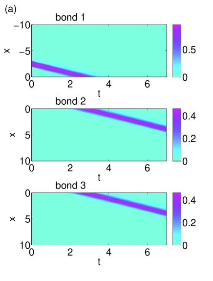
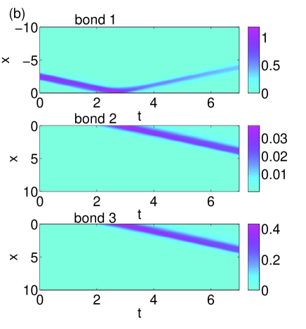
Figure 3: (Color online) Time and coordinate dependence of the charge density obtained from the numerical solution of Eq. (2) ($x_{0}=0$) for boundary conditions (8) for the case (a) when constraints (17) are fulfilled ($g_{1}=1,\;g_{2}=g_{3}=\sqrt{2}$), (b) when these constraints are not fulfilled ($g_{1}=1,\;g_{2}=\sqrt{2};g_{3}=3.5$).

To analyze the dynamics of the Dirac solitons on a metric graph, we solve numerically the time-dependent NLDE given by Eq. (2) for the vertex boundary conditions given by Eq. (8) by considering the an initially traveling waveform localized in bond 1, far from the vertex. We do this for the case when the constraint given by Eq. (17) is fulfilled, as well as for the case of arbitrary $g_{j}$ which do not respect the relevant constraints. Fig. 3(a) presents the plots of the solution of Eqs. (2) and (8) obtained numerically for the values of $g_{j}$ obeying the constraint (17). For vertex boundary conditions given by Eq.(12) parameters $\alpha_{j}$ are chosen as $\alpha_{2}=1/|g_{2}|$, $\alpha_{3}=1/|g_{3}|$, $\alpha_{1}=|g_{1}|(\alpha_{2}/|g_{2}|+\alpha_{3}/|g_{3}|)$. One can observe the absence of the vertex reflection in this case. Fig. 3(b) presents soliton solutions of nonlinear Dirac equation for the boundary conditions (8) obtained numerically for those values of $g_{j}$ which do not fulfill Eq. (17). Here, reflection can be clearly discerned. Fig. 4(a) shows the conservation of the energy and reflectionless transmission through the Y-junction during the propagation of Dirac soliton in graph. The emergence of the vertex reflection when the constraints (17) are not fulfilled, can also be seen from the Fig. 4(b). Here the vertex reflection coefficient, which is determined according to the definition $R=E_{1}(t=7)/E(t=7)$ (with $E(t=7)=E_{1}(t=7)+E_{2}(t=7)+E_{3}(t=7)$) is plotted as a function of $g_{3}$ for fixed values of $g_{1}$ and $g_{2}$. This systematic analysis clearly illustrates the necessity of the symmetric scenario of $g_{3}=\sqrt{2}$, consonant with our vertex sum rule, for reflection to be absent. A similar phenomenon was observed in the case of other nonlinear PDEs on metric graphs, such as the NLS and sG equations, considered earlier in the Refs.[1] and [11], respectively. For the initial condition corresponding to a traveling wave of the NLDE in the form of (20) centered at $x_{0}$, with initial velocity $v>0$ for $t\to+\infty$, our numerical computations provide strong evidence to the following fact. The solution can be asymptotically represented as a superposition of solitary waves in the branches associated with the second and third bonds, only if the condition (8) holds. In other words, under the necessary constraints (17), Eqs. (8) asymptotically lead to refectionless transmission through the vertex.

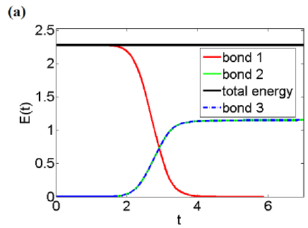
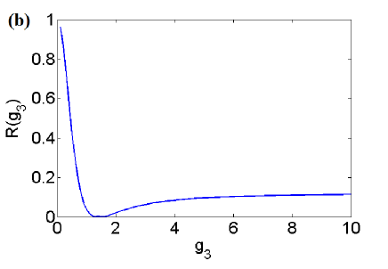
Figure 4: (Color online) Numerical solution of Eq.(2) for boundary conditions (8). (a) Total energy and time-dependence of the energy for each bond with $g_{1}=1,\;g_{2}=g_{3}=\sqrt{2}$. (b) Reflection coefficient as a function of $g_{3}$ for $g_{1}=1,\;g_{2}=\sqrt{2}$.

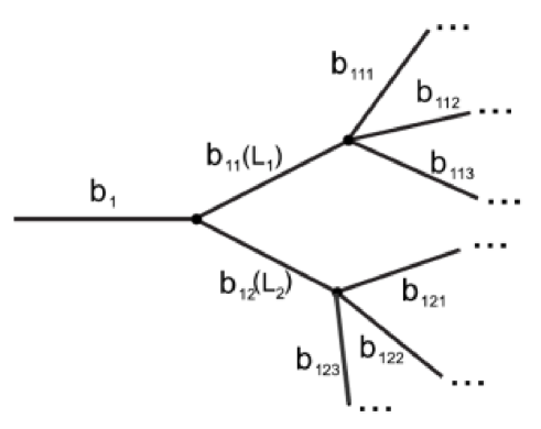
Figure 5: Tree graph. $x_{1}\in(-\infty,0],x_{1i}\in[0,L_{i}]$, and $x_{1ij}\in[0,+\infty)$ with $i=1,2;j=1,2,3$.

4 Extension for other graphs

The above treatment of the NLDE on the metric star graph can be extended to the tree graph presented in Fig. 5. It consists of three subgraphs $b_{1},(b_{1i}),(b_{1ij})$, where $i,j$ run over the given bonds of a subgraph. On each bond $b_{1},b_{1i},b_{1ij}$ we posit that the nonlinear Dirac equation is satisfied as given by Eq. (2). The vertex boundary conditions can be written similarly to those in Eq. (12). Soliton solutions have a similar form to those in Eqs. (13)-(14) where $x$ is replaced by $x+s_{b}$, with $s_{1}=s_{1i}=l,\,s_{1ij}=l+L_{i}$, with $l$ being position of the center of mass of soliton. The sum rules in this case generalize according to:

$$\frac{1}{g_{1}^{2}}=\sum_{i=1}^{2}\frac{1}{g_{1i}^{2}},\,\,\,\frac{1}{g_{1i}^{2}}=\sum_{j=1}^{3}\frac{1}{g_{1ij}^{2}},\,\,\,i=1,2.$$

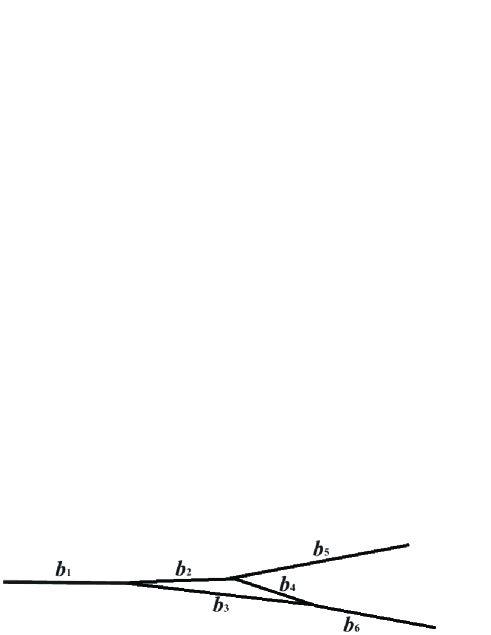
Figure 6: Triangle graph. $x_{1}\in(-\infty,0],x_{i}\in[0,L_{i}]$ with $i=2,3,4$, and $x_{j}\in[0,+\infty)$ with $j=5,6$.

Similarly to that for star graph, one can obtain soliton solutions of the nonlinear Dirac equation on the tree graph for the moving frame.

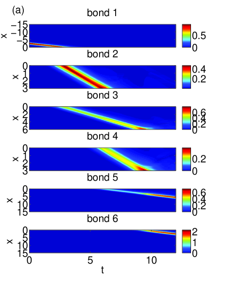
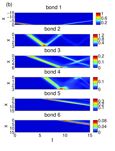
Figure 7: (Color online) Time and coordinate dependence of the charge density obtained from the numerical solution of Eq.(2) ($x_{0}=0$)for the case (a) when constraints (23)–(25) are fulfilled ($g_{1}=1,\;g_{2}=g_{3}=\sqrt{2},\;g_{4}=g_{5}=2,\;g_{6}=2/\sqrt{3}$), (b) when these constraints are not fulfilled ($g_{1}=g_{3}=g_{5}=1,\;g_{2}=g_{4}=g_{6}=2$).

Another graph for which a soliton solution of the nonlinear Dirac equation can be obtained, is presented in Fig. 6. It has the form of a triangle whose vertices are connected to outgoing semi-infinite leads. The vertex boundary conditions for Eqs. (10) and (11) which follow from the conservation of current and energy can be written as

$$\alpha_{1}\phi_{1}|_{x=0}=\alpha_{2}\phi_{2}|_{x=0}+\alpha_{3}\phi_{3}|_{x=0},$$

$$\frac{1}{\alpha_{1}}\chi_{1}|_{x=0}=\frac{1}{\alpha_{2}}\chi_{2}|_{x=0}=\frac{1}{\alpha_{3}}\chi_{3}|_{x=0},$$

$$\alpha_{2}\phi_{2}|_{x=L_{2}}=\alpha_{4}\phi_{4}|_{x=0}+\alpha_{5}\phi_{5}|_{x=0},$$

$$\frac{1}{\alpha_{2}}\chi_{2}|_{x=L_{2}}=\frac{1}{\alpha_{4}}\chi_{4}|_{x=0}=\frac{1}{\alpha_{5}}\chi_{5}|_{x=0},$$

$$\alpha_{3}\phi_{3}|_{x=L_{3}}+\alpha_{4}\phi_{4}|_{x=L_{4}}=\alpha_{6}\phi_{6}|_{x=0},$$

$$\frac{1}{\alpha_{3}}\chi_{3}|_{x=L_{3}}=\frac{1}{\alpha_{4}}\chi_{4}|_{x=L_{4}}=\frac{1}{\alpha_{6}}\chi_{6}|_{x=0}.$$

In short, the conditions matching the of charge and energy conservations must be applied to each node connecting the multiple vertices of the graph. The soliton solution obeying these boundary conditions can be written as

$$A_{b}(x)=\frac{1}{|g_{b}|}\cosh(\beta(x+s_{b}))\sqrt{\frac{m+\omega}{m+\omega\cosh(2\beta(x+s_{b}))}}$$

$$\times\sqrt{\frac{2\beta^{2}}{m+\omega\cosh(2\beta(x+s_{b}))}},$$

(21)

$$B_{b}(x)=\frac{1}{|g_{b}|}|\sinh(\beta(x+s_{b}))|\sqrt{\frac{m-\omega}{m+\omega\cosh(2\beta(x+s_{b}))}}$$

$$\times\sqrt{\frac{2\beta^{2}}{m+\omega\cosh(2\beta(x+s_{b}))}},$$

(22)

where $b$ is considered to be an index running from $1$ to $6$, $s_{1}=s_{2}=s_{3}=l,\,s_{4}=l+L_{2},\,s_{5}=l+L_{2},\,s_{6}=l+L_{3},\,L_{3}=L_{2}+L_{4}$ (this condition is necessary for the waves traveling along $b_{3}$ and those split along $b_{2}$ and $b_{4}$ to arrive at the vertex between $b_{3}$ and $b_{4}$ concurrently) and coefficients $g_{j}$ fulfill the following constraints:

$$\frac{1}{g_{1}^{2}}=\frac{1}{g_{2}^{2}}+\frac{1}{g_{3}^{2}},$$ (23)

$$\frac{1}{g_{2}^{2}}=\frac{1}{g_{4}^{2}}+\frac{1}{g_{5}^{2}},$$ (24)

$$\frac{1}{g_{3}^{2}}+\frac{1}{g_{4}^{2}}=\frac{1}{g_{6}^{2}}.$$ (25)

Again, the traveling wave (soliton) solutions can be obtained in case of the moving frame using the Lorentz transformations. This approach for designing soliton solutions of the nonlinear Dirac equation can be applied to other graph topologies with multiple junctions, provided a graph consists of finite parts connected to outgoing semi-infinite bonds.

In Fig. 7 the solution of NLDE on each bond of this triangle graph is plotted for the cases when the sum rule given by Eqs. (23)-(25) is fulfilled (a) and is broken (b). Absence of the vertex reflection in Fig. 7(a) is clearly seen, while in Fig. 7(b) the transmission of Dirac solitons through the graph vertices is clearly impeded by the mismatch at the VBC. Thus, reflection events are clearly discernible in bonds such as $1$, $3$ and $4$.

5 Conclusions & Future Challenges

In this paper we studied dynamics of Dirac solitons in networks by considering the case of metric graphs. We obtained soliton solutions of the nonlinear Dirac equation on some of the simplest metric graphs such as the star, tree and triangle graphs. Constraints enabling such exact solutions to exist are derived in the form of sum rules for bond nonlinearity coefficients. The boundary conditions at the branching points (vertices) are derived from the fundamental conservation laws. It is shown via direct numerical simulations that within the corresponding dynamics the obtained constraints provide for reflectionless transmission of solitary waves at the graph vertex. In the case where the relevant conditions are violated, nontrivial reflections ensue.

Our computations clearly suggest that the considered vertex boundary conditions are necessary (yet not necessarily sufficient) conditions for reflectionless transmission through the junctions of interest. This is also in line with the recent homogenization calculation of [54]. It is thus natural to formulate the following conjecture. Assume that the initial data correspond to a traveling wave of the NLDE in the form of Eq. (20) centered at $x_{0}$, with $v>0$. Then for $t\rightarrow+\infty$, the solution can consist asymptotically of a superposition of solitary waves in branches 2 and 3, only if the condition of Eq. (17) holds. This conjecture poses a challenging mathematical question for further rigorous study in the problem at hand, both at the level of the NLDE, but also by direct analogy in the context of the NLS and other similar models.

It should be noted that an important, additional set of challenges emerges as regards the study of stationary solutions involving the vertex. In the language of the very recent work of [54], the states considered herein are the so-called half-soliton states. Yet in the NLS framework of the latter work, additional so-called shifted (non-monotone in the different branches) states also exist, yet they may be spectrally unstable, depending on whether they are monotonic or non-monotonic in the outgoing edges of the metric graph. The half-soliton considered here is especially interesting as at the NLS level it turns out to be spectrally stable, yet nonlinearly unstable. This issue of the (more involved at the NLDE level [55]) spectral stability of these stationary states is also an especially interesting direction for future study.

Naturally, the above study can be extended for other simple topologies, such as a graph with one or multiple loops (e.g. the dumbbell graph), or other combinations of star, tree and loop graphs.

It will be extremely interesting if these ideas induce experimental interest in systems such as suitably tailored discrete optical waveguides [52, 53] or in atomic settings, in the same way as they have for instance for the propagation of traveling waves through networks of granular crystals [56].

6 Appendix A

Here we will show that the linear vertex boundary conditions given by Eqs. (8) lead to the ones given by (5)-(7). Consider the following (linear) relations given at the vertex of the a metric star graph

$$\alpha_{1}\phi_{1}|_{x=0}=\alpha_{2}\phi_{2}|_{x=0}+\alpha_{3}\phi_{3}|_{x=0},$$ (26)

$$\frac{1}{\alpha_{1}}\chi_{1}|_{x=0}=\frac{1}{\alpha_{2}}\chi_{2}|_{x=0}=\frac{1}{\alpha_{3}}\chi_{3}|_{x=0},$$ (27)

where $\alpha_{1},\,\alpha_{2},\,\alpha_{3}$ are real constants.

Multiplying both sides of Eq. (26) by $\frac{1}{\alpha_{1}}\chi_{1}^{*}|_{x=0},$ from Eq. (27) we have

$$\phi_{1}\chi_{1}^{*}|_{x=0}=\phi_{2}\chi_{2}^{*}|_{x=0}+\phi_{3}\chi_{3}^{*}|_{x=0}.$$ (28)

From Eq. (28) we get

$${\rm Re}[\phi_{1}\chi_{1}^{*}]|_{x=0}={\rm Re}[\phi_{2}\chi_{2}^{*}]|_{x=0}+{\rm Re}[\phi_{3}\chi_{3}^{*}]|_{x=0},$$ (29)

which is nothing but the vertex boundary condition given by Eq. (5). Taking the time derivative from Eq. (27) and multiplying both sides of (26) by $\frac{1}{\alpha_{1}}\partial_{t}\chi_{1}^{*}|_{x=0}$, we obtain

$$\phi_{1}\partial_{t}\chi_{1}^{*}|_{x=0}=\phi_{2}\partial_{t}\chi_{2}^{*}|_{x=0}+\phi_{3}\partial_{t}\chi_{3}^{*}|_{x=0}.$$ (30)

Taking the time-derivative from Eq. (26) and multiplying the complex conjugate of the obtained expression by $\frac{1}{\alpha_{1}}\chi_{1}|_{x=0}$ we get

$$\chi_{1}\partial_{t}\phi_{1}^{*}|_{x=0}=\chi_{2}\partial_{t}\phi_{2}^{*}|_{x=0}+\chi_{3}\partial_{t}\phi_{3}^{*}|_{x=0}.$$ (31)

Adding Eqs. (30) and (31) leads to

$$[\phi_{1}\partial_{t}\chi_{1}^{*}+\chi_{1}\partial_{t}\phi_{1}^{*}]|_{x=0} = [\phi_{2}\partial_{t}\chi_{2}^{*}+\chi_{2}\partial_{t}\phi_{2}^{*}]|_{x=0}$$ (32)

$$+ [\phi_{3}\partial_{t}\chi_{3}^{*}+\chi_{3}\partial_{t}\phi_{3}^{*}]|_{x=0}.$$

The last equation yields the vertex boundary condition given by Eq. (7).

References

- [1] Z. Sobirov, D. Matrasulov, K. Sabirov, S. Sawada, and K. Nakamura, Phys. Rev. E 81, 066602 (2010).
- [2] K. Nakamura, Z. A. Sobirov, D. U. Matrasulov, and S. Sawada, Phys. Rev. E 84, 026609 (2011).
- [3] R. Adami, C. Cacciapuoti, D. Finco, and D. Noja, Rev. Math. Phys. 23, 409 (2011).
- [4] R. Adami, C. Cacciapuoti, D. Finco, and D. Noja, Europhys. Lett. 100, 10003 (2012).
- [5] R. Adami, D. Noja, and C. Ortoleva, J. Math. Phys. 54, 013501 (2013).
- [6] K.K. Sabirov, Z.A. Sobirov, D. Babajanov, and D.U. Matrasulov, Phys. Lett. A, 377, 860 (2013).
- [7] D. Noja, Philos. Trans. R. Soc. A 372, 20130002 (2014).
- [8] G. H. Susanto and S.A. van Gils, Phys. Lett. A 338, 239 (2005).
- [9] J.-G Caputo , D. Dutykh, Phys. Rev. E 90, 022912 (2014).
- [10] H. Uecker, D. Grieser, Z. Sobirov, D. Babajanov, and D. Matrasulov, Phys. Rev. E 91, 023209 (2015).
- [11] Z. Sobirov, D. Babajanov, D. Matrasulov, K. Nakamura, and H. Uecker, EPL 115 , 50002 (2016).
- [12] W. Thirring, Ann. Phys. 3, 91 (1958).
- [13] D. J. Gross, A. Neveu, Phys. Rev. D 10, 3235 (1974).
- [14] W.H. Steeb, W. Oevel, and W. Strampp, J. Math. Phys. 25, 2331 (1984).
- [15] I. V. Barashenkov and B. S. Getmanov, Commun. Math. Phys. 112, 423 (1987).
- [16] W.I. Fushchych and R.Z. Zhdanov, J. Math. Phys. 32, 3488 (1991).
- [17] I. V. Barashenkov and B. S. Getmanov, J. Math. Phys. 34, 3054 (1992).
- [18] F.M. Toyama, Y. Hosono, B. Ilyas and Y. Nogami, J. Phys. A: Math. Gen. 27, 3139 (1994).
- [19] W.K. Ng, Int. J. Mod. Phys. A, 24, 3476 (2009).
- [20] W.K. Ng and R.R. Parwani, SIGMA 5, 023 (2009).
- [21] L. H. Haddad and L. D. Carr, Physica D 238, 1413 (2009).
- [22] L. H. Haddad and L. D. Carr, Europhys. Lett. 94 56002 (2011).
- [23] L.H. Haddad, C.M. Weaver and L.D Carr, New J. Phys. 17, 063033 (2015).
- [24] L.H. Haddad, L.D Carr, New J. Phys. 17, 063034 (2015).
- [25] L.H. Haddad, L.D Carr, New J. Phys. 17, 113011 (2015).
- [26] L.H. Haddad, K. M. O’Hara, L.D Carr, Phys. Rev. A 91, 043609 (2015).
- [27] F.Cooper, A. Khare, B. Mihaila and A. Saxena, Phys. Rev. E 82, 036604 (2010).
- [28] F. G. Mertens, N. R. Quintero, F. Cooper, A. Khare, and A. Saxena, Phys. Rev. E 86, 046602 (2012).
- [29] D.E. Pelinovsky, A.Stefanov, J. Math.Phys.,53, 073705 (2012).
- [30] D.E. Pelinovsky, Y. Shimabukuro, Lett. Mat. Phys.,104, 21 (2014).
- [31] S. Shao, F. G. Mertens, N. R. Quintero, F. Cooper, A. Khare, and A. Saxena, Phys. Rev. E 90, 032915 (2014).
- [32] J. Cuevas-Maraver, P.G Kevrekidis and A. Saxena, J. Phys. A: Math. Gen. 48, 055204 (2015).
- [33] F. G. Mertens, F. Cooper, N.R. Quintero, S. Shao, A. Khare, and A. Saxena, J. Phys. A: Math. Gen. 49, 065402 (2016).
- [34] J. Cuevas-Maraver, P.G. Kevrekidis and A. Saxena, F. Cooper, A. Khare, A. Comech, C.M.Bender, IEEE J. Selected Topics Quant. Electr.,22, 5000109 (2016).
- [35] J. Cuevas-Maraver, P.G Kevrekidis and A. Saxena, A.Comech, R.Lan, Phys. Rev. Lett. 116, 214101 (2016).
- [36] A. Contreras, D.E. Pelinovsky, Y. Shimabukuro, Commun. Part. Diff. Eq.,41, 227 (2016).
- [37] A. Komech, A. Komech, SIAM J. Math. Anal., 42, 2944 (2010).
- [38] G. Berkolaiko, A. Comech, Math. Mod. of Natural Phenomena, 7, 13 (2012).
- [39] A. Comech, M. Guan and S. Gustafson, Ann. Henri Poincare (Analyse non lineaire), 31 639 (2014).
- [40] G. Berkolaiko, A. Comech, A. Sukhtayev, Nonlinearity, 28 577 (2015).
- [41] J. Cuevas-Maraver, P.G. Kevrekidis, A. Saxena, A. Comech, R. Lan, Phys. Rev. Lett. 116 214101 (2016).
- [42] Y Zhang, Nonlinear Analysis, 118 82 (2015).
- [43] Ch-W. Lee, P. Kurzynski, H. Nha, Phys. Rev. A 92 052336 (2015).
- [44] T.X. Tran, X.N. Nguyen, F. Biancalana, Phys. Rev. A 91, 023814 (2008).
- [45] A.N. Andriotis, M. Menon, Appl.Phys.Lett., 92 042115 (2008).
- [46] Y.P. Chen, Y.E. Xie, L. Z. Sun and J. Zhong, Appl. Phys. Lett., 93 092104 (2008).
- [47] J. G. Xu, L. Wang and M. Q. Weng, J. Appl. Phys., 114 153701 (2013).
- [48] A.G. Kvashnin, D.G. Kvashnin, O.P. Kvashnina and L.A. Chernozatonskii, Nanotechnology, 26 385705 (2015).
- [49] T.X. Tran, S. Longhi, F. Biancalana, Ann. Phys. 340 179 (2014).
- [50] D.N. Christodoulides and E.D. Eugenieva Phys. Rev. Lett. 87, 233901 (2001)
- [51] J. Bolte and J. Harrison, J. Phys. A: Math. Gen. 36 2747 (2003).
- [52] M. Conforti, C. De Angelis, T. R. Akylas, and A.B. Aceves Phys. Rev. A 85 063836 (2012).
- [53] A. Marini, S. Longhi, and F. Biancalana Phys. Rev. Lett. 113 150401 (2014).
- [54] A. Kairzhan, D.E. Pelinovsky, J. Phys. A: Math. Theor. 51, 095203 (2018).
- [55] J. Cuevas-Maraver, N. Boussaid, A. Comech, R.Lan, P.G. Kevrekidis, A. Saxena, arXiv:1707.01946.
- [56] A. Leonard, L. Ponson, C. Daraio, J. Mech. Phys. Solids 73, 103 (2014).