Discrete Spectrum Reconstruction using Integral Approximation Algorithm

Abstract

An inverse problem in spectroscopy is considered. The objective is to restore the discrete spectrum from observed spectrum data, taking into account the spectrometer’s line spread function. The problem is reduced to solution of a system of linear-nonlinear equations (SLNE) with respect to intensities and frequencies of the discrete spectral lines. The SLNE is linear with respect to lines’ intensities and nonlinear with respect to the lines’ frequencies. The integral approximation algorithm is proposed for the solution of this SLNE. The algorithm combines solution of linear integral equations with solution of a system of linear algebraic equations and avoids nonlinear equations. Numerical examples of the application of the technique, both to synthetic and experimental spectra, demonstrate the efficacy of the proposed approach in enabling an effective enhancement of the spectrometer’s resolution.

1 Introduction

Spectral analysis is widely used for the qualitative and quantitative study of substancesl1 ; l2 ; l3 ; l4 ; l5 ; l6 . The spectrum $u(\nu)$ characterizes dependency of intensity of radiation as a function of frequency $\nu$. There are different types of spectra, including continuous, discrete, etc. playing principal role in scattering theory. There are various spectroscopic tools available for light decomposition into a spectruml2 .

Two possible avenues are available to increase the spectrometer’s resolution. The first avenue mainly concerns hardware, whereby engineers design a more sophisticated and expensive spectrometer. This paper follows the second avenue and employs mathematical processing of the measurements.

The purpose of this work is to propose a novel approach capable of restoring the discrete spectrum based on measured, possibly smoothed and noisy, spectral data and taking into account the spectrometer’s known line spread function. The problem is reduced to solution of a system of linear and nonlinear equations (some equations are linear in their variables, while some are not) using the integral approximation algorithm. The algorithm is implemented in Matlab. A discrete (or line) spectrum consists of discrete nearly monochromatic lines. The discrete spectrum is widely used to characterize diffuse interstellar nebulae, low temperature gas-discharge plasma and any substance in a deep vacuum.

Spectrum recovery (or deconvolution) is a well-known inverse problem in spectroscopy and belongs to the ill-posed category of problems. It is one of the variants of the classic Rayleigh reduction problem l1 ; l6 .

The conventional approach to attack this challenging inverse problem involves the Fourier self-deconvolution (FSD) technique l31 to enhance the resolution of spectral overlapping lines. The main idea of FSD is to employ the Fourier-transformed spectroscopy when the interferogram spectrum is measured followed by the Fourier transform. In order to enhance the resolution FSD uses apodization (truncation of the interferogram). The objective of FSD is overlapping lines separation, i.e. when the low resolution caused by lines proximity and width, but it is not caused by instrumental function’s width as in the present paper. It is to be noted that apodization causes lines widths artificial reduction, i.e. true lines profiles are distorted (to improve their resolution). In present paper (as well as in l6 , l8 ; l9 ; l10 ) the slightly different problem is addressed: effective enhancement of spectrometer’s resolution without artificial reduction of lines profiles.

2 Problem statement

Let $u(\nu)$ be a spectrum measured e.g. by a Fabry-Pérot interferometer l7 . The measured spectrum $u(\nu)$ is usually different from true spectrum $z(\nu)$ due to measurement errorsl6 ; l9 and the influence of the spectrometer’s instrumental functionl1 ; l5 ; l6 ; l8 ; l9 . The following definition of the instrumental functionl1 ; l5 ; l6 ; l8 ; l9 can be formulated.
Instrumental response function (IF, or spectral sensitivity, transmission function, point spead function, frequency response) $K(\nu,\nu^{\prime})$ is the spectrometer’s response (in terms of measured intensity) on a discrete line of unit intensity and frequency $\nu^{\prime}$ when the spectrometer is tuned to the desired frequency $\nu$ (proportional to a wavenumber). Fixing $\nu$ and changing $\nu^{\prime}$, the dependency $K(\nu,\nu^{\prime})$ can be obtained in the form of a curve as shown in Figure 1.

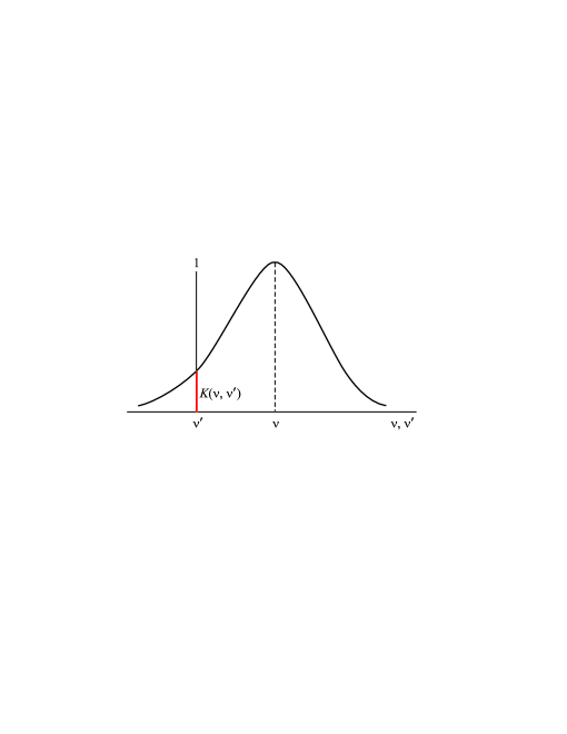
Figure 1: Dependency $K(\nu,\nu^{\prime})$ with concrete $\nu.$

Similar curves can be obtained for other values of $\nu$. The result is a two-dimensional function $K(\nu,\nu^{\prime})$. A wider instrumental function results in a smoother measured spectrum $u(\nu)$ when compared with the actual spectrum $z(\nu).$

The discrete spectrum $z(\nu)$ is composed of individual substantially monochromatic lines characterized by their frequencies and intensities (amplitudes). The problem of restoring the true discrete spectrum can be described by the following relationl6 ; l10 ; l11

$${\mathcal{A}}z\equiv\sum_{j=1}^{n}K(\nu_{i},\nu_{j}^{\prime})z_{j}+F=\tilde{u}({\nu}_{i}),\,i=\overline{1,m},\,$$ (1)

where $c\leq\nu_{i}\leq d,$ $z_{j}$ is intensity (amplitude) of $j$th line, $\nu_{j}^{\prime}$ is its frequency, $n$ is number of lines, $\nu_{i}$ is digital readout of frequency $\nu$ based on spectrometer tuning characteristics, $m$ is the number of such readouts, $[c,\,d]$ is frequency band; source function of Eq. 1 $\tilde{u}(\nu_{i})=u(\nu_{i})+\delta u(\nu_{i}),$ where $\delta u$ is a random component of measurement noise; $F$ is a deterministic noise component, and ${\mathcal{A}}$ is linear-nonlinear operator.

The functions $\tilde{u}(\nu_{i}),\,K(\nu,\nu^{\prime}),\nu_{i},c,d,m$ are known in system 1, and $z_{j}$ are the desired values. System 1 contains both linear and nonlinear equations, namely the system is linear with respect to $z_{j}$ and $F$ and nonlinear with respect to $\nu_{j}^{\prime}.$

System 1 can be considered as a system of nonlinear equations (SNE) and the known methodsl12 ; l13 for solution of SNEs such as the Newton-Kantorovich method, gradient, chords, gradient projection, to name a few, can be applied directly with or without imposing restrictions on the desired solution.

However, these methods do not take into account the specifics of the system of linear and nonlinear Eqs 1 (SLNE). As a result, these methods require high computing time and memory. Moreover, false lines may appear as result of nonlinear system roots. Finally, the number of true spectral lines $n$ remains unknown.

The alternative avenue is to employ the folowing methods for solution of the SLNE:

1. Prony methodl14 . It is suitable for SLNE with Vandermonde matrix only, that is when matrix $K(\nu,\nu^{\prime})$ varies along its lines with geometric progression. That is not the case for the matrix of system 1.

2. Peebles–Berkowitz algorithml15 . It approximates an IF with a Taylor series resulting in errors in the solutions.

3. Falkovich–Konovalov algorithml16 which is a cumbersome algorithm, difficult to implement and tune.

4. Golub-Mullen-Hegland methodl17 ; l18 ; l19 of variable projection. In this algorithm the Gauss-Newton method must be used to find the desired frequencies.

In l19 , SLNE 1 is solved as follows. First, some frequencies $\nu_{j}^{\prime}$ and $\nu_{i}$ are given, the amplitudes $z_{j}$ are determined by the Moore–Penrose pseudoinverse $z={\mathcal{A}}^{+}\tilde{u}.$ Then, the frequencies $\nu_{j}^{\prime}$ are approximated (refined) via solving the nonlinear least squares problem by the Gauss–Newton or Levenberg–Marquardt methods. Thus, the problem is solved as a linear–nonlinear system.

3 Integral approximation algorithm

In order to design an efficient algorithm for the solution of system 1 which takes into account its specifics, the integral approximation algorithml6 ; l10 ; l11 is employed in the present paper. The integral approximation algorithm has demonstrated its efficiency in number of signal processing problemsl10 ; l11 as well as in spectroscopyl6 . The essence of the algorithm is as follows.

The conventional approach for the solution of integral equations is to use the method of quadrature by integral approximation by the finite sum, i.e. the original continuous problem being reduced to a discrete problem. Here the inverse operation is suggested: the discrete problem 1 is replaced with an integral equation (IE) to be solved using the quadrature method on finer mesh sizes. This enables the estimation of frequencies using only linear operations with an accuracy that depends on using a small discretization step.

This algorithm is performed in four steps as follows.

1st step. Instead of system 1 the following linear Fredholm equation of the first kindl6 ; l8 ; l9 ; l10 ; l11

$$Az\equiv\int_{a}^{b}\tilde{K}(\nu,\nu^{\prime})z(\nu^{\prime})\,d\nu^{\prime}=\tilde{u}(\nu),\,\,\,c\leq\nu\leq d$$ (2)

is considered with respect to function $z(\nu^{\prime}),$ where $A$ is a linear integral operator. It is assumed that instead of an exact source $u$ and kernel $K$ an approximate $\tilde{u},$ $\widetilde{K}$ are given such as $||\tilde{u}-u||\leq\delta,$ $||\widetilde{K}-K||\leq\xi,$ where $\delta$ and $\xi$ are upper bounds of the errors in the source function $u$ and kernel $K$. The following statementl11 is valid for SLNE 1 and integral Eq. 2.

If $z(\nu^{\prime})$ in Eq. 2 is a generalized function consisting of sum of the Dirac delta-functions l20 $z(\nu^{\prime})=\sum_{j=1}^{n}z_{j}\delta(\nu^{\prime}-\nu_{j})$ and $a\rightarrow-\infty,$ $b\rightarrow\infty,$ then Eq. 2 is reduced to system 1 with $F\equiv 0,$ i.e. there is a mutual transition between SLNE 1 and Eq. 2.

2nd step. The solution of Eq. 2 is a known ill-posed probleml6 ; l20 ; l21 ; l22 ; l23 ; l24 ; l25 ; l26 ; l27 . It is to be noted that direct application of the quadrature method results in a so-called “saw”, thus rendering the method very unstablel6 ; l23 . Therefore, stable methods such as zero-order Tikhonov regularization methodl6 ; l20 ; l21 ; l22 ; l23 ; l24 ; l25 ; l26 ; l27 should be applied. Using the Tikhonov method we replace Eq. 2 with the following regularized equation

$$\alpha z_{\alpha}(\varphi)+\int_{a}^{b}R(\varphi,\nu^{\prime})z_{\alpha}(\nu^{\prime})\,d\nu^{\prime}=U(\varphi),$$ (3)

where $a\leq\varphi\leq b,$ $\alpha>0$ is a regularization parameter,

$$R(\varphi,\nu^{\prime})=R(\nu^{\prime},\varphi)=\int_{c}^{d}K(\nu,\varphi)K(\nu,\nu^{\prime})\,d\nu,$$ (4)

$$U(\varphi)=\int_{c}^{d}K(\nu,\varphi)\tilde{u}(\nu)\,d\nu.$$ (5)

For solution of integral Eq. 2 quadrature methods l6 ; l21 ; l22 ; l23 ; l26 can be applied by replacement of the integral with a finite sum leading to the system of linear algebraic equations (SLAE) ${A}{z}=\tilde{u}.$ In that case quadrature coefficients are assumed to be equal one in SLAE ${A}{z}=\tilde{u}$ to make it structurally close to SLNE 1. In order to obtain the stable solution instead of SLAE ${A}{z}=\tilde{u}$ we solve following stabilized SLAE which follows from Eqs. 3-5

$$(\alpha{E}+{A}^{T}{A}){z}_{\alpha}={A}^{T}\tilde{u}$$ (6)

with the square matrix ${R}=(\alpha{E}+{A}^{T}{A})$ of dimention $N\times N,$ where $N$ is the number of discrete samples for $\nu^{\prime},$ ${E}$ is the identity matrix, ${A}$ is a $m\times N$ matrix based on kernel $K;$ ${A}^{T}$ is the transposed matrix; $\tilde{u}$ is a given vector of length $m$ which is the measured spectrum. The desired solution of SLAE 6 is intensity vector ${z}_{\alpha j}\equiv{z}_{\alpha}(\nu_{j}^{\prime}),j=\overline{1,N}$ on a fine mesh with reduced step $h=\Delta\nu^{\prime}=(b-a)/(N-1).$

A critical matter is the strategy for the choice of the regularization parameter $\alpha$. The conventional method for choosing the parameter $\alpha$ is based on the Morozov discrepancy principle l28 . In this principle the parameter $\alpha$ can be chosen using equality (see Fig. 3 below)

$$||{A}{z}_{\alpha}-\tilde{u}||=\delta,$$ (7)

where the discrepancy $||{A}{z}_{\alpha}-\tilde{u}||$ can be written as follows

$$||{A}{z}_{\alpha}-\tilde{u}||_{2}:=\biggl{\{}\sum_{i=1}^{m}\biggl{[}\sum_{j=1}^{N}A_{ij}z_{\alpha j}-\tilde{u}_{j}\biggr{]}^{2}\biggr{\}}^{1/2}.$$ (8)

In Eq. 7 $\delta=||\tilde{u}-{u}||_{2},$ where $\tilde{u}$ is the measured noisy spectrum, and $u$ is the unknown non-noisy spectrum. Here $u$ is approximated by a smoothing spline through the noisy samples $\tilde{u}.$ Such an approach has been successfully employed in l25 ; l29 . $\alpha_{d}$ denotes a regularization parameter chosen according to the discrepancy principle.

The discretization step $h$ should be as small as possible in order to make several hundred discrete samples $N$ for $\nu^{\prime},$ i.e. $N\gg n,$ where $n$ is expected number of lines (see Eq. 1). The number $m$ for $\nu$ is the same as in Eq. 1, or it can be increased using the spline function. Employing a small discretization step $h$ is important in the application of this algorithm.

It is to be noted that $N\lessgtr m$, i.e. at any ratio of $N$ and $m$ the Tikhonov regularization method gives the solution (normal pseudo-solution) of the integral Eq. 3 and the corresponding SLAE. If $N$ is assumed to be greater than $m$ then, based on a limited number of measurements $m$ (e.g., $m\approx 100$), one can obtain a solution ${z}_{\alpha}(\nu^{\prime})$ defined on a greater number of nodes $N$ (e.g., $N\approx 400$) and using a smaller step $h=\Delta\nu^{\prime}.$

The desired solution ${z}_{\alpha}(\nu^{\prime})$ is thus obtained. Such a solution can help to distinguish the additional lines in the desired spectrum. False line-peaks may arise and must be filtered, and this issue is addressed below.

The following estimatel6 ; l9 ; l10 ; l11 of the error’s norm of the regularized solution ${z}_{\alpha}(\nu^{\prime})$ of Eq. 3 is carried out

$$\varepsilon(\alpha)\equiv||\Delta{z}_{\alpha}||\leq\left(\frac{||{A}||}{2\sqrt{\alpha}}\eta+\frac{p\alpha}{p\alpha+1}\right)||{z}_{\alpha}||,$$ (9)

where $\eta=\delta_{\text{rel}}+\xi_{\text{rel}},$ $\delta_{\text{rel}}=\delta/||{u}||,$ $\xi_{\text{rel}}=\xi/||{A}||$ are relative errors of input data, and parameter $p$ can be chosen using the model spectra processing methodl9 .

Let us estimate the error $\sigma_{\nu_{j}^{\prime}}$ of $j$-th line frequency $\nu_{j}^{\prime}.$ The solution ${z}_{\alpha}(\nu^{\prime})$ is expanded in a Taylor series in the neighborhood of frequency $\tilde{\nu}_{j}^{\prime}$ as follows

$${z}_{\alpha}(\nu^{\prime})\approx{z}_{\alpha}(\tilde{\nu}_{j}^{\prime})+\frac{1}{2}{z}_{\alpha}^{\prime\prime}(\tilde{\nu}_{j}^{\prime})\Delta_{j}^{2},$$ (10)

where ${z}_{\alpha}^{\prime\prime}(\tilde{\nu}_{j}^{\prime})=\frac{\partial^{2}{z}_{\alpha}(\nu^{\prime})}{\partial\nu^{\prime 2}}\bigl{|}_{\nu^{\prime}=\tilde{\nu}_{j}^{\prime}},$ $\Delta_{j}=\nu^{\prime}-\tilde{\nu}_{j}^{\prime}=\sigma_{\nu_{j}^{\prime}}.$ It is to be noted that ${z}_{\alpha}^{\prime}(\tilde{\nu}_{j}^{\prime})=0$ and ${z}_{\alpha}^{{}^{\prime\prime\prime}}(\tilde{\nu}_{j}^{\prime})\approx 0.$ That is the reason why series 10 should provide an accurate approximation of ${z}_{\alpha}(\nu^{\prime})$ in the $j$th line neighborhood. Here $\tilde{\nu}_{j}^{\prime}$ is the approximate frequency of the $j$th line corresponding to the some peak in the solution ${z}_{\alpha}(\nu^{\prime}),$ $\nu^{\prime}$ is some frequency value in the neighborhood of $\tilde{\nu}_{j}^{\prime},$ in particular, exact frequency $\nu_{j}^{\prime}$ value. From Eq. 10 as follows:

$$(\nu^{\prime}-\tilde{\nu}_{j}^{\prime})^{2}\approx\frac{2[{z}_{\alpha}(\nu^{\prime})-{z}_{\alpha}(\tilde{\nu}_{j}^{\prime})]}{{z}_{\alpha}^{\prime\prime}(\tilde{\nu}_{j}^{\prime})}$$ (11)

or using absolute values

$$|\nu^{\prime}-\tilde{\nu}_{j}^{\prime}|\approx\sqrt{\frac{2|{z}_{\alpha}(\nu^{\prime})-{z}_{\alpha}(\tilde{\nu}_{j}^{\prime})|}{|{z}_{\alpha}^{\prime\prime}(\tilde{\nu}_{j}^{\prime})|}}.$$ (12)

However, such an error estimate of the $j$th line frequency can not be employed because $\nu^{\prime},$ is not known, in particular, the exact value of frequency $\nu_{j}^{\prime}.$

A more constructive approach for frequency error estimation is to employ the norms. Let us make the notation $||{z}_{\alpha}(\nu^{\prime})-{z}_{\alpha}(\tilde{\nu}_{j}^{\prime})||=||\Delta{z}_{\alpha}||=\varepsilon(\alpha)$ and obtain the following estimate of the $j$th line frequency $\nu_{j}^{\prime}$ error using $\varepsilon(\alpha)$ estimate the norm of the regularized solutions

$$\sigma_{\nu_{j}^{\prime}}\approx\sqrt{\frac{2\varepsilon(\alpha)}{|{z}_{\alpha}^{\prime\prime}(\tilde{\nu}_{j}^{\prime})|}},$$ (13)

where $\varepsilon(\alpha)$ is calculated using Eq. 9.

Error $\sigma_{\nu_{j}^{\prime}}$ also grows due to the finite discretization step $h=\Delta\nu^{\prime}$ used for numerical solution of the integral Eq. 2. The error growth is approximately equal to $h/2.$ Finally, taking the square root of two error terms the following more accurate error estimate can be obtained

$$\sigma_{\nu_{j}^{\prime}}\approx\sqrt{\frac{2\varepsilon(\alpha)}{|z_{\alpha}^{\prime\prime}(\tilde{\nu}_{j}^{\prime})|}+\left(\frac{h}{2}\right)^{2}}.$$ (14)

Eq. 14 ${z}_{\alpha}^{\prime\prime}(\tilde{\nu}_{j}^{\prime})$ is an estimate of the second derivative of the regularized solution ${z}_{\alpha}(\nu^{\prime})$ for $\nu^{\prime}=\tilde{\nu}_{j}^{\prime},$ i.e. in the area of $j$th line. If $h={\text{const}},$ then

$${z}_{\alpha}^{\prime\prime}(\tilde{\nu}_{j}^{\prime})\approx\frac{{z}_{\alpha}(\tilde{\nu}_{j}^{\prime}-h)-2{z}_{\alpha}(\tilde{\nu}_{j}^{\prime})+{z}_{\alpha}(\tilde{\nu}_{j}^{\prime}+h)}{h^{2}}.$$ (15)

Estimate 14 shows that the determination error of frequencies $\sigma_{\nu_{j}^{\prime}}$ decreases as the discretization step $h=\Delta\nu^{\prime}$ decreases and as the second derivative $z_{\alpha}^{\prime\prime}(\tilde{\nu}_{j}^{\prime})$ increases, which increases with decreasing values of the regularization parameter $\alpha$. That is the reason why IE 3 should be solved using a small step $h$ and a small regularization parameter $\alpha.$

The following error metrics can be employed for analysis of the model spectrum with known exact intensities $z_{j}$ and frequencies $\nu_{j}^{\prime}$ $(j=\overline{1,n}).$

1. Root mean square error (RMSE) of lines’ intensities (cf. l27 ):

   $$\varepsilon=\biggl{\{}\frac{1}{n}\sum_{j=1}^{n}(\tilde{z}_{j}-z_{j})^{2}\biggr{\}}^{1/2}=||\tilde{z}-{z}||_{2},$$ (16)

2. RMSE of lines’ frequences:

   $$\xi=\biggl{\{}\frac{1}{n}\sum_{j=1}^{n}(\tilde{\nu^{\prime}}_{j}-\nu_{j}^{\prime})^{2}\biggr{\}}^{1/2}=||\tilde{\nu}^{\prime}-\nu^{\prime}||_{2}.$$ (17)

RMSE metrics depend on the system of units making them difficult to compare. The following relative root mean square errors (RRMSE) are used in our experiments:

$$\varepsilon_{\text{rel}}=\biggl{\{}\frac{\sum_{j=1}^{n}(\tilde{z}_{j}-z_{j})^{2}}{\sum_{j=1}^{n}z_{j}^{2}}\biggr{\}}^{1/2}=\frac{||\tilde{z}-{z}||_{2}}{||z||_{2}},$$ (18)

$$\xi_{\text{rel}}=\biggl{\{}\frac{\sum_{j=1}^{n}(\tilde{\nu^{\prime}}_{j}-\nu_{j}^{\prime})^{2}}{\sum_{j=1}^{n}\nu_{j}^{\prime 2}}\biggr{\}}^{1/2}=\frac{||\tilde{\nu}^{\prime}-\nu^{\prime}||_{2}}{||\nu^{\prime}||_{2}},$$ (19)

where $\tilde{z}_{j},$ $\tilde{\nu}_{j}^{\prime}$ are approximated intensities and frequencies, and ${z}_{j},$ ${\nu}_{j}^{\prime}$ are exact values of intensities and frequencies. Total RRMSE can be computed as follows:

$$\zeta_{\text{rel}}=\sqrt{\varepsilon_{\text{rel}}^{2}+\xi_{\text{rel}}^{2}}.$$ (20)

In the examples below the RMSEs $\varepsilon_{\text{rel}},$ $\xi_{\text{rel}},$ $\zeta_{\text{rel}}$ are employed.

3rd step. $L$ most powerful lines (maxima) are selected in the resulting solution $z_{\alpha}(\nu^{\prime})$ on the basis of additional information. Here $L$ is given with a margin such as $L\geq n,$ but $L\ll N,$ where $n$ is the expected number of lines. The frequencies of the most powerful maxima $\tilde{\nu}_{j}^{\prime},\,j=\overline{1,L}$ are recorded.

4th step. Solution of the following refined system of linear algebraic equations (SLAE) of lower order

$$\sum\limits_{j=1}^{L}K(\nu_{i},\tilde{\nu}_{j}^{\prime})\tilde{z}_{j}+\widetilde{F}=\tilde{u}(\nu_{i}),\,i=\overline{1,m},c\leq\nu_{i}\leq d.$$ (21)

This system has more equations than unknowns $\tilde{z}_{j},$ i.e. system 21 is overdetermined since $m>L.$ Usually, $m\sim 10^{2},L\sim 10^{1}$ and the least squares method (LSM) have to be used for such SLAE without regularisation with respect to line intensities $\tilde{z}_{j}$ and $\tilde{F}$ taking into account $\tilde{\nu}_{j}^{\prime}$ defined in Step 2 and 3. In the LSM the SLAE with a $(L+1)\times(L+1)$ square matrix is obtained. $\tilde{z}_{j}$ and $\tilde{F}$ are supposed to be chosen according to the following threshold

$$\tilde{z}_{j}\geq Z,\,j=\overline{1,k},\tilde{F}>0,$$ (22)

where $Z>0$ is the threshold value, and $k\leq L$ is the number of $\tilde{z}_{j}$ passing the threshold $Z.$ The threshold value can be chosen as follows l10 ; l11

$$Z=\delta\sqrt{-2\ln P_{\text{fa}}},$$ (23)

where $P_{\text{fa}}\in[0,\,1]$ is given conditional probability of a false alarm. However, false maxima are negative or nearly zero, so there is no need to use Eqs. 22, 23.

For sake of clarity let us summarize the algorithm.

Stage 1. IE. 2 is considered instead of SLNE 1.

Input: $\tilde{u}(\nu),n,m,c,d,K(\nu,\nu^{\prime}),a,b,h,\delta,N$.

Stage 2. IE 2 is solved using Tikhonov regularization (Eqs. 3 – 5) using reduced discretization step $h$ to get the SLAE (of $m$ equations) with respect to $N\gg n$ desired $z_{\alpha j}\equiv z_{\alpha}(\nu_{j}^{\prime}),$ where regularization parameter $\alpha$ is chosen using the Morozov discrepancy principle 7 – 8. The error of regularized solution is computed.

Output: $z_{\alpha}(\nu^{\prime}).$

Stage 3. Define $L$ maxima peaks in $z_{\alpha}(\nu^{\prime}),$ $L\geq n$ and $L\ll N.$

Output: frequencies $\tilde{\nu}_{j}^{\prime},j=\overline{1,L}.$

Stage 4. Refined SLAE 21 of lower order $m\times(L+1)$ is solved to find lines intensities $\tilde{z}_{j}$ and background $\tilde{F}$ using Eq. 22.

Output: lines intensities $\tilde{z}_{j}$, background $\tilde{F}$ and lines number $k$.

The advantage of the algorithm is that it allows linearization of the nonlinear problem of determination of the frequencies of spectral lines $\tilde{\nu}_{j}^{\prime}$ using the linear IE 2.

4 Numerical experiment

The proposed algorithm for discrete spectrum reconstruction is implemented as a software package in Matlab. In this section the package is tested on both model (for testing and verification) spectra and real spectra.

4.1 1st example: model spectrum

Following paperl9 , IF $K$ is assumed to have a variable width depending on frequency $\nu,$ i.e. in general the IF is not a convolution type kernel and $K=K(\nu,\nu^{\prime}).$ Such IFs are typical in broadband spectroscopy. The function $\tau(\nu)$, the half-width of the IF on half-power, is conventionally used. It is proportional to wavelength $\lambda$ and inversely proportional to the frequency, i.e. $\tau(\nu)=q/\nu,$ where the coefficient $q$ numerically determines the half-width of the IF and depends on the particular spectrometer design and setup.

The following most typical IFsl1 ; l9 ; l19 have been considered. These IFs are characterized by their half-widths $\tau(\nu)$ due to diffraction, aberrations and slots types.

1. Slotlike (rectangular) IF characterized by wide slot only

$$K(\nu,\nu^{\prime})=\left\{\begin{array}[]{ll}\frac{1}{2\tau(\nu)},&\hbox{if}|\nu-\nu^{\prime}|\leq\tau(\nu),\\ 0,&\hbox{otherwise}.\end{array}\right.$$ (24)

2. Triangular IF (also takes into account slit distortions only, it is the convolution of two rectangular IFs)

$$K(\nu,\nu^{\prime})=\left\{\begin{array}[]{l}\frac{1}{2\tau(\nu)}\left(1-\frac{|\nu-\nu^{\prime}|}{2\tau(\nu)}\right),\,\hbox{if\,}|\nu-\nu^{\prime}|\leq 2\tau(\nu),\\ 0,\,\hbox{otherwise.}\end{array}\right.$$ (25)

3. Rayleigh diffraction IF (in this case device has an infinitely narrow slot and the IF is determined by diffraction at a rectangular aperture diaphragm)

$$K(\nu,\nu^{\prime})=\frac{1}{\gamma(\nu)}\left\{\frac{\sin[\pi(\nu-\nu^{\prime})/\gamma(\nu)]}{\pi(\nu-\nu^{\prime})/\gamma(\nu)}\right\}^{2},$$ (26)

where $\gamma(\nu)=2\tau(\nu)/0.8859=2.2576\tau(\nu).$

4. Gaussian IFl6 ; l20 ; l30 (monochromator case where the diffraction and aberration distortions are not very large)

$$K(\nu,\nu^{\prime})=\frac{1}{\sqrt{2\pi}\sigma(\nu)}\exp\left(-\frac{(\nu-\nu^{\prime})^{2}}{2\sigma^{2}(\nu)}\right),$$ (27)

where $\sigma(\nu)=\tau(\nu)/\sqrt{2\ln 2}=0.8494\tau(\nu)$l6 .

5. Dispersion or Lorenz IF (for spectrographs of small, medium and sometimes large dispersion)

$$K(\nu,\nu^{\prime})=\frac{\tau(\nu)/\pi}{(\nu-\nu^{\prime})^{2}+\tau^{2}(\nu)}.$$ (28)

6. Exponential IF (of photosensitive layer)

$$K(\nu,\nu^{\prime})=\frac{\ln 2}{2\tau(\nu)}\exp\left(-\frac{\ln 2}{\tau(\nu)}|\nu-\nu^{\prime}|\right).$$ (29)

7. Voigt IF (convolution of Gauss and Dispersion IFs)l32 . Its explicit formula is omitted for the sake of brevity.

Remark.
Obviously IFs can also be written in terms of wavelength $\lambda$ (wavenumber $\nu/c=1/\lambda$), e.g. Eq. 29 can be writtenl9 as

$$K(\lambda,\lambda^{\prime})=\frac{\ln 2}{2\tau(\lambda)}\exp\left(-\frac{\ln 2}{\tau(\lambda)}|\lambda-\lambda^{\prime}|\right),$$ (30)

where $\tau(\lambda)=q\lambda$ is half-width of IF on half-power.

It is useful to employ the half-widths $\tau(\nu)$ when it comes to comparison of IFs with the same $\tau(\nu).$ Such a comparison was conductedl9 for continuous spectra. It is demonstrated that the most accurate results can be achieved for dispersion and exponential IFs and the least accurate results were achieved for slot and triangular IFs. This observation arose from processing the discrete spectra with various IFs 24-29 using the integral approximation algorithm.

Application of the integral approximation algorithm to the discrete spectrum described above confirmed this observation.

In order to demonstrate the efficiency of the proposed approach the following model examplel6 ; l10 ; l11 with synthetic data is considered in this section.

The true spectrum is given as seven discrete spectral lines with the following amplitudes (in arbitrary units, a.u.) $z_{1}=4.4,$ $z_{2}=4.6,$ $z_{3}=1.1,$ $z_{4}=3.2,$ $z_{5}=3.2,$ $z_{6}=2.8,$ $z_{7}=3.6$ and frequencies (given in a.u. as well) $\nu_{1}^{\prime}=2.28,$ $\nu_{2}^{\prime}=2.36,$ $\nu_{3}^{\prime}=2.95,$ $\nu_{4}^{\prime}=3.02,$ $\nu_{5}^{\prime}=3.56,$ $\nu_{6}^{\prime}=3.64,$ $\nu_{7}^{\prime}=3.69.$ The spectrometer’s IF is givenl9 as the following frequency–non-invariant Gaussian function (by Eq. 27), in which width decreases with increasing frequency $\nu$

$$K(\nu,\nu^{\prime})=\frac{g}{\sqrt{2\pi}\sigma(\nu)}\exp\left(-\frac{(\nu-\nu^{\prime})^{2}}{2\sigma^{2}(\nu)}\right),$$ (31)

where $\sigma(\nu)=\sigma_{0}\sqrt{1-0.16\nu},\sigma_{0}=0.05,$ $g=0.075$ is a normalizing factor, all in a.u. For each kind of spectrometer $\sigma(\nu),\,\sigma_{0}$ and $g$ will be specific. The level of the deterministic noise $F$ was assumed to be equal $0.2$, and the random measurement noise has a standard deviation (SD) equal to $0.05$ ($\approx 2\%$ noise).

The limits were selected as follows $a=c=2,$ $b=d=4$ a.u. (see Eqs. 2-5), $m=101$ is the number of “experimental” samples on $\nu$ (see Eq. 1); $N=401$ is the number of samples on $\nu^{\prime}$ in the SLAE 6 solution, discretization step $h=\Delta\nu^{\prime}=(b-a)/(N-1).$

Figure 2 shows: the true discrete (line) spectrum $z(\nu)$ consisting of 7 lines, the measured (experimental) noise free spectrum $u(\nu)$, the noisy spectrum $\tilde{u}(\nu),$ and the cubic spline approximation $\tilde{u}(\nu)$ is realised (length $m=101$).

In addition, the IF of the spectrometer $K(\nu,\nu^{\prime})$ according to Eq. 12 is given at low and high frequencies $\nu$. It can be observed that the true spectrum $z(\nu)$ has closely spaced lines (two lines coorresponding low frequency in Figure 2, two lines are in the middle and three lines corresponding high frequency) which remains unrecognized in the measured spectrum $u(\nu)$.

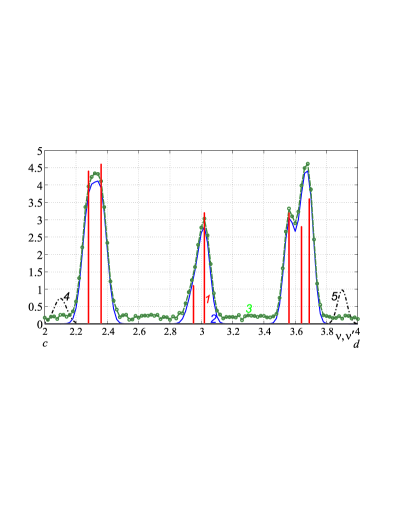
Figure 2: Numerical example of the direct problem. Frequencies $\nu$ and $\nu^{\prime}$ are located on the horizontal axis, $z,u,\tilde{u},$ and $K$ are on the vertical axis in a.u. “1” is the true discrete spectrum, “2” is the measured spectrum ${u}(\nu),$ “3” is the measured noisy spectrum $\tilde{u}(\nu),$ (dashed) and smoothing spline (circles) “4” is the IF $K(2.1,\nu^{\prime})$ on low frequency $\nu$, “5” is $K(3.9,\nu^{\prime})$ is the IF on high frequency $\nu$.

In this experiment the integral approximation algorithm is applied for the true spectrum. First, IE 2 is supposed to be solved using the Tikhonov regularization method following Eqs. 3-5 by means of the SLAE 6 solution. The regularization parameter $\alpha$ is chosen using the discrepancy principle 7 - 8 with $\alpha=\alpha_{d}=10^{-1.4}=0.04$ as shown in Fig. 3.

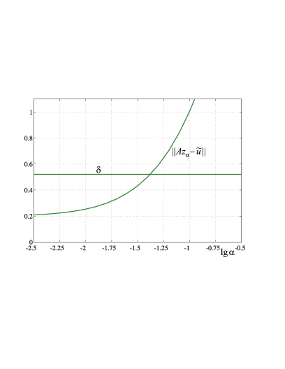
Figure 3: Discrepancy principle for specifying the regularization parameter $\alpha$.

Fig. 4 shows the noisy spectrum $\tilde{u}(\nu)$ according to Eq. 1 for $m=101,$ i.e. for relatively small (insufficient) samples $m.$

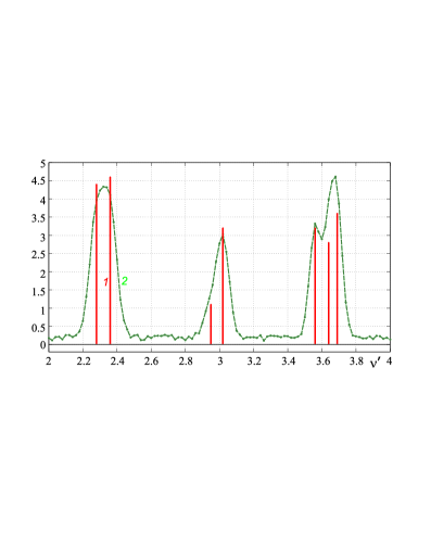
Figure 4: Measured and exact spectra. “1” is the exact spectrum ${z}(\nu^{\prime})$ (vertical solid lines); “2” is the measured spectrum $\tilde{u}(\nu)$ of length $m=101.$

Using the spectrum $\tilde{u}(\nu)$ of length $m=101$ the regularized solution ${z}_{\alpha}(\nu)$ is obtained, its length $N=401$ for $\alpha=\alpha_{d}$ (see Fig. 5). One may observe here the lack of resolution (the two rightmost high frequency lines are missing), so steps 3 and 4 of the integral approximation algorithm are not carried out.

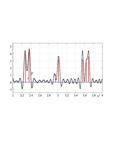
Figure 5: Numerical example. Inverse problem with insufficient $m=101.$ “1” is the true spectrum $z(\nu^{\prime})$ (vertical solid lines); “2” is the regularized solution $z_{\alpha}(\nu^{\prime})$ of length $N=401.$

In order to increase the effective resolution a cubic spline ${u}_{s}(\nu)$ of length $m=401$ is used to approximate the measured spectrum $\tilde{u}(\nu)$ as shown in Fig. 6.

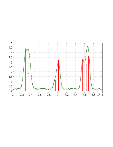
Figure 6: Measured and exact spectra. Here “1” is the exact spectrum ${z}(\nu^{\prime})$ (vertical solid lines); “2” is a smoothing spline ${u}_{s}(\nu)$ of length $m=401.$

The spline $u_{s}(\nu)$ of length $m=401$ is used to approximate the measured spectrum $\tilde{u}(\nu).$ Then the regularized solution is calculated using $\alpha=\alpha_{d}$ (see. Fig. 7).

It can be observed that in spite of the fact that in Fig. 7 the length of the solution is the same as in Fig. 5 ($N=401$), the resolution is improved significantly. This is due to the fact that the length of the measured spectrum $m$ is increased by using the spline.

In the regularized solution $z_{\alpha}(\nu)$ in Fig. 7 the first $L=12$ most powerful highs are taken and their frequences $\tilde{\nu}_{j}^{\prime},$ $j=\overline{1,L}$ are recorded. Then the refining SLAE 21 is solved using LSM (without regularization) with respect to $L+1=13$ unknowns: 12 amplitudes $\tilde{z}_{j}$ and $F$. Figure 7 shows the reconstructed spectrum values $z_{j}(\tilde{\nu}_{j}^{\prime})$. It is to be noted that all the false spectral lines correspond to negative values or values close to zero. Here the threshold value $Z=0.2F$ (20%), which has not been used. The true maximum values $\tilde{z}_{j}$ are indeed very close to the true amplitudes $z_{j}.$ The RRSME errors are $\varepsilon_{\text{rel}}=0.0621,$ $\xi_{\text{rel}}=0.0028$ and $\zeta_{\text{rel}}=0.0622.$

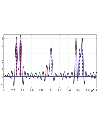
Figure 7: Numerical example of the inverse problem with increased $m=401.$ The frequency $\nu^{\prime}$ lies on the horizontal axis, $z$ is on the vertical axis in a.u. “1” is the true discrete spectrum ${z}(\nu^{\prime})$ (vertical solid lines), “2” is the regularised solution ${z}_{\alpha}(\nu^{\prime})$ of length $N=401$ (solid line); “3” is the reconstructed spectrum ${z}_{j}(\tilde{\nu}_{j}^{\prime})$ (vertical dashed lines).

All the 7 spectral lines have been perfectly recognized as well as their frequencies $\tilde{\nu}_{j}^{\prime}$ and intersities $\tilde{z}_{j}$ in the model example. This was achieved despite the noise and the IF which was selected to demonstrate the efficiency of the integral approximation algorithm.

For sake of comparison let us now solve this synthetic example using the variable projection Golub-Mullen-Hegland methodl17 ; l18 ; l19 . The efficient implementation of variable projection methodaddref (function varpro.m) was employed. Following notationsaddref , it’s assumed Ind = dPhi = [] which means that the derivatives (Jacobian matrix) were not used for solving both linear and nonlinear problems. This can reduce the accuracy of the solution, but simplifies the solution procedure. The problem was addressed using three versions as follows.

In the 1st version the uniform mesh was used on $\nu$=[2:0.1:4], number of nodes $m=21.$ Initial guess $\nu^{\prime}$=[2.26, 2.38, 2.93, 3.04, 3.54, 3.63, 3.71], number of lines $n=7.$ Resulting $z$ and $\nu^{\prime}$ are listed in the table below. The significant error can be observed especially in linear parameters $z$ (lines intensities). Apparently such error is caused by missing initial guess in the function varpro.m.

In the 2nd version the non-uniform mesh was used on $\nu$=[2.1; 2.2; 2.25; 2.3; 2.35; 2.4; 2.5; 2.6; 2.8; 2.9; 2.95; 3; 3.05; 3.1; 3.2; 3.3; 3.4; 3.5; 3.55; 3.6; 3.65; 3.7; 3.75; 3.8; 3.9], number of nodes $m=25.$ Initial guess for $nu^{\prime}$ was selected same as in the 1st version as described above. Table 1 demonstrates errors reduction and they are close to errors of the integral approximation algorithm: $\varepsilon_{\text{rel}}=0.0621,$ $\xi_{\text{rel}}=0.0028$ and $\zeta_{\text{rel}}=0.0622.$

The true number of spectral lines is normally remains not known. That’s the reason why in the 3rd version we assumed $n=9$ (instead of true $n=7$). Initial guess $\nu^{\prime}$ = [2.1, 2.26, 2.38, 2.93, 3.04, 3.1, 3.54, 3.63, 3.71] (two additional lines were introduced). The no-nuniform mesh was selected same as in the 2nd version. In order to calculate errors $\varepsilon_{\text{rel}},$ $\xi_{\text{rel}}$ and $\zeta_{\text{rel}}$ based on Eqs. 18 -20 two false lines with zero intensities were considered: $z$=[0; 4.4; 4.6; 1.1; 3.2; 0; 3.2; 2.8; 3.6], $\nu^{\prime}$=[2.1; 2.28; 2.36; 2.95; 3.02; 3.1; 3.56; 3.64; 3.69]. Table 1 shows that the intensities $z$ of false lines are correspondingly equal to 0.407 and 0.767, although one would expect near-zero values. It can be concluded that the false lines suppression does not work here.

1st version	error
$z:$ 6.413, 3.195, 1.155, 4.421, 1.467, 12.09, 0.682	$\varepsilon_{\text{rel}}=1.1272$
$\nu^{\prime}:$ 2.279, 2.417, 2.863, 3.026, 3.465, 3.652, 3,847	$\xi_{\text{rel}}=0.0257$
Warnings: linear parameters are not well-determined	$\zeta_{\text{rel}}=1.1275$
Number of iterations $N=28,$ time $T=1.5$ sec.
2nd version
$z:$ 4.848, 4.783, 1.361, 3.546, 3.271, 3.607, 3.498	$\varepsilon_{\text{rel}}=0.1146$
$\nu^{\prime}:$ 2.280, 2.363, 2.943, 3.020, 3.554, 3.638, 3.696	$\xi_{\text{rel}}=0.0014$
Warnings: there are no.	$\zeta_{\text{rel}}=0.1146$
$N=5,$ $T=0.3$ sec.
3rd version
$z:$ 0.407, 4.859, 4.743, 1.302, 3.555, 0.767, 3.271, 3.607, 3.498	$\varepsilon_{\text{rel}}=0.1481$
$\nu^{\prime}:$ 2.141, 2.280, 2.363, 2.941, 3.019, 3.145, 3.554, 3.638, 3.696	$\xi_{\text{rel}}=0.0069$
Warnings: there are no.	$\zeta_{\text{rel}}=0.1483$
$N=7,$ $T=0.4$ sec.

Table 1. Results of the variable projection method of Golub-Mullen-Hegland.

Hereby we can make the following preliminary conclusions.

1. The variable projection method requires a good initial guess for $\nu^{\prime}$, as well as the mesh for $\nu$ must be fine enough. It is to be noted that for the a real experiments it is technically difficult to employ the fine mesh. It is desirable to use derivatives (Jacobi matrix), but this makes the method complicated. Finally, it is not easy to a priory estimate the number $n$ of spectral lines. But the false lines are slightly suppressed.

2. The algorithm of integral approximation does not use an initial guess for $\nu^{\prime}$, but it also requires the fine mesh (for $\nu^{\prime},$ which is easy to generate). The question of the true number of spectral lines is solved reliably, since the false line are safely filtered (see. Fig. 7).

In general, the two methods complement each other. The main difference is that integral approximation is entirely linear method while variable projection is a linear-nonlinear method.

4.2 2nd example: real spectrum

It is to be noted that in this example wavelength $\lambda$ is used instread of frequency $\nu.$ Fig. 8 demonstrates the noisy spectrum of $\tilde{u}(\lambda)$ (20% concentration of carbon monoxide CO (IRT themes) heated to a temperature of $700\,^{\circ}{\rm C}$). The dataset is provided by Dept. Chem. and Biochem. Engg of DTU. In this example we have the Dispersion type IFl9 (cf. Eq. 28) as follows

$$K(\lambda,\lambda^{\prime})=\frac{a(\lambda)/2\pi}{(\lambda-\lambda^{\prime})^{2}+[a(\lambda)/2]^{2}},$$ (32)

where $a(\lambda)=q\lambda$ is the width of the instrumental function to half-power points, $q=0.0005$ such as $a(4780\,\text{nm})=2.4\,\text{nm}.$

The following integral equation (cf. Eq. 2) is solved

$$Az\equiv\int_{a}^{b}K(\lambda,\lambda^{\prime})z(\lambda^{\prime})\,d\lambda^{\prime},\,c\leq\lambda\leq d,$$ (33)

the desired function $z(\lambda^{\prime})$ is found using the quadrature method combined with the regularization method (given by Eqs. 3 – 6) for $a=4750,$ $b=4810,$ $c=4748,$ $d=4812,$ $N=301,$ $m=321,$ $h=0.2,$ $\alpha=\alpha_{d}=10^{-2}.$ As solution to SLAE Eq. 6 the regularized spectrum ${z}_{\alpha}(\lambda^{\prime})$ is obtained (curve “2” in Fig. 8).

Wavelengths $\tilde{\lambda}_{j}^{\prime}$ which correspond to the highest peaks (for $L=15$) are selected from the solution $z(\lambda^{\prime})$.

The SLAE (cf. Eq. 21)

$$\sum_{j=1}^{L}K(\lambda_{i},\tilde{\lambda}_{j}^{\prime})\tilde{z}_{j}+\tilde{F}=\tilde{u}(\lambda_{i}),i=\overline{1,m},\,c\leq\lambda_{i}\leq d$$ (34)

is solved, making it possible to refine amplitudes $\tilde{z}_{j}.$ The result is more accurate, see for example the vertical lines “3” in Fig. 8.

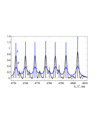
Figure 8: Real discrete spectrum. “1” is measured noisy spectrum $\tilde{u}(\lambda)$; “2” is the spectrum ${z}_{\alpha}(\lambda^{\prime})$ obtained by the regularized quadrature method; “3” is the reconstructed discrete spectrum ${z}_{j}(\tilde{\lambda}_{j}^{\prime}).$

Based on the experience gained from this approach to solution of the problem, it can be concluded that 7 largest lines have been safely recovered as well as 5 further weaker lines which have not been resolved in the measured spectrum $\tilde{u}(\lambda)$ (see curve 1 in Fig. 8). As for the three weakest peaks in the high frequency part of the spectrum $z_{\alpha}(\lambda^{\prime})$, two of them have negative values, but in the case of the maximum at $\lambda=4800$ it is difficult to judge whether it corresponds to real (weak) lines or to lines generated by the Gibbs phenomena.

5 Conclusion

We considered the problem of effective enhancement of spectrometer resolution without lines width artificial reduction. The experiment with synthetic and real data have demonstrated the high efficacy of the proposed method. A substantial increase in the effective resolution of the spectrometer was observed. The method enables enhancement of the resolution of spectral analysis through secure detection of closely located lines, detection of weak lines in noisy spectra, revealing the fine structure of reconstructed discrete spectra using mathematical and computer methods for spectral data processing.

The proposed algorithm enjoy affordable computational complexity, elapsed time was about 1 sec in both examples. It can be implemented as an embedded software system within a spectrometer in order to deliver higher effective resolution. Furthermore, an inexpensive spectrometer with a wide IF can be used combined with customised stand-alone Matlab software in order to enhance the original spectrometer’s effective resolution.

As a final remark it may be noted that the proposed algorithm for solving this inverse spectroscopy problem is a generic approach for analysing discrete spectra. It can be used to recover smoothed and noisy spectra in various applications including spectroscopy of gases, liquids, plasma and space objects, LiDARs, NMR spectroscopy, spectroscopic analysis of molten metal in blast furnaces etc.

The authors are grateful to the journal’s referees for their comments on an earlier draft, to Alexander Fateev (Dept. Chem. and Biochem. Engineering of DTU) for spectra measurements and to Paul Leahy (University College Cork) for helpful discussions.

This work was funded by Russian Foundation of Basic Research project No. 13-08-00442 and by the International science and technology cooperation program of China, project 2015DFR70850, NSFC Grant No. 61673398.

References

- (1) S.G. Rautian. “Real Spectral Apparatus”. Sov. Phys. Usp. 1958. 1(2): 245–273. doi:10.1070/PU1958v001n02ABEH003099.
- (2) P. Bousquet. Spectroscopy and its Instrumentation. London: Hilger Publ., 1971.
- (3) J. Workman Jr., A.W. Springsteen, eds. Applied Spectroscopy: A Compact Reference for Practitioners. San Diego: Academic Press, 1998.
- (4) J.M. Chalmers, P.R. Griffiths, eds. Handbook of Vibrational Spectroscopy. New York: Wiley, 2001. doi:10.1002/0470027320.
- (5) T. Fleckl, H. Jäger, I. Obernberger. “Experimental Verification of Gas Spectra Calculated for High Temperatures Using the HITRAN/HITEMP Database”. J. Physics D: Applied Physics. 2002. 35(23): 3138–3144. doi:10.1088/0022-3727/35/23/315.
- (6) V.S. Sizikov. Integral Equations and MATLAB in Problems of Tomography, Iconics and Spectroscopy, Saarbrücken: LAP (LAMBERT Academic Publishing), 2012.
- (7) J.K. Kauppinen, D.J. Moffatt, H.H. Mantsch, D. G. Cameron. ”Fourier Self-Deconvolution: A Method for Resolving Intrinsically Overlapped Bands”. Appl. Spectrosc. 1981. 35(3): 271–276.
- (8) S.G. Lipson, H. Lipson, D.S. Tannhauser. Optical Physics, 3rd ed. Cambridge University Press, 1995.
- (9) J.E. Stewart. “Resolution Enhancement of X-ray Fluorescence Spectra with a Computerized Multichannel Analyzer”, Appl. Spectrosc. 1975. 29(2): 171–174.
- (10) V.S. Sizikov, A.V. Krivykh. “Reconstruction of continuous spectra by the regularization method using model spectra”. Optics and Spectrosc. 2014. 117(6): 1010–1017. doi:10.1134/S0030400X14110162.
- (11) V.S. Sizikov. “Generalized Method for Measurement Data Reduction”. I. Processing of Tonal (Narrow-Band) Signals. Electron. Modeling (Gordon & Breach). 1992. 9(4): 618–633.
- (12) V. Sizikov. “Use of an integral equation for solving special systems of linear-non-linear equations”// In: Integral Methods in Science end Engineering. Vol. 2: Approximation Methods / C. Constanda, J. Saranen, S. Seikkala (eds.). Harlow: Longman, 1997. 200–205.
- (13) D.M. Himmelblau. Applied Nonlinear Programming. New York: McGraw-Hill, 1972.
- (14) W.C. Rheinboldt. Methods for Solving Systems of Nonlinear Equations, 2nd ed. Rhiladelphia: SIAM, 1998.
- (15) S.M. Kay, S.L. Marple. “Spectrum Analysis – A Modern Perspective”. Proc. IEEE. 1981. 69(11): 5 -51. doi:10.1109/PROC.1981.12184.
- (16) P. Peebles, R. Berkowitz. “Multiple-target monopulse radar processing techniques”. IEEE Trans. on Aerospace and Electronic Systems. 1968. AES-4(6): 845–854.
- (17) S.E. Falkovich, L.N. Konovalov. “Estimation for unknown numbers of signals”. J. Commun. Technol. Electron. 1982. 27(1): 92 -97.
- (18) G.H. Golub, V. Pereyra. “The Differentiation of Pseudo-Inverses and Nonlinear Least Squares whose Variables Separate”. SIAM J. Numer. Anal. 1973. 10(2): 413–432.
- (19) K.M. Mullen, I.H.M. van Stokkum. “The variable projection algorithm in time-resolved spectroscopy, microscopy and mass spectrometry applications”. Numer. Algor. 2009. 51(3): 319–340. doi: 10.1007/s11075-008-9235-2.
- (20) M. Hegland.“Error Bounds for Spectral Enhancement which are Based on Variable Hilbert Scale Inequalities”, J. Integral Equations Applications. 2010. 22(2): 285- 312, doi: 10.1216/JIE-2010-22-2-285.
- (21) D. Sidorov. Integral Dynamical Models: Singularities, Signals and Control, Singapore: World Sci. Publ., 2015. doi: 10.1142/9789814619196_0013.
- (22) A.N. Tikhonov, V.Ya. Arsenin. Solutions of Ill-Posed Problems. New York: Wiley, 1977.
- (23) H.W. Engl, M. Hanke, A. Neubauer. Regularization of Inverse Problems. Dordrecht: Kluwer, 1996.
- (24) Yu.P. Petrov, V.S. Sizikov. Well-Posed, Ill-Posed, and Intermediate Problems. Leiden–Boston: VSP, 2005.
- (25) Yu.E. Voskoboynikov, N.G. Preobrazhensky, A.I. Sedel nikov. Mathematical Treatment of Experiment in Molecular Gas Dynamics. Novosibirsk: Nauka, 1984.
- (26) V.S. Sizikov, D.N. Sidorov. Generalized quadrature for solving singular integral equations of Abel type in application to infrared tomography . Appl. Numer. Math. (Elsevier). 2016. 106: 69–78. doi: 10.1016/j.apnum.2016.03.004.
- (27) A.N. Tikhonov, A.N. Goncharsky, V.V. Stepanov, A.G. Yagola. Numerical Methods for the Solution of Ill-Posed Problems. Dordrecht: Kluwer, 1995. doi: 10.1007/978-94-015-8480-7.
- (28) L. Yan, H. Lin, S. Zhong, H. Fang. Semi-Blind Spectral Deconvolution with Adaptive Tikhonov Regularization . Appl. Spectrosc. 2012. 66(11): 1334–1346. doi: 10.1366/11-06256.
- (29) V.A. Morozov. Methods for Solving Incorrectly Posed Problems. New York: Springer-Verlag, 1984. doi: 10.1007/978-1-4612-5280-1
- (30) V.S. Sizikov, V. Evseev, A. Fateev, S. Clausen. Direct and Inverse Problems of Infrared Tomography . Appl. Optics. 2016. 55(1): 208–220. doi: 10.1364/AO.55.000208.
- (31) D.N. Sidorov, A.C. Kokaram. “Suppression of Moiré Patterns via Spectral Analysis”, Proceedings of SPIE. Visual Communications and Image Processing. 2002. 4671: 895–906, doi:10.1117/12.453134.
- (32) P.G. Carolan, N.J. Conway, C.A. Bunting, P. Leahy, R. O’Connell, R. Huxford, C. R. Negus, P. D. Wilcock. ”Fast charged-coupled device spectrometry using zoom-wavelength optics”. Review of Scientific Instruments. 1999. 68(1): 1015–1018.
- (33) D.P. O’Leary, B.W. Rust. Variable projection for nonlinear least squares problems . Comput. Optimiz. Applications. 2013. 54(3): 579 593. doi: 10.1007/s10589-012-9492-9. http://www.cs.umd.edu/ oleary/software/varpro.pdf