The KMOS Redshift One Spectroscopic Survey (KROSS): rotational velocities and angular momentum of $z$$\approx$0.9 galaxies

Abstract

We present dynamical measurements for 586 H$\alpha$ detected star-forming galaxies from the KMOS ($K$-band Multi-Object Spectrograph) Redshift One Spectroscopic Survey (KROSS). The sample represents typical star-forming galaxies at this redshift ($z=0.6$–1.0), with a median star formation rate of $\approx$7 M_⊙ yr^-1 and a stellar mass range of $\log\left(M_{\star}[{\rm M_{\odot}}]\right)$$\approx$9–11. We find that the rotation velocity-stellar mass relationship (the inverse of the Tully-Fisher relationship) for our rotationally-dominated sources ($v_{C}/\sigma_{0}>1$) has a consistent slope and normalisation as that observed for $z=0$ disks. In contrast, the specific angular momentum ($j_{\star}$; angular momentum divided by stellar mass), is $\approx$0.2–0.3 dex lower on average compared to $z=0$ disks. The specific angular momentum scales as $j_{\rm s}\propto M_{\star}^{0.6\pm 0.2}$, consistent with that expected for dark matter (i.e., $j_{\rm DM}\propto M_{\rm DM}^{2/3}$). We find that $z\approx 0.9$ star-forming galaxies have decreasing specific angular momentum with increasing Sérsic index. Visually, the sources with the highest specific angular momentum, for a given mass, have the most disk-dominated morphologies. This implies that an angular momentum–mass–morphology relationship, similar to that observed in local massive galaxies, is already in place by $z\approx 1$.

1 Introduction

It has been suggested for several decades that galaxies form at the centre of dark matter halos (e.g., Rees & Ostriker 1977; Fall & Efstathiou 1980; Blumenthal et al. 1984; see Mo et al. 2010 for a review). The baryons may collapse into a galaxy disk or not depending on how the angular momentum is re-distributed through mergers, inflows, outflows and turbulence (e.g., Fall 1983; Mo et al. 1998; Weil et al. 1998; Thacker & Couchman 2001). We are now in an era of large integral-field spectroscopy (IFS) surveys that enable us to spatially-resolve these outflows, inflows and galaxy dynamics for hundreds to thousands of galaxies that span $>$10 Gyrs of cosmological time (e.g., Cappellari et al. 2011; Sánchez et al. 2012; Bryant et al. 2015; Bundy et al. 2015; Wisnioski et al. 2015; Stott et al. 2016). In tandem to this, the latest supercomputers allow the modelling of cosmological volumes with sufficient resolution to study the evolution of these internal baryonic processes of large samples of model galaxies (e.g., Dubois et al. 2014; Vogelsberger et al. 2014; Schaye et al. 2015; Khandai et al. 2015). The fundamental test of the latest cosmological models and their assumptions, is to successfully reproduce the properties of the observed galaxy population over cosmic time.

In this study we focus on studying specific angular momentum ($j_{s}$; i.e., the angular momentum divided by stellar mass, $M_{\star}$) that has been proposed as one of the most fundamental properties to describe a galaxy (e.g., Fall 1983; Obreschkow & Glazebrook 2014). Correctly modelling how angular momentum transfers between the halo and the host galaxy is fundamental for galaxy formation models to be successful, with early models having significant angular momentum loss (e.g., Navarro et al. 1995; Navarro & Steinmetz 1997). Sufficient numerical resolution and realistic feedback prescriptions are required to correctly reproduce galaxy sizes, rotation curves, mass-to-light ratios and hence the observed $j_{s}$–$M_{\star}$ relationship through the correct re-distribution of the angular momentum (e.g., White & Frenk 1991; Navarro & Steinmetz 1997; Eke et al. 2000; Weil et al. 1998; Thacker & Couchman 2001; Governato et al. 2007; Agertz et al. 2011; Brook et al. 2012; Scannapieco et al. 2012; Crain et al. 2015; Genel et al. 2015).

Furthermore, the distribution of angular momentum may be fundamental in determining a galaxy’s morphology. For example, the relative prominence of the bulge relative to the disk of galaxies (i.e., the morphology), for a fixed mass, appears to be a function of the specific angular momentum for local galaxies (e.g., Sandage et al. 1970; Bertola & Capaccioli 1975; Fall 1983; Romanowsky & Fall 2012; Obreschkow & Glazebrook 2014; Cortese et al. 2016). The specific angular momentum of local ellipticals is a factor of $\approx$3–7 less than spiral galaxies of equal mass (Romanowsky & Fall 2012; Fall & Romanowsky 2013). Therefore, the angular momentum distribution may be fundamental in the formation of the Hubble sequence of galaxy morphologies (e.g., Romanowsky & Fall 2012; Obreschkow & Glazebrook 2014). Indeed, models have shown that very different morphologies can be produced using the same initial conditions but with a different redistribution of angular momentum due to different feedback prescriptions (e.g., Zavala et al. 2008; Scannapieco et al. 2008; Scannapieco et al. 2012). Placing observational constraints on the specific angular momentum over a large range of cosmic epochs is therefore fundamental for constraining galaxy formation models and understanding the formation of galaxies of different morphologies. However, whilst $j_{s}$ measurements have been made for local galaxies and are well constrained, only a few attempts to-date have been made to make similar measurements of high-redshift galaxies ($z$$\gtrsim$0.5; e.g., Förster Schreiber et al. 2006; Contini et al. 2016; Burkert et al. 2016; Swinbank et al. 2017) an epoch where angular momentum re-distribution may be crucial for galaxy formation (e.g., Danovich et al. 2015; Lagos et al. 2016).

In this paper we investigate specific angular momentum of high-redshift galaxies using the KMOS Redshift One Spectroscopic Survey (KROSS; Stott et al. 2016), This survey consists of $\approx$600 H$\alpha$ detected typical star-forming galaxies. Such a large survey has only become possible in recent years thanks to the commissioning of KMOS ($K$-band Multi Object Spectrograph; Sharples et al. 2004, 2013). This instrument that is composed of 24 individual near-infrared integral field units (IFU) has made it possible to map the rest-frame optical emission-line kinematics of large samples of $z$$\approx$0.5–3.5 galaxies (Sobral et al. 2013b; Wisnioski et al. 2015; Harrison et al. 2016; Stott et al. 2016; Mason et al. 2016), an order of magnitude faster than was possible with surveys using individual near-infrared IFUs.

In Section 2 we describe the KROSS survey, the galaxy sample and observations, in Section 3 we describe the analyses and measured quantities, in Section 4 we give our results and discussion on the rotational velocity–$M_{\star}$ and the $j_{s}$–$M_{\star}$ relationships and in Section 5 we present our main conclusions. With this work we release a catalogue of observed and derived quantities that is available in electronic format (see Appendix A). Throughout, we assume a Chabrier IMF (Chabrier 2003), quote all magnitudes as AB magnitudes and assume that $H_{0}=70$ km s^-1 Mpc^-1, $\Omega_{\rm{M}}=0.3$ and $\Omega_{\Lambda}=0.7$; in this cosmology, 1 arcsec corresponds to 8 kpc at $z=$1. Unless otherwise stated, the upper and lower bounds provided with quoted median measurements correspond to the 16th and 84th percentiles of the distribution.

2 Survey description, sample selection and observations

KROSS is designed to study the gas kinematics of a statistically significant sample of typical $z$$\approx$1 star-forming galaxies using KMOS data. The full details of the sample selection, the observations and the data reduction are provided in Stott et al. (2016); however, we give an overview here in the following sub-sections. We also describe the final sample selection used for this study.

2.1 The KROSS survey and sample selection

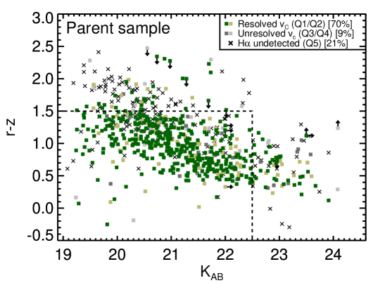
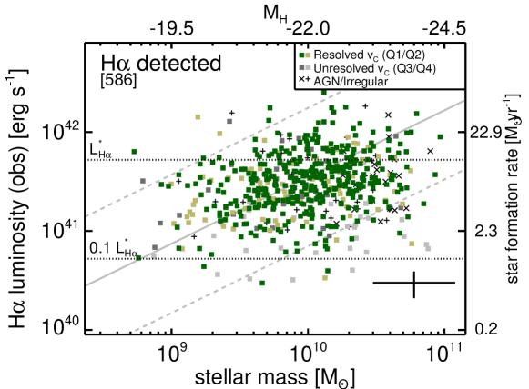
Figure 1: Left: The $r-z$ colour versus observed $K_{{\rm AB}}$ magnitude for the parent KROSS sample. The square symbols represent the 586 H$\alpha$ detected sources used for dynamical analyses in this work; with green symbols representing sources which have spatially-resolved velocity measurements (dark/light corresponds to quality 1/quality 2 [Q1/Q2]; see Section 3.4) and grey symbols representing sources that have spatially-unresolved velocity measurements (dark/light corresponds to quality 3/quality 4 [Q3/Q4]). The dashed lines show the selection criteria for the highest priority targets. Right: Observed H$\alpha$ luminosity versus stellar mass (scaled from $M_{H}$; top axis; Section 2.2) for the H$\alpha$ detected targets. The symbols are coloured as in the left panel. Systematic error bars are shown in the bottom right. The solid line shows the “main sequence” of star forming galaxies at $z$=0.85 (Speagle et al. 2014; see Section 2.3) and the grey dashed lines are a factor of five above and below this. The dotted lines show 0.1$\times$ and 1$\times$$L^{\star}_{\rm H\alpha}$ for this redshift (Sobral et al. 2015). The targets have a median star-formation rate of 7 M_⊙ yr^-1 and are representative of typical star-forming galaxies.

KROSS is an IFS survey of 795 $z$$=$0.6–1.0 typical star-forming galaxies designed to spatially-resolve the H$\alpha$ emission-line kinematics. The targets were selected from four extragalactic deep fields that are covered by a wide range of archival multi-wavelength photometric and spectroscopic data: (1) Extended Chandra Deep Field South (E-CDFS; see Giacconi et al. 2001; Lehmer et al. 2005); (2) Cosmological Evolution Survey (COSMOS; see Scoville et al. 2007); (3) UKIDSS Ultra-Deep Survey (UDS; see Lawrence et al. 2007) and (4) SA22 field (see Steidel et al. 1998 and references there-in). Most targets were selected using new or archival spectroscopic redshifts; however, $\approx$25 per cent of the sample were selected as $z=0.84$ narrow-band H$\alpha$ emitters from the HiZELS and CF-HiZELS surveys (Sobral et al. 2013a; Sobral et al. 2015). Targets were selected so that the H$\alpha$ emission line is redshifted into the $J$-band, with a higher priority given to targets where the wavelength range of the redshifted emission line is free of bright sky lines. The median redshift of the sample is $z$$=$0.85${}_{-0.04}^{+0.11}$. The details of the redshift catalogues used for selection are provided in Stott et al. (2016).

In addition to the redshift criteria, the targets were prioritised if they have observed magnitudes of $K_{\rm AB}<22.5$, corresponding to a stellar mass limit of approximately $\log$($M_{\star}$[M_☉])$\gtrsim$9.5 (see below) and they have a ‘blue’ colour of $r-z$$<$1.5 (see Figure 1). The $r-z$ colour cut reduces the chance of observing passive galaxies and, potentially, very dusty star-forming galaxies for which it is challenging to obtain high signal-to-noise H$\alpha$ observations. However, we show how our final sample represents typical $z$$\approx$1 star-forming galaxies in Section 2.3.

2.2 Stellar masses

The KROSS targets are located in extragalactic deep fields with archival optical–infrared photometric data. Therefore it is possible to measure optical magnitudes and estimate stellar masses (see details in Stott et al. 2016). For this work, we avoid using individual stellar mass estimates from the spectral energy distributions (SEDs) due to the varying quality data across the four fields. For consistency we use interpolated absolute rest-frame $H$-band AB magnitudes ($M_{{\rm H}}$) and convert to stellar masses with a fixed mass-to-light ratio ($\Upsilon_{{\rm H}}=0.2$) following $M_{\star}=\Upsilon_{\rm H}\times 10^{-0.4\times(M_{H}-4.71)}$. This mass-to-light ratio is the median value for the sample derived using the hyperz SED-fitting code (Bolzonella et al. 2000) with a suite of spectral templates from Bruzual & Charlot (2003) and the $U$-band to IRAC 4.5$\mu$m photometry. The inner 68 per cent range is 0.3 dex around the median mass-to-light ratio which we take to be the systematic uncertainty on the stellar masses (see Figure 1). Our targets are dominated by blue galaxies (Figure 1) that are likely to have similar mass-to-light ratios; however, the implications on our angular momentum versus galaxy morphology results of the potentially systematic different mass-to-light ratios for redder versus bluer galaxies is discussed in Section 4.4.

2.3 A representative sample of star-forming galaxies

For this work we apply additional cuts to the original sample presented in Stott et al. (2016). Firstly we remove 19 sources for which there were pointing errors with the IFUs such that they have unreliable kinematic measurements. Secondly, we consider the observed magnitude range of $19<K_{{\rm AB}}<24.5$ and remove any sources which have photometry that is flagged as unreliable in $r$, $z$ or $K_{{\rm AB}}$. This leaves a final sample of 743 targets (93 per cent of the original sample). Overall 552 (74 per cent) of the final sample lie in the high priority selection criteria of $r-z<1.5$ and $K_{\rm AB}<22.5$ (see Figure 1). As expected, the H$\alpha$ detection rate is higher for these targets with 478 (87 per cent) detected for the high priority and 108 detected (57 per cent) for the lower priority targets (see Section 3.2 for detection criteria). Overall 586 targets (79 per cent) from the final sample are detected in H$\alpha$ (see Section 3.2).

In Figure 1 we plot H$\alpha$ luminosity (see Section 3.2) versus estimated stellar mass for the H$\alpha$ detected targets. The full stellar mass range of this sample is $\log(M_{\star}[M_{\odot}])$=8.7–11.0, with a median of $\log(M_{\star}[M_{\odot}])$=10.0${}_{-0.4}^{+0.4}$. The median observed H$\alpha$ luminosity is $\log(L_{{\rm H}\alpha}[{\rm ergs^{-1}}])$=41.5${}_{-0.3}^{+0.3}$, which corresponds to $\approx$0.6 $L^{\star}_{{\rm H}\alpha}$ at $z\approx 1$ (Sobral et al. 2015). Overall 79 per cent of the sample have luminosities between 0.1$L^{\star}_{{\rm H}\alpha}$ and $L^{\star}_{{\rm H}\alpha}$ (see Figure 1). The median H$\alpha$ derived star-formation rate of our sample is 7${}^{+7}_{-4}$ M_⊙ yr^-1, following Kennicutt (1998) corrected to a Chabrier initial mass function and assuming an extinction of $A_{{\rm H}\alpha}=1.73$ (the median from our SED fitting, following Wuyts et al. 2013 to convert between stellar and gas extinction; see Stott et al. 2016). The median star-formation rate of our H$\alpha$ detected sample is consistent with the average star-formation and scatter of “main sequence” galaxies for the median mass and median redshift ($z=0.85$) of our targets from various works; e.g., SFR_MS=$5^{+5}_{-2.5}$ M_⊙ yr^-1 from Schreiber et al. (2015) or SFR_MS=$8^{+5}_{-3}$ M_⊙ yr^-1 from Speagle et al. (2014), where we have converted to a Chabrier IMF in both cases (see Figure 1).

For the following analyses of this paper we only discuss the $\approx$80 per cent of the final sample that are H$\alpha$ detected sources. However, based on the above, we conclude that the star-formation rates of this sample are representative of the “main sequence” of star-forming galaxies and these sources can be considered to be typical star-forming galaxies at this redshift (also see Stott et al. 2016 and Magdis et al. 2016).

2.4 KMOS observations

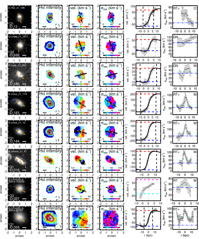
Figure 2: Example spatially-resolved galaxies from the KROSS sample (with examples from each field studied and covering the range in data quality). From left to right: (1) broad-band image (3-colour when available for the HST covered targets) where the dashed orange line represents PA_im (IDs and quality flags are also shown); (2) H$\alpha$ intensity map where the overlaid contours show the distribution of continuum emission and the dashed circle represents the seeing FWHM; (3) observed H$\alpha$ velocity map where the solid black line represents PA_vel and the dashed orange line represents PA_im; (4) observed H$\alpha$ velocity dispersion map ($\sigma_{{\rm obs}}$) where the lines are as in panel 3; (5) velocity profiles extracted along PA_vel where the solid curve is the disk model and the vertical dashed lines are the radii at which the rotational velocities are measured (average of horizontal dashed lines); however, for quality 3 sources the velocities are estimated from the galaxy-integrated spectra (e.g., ID 337); (6) observed velocity dispersion profile extracted along PA_vel where the horizontal dotted line is at $\sigma_{{\rm 0,obs}}$, the dot-dashed line is at $\sigma_{{\rm 0}}$. The solid horizontal lines in panels 1 and 2 represent 5 kpc in extent. The equivalent figures for all spatially-resolved targets are available online (see Appendix A).

The KROSS observations were taken using the KMOS instrument on ESO/VLT. KMOS consists of 24 integral field units (IFUs) that can be placed within a 7.2 arcminute diameter field. Each IFU is 2.8 $\times$ 2.8 arcsec in size with 0.2 arcsec pixels. The observation were taken during ESO periods P92–P95 using Guaranteed Time Observations (Programme IDs: 092.B-0538; 093.B-0106; 094.B-0061; 095.B-0035). The sample is also supplemented with science verification data (Programme ID: 60.A-9460; see Sobral et al. 2013b; Stott et al. 2014). The median $J$-band seeing for the observations was 0.7 arcsec, with 92 per cent of the targets observed during seeing that was $<$1 arcsec. The individual seeing measurements are taken into account during the analyses. All observations were taken using the $YJ$ band with a typical spectral resolution of $R$=$\lambda/\Delta\lambda$=3400. We correct for the instrumental resolution in the analyses presented here. Individual frames have exposure times of 600s and a chop to sky was performed every two science frames. Most targets were observed with 9 ks on source, with a minimum of 1.8 ks and a maximum of 11.4 ks (see Stott et al. 2016).

The data were reduced using the standard esorex/spark pipeline (Davies et al. 2013). However, each AB pair was reduced individually, with additional sky subtraction being performed on each pair using residual sky spectra obtained from dedicated sky IFUs. These AB pairs were flux calibrated using corresponding observations of standard stars that were observed during the same night as the science data. The individual AB pairs were then stacked using a clipped average and re-sampled onto a pixel scale of 0.1  arcsec (Stott et al. 2016). These cubes were used to create the spectra, the line and continuum images and the H$\alpha$ intensity, velocity and velocity dispersion maps used in the analyses presented here (see Section 3.2).

2.5 Comparison samples

For our specific angular momentum measurements, we focus on a comparison to the local galaxy sample presented in Romanowsky & Fall (2012) (see Section 4.3). This comprehensive study contains kinematic measurements (primarily from longslit data) for $\approx$100 nearby bright galaxies including a range of morphologies from early-type galaxies to disk-dominated spiral galaxies. They calibrate global relationships between observed velocities, radii and intrinsic specific angular momentum. Therefore, we use this study to guide our analysis techniques, using velocities obtained at the same physical radii as in their study (i.e., 2$\times$$R_{1/2}$) and the same global relationships to estimate specific angular momentum using velocity, inclination angle and radii measurements (see Section 3). When quoting $z$=0 disk angular momentum we use the raw values of disk radii, velocity and inclination angle provided by Romanowsky & Fall (2012) for the spiral galaxies and apply consistent methods to that adopted for our sample (Section 4.3). In the absence of an alternative, we use the angular momentum measurements for the early-type galaxies directly quoted by Romanowsky & Fall (2012). We apply the colour-dependant corrections to the Romanowsky & Fall (2012) total stellar masses using ($B-V$)₀ colours from Paturel et al. (2003) and Equation 1 of Fall & Romanowsky (2013). We note that our data traces angular momentum using H$\alpha$ emission which may result in $\approx$0.1 dex larger angular momentum compared to stellar angular momentum, based on low-redshift measurements (e.g., Cortese et al. 2014, 2016). We discuss this further in Section 4.3.

Cortese et al. (2016) recently presented IFS results on the angular momentum of $\approx$500 $z<0.1$ galaxies with $\log(M_{\star}[{\rm M}_{\odot}])>8$ from the sami survey (Bryant et al. 2015). Although this sample is larger than Romanowsky & Fall (2012), their specific angular momentum measurements are constructed using a very different method (following Emsellem et al. 2007) and are restricted by limitations such as only measuring the angular momentum within a small radii of $R_{1/2}$ and removing small galaxies from their sample. Therefore, for this study, we use their sample for a qualitative comparison only (Section 4.3).

In Section 4.2 we compare our rotation velocity-mass relationship to the relationship presented for 189 $z<0.1$ disk galaxies in Reyes et al. (2011). The Reyes et al. (2011) sample is ideal as it also uses H$\alpha$ emission as a tracer of rotational velocity and covers the same stellar mass range as our sample (see Tiley et al. 2016 for further discussion on low-redshift samples).

3 Analysis

In this study we investigate the rotational velocities and specific angular momentum ($j_{s}$) of H$\alpha$ detected galaxies. Towards this we make measurements of the galaxy sizes, intrinsic velocity dispersions and inclination-corrected rotational velocities. We combine archival high spatial resolution broad-band imaging, which trace the stellar light profile (Section 3.1), with H$\alpha$ velocity and velocity dispersion maps derived from our KMOS IFU data, which trace the galaxy kinematics (Section 3.2). These analyses build upon the initial kinematic analyses of the KROSS data, which does not include the broad-band imaging analyses, presented in Stott et al. (2016) who investigated disk properties and gas and dark matter mass fractions and in Tiley et al. (2016) who investigated the Tully-Fisher relationship. For all of the 586 H$\alpha$ detected targets the raw and derived quantities, along with all of the necessary flags described in the following sub sections, are tabulated in electronic format (see Appendix A).

3.1 Broad-band imaging and alignment of data cubes

To make measurements of the half-light radii ($R_{1/2}$), morphological axes (PA_im) and inclination angles ($\theta_{{\rm im}}$) we make use of the highest spatial resolution broad-band imaging available. With the aim of obtaining the best characterisation of the stellar light profile for each target we prefer to use near infrared $H$- or $K$- band images; however, we use optical images obtained using HST in preference to ground-based near infrared images, when applicable, due to the $\gtrsim$5$\times$ better spatial resolution. Overall 46 per cent of the sample have HST coverage, whilst the remainder are covered by high-quality ground-based observations (details below). We perform various tests to assess the reliability of our measurements obtained using these different data sets. Example images of our targets are shown in Figure 2.

3.1.1 Broad-band images

All of our targets in E-CDFS and COSMOS, and a subset of the targets in UDS have been observed with HST observations. These data come from four separate surveys (1) CANDELS (Grogin et al. 2011; Koekemoer et al. 2011); (2) ACS COSMOS (Leauthaud et al. 2007); (3) GEMS (Rix et al. 2004) and (4) observations under HST proposal ID 9075 (see Amanullah et al. 2010). Overall, WFC3-$H$-band observations are available for 36 per cent of the HST observed targets (CANDELS fields) with a PSF of FWHM$\approx$0.2 arcsec. For the remainder, we use the longest wavelength data available, that is, ACS-$I$ for 57 per cent and ACS-$z^{\prime}$ for 7 per cent, which have a PSF of FWHM$\approx$0.1 arcsec.

Due to the different rest-frame wavelengths being observed for the different sets of images we test for systematic effects. We measure the key properties of $R_{1/2}$, $\theta_{{\rm im}}$ and PA_im (see Section 3.1.2) using both the $H$-band and $I$-band images for the 128 targets where these are both available. We find that the median ratios and standard deviation between the two measurements to be: $R_{1/2,I}/R_{1/2,H}=1.1\pm 0.2$; $\theta_{{\rm im},I}/\theta_{{\rm im,H}}=1.0\pm 0.2$ and PA_im,I/PA${}_{{\rm im,H}}=1.0\pm 0.1$. This test indicates that our position angle and inclination angle measurements are not systematically affected by the different bands. However, the observed $I$-band sizes measurements are systematically higher than the observed $H$-band size measurements by $\approx$10 per cent. This is consistent with the HST-based results of van der Wel et al. (2014) (using their Equation 1) who find that $z\approx 0.9$, $\log(M_{\star}[M_{\odot}])$=10 galaxies are a factor of $\approx$1.2$\pm$0.2 larger in the observed $I$-band compared to in the observed $H$-band, where the quoted range covers the results for the stellar mass range $\log(M_{\star}[M_{\odot}])=$9–11. We apply a 10 per cent correction to account for this effect in Section 3.1.2.

For the UDS targets, which are not covered by HST observations, we make use of Data Release 8 $K$-band observations taken with the UKIRT telescope as part of the UKIDSS survey (Lawrence et al. 2007). The stacked image has a PSF of FWHM=0.65 arcsec. Finally, for the SA22 targets we make use of the $K$-band imaging from the UKIDSS Deep Extragalactic Survey of this field (Lawrence et al. 2007). These images have a typical PSF of FWHM=0.85 arcsec. We deconvolved the size measurements to account for the seeing in each field (Section 3.1.2).

To assess the impact of the poorer spatial resolution of the ground based images compared to the HST images we convolve the HST $H$-band images from our sample to a Gaussian PSF of: (1) FWHM=0.65 arcsec (i.e., the UDS PSF) and (2) FWHM=0.85 arcsec (i.e., the SA22 PSF), before making the measurements of radius, positional angle and inclination angle (described below). On average, position angles are unaffected by the convolution in both cases, with a median ratio of PA_im,conv/PA${}_{{\rm im,HST}}=1.0$; however an introduced 1$\sigma$ scatter of 10 per cent and 20 per cent for the UDS PSF and SA22 PSF, respectively. Similarly the inclination angles are unaffected, on average, by the convolution, with $\theta_{{\rm im,conv}}/\theta_{{\rm im,HST}}=1.0$, but with an introduced 1$\sigma$ scatter of 15 per cent and 20 per cent, respectively. We include these percentage scatters as uncertainties on the measured inclination angles from the ground based images. Following the methods described in Section 3.1.2 we find a small systematic fractional increase the measured half-light radii after the convolution of 5%; however, this is negligible compared to the introduced 1$\sigma$ scatter of 25 per cent and 35 per cent. We include these percentage scatters as uncertainties on the measured half-light radii from the ground based images.

3.1.2 Position angles, inclination angles and sizes

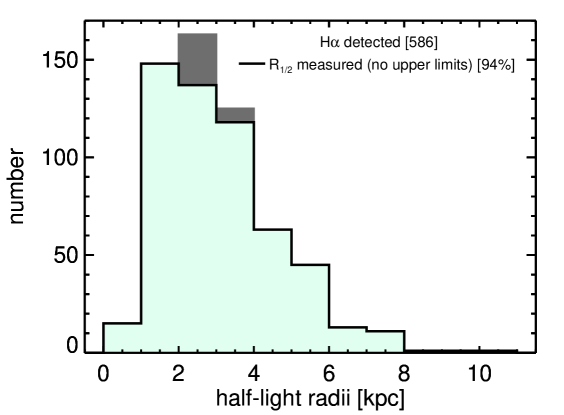
Figure 3: Distribution of continuum half-light radii, including upper limits, for the H$\alpha$ detected targets. The distribution for the 94 per cent of targets with measured radii (i.e., excluding upper limits) is shown as the overlaid filled green histogram. The majority of our galaxies have spatially-resolved radii measurements.

We aim to apply a uniform analysis across all targets irrespective of the varying spatial resolution of the supporting broad-band imaging. However, we are able to make use of more complex analyses on the HST-CANDELS subset of targets for a baseline for comparison (van der Wel et al. 2012). Furthermore, we define various quality flags, detailed below, to keep track of the quality and assumptions of the anaylses that were applied for individual targets. “Quality 1” targets are H$\alpha$ detected targets that are spatially-resolved in the IFU data (Section 3.2) and have inclination angles and position angles measured directly from the broad-band imaging (detailed below).

To obtain morphological position angles (PA_im) and axis ratios of our targets we initially fit the broad-band images with a two-dimensional Gaussian model. To obtain inclination angles ($\theta_{{\rm im}}$) we correct the axis ratios ($b/a$) for the PSF of each image and then convert these into inclination angles by assuming,

$$\cos^{2}\theta_{{\rm im}}=\frac{(b/a)^{2}-q_{0}^{2}}{1-q_{0}^{2}},$$ (1)

where $q_{0}$ is the intrinsic axial ratio of an edge-on galaxy (e.g., Tully & Fisher 1977) and could have a wide range of values $\approx$0.1–0.65 (e.g., Weijmans et al. 2014; see discussion in Law et al. 2012). We use $q_{0}=0.2$, which is applicable for thick disks; however, as a guide, a factor of two change in $q_{0}$ results in a $<$7 per cent change in the inclination-corrected velocities for our median axis ratio. To be very conservative in our uncertainties arising from the assumed intrinsic geometry we set the uncertainties of the inclination angles to be a minimum of 20%.

We compared our morphological position angles and inclination angles to those presented in van der Wel et al. (2012) for the 142 targets that overlap with the parent KROSS sample (see Section 2.3). van der Wel et al. (2012) fit Sérsic models to the HST near-infrared images using galfit that incorporates PSF modelling. Excluding the 4 targets flagged as poor fits by van der Wel et al. (2012), we find excellent agreement between the galfit results and those derived using our method. The median difference in the inclination angles are $\Delta\theta_{{\rm im}}=0.4^{+5}_{-3}$ degrees. For the position angles the median difference is $|\Delta$PA${}_{{\rm im}}|=1.8$ degrees with 84 per cent agreeing within 6 degrees. This demonstrates that there are no systematic differences between the two methods. We also compared our inclination angles for 152 of our COSMOS targets with $I$-band images to those derived using the axis ratios presented in Tasca et al. (2009) for the same sources. Again, we find excellent agreement with $\Delta\theta_{{\rm im}}=-0.4^{+7}_{-4}$ degrees. We also note that we find good agreement between the morphological position angles and kinematic position angles for both the HST targets and ground-based targets (see Section 3.3.2), which provides further confidence on our derived values. Motivated by the small scatter of the above comparisons, we enforce an additional error of 5^o on all of the inclination angle measurements. The ground based measurements have an additional uncertainty of 15 per cent and 20 per cent respectively for UDS and SA22 due to the effects of the poorer resolution for these targets (see details in Section 3.1.1).

For 7 per cent of the H$\alpha$ detected targets we are unable to measure the inclination angles from the imaging due to poor spatial resolution. For these sources we assume the median axis ratio of the targets with spatially-resolved HST images ($b/a$)$=$0.62${}_{-0.22}^{+0.20}$ (i.e., $\theta_{{\rm im}}$=53${}_{-18}^{+17}$ degrees). This median axis ratio is in agreement with the results of Law et al. (2012) who use the rest-frame HST optical images for $z\approx$1.5–3.6 star-forming galaxies and find a peak axis ratio of ($b/a$)$\approx$0.6. This assumed inclination value for these 7 per cent of our H$\alpha$ detected targets results in a correction factor of 1.2${}^{+0.5}_{-0.2}$ to the observed velocities. These targets are flagged as “quality 2” sources.

To measure the half-light radii of the broad-band images we adopted a non-parametric approach. We measured the fluxes in increasingly large elliptical apertures centred on the continuum centres that have position angles and axis ratios as derived above. We measure $R_{1/2}$ as the PSF-deconvolved semi-major axis of the aperture which contained half of the total flux. For the targets where the images are in the $I$ or $z^{\prime}$ band we apply a systematic correction of a factor of 1.1 to account for the colour gradients (see Section 3.1.1). To test our technique, we compared to the galfit Sérsic fits to the same HST data of van der Wel et al. (2012) for the targets covered by both studies. We find that the median offset between the two measurements to be $\Delta R_{1/2}/R_{{\rm 1/2,GALFIT}}=-0.01$ with a 30 per cent 1$\sigma$ scatter. Reassuringly we also did not see any trend in the offset between these too measurements as a function of magnitude. This indicates that the two methods are in general agreement; however, we assume a minimum error of 30 per cent (due to the method) on all of our half-light radii measurements. The ground based measurements have an additional uncertainty of 25 per cent and 35 per cent respectively for UDS and SA22 due to the effects of the poorer spatial resolution of the broad-band imaging for these targets (see details in Section 3.1.1).

For 84 of the H$\alpha$ detected targets we were unable to use the imaging to determine $R_{1/2}$ from the broad-band imaging; however, we were able to use the turn-over radius from the dynamical models to estimate $R_{1/2}$, calibrated using the imaging radii for the resolved sources (see Section 3.3.3). We highlight these sources as “quality 2” sources (see Figure 1). For a further 33 targets (only 6 per cent of the H$\alpha$ detected targets), where we were not able to extract radii from the IFU data or the broad band imaging , we assume conservative upper limits on the half-light radii of 1.8$\times$$\sigma_{PSF}$.

A histogram of the half-light radii for the 586 H$\alpha$ detected targets is shown in Figure 3. The median half-light radii is 2.9${}^{+1.8}_{-1.5}$ kpc (excluding upper limits). Including the upper limit targets with zero radii or their maximum possible radii, results in a median of 2.7 kpc or 2.8 kpc, respectively. The median half-light radii for the H$\alpha$ undetected targets is 2.7${}^{+1.5}_{-1.1}$ kpc and therefore, these are not significantly different in size to those that were detected.

3.1.3 Data cube alignment

To align our KMOS data cubes to the broad-band imaging we made use of continuum measurements in the data cubes. We produced continuum images by taking a median in the spectral direction, avoiding spectral pixels in the vicinity of emission lines and applying 2-$\sigma$ clipping, to avoid regions with strong sky line residuals. We identify the continuum centroids for 85 per cent of the H$\alpha$ detected targets. Due to faint continuum emission for 15 per cent of the targets we were required to obtain centroids from images including the continuum and emission lines. Examples of continuum images are shown as contours in Figure 2. These continuum centres were then used to align the data cubes to the centres of the archival broad-band images.

3.2 Emission line fitting and maps

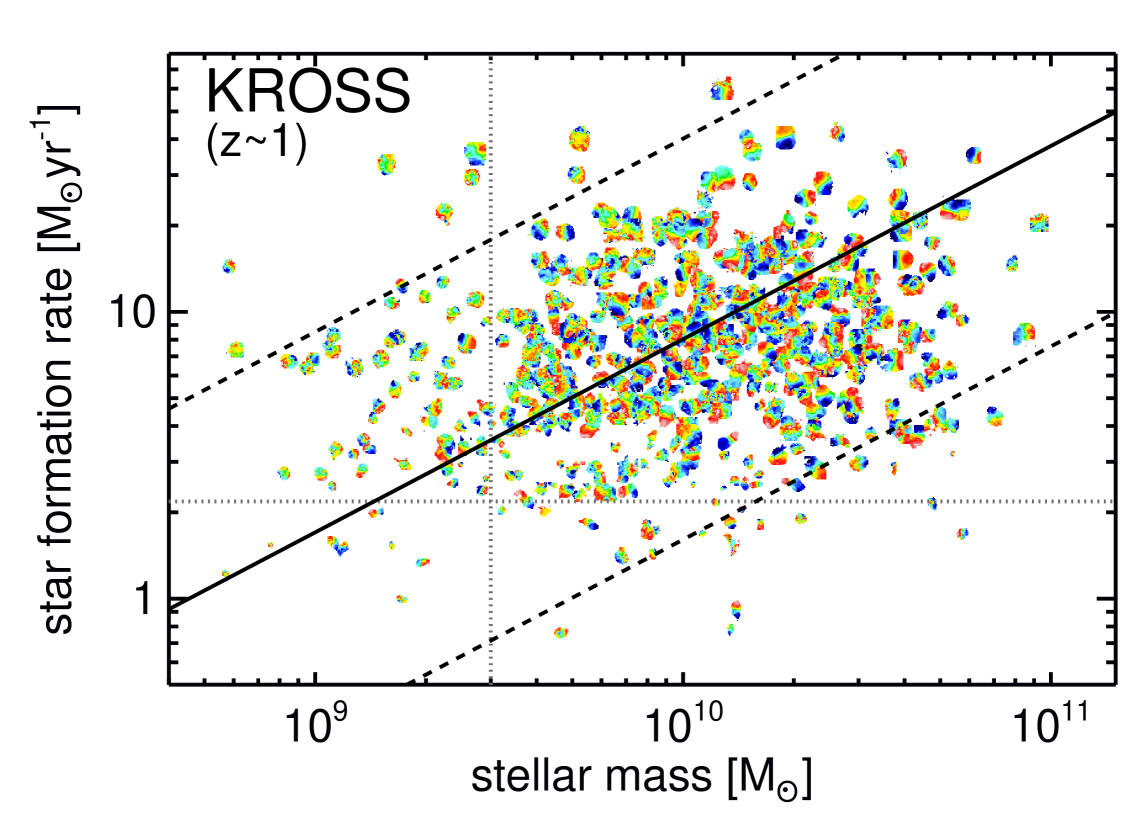
Figure 4: Velocity maps for all of our 552 spatially-resolved targets. Each map is positioned at the corresponding position in the star-formation rate versus stellar mass plane as described by the axes. The solid line shows the “main sequence” of star-forming galaxies at $z$=0.85 from Speagle et al. (2014) and the dashed lines are a factor of five above and below this. The vertical dotted line corresponds to our selection criteria for high priority targets (see Figure 1 and Section 2.1). The horizontal dotted line represents the 5th percentile of the star-formation rates of the spatially-resolved targets.

In this sub-section we describe the various kinematic measurements we make using our IFU data. These include both galaxy-integrated and spatially-resolved measurements (e.g., rotation velocities, intrinsic velocity dispersions and kinematic major axes). We produce both galaxy-integrated spectra and two dimensional intensity, velocity and velocity dispersion maps. In the following sub-sections we describe how we fit the H$\alpha$ and [N ii]6548,6583 emission-line profiles, produce the spectra and maps and make the kinematic measurements. Example maps are shown in Figure 2 and all velocity maps for the 552 targets that are spatially-resolved sources in the IFU data are shown in Figure 4.

3.2.1 Emission line fitting

We fit the H$\alpha$ and [N ii]6548,6583 emission-line profiles observed in both galaxy-integrated spectra and spectra extracted from spatial bins to derive emission-line fluxes, line widths and centroids. These fits were performed using a $\chi^{2}$ minimisation method, where we weighted against the wavelengths of the brightest sky lines (Rousselot et al. 2000). The emission-line profiles were characterised as single Gaussian components with a linear local continuum. The continuum regions were defined to be two small line-free wavelength regions each side of the emission lines being fitted. To reduce the degeneracy between parameters, we couple the [N ii]6548,6583 doublet and H$\alpha$ emission-line profiles with a fixed wavelength separation using the rest-frame vacuum wavelengths of 6549.86Å, 6564.61Å  and 6585.27Å. We also require that all three emission lines have the same line width and we fix the flux ratio of the [N ii] doublet to be 3.06 (Osterbrock & Ferland 2006). These constraints leave the intensity of the H$\alpha$ and the [N ii] doublet free to vary, along with the overall centroid, line width and continuum. The emission-line widths are corrected for the instrumental dispersion, which is measured from unblended sky lines near the observed wavelength of the H$\alpha$ emission.

3.2.2 Galaxy-integrated spectra and velocity maps

Galaxy-integrated spectra were created from the cubes by summing the spectra from the spatial pixels that fall within a circular aperture of diameter 1.2 arcsec centered on the continuum centroid. We then fit the H$\alpha$ and [N ii] emission-line profiles using the methods described above to derive: (1) the “systemic” redshift of each target; (2) the observed velocity dispersion $\sigma_{{\rm tot}}$ and (3) the H$\alpha$ flux. Sources were classed as detected if the signal-to-noise ratio, averaged over 2$\times$ the derived velocity FWHM of the H$\alpha$ line, exceeded three. The emission-line profiles and the fits for all 586 targets are available online (see Appendix A). The 1.2 arcsec aperture was chosen as a compromise between maximising the flux and signal-to-noise ratios. We estimate two methods for an aperture correction to the measured fluxes and hence to obtain galaxy-integrated H$\alpha$ luminosities. First, we use the H$\alpha$ fluxes (i.e., with [N ii] removed) presented in Sobral et al. (2013a) for the HiZELS sources for the 112 of our H$\alpha$ detected targets that overlap between the surveys. We obtain a median aperture correction of 1.7. Secondly, we re-measure the fluxes again from our IFU data but using an aperture with a diameter of 2.4 arcsec. Using the sources which are detected in both apertures we obtain a median aperture correction of 1.3. Within the uncertainties we did not find a significant correlation between aperture correction and galaxy size. Therefore, we apply a fixed aperture correction factor of 1.5 to the measured H$\alpha$ fluxes and a 30 per cent error to reflect the uncertainty on this value.

The H$\alpha$ intensity, velocity and velocity dispersion maps were first produced by Stott et al. (2016). These were created by fitting the H$\alpha$ and [N ii] emission lines at each pixel following the procedure described above and then individual velocities are calculated with respect to the galaxy-integrated ‘systemic’ redshifts. If an individual pixel did not result in a detected line with a signal-to-noise ratio of $>$5, the spatial binning was performed until this criteria was met (up to a maximum spatial of 0.7$\times$0.7 arcsec; i.e., the typical seeing of the observations). For this work, these maps are further masked by visual inspection, identifying clearly bad fits due to sky lines or defects. Overall 552 (94 per cent) of the H$\alpha$ detected sources show spatially-resolved emission (see Stott et al. 2016). We assign all of the unresolved sources a flag of “quality 4”. Example H$\alpha$ intensity, velocity and velocity dispersion maps are provided in Figure 2 and all velocity maps are shown in a star-formation rate versus stellar mass plane in Figure 4.

3.3 Spatially-resolved kinematic measurements

3.3.1 Kinematic major axes

To identify the kinematic major axes for all of the targets in our dynamical sample we make use of the H$\alpha$ velocity maps. We rotated the velocity maps around the continuum centroids (see Section 3.1.3) in 1 degree steps, extracting the velocity profile in 1.5 arcsec width “slits” and calculating the maximum velocity gradient along the slit. The position angle with the greatest velocity gradient was identified as being the major kinematic axis (PA_vel).

3.3.2 Morphological versus kinematic major axes

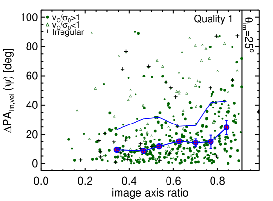
Figure 5: The difference between the photometric and kinematic position angles ($\Psi$) as a function of broad-band image axis ratio. The larger symbols represent sources covered by broad-band HST imaging. The largest data points with the error bars show the running median for the rotationally-dominated systems and the thin curve shows the running 84th percentile. For the rotationally-dominated sources the median misalignment if 13^∘. The good agreement between the positional angles observed for targets both with and without HST imaging places confidence on our measurements (see Section 3.3.2).

Here we compare the derived kinematics major axes, PA_vel, with the morphological positional angles, PA_im for our targets. Following Wisnioski et al. (2015) (c.f. Franx et al. 1991) we define the “misalignment” between the two position angles as,

$$\sin\Psi=|\sin\left({\rm PA}_{{\rm im}}-{\rm PA}_{{\rm vel}}\right)|,$$ (2)

where $\Psi$ is defined as being between 0^∘ and 90^∘. In Figure 5 we show $\Psi$ as a function of image axis ratio for the sources where we have measured the kinematic position angles, morphological position angles and axis ratios (i.e., “quality 1” sources). As expected, the dispersion-dominated systems with a low rotation velocity, $v_{C}$, to intrinsic velocity dispersion, $\sigma_{0}$, ratio (i.e., $v_{C}/\sigma_{0}<1$; see Section 4.1) have larger misalignments due to a lack of a well defined kinematic axis. For the rotationally-dominated sources, the median misalignment is 13^∘ and 81 per cent have a misalignment of $\lesssim$30^∘. These values are comparable to those found by using IFU data for high-$z$ galaxies, all with complementary HST imaging (Wisnioski et al. 2015; Contini et al. 2016). Encouragingly, our misalignment results are similar when only considering our targets without HST imaging, with a median misalignment of 15^∘ and 82 per cent having a misalignment of $\lesssim$30^∘. This provides confidence in our analyses based on the ground-based images.

3.3.3 Velocity profiles and rotational velocities

We extract one-dimensional velocity profiles [$v(r)$] along the major kinematic axes. To achieve this, we extract the median velocity in 0.7 arcsec “slits” along the velocity maps, centred on the continuum centroids (see Section 3.1.3). Examples can be seen in Figure 2 where the errors bars represent the scatter across the slit.

To reduce the effect of noise in the outer regions of the velocity profiles we extrapolate through the data points by fitting an exponential disk model (see Freeman 1970) to the velocity profiles in the form of,

$$v(r)^{2}=\frac{r^{2}\pi G\mu_{0}}{R_{D}}\left(I_{0}K_{0}-I_{1}K_{1}\right)+v_{{\rm off}},$$ (3)

where $r$ is the radial distance, $\mu_{0}$ is the peak mass surface density, $R_{D}$ is the disk radii, $v_{{\rm off}}$ is the velocity at $r=0$ and $I_{n}K_{n}$ are the Bessel functions evaluated at $0.5r/R_{D}$. During the fitting we also allow the radial centre to vary by 0.2 arcsec (i.e., the KMOS pixel scale). The velocity offset, $v_{{\rm off}}$, is applied to the velocity profiles before making measurements of dynamical velocities.

The primary function of the model velocity profiles is to extract velocities by interpolating through the data points and not to derive physical quantities; however, in 13% of the cases we are required to extrapolate the model beyond the data (see below). Focusing on the “quality 1” sources with HST images (i.e., those with the best constraints on the half-light radii from the broad-band imaging), we derive a median ratio of $R_{1/2}$/$R_{D}$=0.8${}_{-0.4}^{+0.5}$. This is consistent with our predictions for an intrinsic ratio of $R_{1/2}$/$R_{D}$=1.68 that has been beam-smeared during our $\approx$0.7^′′ KMOS observations (Johnson et al. in prep.; see details below). We apply this median ratio to the derived $R_{D}$ values to estimate the half-light radii for the “quality 2” sources that do not have spatially-resolved broad-band imaging data and hence that lack direct $R_{1/2}$ measurements (Section 3.1.1). Due to the uncertainty in this estimate we impose an uncertainty of 60 per cent. We note that we obtain consistent velocity measurements (see below) if we apply the commonly adopted arctan model (Courteau 1997; adopted for KROSS in Stott et al. 2016) instead of the exponential disk model, with a median percentage difference of $(v_{C,{\rm arctan}}-v_{C,{\rm disk}})/v_{C,{\rm disk}}=0.5_{-3}^{+9}$ per cent.

For consistency and to facilitate a fair comparison to our low-redshift comparison samples (see Section 2.5) we make measurements of the rotational velocities at the same physical radii for all targets. We make measurements at two different radii of 1.3 $R_{1/2}$ and 2 $R_{1/2}$. These correspond to $\approx$2.2$R_{D}$ and $\approx$3.4$R_{D}$, respectively, for an exponential disk. The first of these, we call $v_{2.2}$, is commonly adopted in the literature as it measures the velocity at the “peak” of the rotation curve for an exponential disk (e.g., Miller et al. 2011; Pelliccia et al. 2016) and we include these values for reference for interested parties. The second of these, which we call $v_{C}$, was chosen for use in our angular momentum measurement as it was shown by Romanowsky & Fall (2012) (our main comparison sample; Section 2.5) to be a reliable rotational velocity measurement across a wide range of galaxy morphologies. Furthermore, reaching large radii of $\gtrsim$ 3$R_{D}$ can be crucial for measuring the majority of the total angular momentum (e.g., Obreschkow et al. 2015). We note that this measurement also roughly corresponds to another commonly adopted value, $v_{80}$, which is the velocity measured at a radii containing 80 per cent of the light for an exponential disk (i.e. at 3.03 $R_{D}$; e.g., Pizagno et al. 2007; Reyes et al. 2011; Tiley et al. 2016).

To make the velocity measurements, we first convolve the $R_{1/2}$ values with the PSF of the individual KMOS observations and then read off the velocity at the defined radii from the model velocity profiles (see Figure 2). The observed velocities quoted, $v_{\rm obs}$, are half the difference between the velocities measured at the positive and negative side of the rotation curves. For 13 per cent of the targets in the spatially-resolved sample we are required to use the model (see above) to extrapolate to $>$0.4 arcsec beyond the data to reach (i.e., $>$2 KMOS pixels). The uncertainties on the observed velocities are obtained by varying the radii by $\pm$1 $\sigma$ and then re-measuring the velocities.

For sources where we do not have spatially-resolved IFU data (i.e., “quality 4”) or we do not have a measured half-light radii (i.e., “quality 3”) we are unable to measure the velocities at a fixed radii from the IFU data. Therefore we estimate the velocities from the widths of the galaxy-integrated emission-line profiles by applying correction factors derived from the resolved velocity measurements; i.e., the median ratios of $\sigma_{\rm tot}/v_{{\rm C,obs}}$=1.13 and $\sigma_{\rm tot}/v_{{\rm 22,obs}}$=1.26. In both cases there is 0.3 dex scatter on these ratios, which we apply as a uncertainty on these measurements.

To obtain the intrinsic velocities, $v_{2.2}$ and $v_{C}$, we apply a correction to the observed velocities for the effects of inclination angle ($\theta_{{\rm im}}$) and beam smearing following,

$$v=v_{{\rm obs}}\times\frac{\epsilon_{R,PSF}}{\sin({\theta_{{\rm im}}})},$$ (4)

where $\epsilon_{R,PSF}$ is the beam-smearing correction factor that is a function of the ratio of half-light radii to the FWHM of the KMOS PSF. These correction factors are derived in Johnson et al. (in prep.), by creating mock KMOS data (also see Burkert et al. 2016 for similar tests). A sample of $\approx$10⁵ model disk galaxies were created assuming an exponential light profile, with a distribution of sizes and stellar masses representative of the KROSS sample. The intrinsic velocity fields were constructed assuming a dark matter profile plus an exponential stellar disk, with a range of dark matter fractions motivated from the eagle simulations (Schaye et al. 2015). A range of flat intrinsic velocity dispersions, $\sigma_{0}$ were also assumed. “ Intrinsic” KMOS data cubes were constructed using the model galaxies to predict the velocity, intensity and linewidth of H$\alpha$ profiles. Each slice of these cubes was then convolved with a variety of seeing values applicable for the KROSS observations. These mock observations were then subject to the same analyses as performed on the real data. Differences between input and output values were used to derived the correction factors as a function of the ratio of half-light radii to the FWHM of the KMOS PSF. Full details will be provided in Johnson et al. in prep. For the measured $v_{C}$ values these corrections range from $\epsilon_{R,PSF}$=1.01–1.17 with a median of 1.07. We follow the same equation for $v_{2.2}$ but apply the appropriate $\epsilon_{R,PSF}$ correction factor for this radii. The uncertainties on the intrinsic velocities are calculated by combining (in quadrature) the uncertainties on the observed velocities (see above) with the variation from varying the inclination angles by $\pm$1 $\sigma$.

3.3.4 Velocity dispersion profiles and intrinsic velocity dispersions

To classify the galaxy dynamics of our sources we need to make measurements of the intrinsic velocity dispersions ($\sigma_{0}$). We extract velocity dispersion profiles [$\sigma(r)$] using the same approach as for the velocity profiles (see above) but using the observed $\sigma$ maps (see examples in Figure 2). We then measure the observed value $\sigma_{\rm 0,obs}$ in the outer regions of the $\sigma(r)$ profiles by measuring the median values from either $>$2$\times$ or $<-$2$\times$ the half-light radii (whichever is lowest). At these radii the observed velocity dispersion will only have a small contribution from the beam-smearing of the velocity field (see below). The uncertainties are taken to be the 1$\sigma$ scatter in the pixels used to calculate this median. When the extent of the data does not reach sufficient radii (or we do not have a measured half-light radii), which is the case for 52 per cent of our H$\alpha$ sample, we adopt a second approach by taking the median value of the pixels in the $\sigma$ maps. After applying the appropriate corrections (see below), these methods agree within 4 per cent (where it is possible to make both measurements) with a $\approx$50 per cent scatter. Consequently we impose an uncertainty of 50 per cent for those targets where we use the median of the velocity dispersion ($\sigma$) map to infer $\sigma_{{\rm 0,obs}}$.

For both of the approaches for measuring $\sigma_{{\rm 0,obs}}$ we obtained the intrinsic velocity dispersion, $\sigma_{\rm 0}$, by applying a systematic correction for the effects of beam-smearing based on mock KMOS data (Johnson et al. in prep; see details above). These corrections are a function of both the ratio of half-light radii to the FWHM of the KMOS PSF and the observed velocity gradient. When using the velocity dispersions extracted from the outer regions the beam-smearing corrections have a median of 0.97${}_{-0.06}^{+0.02}$ and for those extracted from the sigma maps the median correction factor is 0.8${}_{-0.3}^{+0.1}$. The intrinsic velocity dispersions of the sample will be provided and discussed in detail in Johnson et al. (in prep).

3.4 Summary of the final sample for further analyses

We detected H$\alpha$ emission in 586 of our targets (79 per cent) and we showed that these are representative of “main sequence” star-forming galaxies at $z$$\approx$1 (Section 2.3). For the following analyses, which are based on velocity measurements, we exclude the 50 sources with an inclination angle of $\theta_{{\rm im}}\leq 25^{\rm o}$ because the inclination corrections to the velocities for these sources become very high (e.g., $>$2.4 for $<$25^o and $>$10 for $<$5^o). Consequently, any small errors in the inclination angles can result in large errors in the velocity values. We remove a further 20 sources which have either an emission-line ratio of [N ii]/H$\alpha$$>$0.8 and/or a $\gtrsim$1000 km s^-1 broad line component in the H$\alpha$ emission line profiles (but not the [N ii] profile). These sources have a significant contribution to the emission lines from AGN emission and/or shocks (e.g., Kewley et al. 2013; Harrison et al. 2016). Finally, we remove a further 30 sources which show multiple emission regions in the IFU data or broad-band imaging that resulted in unphysical measurements for the rotational velocities and/or the half-light radii. This leaves a final sample of 486 targets for analyses on the rotational velocities (Section 4.2) and specific angular momentum (Section 4.3).

Of this final sample, only 33 (7 per cent) are unresolved in the IFU data (“quality 4”) and only 24 (5 per cent) are resolved in the IFU data but have only an upper limit on the half-light radii (“quality 3”; see Section 3.1.2). In both of these cases the velocity measurements are unresolved in that they are estimated from the galaxy-integrated emission-line profiles (Section 3.3.3). We note that 63 (13 per cent) are assigned “quality 2” because they have fixed (unknown) inclination angle and/or a half-light radii that is estimated from the velocity models as opposed to the broad-band imaging (see Section 3.1.2). Overall, the majority of the sources (366; i.e., 75 per cent) are assigned “quality 1” for which we have spatially-resolved IFU data and both the half-light radii and inclination angles are measured directly from the broad band imaging.

4 Results and Discussion

In the previous sections we have presented our new analyses on $\approx$600 H$\alpha$ detected galaxies from the KROSS survey. These targets are representative of typical star-forming galaxies at redshift $\approx$0.9. Using a combination of broad-band imaging and our IFU data we have measured inclination angles, half-light radii, morphological and kinematic position angles, rotational velocities and intrinsic velocity dispersions (see Appendix A for details of the tabulated version of these values). After removing highly-inclined sources and those with an AGN contribution to the line emission (Section 3.4), we are left with a sample of 486 targets for which we analyse the rotational velocities and specific angular momentum in the following subsections.

4.1 Rotational velocities and v/$\sigma_{0}$

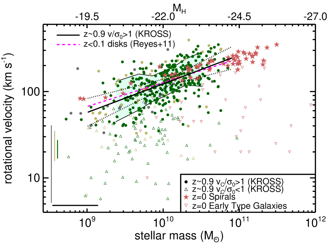
Figure 6: Rotational velocity ($v_{C}$) as a function of estimated stellar mass (scaled from $M_{H}$; top axis) for KROSS galaxies that are rotationally dominated (circles) and dispersion dominated (triangles). The symbol colours are as described in Figure 1. From left to right, the three vertical lines show the median uncertainty (in log space) for quality 3, 2 and 1 sources, respectively, and the horizontal line shows the systematic uncertainty for converting $M_{H}$ to stellar mass. The shaded region shows the running $\approx$0.2 dex (68 per cent) scatter on the velocities of the rotationally-dominated sources. We plot the best fit to these sources and the bootstrap 1$\sigma$ uncertainty (dotted lines; see Section 4.2). This is in excellent agreement with equivalent H$\alpha$ observations of local disks (Reyes et al. 2011) and stellar observations of local spiral galaxies from Romanowsky & Fall 2012. Dispersion-dominated galaxies do not follow this trend, similar to the $z$=0 early-type galaxies from Romanowsky & Fall 2012.

In Figure 6 we plot the rotational velocity ($v_{C}$) versus stellar mass for our final sample that have spatially-resolved IFU data (i.e., the 93 per cent of the targets that are classified as quality 1–3; see Section 3.4). The median rotational velocity, $v_{C}$, is $109\pm 5$ km s^-1 with the 16th and 84th percentiles of 43 km s^-1 and 189 km s^-1, respectively. The mean velocity (weighted by the fractional errors) is 117$\pm$4 km s^-1. The uncertainties on both numbers are from the width of the distribution from bootstrap re-sampling 1000 times, scattering the velocity values about their errors, and recalculating the values. These velocity measurements were made at 2$\times$$R_{1/2}$ (i.e., $\approx$3$R_{D}$; Section 3.3.3). For comparison, the median velocity with 16th and 84th percentiles at 1.3$\times$$R_{1/2}$ ($\approx$2.2$R_{D}$) is $97_{-59}^{+72}$ km s^-1. Considering these sources we find a median ratio of rotational velocity to velocity dispersion (i.e., $v_{C}/\sigma_{0}$) of $2.36\pm 0.14$ with a 16th and 84th percentiles of 0.90 and 5.04, respectively. The mean fraction, weighted by the fractional errors, is 3.05$\pm$0.18 (with errors calculated as above).

To assess if the targets are “rotationally dominated” or “dispersion dominated” we assess which of the rotational velocities or the intrinsic velocity dispersions, $\sigma_{0}$ is larger (following e.g., Weiner et al. 2006; Genzel et al. 2006). We find that 81$\pm$5 per cent are “rotationally dominated” with $v_{C}/\sigma_{0}$$>$1 (consistent with the original measurements of the KROSS sample presented in Stott et al. 2016).. The minimum and maximum values of this fraction are 52% and 90%, if the calculation is done with the individual values at their respective minimum and maximum limits, given by the error bars. These results imply that the H$\alpha$ kinematics are dominated by rotation (over dispersion) across our sample but with lower $v_{C}/\sigma_{0}$ values than the typical values of $v_{C}/\sigma_{0}$$\approx$5–10 observed in low-redshift disks (Epinat et al. 2010). This is consistent with previous work that suggest a higher fraction of the gas dynamics comes from disordered motions, with a lower fraction of “settled disks”, for increasing redshift (e.g., Puech et al. 2007; Epinat et al. 2010; Kassin et al. 2012; Wisnioski et al. 2015; see Stott et al. 2016 for a more detailed comparison to previous work).

We also create a “gold” rotationally-dominated sub-sample where we apply strictier criteria (similar to Wisnioski et al. (2015)) to isolate sources which have high quality data and look “disky” in nature. These are highlighted in relevant figures and tables (see Appendix A). This only includes quality 1 or quality 2 sources (i.e., spatially-resolved velocity measurements) and have the additional criteria of: (1) $v_{C}/\sigma_{0}>$1; (2) the kinematic and morphological position angles agree within 30^∘ and (3) the peak of the $\sigma(r)$ profile is within 0.4 arcsec (i.e., 2 pixels) of the centre of the velocity field (see Figure 2). This sub-sample represents 38% of the quality 1 and quality 2 sources; however, we caution that these criteria are subject to $\sigma$ profiles which can be noisey and this fraction has little physical meaning.

4.2 Rotational velocity versus stellar mass

The rotational velocity, $v_{C}$, versus stellar mass, $M_{\star}$, plane (Figure 6) is often referred to as the inverse of the stellar mass “Tully-Fisher relationship” (TFR; Tully & Fisher 1977; Bell & de Jong 2001). This relationship measures how quickly the stars or gas are rotating, a potential tracer for total mass (or “dynamical mass”), as a function of luminous (i.e., stellar) mass. In the context of understanding how galaxies acquire their stellar mass and rotational velocities across cosmic time, it is therefore interesting to investigate how this relationship evolves with redshift (e.g., see Portinari & Sommer-Larsen 2007 and Dutton et al. 2011). In Figure 6 we compare the $v_{C}$ versus $M_{\star}$ plane for our KROSS $z$$\approx$0.9 star-forming galaxy sample to the stellar disk velocities for $z=0$ spiral galaxies from Romanowsky & Fall (2012) and the relationship defined by Reyes et al. (2011) using spatially-resolved H$\alpha$ kinematics for $z<0.1$ disk galaxies in the same mass range as our $z$$\approx$0.9 sample (see Section 2.5). Both of these $z$$\approx$0 studies use velocities measured at $\approx$3$R_{D}$ which is consistent with our measurements.

Figure 6 shows that the rotationally-dominated KROSS galaxies have a very similar relationship between velocity and stellar mass compared to $z=0$ disks. To quantify this, we follow Reyes et al. (2011) and fit the relationship with velocity as the dependant variable in the form $\log v_{C}=b+a[\log M_{\star}-10.10]$ (see discussion in Contini et al. 2016 on the benefits of this approach). Using a least-squares fit (using mpfit; Markwardt 2009) we derive $a=0.33\pm 0.11$ and $b=2.12\pm 0.04$, where the uncertainties are the standard deviations of the results from bootstrap re-sampling the fit with replacement 1000 times, scattering the stellar masses with a 0.3 dex error each time (see Section 2.2). The Pearsons and Spearman’s Rank correlation coefficients for the KROSS sample in Figure 6 are 0.57 and 0.55, respectively. We note that if we only fit to the “gold” sub-sample as defined in Section 4.1 we obtain consistent results with $a=0.39$ and $b=2.17$).

For their $z$=0 sample sample, Reyes et al. (2011) obtained linear fit parameters of $a_{z=0}=0.278\pm 0.010$ and $b_{z=0}=2.142\pm 0.004$. Therefore, we see no evidence for an evolution in the slope or normalisation of the velocity stellar mass relationship (or stellar mass “Tully Fisher Relationship") between rotationally-dominated $z$$\approx$1 star-forming galaxies and $z$$\approx$0 disk galaxies. This lack of evolution agrees with the conclusions of most previous longslit and IFU studies of $z$$\lesssim$1 “disky” galaxies, at least for the stellar mass ranges of this work; i.e., $\log(M_{\star}$[M_⊙]$)\gtrsim 9.5$ (e.g., Conselice et al. 2005; Flores et al. 2006; Miller et al. 2011; Vergani et al. 2012; Pelliccia et al. 2016; Contini et al. 2016; Di Teodoro et al. 2016; although see Puech et al. 2010). However, we note that this relationship can change depending on the definition of “disky" or “rotationally dominated” galaxies (see Kassin et al. 2012; Tiley et al. 2016) or the chosen mass-to-light ratios, which may introduce systematic uncertainties of a factor of 3–5 (e.g., Bershady et al. 2011; Fall & Romanowsky 2013). For example, although based on the pre-liminary analysis of the KROSS sample, Tiley et al. 2016 found that applying a stricter criteria of $v/\sigma_{0}>3$ to select “disky” galaxies implies an offset of $\approx$0.4 dex towards higher stellar masses, at a fixed velocity, between $z=1$ and $z=0$. Clearly, selection effects are important for physically interpreting the evolution in the rotation velocity–mass relationship.

We do not attempt to interpret the $\approx$0.2 dex scatter in the rotation velocity-mass relationship for the KROSS sample observed in Figure 6, which is likely to be driven by a combination of observational uncertainties and physical effects such as non-rotational gas kinematics and morphological variations (e.g., Kannappan et al. 2002; Kassin et al. 2007; Puech et al. 2010; Covington et al. 2010; Miller et al. 2013; Simons et al. 2015). However, the dispersion dominated galaxies ($v_{C}/\sigma_{0}<1$) introduce significant scatter to lower velocities and do not follow a tight relationship with stellar mass. This is also the case for the $z=0$ early-type galaxies shown in Figure 6 and has previously been noted at higher redshifts as potentially being due to the rotational velocities being a poor tracer of the total dynamical mass in these sources (e.g., Kassin et al. 2007, 2012; Pelliccia et al. 2016).

It is well established that to reproduce the observed baryonic properties of galaxies (such as the stellar mass function, the mass–size relationships, and angular momentum of disks) requires feedback prescriptions that regulate the net accretion of baryons and consequently the amount of material available for star formation (e.g., Silk 1997; Abadi et al. 2003; Sommer-Larsen et al. 2003; Governato et al. 2007; Torrey et al. 2014; Crain et al. 2015). However, the TFR (i.e., Figure 6) is a poor test to constrain model feedback prescriptions. Indeed, it is possible to fit the observed TFR but with incorrect galaxy masses due to a trade off between disk size and galaxy mass (Ferrero et al. 2016; also see Guo et al. 2010). Therefore, for the remainder of this work we focus on angular momentum that incorporates observed velocities and galaxy sizes, which, along with mass and energy has been proposed as one of the fundamental properties to describe a galaxy (e.g., Fall 1983; Obreschkow & Glazebrook 2014).

4.3 Angular momentum

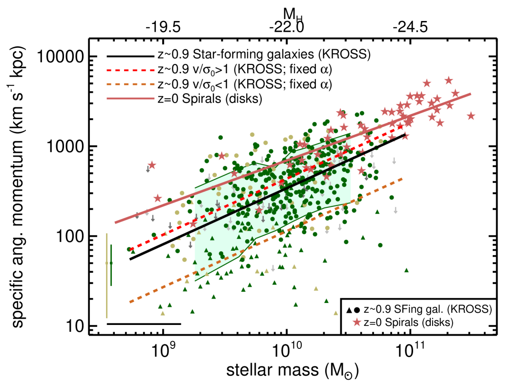
Figure 7: Specific angular momentum as a function of estimated stellar mass (scaled from $M_{H}$; top axis) for rotationally-dominated (circles) and dispersion-dominated (triangles) sources in our KROSS sample. The symbol colours are as described in Figure 1. From left to right, the two vertical lines show the median uncertainy (in log space) for quality 2 and quality 1 sources, respectively, and the horizontal line shows the systematic uncertainty for converting $M_{H}$ to stellar mass. The shaded region represents the running (68 per cent) scatter for the whole sample. The fit to the full KROSS sample reveals a relationship of $j_{s}\propto M_{\star}^{0.6\pm 0.2}$, similar to that observed for the $z$=0 spiral disks from Romanowsky & Fall 2012. The $z$=0 spiral disks have $\approx$0.2–0.3 dex more specific angular momentum for a fixed stellar mass compared to the $z$$\approx$0.9 star-forming galaxies.

In Figure 7 we plot specific angular momentum as a function of stellar mass, $M_{\star}$, for the 486 galaxies in our final sample. Specific angular momentum is defined as $j_{s}\equiv J/M_{\star}\propto R_{D}v_{C}$, where $J$ is the total angular momentum (Fall 1983). Exploring specific angular momentum is useful as it removes the implicit scaling between $J$ and mass. To enable us to uniformly apply the same methods across the sample, irrespective of data quality, we take the approximate estimator for specific angular momentum from Romanowsky & Fall (2012) (their Equation 6) that can be applied to galaxies of varying morphological types (see Romanowsky & Fall 2012 and Obreschkow & Glazebrook 2014 for potential limitations); that is,

$$j_{n}=k_{n}C_{i}v_{s}R_{1/2},$$ (5)

$v_{s}$ is the rotation velocity at 2$\times$the half-light radii ($R_{1/2}$), $C_{i}$ is the de-projection correction factor which we assume to be $1/\sin(\theta_{{\rm im}})$ (see Appendix A of Romanowsky & Fall 2012) and $k_{n}$ is a numerical coefficient that depends on the Sérsic index, $n$, of the galaxy and is approximated as,

$$k_{n}=1.15+0.029n+0.062n^{2}.$$ (6)

Following Section 3.3.3 we can use our rotational velocities in Equation 5, where $v_{C}\equiv C_{i}v_{s}$. Due to varying quality of broad band imaging (see Section 3.1), we are unable to measure $n$ for all of our galaxies. However, the 101 targets from our sample with HST imaging and Sérsic fits presented in van der Wel et al. (2012) have a median Sérsic index of $n=1.1$ and 86 per cent have $n<2$. Therefore, for the global relationships presented here (Figure 7) we assume the $n=1$ case which is applicable for exponential disks (i.e., $k_{1}=1.19$; Romanowsky & Fall 2012) and assume the specific angular momentum to be $j_{s}=j_{n=1}$. For comparison a Sérsic index of $n=2$, only results in a $\approx$20 per cent difference with $k_{2}=1.46$. We investigate the relationship between $n$ and $j_{s}$ in Section 4.4.

We parametrise the $j_{s}$–$M_{\star}$ relationship for the KROSS galaxies (Figure 7) in the form $\log j_{s}=\beta+\alpha[\log M_{\star}-10.10]$. Using a least-squares fit (using mpfit; Markwardt 2009) we obtained a slope of $\alpha$=0.6$\pm$0.2 and a normalisation of $\beta$=2.59$\pm$0.04, where the uncertainties are the standard deviations of the results from bootstrap re-sampling the fit with replacement 1000 times, scattering the stellar masses with a 0.3 dex error each time (see Section 2.2). The Pearsons and Spearman’s Rank correlation coefficients for the KROSS sample in Figure 6 are 0.46 and 0.45, respectively. We note that there is a negligible effect if we exclude or include the 11 per cent of $j_{s}$ upper limits.

We fit the specific angular momentum of the disk components of the $z$=0 spiral galaxies presented Romanowsky & Fall (2012) (following Equation 5; see Section 2.5) and obtain a slope of $\alpha_{z=0}$=0.51$\pm$0.06, consistent with the $\alpha_{z=0}$=0.6$\pm$0.1 quoted by Fall & Romanowsky (2013) for the same sample. The normalisation of $z$=0 disk relationship is $\beta_{z=0}$=2.89$\pm$0.05 and we note that we obtain a normalisation of $\beta_{z=0,\alpha}=$2.83$\pm$0.03 if we fix $\alpha$ to be the same as that we obtained for the KROSS sample.

The slope of the $j_{s}$–$M_{\star}$ relationship for the $z$=0.9 star-forming KROSS galaxies is consistent with other high and low-redshift IFU studies who found slopes of $\approx$0.6 (Cortese et al. 2016; Contini et al. 2016; Burkert et al. 2016; Swinbank et al. 2017; although see Obreschkow & Glazebrook 2014 and Cortese et al. 2016 for a discussion on how $\alpha$ might vary with bulge fraction). Our observed slope in the $j_{s}$–$M_{\star}$ relationship, tracing the angular momentum of the baryons at 2$R_{1/2}$, is close to the value of $\alpha=2/3$ predicted for dark matter haloes from both tidal torque theory and simulations (i.e., $j_{\rm halo}\propto M_{\rm halo}^{2/3}$; Shaya & Tully 1984; Heavens & Peacock 1988; Barnes & Efstathiou 1987; Catelan & Theuns 1996). If baryons and dark matter are well mixed in the proto-galaxy and the galaxies retain most of the specific angular momentum they acquired in the early phases of their formation, then $j_{\rm s}\sim j_{\rm halo}$ and the relationship would follow $j_{s}\propto M^{2/3}$ (e.g., see discussion in Romanowsky & Fall 2012; Obreschkow & Glazebrook 2014 and Burkert et al. 2016). A shallower slope than $\alpha=2/3$ implies a mass dependence on the conversion between halo angular momentum and galaxy angular momentum (e.g., Romanowsky & Fall 2012). We explore the comparison between galaxy angular momentum and dark matter haloes further in Section 4.3.1.

The normalisation of the $j_{s}$–$M_{\star}$ relationship is $\approx$0.3 dex lower in our $z$$\approx$0.9 sample compared to the $z=0$ disks (Figure 7). However, if we fit only the rotationally-dominated sources (a possible proxy for “disky” type systems in our sample), we obtain a normalisation of $\beta_{v/\sigma>1}$=2.70$\pm$0.03 (for a fixed $\alpha$=0.62). This still corresponds to a $\approx$0.2 dex offset, for a fixed mass, between the rotationally-dominated $z$$\approx$0.9 star-forming galaxies and $z$=0 disks. We note that if the H$\alpha$ measurements of $j_{s}$ are systematically higher than stellar measurements by $\approx$0.1 dex as seen at low redshift (e.g., Cortese et al. 2014, 2016) this would increase the offset observed in $j_{s}$ between $z$$\approx$0.9 and $z$=0 in Figure 7 even further. This $\approx$0.2–0.3 dex offset between $z$$\approx$0.9 star-forming galaxies and $z$=0 spiral galaxies is in contrast to what we observed in the rotation velocity–mass diagram (Figure 6) where no evolution was observed between the same samples. This implies that the primary driver of the offset between the two samples is differences in the disk sizes between the two epochs (see e.g., van der Wel et al. 2014) because $j_{s}\propto R_{D}v_{C}$. As a basis to further explore the $j_{s}$–$M_{\star}$ relationship and evolution, in the following, we compare our results to a simple model for galaxies embedded inside a dark matter halo.

4.3.1 A simple model to investigate angular momentum transfer

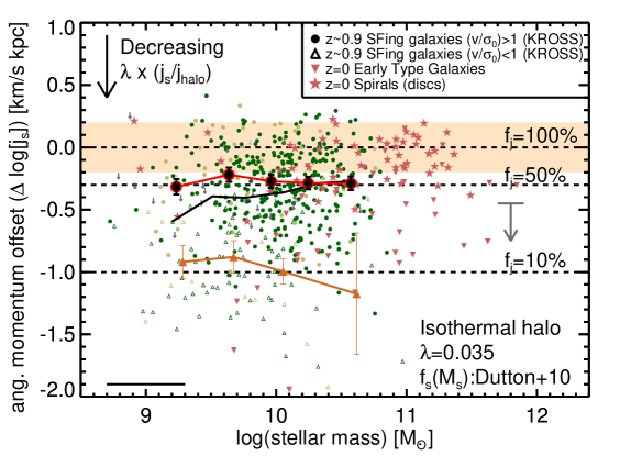
Figure 8: Specific angular momentum offset as a function of estimated stellar mass. The dashed lines represent fixed ratios of $f_{j}=j_{\rm s}/j_{\rm halo}$ following the assumptions outlined in Section 4.3.1. The shaded region represents the 0.2 dex scatter expected for the distribution of halo spins, $\lambda$. The solid red (with large symbols), black and orange solid curves represent the running median for the rotationally-dominated, total and dispersion-dominated samples respectively. The downward grey arrow represents the median systematic offset to apply to the $z$=0 early-type galaxies when using different stellar mass fractions compared to the disks (see Section 4.3.1). The rotationally-dominated galaxies have typical values of $f_{j}$$\approx$(50–60) per cent, independent of mass.

In Figure 8 we show the observed angular momentum for our KROSS sample and the $z$=0 comparison sample (see Section 2.5) compared to that predicted from a simple model of a galaxies residing inside dark mater halos. Following Section 4 of Obreschkow & Glazebrook (2014), we assume the galaxies with angular momentum, $j_{s}$, are embedded inside singular isothermal spherical cold-dark matter halos (e.g., White 1984; Mo et al. 1998) truncated at the virial radius that are characterised with spin parameter $\lambda$ (Peebles 1969; Peebles 1971) and specific angular momentum $j_{{\rm halo}}$. We explore the general case where the galaxy contains a fraction of the angular momentum of the halo, defining the ratio $f_{j}=j_{\rm s}/j_{\rm halo}$. Taking Equation 18 from Obreschkow & Glazebrook (2014) and assuming the universal baryon fraction is $f_{b}$=0.17 we obtain a predicted angular momentum of (see similar derivations in Romanowsky & Fall 2012 and Burkert et al. 2016),

$$\frac{j_{{\rm s,pred}}}{{\rm kpc\,km\,s^{-1}}}=2.95\times 10^{4}f_{j}f_{{\rm s}}^{-2/3}\lambda\left(\frac{H[z]}{H_{0}}\right)^{-1/3}\left[\frac{M_{\star}}{10^{11}M_{\odot}}\right]^{2/3}$$ (7)

where $H(z)$= $H_{0}\left(\Omega_{\lambda,0}+\Omega_{m,0}[1+z]^{3}\right)^{0.5}$ and $f_{s}$ is the stellar mass fraction relative to the initial gas mass. Following Burkert et al. (2016) (also see Romanowsky & Fall 2012) we take an initial assumption that all of the haloes have spin $\lambda$=0.035. This should be reasonable, on average, as the spin parameter is found to follow a near-log normal distribution, independent of mass, with an average around this adopted value and $\approx$0.2 dex width from both tidal torque theory and full simulations (e.g., Bett et al. 2007; Macciò et al. 2008; Zjupa & Springel 2016; also see Burkert et al. 2016 for observational constraints). Note that if $\lambda f_{j}f_{\star}^{-2/3}$ is independent of mass, Equation 7 leads to the scaling $j_{{\rm s,pred}}\propto M^{2/3}$, which is consistent with that observed in the data: $j_{s}\propto M_{\star}^{0.6\pm 0.2}$ (Figure 7). However, following Romanowsky & Fall (2012) and Burkert et al. (2016) (their Equation 6) we assume a mass dependant value of $f_{s}$ using the empirically-derived expression (obtained using abundance matching, stellar kinematics and weak lensing) for local late-type galaxies from Dutton et al. (2010) given by,

$$f_{s}=0.29\times\left(\frac{M_{\star}}{5\times 10^{10}{\rm M}_{\odot}}\right)^{0.5}\left(1+\left[\frac{M_{\star}}{5\times 10^{10}{\rm M}_{\odot}}\right]\right)^{-0.5}$$ (8)

As discussed in Section 4.4, a different expression is given by Dutton et al. (2010) for early-type galaxies.

Using these assumptions, we define the specific angular momentum offset $\Delta\log j_{\rm s}\equiv\log j_{{\rm s}}-\log j_{{\rm s,pred}}$ (setting $f_{j}$=1). We plot $\Delta\log j_{\rm s}$ as a function of stellar mass in Figure 8. Empirically, sources with lower $\Delta\log j_{\rm s}$ values have less specific angular momentum for their stellar mass than those with higher values. In the context of the model outlined above, a lower value of $\Delta\log j_{\rm s}$ corresponds to lower values of $f_{j}$, i.e., $j_{s}/j_{{\rm halo}}$, and/or the spin parameter $\lambda$. Assuming a fixed spin parameter, $\lambda$=0.035, for the rotationally-dominated $z$$\approx$0.9 KROSS galaxies, $f_{j}$ is independent of stellar mass with a bootstrap median and uncertainty of $f_{j}=0.53_{-0.03}^{+0.04}$ and a $\approx$0.3 dex scatter (Figure 8). If we only consider the “gold sample” described in Section 4.1 we obtain $f_{j}=0.64_{-0.03}^{+0.05}$, which is consistent within $\approx$2$\sigma$. For the $z$=0 spiral disks we obtain a bootstrap median and uncertainties of $f_{j}=0.77_{-0.07}^{+0.11}$ with 0.2 dex scatter, which is in agreement to the value of $f_{j}$$\approx$0.8 quoted by Fall & Romanowsky (2013) for these galaxies.

If the angular momentum of the halo and the baryons were initially well mixed with $j_{\rm baryon}\approx j_{\rm halo}$, then the results presented in Figure 8 suggest that $\approx$40–50 per cent of the initial angular momentum has been lost during the formation of $z$$\approx$0.9 star-forming “disky" galaxies. Alternatively high angular momentum gas (i.e., $>j_{\rm halo}$) entering the halo through cosmic filaments could have eventually lose angular momentum until $j_{s}\approx(0.5$–0.6)$j_{\rm halo}$ (e.g., Kimm et al. 2011; Stewart et al. 2013; Danovich et al. 2015). Whilst various idealised assumptions were required in the above analyses (see Burkert et al. 2016 for other approaches), it seems that the angular momentum of galaxies broadly follow the theoretical expectation from such a simple galaxy halo model. This is a striking result given the complexity of baryonic collapse which includes inflows, outflows, mergers and turbulence that require hydrodynamical simulations to properly model. Indeed, despite the complexity, the net angular momentum of the baryons and star-forming disks are found to be similar in models (e.g., Danovich et al. 2015; Zavala et al. 2016; Lagos et al. 2016). See Swinbank et al. 2017 for a detailed comparison between the angular momentum of $z$$\lesssim$1.5 galaxies in the EAGLE cosmological simulation (Schaye et al. 2015; Crain et al. 2015) and galaxies observed with the MUSE IFU.

We observe a small systematic offset to lower average values of specific angular momentum offset (i.e., $\Delta\log j_{\rm s}$) between the $z$$\approx$0.9 “disky" (rotation-dominated) galaxies compared to the $z$=0 disks of $\approx$0.15 dex, albeit with a large scatter (Figure 8). This offset is a reflection of the offset observed in the raw values shown in Figure 7 but now accounting for a predicted evolution of $H(z)^{-1/3}$ (see Equation 7). This small offset is qualitatively consistent with the result on $z$$\approx$0.8–2.6 star-forming galaxies in Burkert et al. (2016) when using similar assumptions (their Figure 3), although their study is dominated by higher stellar mass galaxies than ours. Furthermore, an evolution in specific angular momentum is expected for galaxy disks. Numerical models predict that redshift zero disks have more specific angular momentum compared higher redshift disks for a fixed mass; however, the exact form of this evolution is a sensitive to the prescriptions in the model during the formation of a galaxy, for example, the role of mergers, gas inflows, outflows and turbulence (e.g., Weil et al. 1998; Thacker & Couchman 2001; Bouché et al. 2007; Dekel et al. 2009; Burkert et al. 2010; Übler et al. 2014; Genel et al. 2015; Obreschkow et al. 2015; Danovich et al. 2015; Stevens et al. 2016; Zjupa & Springel 2016; see Swinbank et al. 2017 for further discussion on this evolution in data and models). The small offset in specific angular momentum, above that expected from the simple model presented above, between $z$$\approx$0.9 star-forming galaxies and $z$=0 disks (Figure 8) provides an important constraint for galaxy formation models that simulate these processes.

It is important to consider that the evolution and/or normalisation of the $j_{s}$–M_⋆ relationship may be different depending on star-formation and merger histories and for galaxies that end up as disk-dominated compared to bulge-dominated (e.g., Teklu et al. 2015; Obreschkow et al. 2015; Lagos et al. 2016; Swinbank et al. 2017). Therefore, in the following sub section we explore the relationship between morphology and angular momentum (Section 4.4).

4.4 Angular momentum and morphology

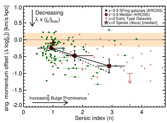
Figure 9: Specific angular momentum offset (see Section 4.3.1) as a function of Sérsic index for the KROSS sample and $z$=0 early-type galaxies. The large data points show the running median and bootstrap errors. The dashed line shows the same running median but using $j_{n=0}$ for all galaxies (see Section 4.3). The shaded region represents the 0.2 dex scatter expected for the distribution of halo spins, $\lambda$. The downward arrow represents the median systematic offset to apply to the $z$=0 early-type galaxies when using an alternative stellar mass fraction to the disks (see Section 4.3). On average, galaxies with higher Sérsic indices (a proxy for bulge fraction) have lower specific angular momentum at both redshifts.

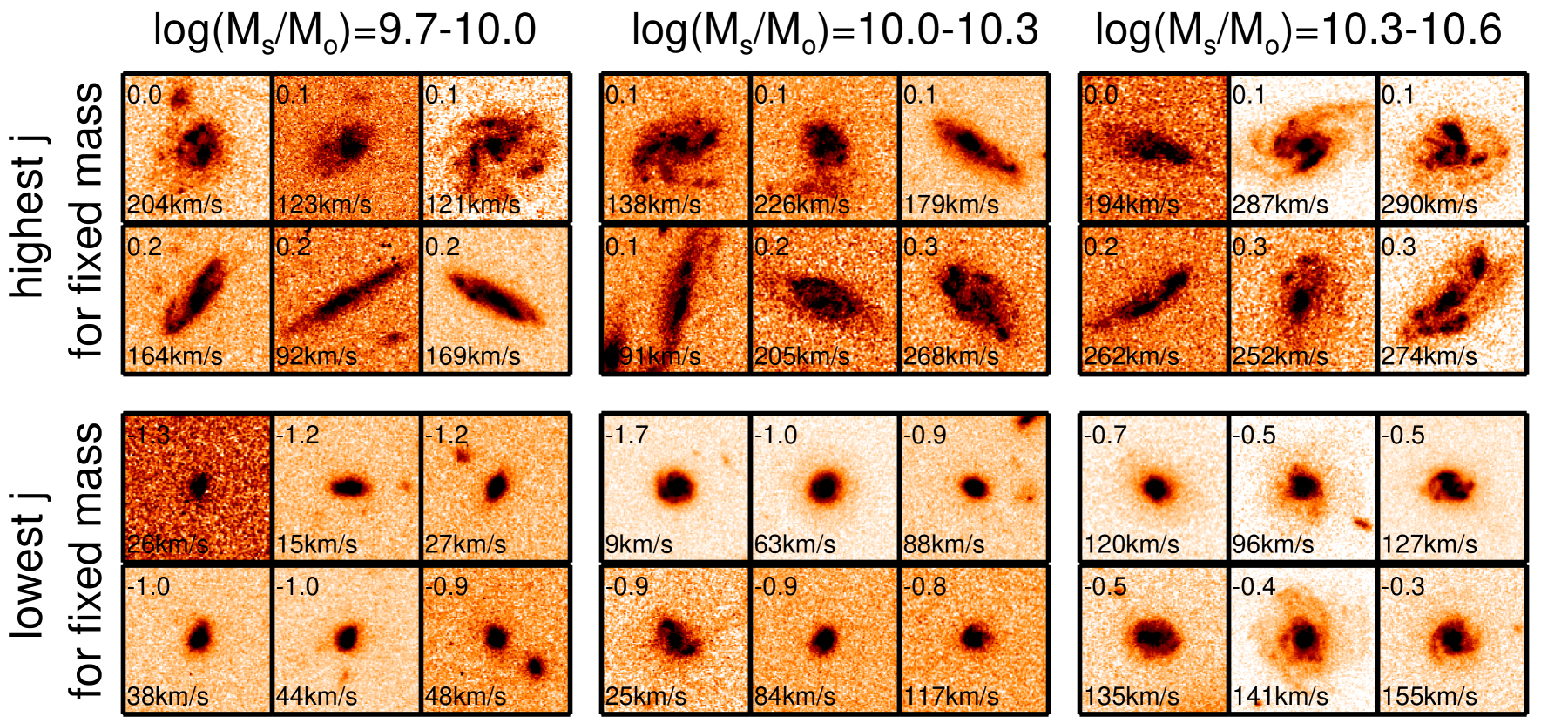
Figure 10: $I$-band HST images for the six lowest (lower panels) and six highest (upper panels) specific angular momentum for a given stellar mass (i.e., $\Delta\log(j_{s})$; see Section 4.4) in three narrow stellar mass bins (columns). The inset numbers in each panel show the $\Delta\log(j_{s})$ values (upper left) and rotational velocity (bottom left) for each target. For a given stellar mass, $z$$\approx$0.9 galaxies with the highest specific angular momentum result in disk-dominated morphologies, whilst those with the lowest specific angular momentum are bulge dominated. These results imply that a momentum–mass–morphology relationship is already in place by this epoch.

Figure 7 shows a large scatter of $\approx$0.4 dex in the $j_{s}$-$M_{\star}$ relationship for $z$$\approx$0.9 star-forming galaxies. Observational results at $z$$\approx$0 find that the $j_{s}$–$M_{\star}$ relationship varies across different morphological types, with later types typically having more angular momentum for a fixed stellar mass (e.g., Sandage et al. 1970; Fall 1983; Romanowsky & Fall 2012; Cortese et al. 2016). Furthermore, Obreschkow & Glazebrook (2014) find that their 16 late-type galaxies follow a relatively tight plane in $M$–$j$–($B$/$T$) space where ($B$/$T$) is the bulge fraction. Under the assumption that the parent halos have the same distribution of spin values, the difference in angular momentum as a function of morphology may indicate a difference in retention of angular momentum due to different contributions of mergers or a varying re-distribution of angular momentum from inflows, outflows and turbulence (see Section 4.3.1; e.g., Zavala et al. 2008; Romanowsky & Fall 2012). Here we explore whether a morphological dependence on $j_{s}$ is already in place by $z$$\approx$1.

Firstly, we can see a there is a clear difference in the normalisation of the $j_{s}$–$M_{\star}$ relationship between the dispersion-dominated and rotationally-dominated galaxies (see Figure 7). Fixing the slope to $\alpha$=0.62, as observed for the sample as a whole, and refitting the relationships as in Section 4.3, the normalisation of the relationship for the dispersion-dominated sources is $\beta_{[v/\sigma<1]}$=2.11$\pm$0.08, corresponding to a $\approx$0.6 dex offset to the rotationally dominated sources ($\beta_{[v/\sigma>1]}$=2.70$\pm$0.03). This is in broad agreement with a model that “diskier" galaxies have more angular momentum per unit mass (e.g., Fall 1983) and the high-redshift IFU results on star-forming galaxies of Burkert et al. (2016). However, whilst $v_{C}$/$\sigma$ is a crude proxy for galaxy type, and this trend is in broad agreement with the predicted $z$=0 trends from the EAGLE hydrodynamical cosmological simulation (Lagos et al. 2016), $v_{C}$ is used in both the calculation of $j_{s}$ (i.e., Equation 5) and the classification of the galaxies. Therefore, this conclusion if subject to strong internal dependencies and in the following we instead focus on an independent proxy for galaxy morphology, the Sérsic index, $n$.

Although our sample is dominated by star-forming, “disky" sources due to our selection criteria (see Section 2.1 and Section 4.1; also see Cortese et al. 2016), we have sources with a range of Sérsic indices ($n$$\approx$0.5–3) based on the subset of our sources with $H$-band HST imaging and the fits of van der Wel et al. (2012) (see Section 3.1.2). Although not tightly correlated with bulge-to-total mass ratios, sources with higher Sérsic indices have more prominent bulges on average. We re-calculate the specific angular momentum, as $j_{n}$, using the individual $n$ values (Equation 5 and Equation 6) for the 101 galaxies which are in our final sample and van der Wel et al. (2012). In Figure 9 we plot these values as an angular momentum offset, $\Delta\log(j_{n})$, from the “model prediction" for angular momentum, $j_{{\rm s,pred}}$ in Equation 7 (setting $f_{j}=1$). We note that the global observed trends are the same if we instead define the offset as being from the $z$=0 $j_{s}$–$M_{\star}$ relationship for spiral galaxies. We also show the early-type galaxies from Romanowsky & Fall (2012) (see Section 2.5). On average, galaxies have decreasing angular momentum for increasing Sérsic index, for a fixed stellar mass (also see Figure 5 in Burkert et al. 2016). There is a factor $\approx$3 decrease in specific angular momentum between $n$=1 and $n$=3. This implies that earlier-type galaxies have less angular momentum compared to later type galaxies at $z$$\approx$1, in agreement with the $z$=0 observations (e.g., Romanowsky & Fall 2012; Cortese et al. 2016).

It is worth noting that Cortese et al. (2016) find a weaker trend between specific angular momentum and Sérsic index when using gas angular momentum, compared to using stellar angular momentum for $z<0.1$ galaxies. Although this may be partly due to Cortese et al. (2016) only investigating the angular momentum within 1$\times$$R_{1/2}$, this may imply that the trend we observed in Figure 9 would be stronger if we had stellar kinematic information available. Furthermore, if we a apply a morphological dependent stellar mass fraction, $f_{s}$, (cf. Dutton et al. 2010; see Section 4.3.1) this would increase the observed trend in Figure 9. Finally, Fall & Romanowsky (2013) find that the strength of the $j$–morphology trend is increased when using colour-dependant mass-to-light ratios as opposed to the fixed mass-to-light ratios used in Romanowsky & Fall (2012). This effect would also strengthen our conclusion on the existence of a specific angular momentum–morphology trend at $z$$\approx$1.

To investigate the specific angular momentum morphology connection further we performed a visual inspection of the broad-band images for the galaxies with the lowest and highest specific angular momentum for their mass (see Figure 8). We considered only the targets with HST imaging (see Section 3.1.1), where visual classification is possible. To avoid any underlying mass dependencies, we split the sample into three mass bins of $9.7\leq\log(M_{\star}[M_{\odot}])<10.0$; $10.0\leq\log(M_{\star}[M_{\odot}])<10.3$ and $10.3\leq\log(M_{\star}[M_{\odot}])<10.6$. In each mass bin we looked at the images for the targets with the lowest specific angular momentum for their mass and those with the highest specific angular momentum for their mass (i.e., lowest and highest $\Delta\log j_{\rm s}$ values). In Figure 10 we show the six highest and six lowest for each mass bin. The galaxies with the lowest specific angular momentum for their mass exhibit small round “bulge” dominated morphologies, whilst those with the highest specific angular momentum for their mass show morphologies dominated by large disks. These qualitative results are consistent with our more quantitative analyses, described above, using the Sérsic indices.

In the context of the simple model outlined in Section 4.3.1 the interpretation here is that galaxies with lower specific angular momentum with respect to the halo (i.e., lower $f_{j}=j_{s}/j_{\rm halo}$ values) and/or with lower halo spins ($\lambda$) result in earlier-type morphologies, i.e., more dominant “bulges”. This is in agreement with the conclusions based on local galaxies of Fall & Romanowsky (2013), who suggest that $f_{j}$ is 8$\times$ larger for $z$=0 disks compared to $z$=0 ellipticals following similar assumptions to those outlined here. Furthermore, it is also in qualitative agreement with numerical model predictions (e.g., Zavala et al. 2016; Teklu et al. 2015). Overall, if the specific angular momentum is indeed the fundamental driver of the Hubble sequence of morphological type (e.g., Romanowsky & Fall 2012; Obreschkow & Glazebrook 2014) our results are in agreement with a model in which the Hubble sequence was already in place, or at least being formed, by $z$$\approx$1 (see e.g., van den Bergh et al. 1996; Simard et al. 1999; Bell et al. 2004; Cassata et al. 2007; Lee et al. 2013).

5 Conclusions

We have presented new measurements and results based on IFU data of $\approx$600 H$\alpha$ detected $z$=0.6–1.0 star-forming galaxies that were observed as part of KROSS (Stott et al. 2016). These sources are representative of $\log\left(M_{\star}[{\rm M_{\odot}}]\right)\approx$ 9–11 star-forming galaxies at this redshift. Using a combination of broad-band imaging and our IFU data we have made measurements of inclination angles, half-light radii, morphological and kinematic position angles, rotational velocities, intrinsic velocity dispersions and specific angular momentum. Our main conclusions are:

• The sample is dominated by galaxies that have rotationally-dominated gas kinematics, with rotational velocities that are greater than their intrinsic velocity dispersion. We measure $v_{C}/\sigma_{0}>1$ for 81$\pm$5 per cent of the sources in our sample that have spatially-resolved velocity measurements.

• For the rotationally-dominated systems we find a correlation between rotational velocity and mass (i.e., the inverted stellar mass Tully-Fisher Relationship) that is consistent with $z=0$ disks with $\log v=2.12\pm 0.04+(0.33\pm 0.11)[\log(M_{\star}/$M${}_{\odot})-10.1]$. The dispersion-dominated systems scatter below this trend (Figure 6).

• The specific angular momentum (angular momentum divided by stellar mass; $j_{s}$) at $z$$\approx$1 is related to stellar mass following $\log j_{s}=2.59\pm 0.04+(0.6\pm 0.2)[\log(M_{\star}[$M${}_{\odot}])-10.1]$.

• The observed scaling relationship, $j_{s}\propto M_{\star}^{0.6\pm 0.2}$, is in agreement with local disks and the scaling relationship between angular momentum and mass expected for dark matter, i.e., $j_{\rm DM}\propto M_{\rm DM}^{2/3}$ (Figure 7). This implies little mass dependence on the conversion between halo angular momentum and galaxy angular momentum, on average, for this sample.

• The normalisation of the $j_{s}$–$M_{\star}$ relationship is $\approx$0.2–0.3 dex lower in our sample compared to z$=$0 disk galaxies (Figure 7). A difference in galaxy sizes, for a fixed stellar mass, is the primary driver of this evolution as $j_{s}\propto R_{D}v_{C}$ and we do not observe an evolution in the rotational velocity–mass relationship.

• In the context of an idealised isothermal halo model, with fixed spin parameter, $\lambda$=0.035, the median ratio of specific angular momentum between the galaxy and halo is $j_{s}/j_{{\rm halo}}$$\approx$50–60 per cent for the rotationally-dominated KROSS galaxies (Figure 8). These $z\approx 0.9$ galaxies show only a small offset of $\approx$0.1–0.2 dex to lower values of this ratio compared to $z$=0 disks, despite a significant difference in host-galaxy properties such as average star-formation rates.

• The observed galaxies have less angular momentum with increasing Sérsic index at a fixed stellar mass, with a factor of $\approx$3 decrease in average $j_{s}$ between $n$=1 and $n$=3 (Figure 9). Furthermore, the sources with the highest specific angular momentum at any given mass have the visually most disk-dominated morphologies (Figure 10). This reveals that angular momentum may be key in determining a galaxy’s morphology and an angular momentum–mass–morphology relationship is already in place by $z\approx 1$.

Acknowledgements

We thank the referee for their constructive comments. We acknowledge the Science and Technology Facilities Council (CMH, AMS, RGB and RMS through grant code ST/L00075X/1). AMS acknowledges the Leverhulme Foundation. JPS, MB and MJJ acknowledges support from a Hintze Research Fellowship. IRS acknowledges support from an ERC Advanced Investigator programme DUSTYGAL 321334 and a Royal Society/Wolfson Merit Award. AJB gratefully acknowledges the hospitality of the Research School of Astronomy & Astrophysics at the Australian National University, Mount Stromlo, Canberra. DS acknowledges financial support from the Netherlands Organisation for Scientific research (NWO) through a Veni fellowship and Lancaster University through an Early Career Internal Grant (A100679). GEM acknowledges support from the ERC Consolidator Grant funding scheme (project ConTExt, grant number No. 648179) and a research grant (13160) from Villum Fonden. This work is based on observations taken by the CANDELS Multi-Cycle Treasury Program with the NASA/ESA HST, which is operated by the Association of Universities for Research in Astronomy, Inc., under NASA contract NAS5-26555. HST data were also obtained from the data archive at the Space Telescope Science Institute. We thank Holly Elbert, Timothy Green and Laura Prichard for carrying out some observations.

Appendix A Catalogue

With this paper we release a catalogue of raw and derived values for the 586 H$\alpha$ detected targets. This is available in electronic format at http://astro.dur.ac.uk/KROSS, where later releases and updates will also be placed. The full version of Figure 2 and the H$\alpha$ emission-line profiles for all detected targets are also available at the same location. In Table 1 we describe the columns of the catalogue released with this paper.

Descriptions of Columns

Number	Name	Units	Description
1	ID		KROSS ID.
2	NAME		Object Name.
3	RA		Right Ascension (J2000).
4	DEC		Declination (J2000).
5	K_AB		$K$-band magnitude (AB).
6	R_AB		$r$-band magnitude (AB).
7	Z_AB		$z$-band magnitude (AB).
8	M_H		Absolute $H$-band magnitude.
9	MASS	M⊙	Stellar mass, scaled from $M_{H}$ with a fixed mass-to-light ratio.
10	VDW12_N		Sérsic index $n$ from van der Wel et al. (2012).
11	IM_TYPE		Band of broad-band image used in the analyses.
12	QUALITY_FLAG		Quality flag for the data:
			Quality 1: H$\alpha$ detected, spatially-resolved and both $\theta_{\rm im}$ and $R_{1/2}$ were measured from the broad-band
			Quality 2: H$\alpha$ detected and spatially resolved but $\theta_{\rm im}$ was fixed (see THETA_FLAG) and/or $R_{1/2}$ was
			estimated from the kinematic (see R_FLAG)
			Quality 3: H$\alpha$ detected and resolved in the IFU data but only an upper limit on $R_{1/2}$
			Quality 4: H$\alpha$ detected but unresolved in the IFU data.
13	PA_IM	degrees	Positional angle of the broad-band image, PAim.
14–15	R_IM	kpc	Deconvolved continuum half-light radii, $R_{1/2}$, from the image and error.
16	R_FLAG		If $=$1 then $R_{1/2}$ is an upper limit, if $=$0.5 then $R_{1/2}$ was estimated using a fit to the kinematic data.
17	B_O_A		The observed axis ratio $b/a$ from the broad-band image.
18–19	THETA_IM	degrees	The inferred inclination angle, $\theta_{\rm im}$, with error. If $\theta_{\rm im}<25$ then excluded from the analyses.
20	THETA_FLAG		If $=$1 then the inclination angle was fixed to 53${}^{\rm o}\pm 18$.
21	Z		Redshift from H$\alpha$.
22	F_HA	erg s-1 cm-2	Observed aperture H$\alpha$ flux.
23	L_HA	erg s-1	Observed H$\alpha$ luminosity with a factor $\times$1.5 aperture correction applied
24	SFR	M⊙ yr-1	Inferred star-formation rate from H$\alpha$ luminosity and applying an Av correction.
25	SIGMA_TOT	km s-1	Velocity dispersion $\sigma_{\rm tot}$ from the galaxy-integrated (aperture) spectrum.
26	AGN_FLAG		If $=$1 AGN emission affecting the emission-line properties and are excluded from the final analyses.
27	IRR_FLAG		If $=$1 unphysical measurements for the rotational velocities and/or the half-light radii
			and are excluded from the final analyses.
28	VEL_PA	degrees	Position angle of the major kinematic axis, PAvel.
29	V22_OBS	km s-1	Observed velocity measured at 1.3 R1/2 (i.e., $\approx$2.2 RD), $v_{2.2}$.
30	V22	km s-1	Intrinsic $v_{2.2}$ after inclination and beam-smearing corrections.
31	VC_OBS	km s-1	Observed velocity measured at 2 R1/2 (i.e., $\approx$3.4 RD), $v_{C}$.
32–34	VC	km s-1	Intrinsic $v_{C}$ after inclination and beam-smearing corrections, with lower and upper errors.
35	EXTRAP_FLAG		If $=$1, $v_{C}$ extrapolated $>$2 pixels beyond the extent of the data, if $=$2 then $v_{C}$ was estimated by scaling $\sigma_{\rm tot}$.
36	KIN_TYPE		Kinematic classification: RT$+$ “gold” rotationally dominated; RT: rotationally dominated;
			DN: dispersion dominated; X: IFU data is spatially unresolved;
37–39	JS	km  s-1 kpc	Specific angular momentum, $j_{s}$, with lower and upper errors. Negative values correspond to upper limits.
40	JN	km  s-1 kpc	Specific angular momentum, $j_{n}$, using individual $n$ values.

Table 1: Details of the columns provided in the public release of the KROSS catalogue associated with this paper. We note that the quoted errors are conservative and take into account systematic uncertainties due to the methods applied and effects due to the varying quality of data across the sample (see details in Section 3).

References

- Abadi et al. (2003) Abadi M. G., Navarro J. F., Steinmetz M., Eke V. R., 2003, ApJ, 591, 499
- Agertz et al. (2011) Agertz O., Teyssier R., Moore B., 2011, MNRAS, 410, 1391
- Amanullah et al. (2010) Amanullah R., et al., 2010, ApJ, 716, 712
- Barnes & Efstathiou (1987) Barnes J., Efstathiou G., 1987, ApJ, 319, 575
- Bell & de Jong (2001) Bell E. F., de Jong R. S., 2001, ApJ, 550, 212
- Bell et al. (2004) Bell E. F., et al., 2004, ApJL, 600, L11
- Bershady et al. (2011) Bershady M. A., Martinsson T. P. K., Verheijen M. A. W., Westfall K. B., Andersen D. R., Swaters R. A., 2011, ApJL, 739, L47
- Bertola & Capaccioli (1975) Bertola F., Capaccioli M., 1975, ApJ, 200, 439
- Bett et al. (2007) Bett P., Eke V., Frenk C. S., Jenkins A., Helly J., Navarro J., 2007, MNRAS, 376, 215
- Blumenthal et al. (1984) Blumenthal G. R., Faber S. M., Primack J. R., Rees M. J., 1984, Nature, 311, 517
- Bolzonella et al. (2000) Bolzonella M., Miralles J.-M., Pelló R., 2000, A&A, 363, 476
- Bouché et al. (2007) Bouché N., et al., 2007, ApJ, 671, 303
- Brook et al. (2012) Brook C. B., Stinson G., Gibson B. K., Roškar R., Wadsley J., Quinn T., 2012, MNRAS, 419, 771
- Bruzual & Charlot (2003) Bruzual G., Charlot S., 2003, MNRAS, 344, 1000
- Bryant et al. (2015) Bryant J. J., et al., 2015, MNRAS, 447, 2857
- Bundy et al. (2015) Bundy K., et al., 2015, ApJ, 798, 7
- Burkert et al. (2010) Burkert A., et al., 2010, ApJ, 725, 2324
- Burkert et al. (2016) Burkert A., et al., 2016, ApJ, 826, 214
- Cappellari et al. (2011) Cappellari M., et al., 2011, MNRAS, 413, 813
- Cassata et al. (2007) Cassata P., et al., 2007, ApJS, 172, 270
- Catelan & Theuns (1996) Catelan P., Theuns T., 1996, MNRAS, 282, 436
- Chabrier (2003) Chabrier G., 2003, PASP, 115, 763
- Conselice et al. (2005) Conselice C. J., Bundy K., Ellis R. S., Brichmann J., Vogt N. P., Phillips A. C., 2005, ApJ, 628, 160
- Contini et al. (2016) Contini T., et al., 2016, A&A, 591, A49
- Cortese et al. (2014) Cortese L., et al., 2014, ApJL, 795, L37
- Cortese et al. (2016) Cortese L., et al., 2016, preprint, (arXiv:1608.00291)
- Courteau (1997) Courteau S., 1997, AJ, 114, 2402
- Covington et al. (2010) Covington M. D., et al., 2010, ApJ, 710, 279
- Crain et al. (2015) Crain R. A., et al., 2015, MNRAS, 450, 1937
- Danovich et al. (2015) Danovich M., Dekel A., Hahn O., Ceverino D., Primack J., 2015, MNRAS, 449, 2087
- Davies et al. (2013) Davies R. I., et al., 2013, A&A, 558, A56
- Dekel et al. (2009) Dekel A., Sari R., Ceverino D., 2009, ApJ, 703, 785
- Di Teodoro et al. (2016) Di Teodoro E. M., Fraternali F., Miller S. H., 2016, preprint, (arXiv:1602.04942)
- Dubois et al. (2014) Dubois Y., et al., 2014, MNRAS, 444, 1453
- Dutton et al. (2010) Dutton A. A., Conroy C., van den Bosch F. C., Prada F., More S., 2010, MNRAS, 407, 2
- Dutton et al. (2011) Dutton A. A., et al., 2011, MNRAS, 410, 1660
- Eke et al. (2000) Eke V., Efstathiou G., Wright L., 2000, MNRAS, 315, L18
- Emsellem et al. (2007) Emsellem E., et al., 2007, MNRAS, 379, 401
- Epinat et al. (2010) Epinat B., Amram P., Balkowski C., Marcelin M., 2010, MNRAS, 401, 2113
- Fall (1983) Fall S. M., 1983, in Athanassoula E., ed., IAU Symposium Vol. 100, Internal Kinematics and Dynamics of Galaxies. pp 391–398
- Fall & Efstathiou (1980) Fall S. M., Efstathiou G., 1980, MNRAS, 193, 189
- Fall & Romanowsky (2013) Fall S. M., Romanowsky A. J., 2013, ApJL, 769, L26
- Ferrero et al. (2016) Ferrero I., et al., 2016, preprint, (arXiv:1607.03100)
- Flores et al. (2006) Flores H., Hammer F., Puech M., Amram P., Balkowski C., 2006, A&A, 455, 107
- Förster Schreiber et al. (2006) Förster Schreiber N. M., et al., 2006, ApJ, 645, 1062
- Franx et al. (1991) Franx M., Illingworth G., de Zeeuw T., 1991, ApJ, 383, 112
- Freeman (1970) Freeman K. C., 1970, ApJ, 160, 811
- Genel et al. (2015) Genel S., Fall S. M., Hernquist L., Vogelsberger M., Snyder G. F., Rodriguez-Gomez V., Sijacki D., Springel V., 2015, ApJL, 804, L40
- Genzel et al. (2006) Genzel R., et al., 2006, Nature, 442, 786
- Giacconi et al. (2001) Giacconi R., et al., 2001, ApJ, 551, 624
- Governato et al. (2007) Governato F., Willman B., Mayer L., Brooks A., Stinson G., Valenzuela O., Wadsley J., Quinn T., 2007, MNRAS, 374, 1479
- Grogin et al. (2011) Grogin N. A., et al., 2011, ApJS, 197, 35
- Guo et al. (2010) Guo Q., White S., Li C., Boylan-Kolchin M., 2010, MNRAS, 404, 1111
- Harrison et al. (2016) Harrison C. M., et al., 2016, MNRAS, 456, 1195
- Heavens & Peacock (1988) Heavens A., Peacock J., 1988, MNRAS, 232, 339
- Kannappan et al. (2002) Kannappan S. J., Fabricant D. G., Franx M., 2002, AJ, 123, 2358
- Kassin et al. (2007) Kassin S. A., et al., 2007, ApJL, 660, L35
- Kassin et al. (2012) Kassin S. A., et al., 2012, ApJ, 758, 106
- Kennicutt (1998) Kennicutt Jr. R. C., 1998, ARAA, 36, 189
- Kewley et al. (2013) Kewley L. J., Dopita M. A., Leitherer C., Davé R., Yuan T., Allen M., Groves B., Sutherland R., 2013, ApJ, 774, 100
- Khandai et al. (2015) Khandai N., Di Matteo T., Croft R., Wilkins S., Feng Y., Tucker E., DeGraf C., Liu M.-S., 2015, MNRAS, 450, 1349
- Kimm et al. (2011) Kimm T., Devriendt J., Slyz A., Pichon C., Kassin S. A., Dubois Y., 2011, preprint, (arXiv:1106.0538)
- Koekemoer et al. (2011) Koekemoer A. M., et al., 2011, ApJS, 197, 36
- Lagos et al. (2016) Lagos C. d. P., Theuns T., Stevens A. R. H., Cortese L., Padilla N. D., Davis T. A., Contreras S., Croton D., 2016, preprint, (arXiv:1609.01739)
- Law et al. (2012) Law D. R., Steidel C. C., Shapley A. E., Nagy S. R., Reddy N. A., Erb D. K., 2012, ApJ, 745, 85
- Lawrence et al. (2007) Lawrence A., et al., 2007, MNRAS, 379, 1599
- Leauthaud et al. (2007) Leauthaud A., et al., 2007, ApJS, 172, 219
- Lee et al. (2013) Lee B., et al., 2013, ApJ, 774, 47
- Lehmer et al. (2005) Lehmer B. D., et al., 2005, ApJS, 161, 21
- Macciò et al. (2008) Macciò A. V., Dutton A. A., van den Bosch F. C., 2008, MNRAS, 391, 1940
- Magdis et al. (2016) Magdis G. E., et al., 2016, MNRAS, 456, 4533
- Markwardt (2009) Markwardt C. B., 2009, in Bohlender D. A., Durand D., Dowler P., eds, Astronomical Society of the Pacific Conference Series Vol. 411, Astronomical Data Analysis Software and Systems XVIII. p. 251 (arXiv:0902.2850)
- Mason et al. (2016) Mason C. A., et al., 2016, preprint, (arXiv:1610.03075)
- Miller et al. (2011) Miller S. H., Bundy K., Sullivan M., Ellis R. S., Treu T., 2011, ApJ, 741, 115
- Miller et al. (2013) Miller S. H., Sullivan M., Ellis R. S., 2013, ApJL, 762, L11
- Mo et al. (1998) Mo H. J., Mao S., White S. D. M., 1998, MNRAS, 295, 319
- Mo et al. (2010) Mo H., van den Bosch F. C., White S., 2010, Galaxy Formation and Evolution
- Navarro & Steinmetz (1997) Navarro J. F., Steinmetz M., 1997, ApJ, 478, 13
- Navarro et al. (1995) Navarro J. F., Frenk C. S., White S. D. M., 1995, MNRAS, 275, 56
- Obreschkow & Glazebrook (2014) Obreschkow D., Glazebrook K., 2014, ApJ, 784, 26
- Obreschkow et al. (2015) Obreschkow D., Meyer M., Popping A., Power C., Quinn P., Staveley-Smith L., 2015, Advancing Astrophysics with the Square Kilometre Array (AASKA14), p. 138
- Osterbrock & Ferland (2006) Osterbrock D. E., Ferland G. J., 2006, Astrophysics of Gaseous Nebulae and Active Galactic Nuclei, Univ. Science Books, Mill Valley, CA
- Paturel et al. (2003) Paturel G., Petit C., Prugniel P., Theureau G., Rousseau J., Brouty M., Dubois P., Cambrésy L., 2003, A&A, 412, 45
- Peebles (1969) Peebles P. J. E., 1969, ApJ, 155, 393
- Peebles (1971) Peebles P. J. E., 1971, A&A, 11, 377
- Pelliccia et al. (2016) Pelliccia D., Tresse L., Epinat B., Ilbert O., Scoville N., Amram P., Lemaux B. C., Zamorani G., 2016, preprint, (arXiv:1606.01934)
- Pizagno et al. (2007) Pizagno J., et al., 2007, AJ, 134, 945
- Portinari & Sommer-Larsen (2007) Portinari L., Sommer-Larsen J., 2007, MNRAS, 375, 913
- Puech et al. (2007) Puech M., Hammer F., Lehnert M. D., Flores H., 2007, A&A, 466, 83
- Puech et al. (2010) Puech M., Hammer F., Flores H., Delgado-Serrano R., Rodrigues M., Yang Y., 2010, A&A, 510, A68
- Rees & Ostriker (1977) Rees M. J., Ostriker J. P., 1977, MNRAS, 179, 541
- Reyes et al. (2011) Reyes R., Mandelbaum R., Gunn J. E., Pizagno J., Lackner C. N., 2011, MNRAS, 417, 2347
- Rix et al. (2004) Rix H.-W., et al., 2004, ApJS, 152, 163
- Romanowsky & Fall (2012) Romanowsky A. J., Fall S. M., 2012, ApJS, 203, 17
- Rousselot et al. (2000) Rousselot P., Lidman C., Cuby J.-G., Moreels G., Monnet G., 2000, A&A, 354, 1134
- Sánchez et al. (2012) Sánchez S. F., et al., 2012, A&A, 538, A8
- Sandage et al. (1970) Sandage A., Freeman K. C., Stokes N. R., 1970, ApJ, 160, 831
- Scannapieco et al. (2008) Scannapieco C., Tissera P. B., White S. D. M., Springel V., 2008, MNRAS, 389, 1137
- Scannapieco et al. (2012) Scannapieco C., et al., 2012, MNRAS, 423, 1726
- Schaye et al. (2015) Schaye J., et al., 2015, MNRAS, 446, 521
- Schreiber et al. (2015) Schreiber C., et al., 2015, A&A, 575, A74
- Scoville et al. (2007) Scoville N., et al., 2007, ApJS, 172, 1
- Sharples et al. (2004) Sharples R. M., et al., 2004, in Moorwood A. F. M., Iye M., eds, Society of Photo-Optical Instrumentation Engineers (SPIE) Conference Series Vol. 5492, Ground-based Instrumentation for Astronomy. pp 1179–1186, doi:10.1117/12.550495
- Sharples et al. (2013) Sharples R., et al., 2013, The Messenger, 151, 21
- Shaya & Tully (1984) Shaya E. J., Tully R. B., 1984, ApJ, 281, 56
- Silk (1997) Silk J., 1997, ApJ, 481, 703
- Simard et al. (1999) Simard L., et al., 1999, ApJ, 519, 563
- Simons et al. (2015) Simons R. C., Kassin S. A., Weiner B. J., Heckman T. M., Lee J. C., Lotz J. M., Peth M., Tchernyshyov K., 2015, MNRAS, 452, 986
- Sobral et al. (2013a) Sobral D., Smail I., Best P. N., Geach J. E., Matsuda Y., Stott J. P., Cirasuolo M., Kurk J., 2013a, MNRAS, 428, 1128
- Sobral et al. (2013b) Sobral D., et al., 2013b, ApJ, 779, 139
- Sobral et al. (2015) Sobral D., et al., 2015, MNRAS, 451, 2303
- Sommer-Larsen et al. (2003) Sommer-Larsen J., Götz M., Portinari L., 2003, ApJ, 596, 47
- Speagle et al. (2014) Speagle J. S., Steinhardt C. L., Capak P. L., Silverman J. D., 2014, ApJS, 214, 15
- Steidel et al. (1998) Steidel C. C., Adelberger K. L., Dickinson M., Giavalisco M., Pettini M., Kellogg M., 1998, ApJ, 492, 428
- Stevens et al. (2016) Stevens A. R. H., Croton D. J., Mutch S. J., 2016, MNRAS, 461, 859
- Stewart et al. (2013) Stewart K. R., Brooks A. M., Bullock J. S., Maller A. H., Diemand J., Wadsley J., Moustakas L. A., 2013, ApJ, 769, 74
- Stott et al. (2014) Stott J. P., et al., 2014, MNRAS, 443, 2695
- Stott et al. (2016) Stott J. P., et al., 2016, MNRAS, 457, 1888
- Tasca et al. (2009) Tasca L. A. M., et al., 2009, A&A, 503, 379
- Teklu et al. (2015) Teklu A. F., Remus R.-S., Dolag K., Beck A. M., Burkert A., Schmidt A. S., Schulze F., Steinborn L. K., 2015, ApJ, 812, 29
- Thacker & Couchman (2001) Thacker R. J., Couchman H. M. P., 2001, ApJL, 555, L17
- Tiley et al. (2016) Tiley A. L., et al., 2016, MNRAS, 460, 103
- Torrey et al. (2014) Torrey P., Vogelsberger M., Genel S., Sijacki D., Springel V., Hernquist L., 2014, MNRAS, 438, 1985
- Tully & Fisher (1977) Tully R. B., Fisher J. R., 1977, A&A, 54, 661
- Übler et al. (2014) Übler H., Naab T., Oser L., Aumer M., Sales L. V., White S. D. M., 2014, MNRAS, 443, 2092
- Vergani et al. (2012) Vergani D., et al., 2012, A&A, 546, A118
- Vogelsberger et al. (2014) Vogelsberger M., et al., 2014, MNRAS, 444, 1518
- Weijmans et al. (2014) Weijmans A.-M., et al., 2014, MNRAS, 444, 3340
- Weil et al. (1998) Weil M. L., Eke V. R., Efstathiou G., 1998, MNRAS, 300, 773
- Weiner et al. (2006) Weiner B. J., et al., 2006, ApJ, 653, 1027
- White (1984) White S. D. M., 1984, ApJ, 286, 38
- White & Frenk (1991) White S. D. M., Frenk C. S., 1991, ApJ, 379, 52
- Wisnioski et al. (2015) Wisnioski E., et al., 2015, ApJ, 799, 209
- Wuyts et al. (2013) Wuyts S., et al., 2013, ApJ, 779, 135
- Zavala et al. (2008) Zavala J., Okamoto T., Frenk C. S., 2008, MNRAS, 387, 364
- Zavala et al. (2016) Zavala J., et al., 2016, MNRAS, 460, 4466
- Zjupa & Springel (2016) Zjupa J., Springel V., 2016, preprint, (arXiv:1608.01323)
- van den Bergh et al. (1996) van den Bergh S., Abraham R. G., Ellis R. S., Tanvir N. R., Santiago B. X., Glazebrook K. G., 1996, AJ, 112, 359
- van der Wel et al. (2012) van der Wel A., et al., 2012, ApJS, 203, 24
- van der Wel et al. (2014) van der Wel A., et al., 2014, ApJ, 788, 28