Spitzer’s View of the Candidate Cluster and Protocluster Catalog (CCPC)

Abstract

The Candidate Cluster and Protocluster Catalog (CCPC) contains 218 galaxy overdensities composed of more than 2000 galaxies with spectroscopic redshifts spanning the first few Gyrs after the Big Bang $(2.0\leq z<6.6)$. We use Spitzer archival data to track the underlying stellar mass of these overdense regions in various temporal cross sections by building rest-frame near-infrared luminosity functions across the span of redshifts.This exercise maps the stellar growth of protocluster galaxies, as halos in the densest environments should be the most massive from hierarchical accretion. The characteristic apparent magnitude, $m^{*}(z)$, is relatively flat from $2.0\leq z<6.6$, consistent with a passive evolution of an old stellar population. This trend maps smoothly to lower redshift results of cluster galaxies from other works. We find no difference in the luminosity functions of galaxies in the field versus protoclusters at a given redshift, apart from their density.

1. Introduction

The nascent study of protoclusters is at a juncture of two important evolutionary epochs in the universe: the early growth of large structures and the rapid assembly of galaxy mass at $z\geq 2$. Careful study of these objects can probe both cosmology and galaxy formation and evolution. The initial mass overdensities in the early universe (and their subsequent collapse) are governed by the cosmic matter density ($\Omega_{\mathrm{m}}$), $\sigma_{8}$, and the cosmological constant $\Omega_{\mathrm{\Lambda}}$. Thus, by examining their properties (mass, evolutionary state) and number density of these early structures, they can provide constraints on these cosmological parameters. The tracers of these overdense structures (i.e., galaxies) can be used to investigate the role environment plays in their growth and evolution. Formation models of galaxies must match observations across both cosmic time and throughout space to be considered viable. More simply, void and cluster galaxies must both be reproduced for all $z\geq 0$. The focus of this work will be primarily on the properties of galaxies in dense environments, but this juncture of structure and galaxy evolution are clearly relatable in many ways.

It has been clear for many decades that galaxies at $z=0$ have varied properties that correlate strongly with density in the well-established morphology-density relation (dre80; bal04). Galaxies in dense environments show clear evolution at higher redshift (but84), in that there are more passive galaxies in local clusters, but a greater fraction of star forming objects in higher redshift systems. This can be seen observationally in the fraction of quiescent, ‘red-sequence’ objects in contrast with the ‘blue cloud’ of star forming galaxies (SFGs) as a function of redshift (sta95; rak95). These two facts provide an initial scaffolding from which galaxy evolutionary models can be wrought: quiescent systems dominate high density regions of the local universe, and this need not hold throughout cosmic time. What is the path that must be taken to satisfy these two simple observations?

One prescription to turn these observational facts into a coherent model is to identify physical processes that effectively turn SFGs into quiescent systems preferentially in dense environments. Commonly invoked interactions are ram-pressure stripping of cold gas by the intracluster medium (ICM; gun72), removal of the hot gas halo of a galaxy to halt the cooling of gas to sustain star formation (e.g. strangulation; lar80), galaxy-galaxy interactions that disrupt the galaxy (moo96), and a variety of others. The overarching umbrella that is used to refer to these proposed mechanisms is called ‘quenching’ (pen10), loosely defined here as the environmental process(es) that abruptly discontinue star formation in a galaxy.

Each proposed quenching process has a distinct time scale at which it can effectively halt star formation. These are generally related to the crossing/dynamical time of the galaxies interacting with other galaxies and/or the ICM. For this latter case, it also assumes that the hot ICM is in place at the epoch in question so as to produce the desired effect. These quenching timescales have been estimated to operate on the order of a few Gyrs for an effective change to manifest itself (bro13). If cluster galaxies are transformed primarily by one quenching mechanisms, it might be possible to examine the galaxy populations in clusters at various cross-sections in time (e.g., redshifts) to isolate the process responsible.

Another proposed scenario used to explain the evolution of the galaxy population in clusters is from galaxy mergers. Hierarchical accretion suggests that galaxies assemble from the bottom up. In the context of clusters, these mergers have been proposed to be either dry (e.g. gas-free; van05) or wet (gas-rich collisions; fab07). In the wet merger scenario, two or more blue cloud galaxies come together in a burst of star formation, turning into a spheroidal configuration (mih96), and are then quenched via some mechanism. This is effectively a transition from the blue cloud onto the red sequence. Dry mergers, on the other hand, push galaxies along the red sequence as they grow in stellar mass, but remain with a generally passive stellar population (color). It is possible and even probable that the various quenching mechanisms and merger scenarios could all play a role of varying importance. Do any observations hint at a timescale of rapid development in the history of cluster galaxies?

The red sequence feature of galaxy clusters has been historically used as a tracer of the core galaxy population at redshifts $z<1.5$ (sta95; rak95; sta98; eis08; mei09). Using models of galaxy colors a mean stellar age of the individual systems can be estimated. Progenitor bias (van01) can ultimately lead to an increased estimated formation redshift ($z_{f}$) for a cluster’s galaxy population as a whole. Despite this caveat, the stellar age of the brightest systems on the red sequence can give some indication as to when the most massive galaxies formed their stars. Models of galaxy growth used to match the evolution of the red sequence feature typically rely on pure, passive evolution models that were formed in a single burst at high redshift $z_{f}>3$ (eis08). In fact, some studies of clusters suggest even larger formation redshifts of $z_{f}>5$ (rak95; sch09). As the redshift of the cluster sample increases, the formation redshift also grows (with an accompanying increase of scatter).

For instance, for cluster redshifts $z>1$, it appears that $z_{f}=30$ is not ruled out (Fig 19 of eis08). Not all cluster galaxies need form at $z_{f}>5$, but at least some passive systems were born remarkably early in the universe. This could simply be a manifestation of galaxy downsizing (cow96), in which the largest stellar mass galaxies (presumably formed in the densest regions) formed earlier in the universe. Within the literature, there is no consensus for any single model or mechanism for the redshift evolution of the red sequence feature (fas14; fri14).

By shifting the focus from the highly biased red sequence galaxies to cluster populations in general, there is the hope that the bulk stellar properties of these systems could be investigated as a function of redshift. man10 mapped the luminosity functions (LFs) of cluster galaxies spanning $0.3<z<2.0$ at Spitzer wavelengths. At the highest redshift of this sample, Spitzer 3.6 $\mu$m coverage measures rest-frame $J$ band, which is a tracer of the stellar population for a range of ages. They mapped the evolution of the characteristic luminosity $m^{*}(z)$ of the clusters by comparing the data to models of simple stellar populations with various formation redshifts $z_{f}$. This is similar to the exercise performed for red-sequence fitting. The mean formation age of these systems was $z_{f}\sim 2.5$ (man10), with the same behavior noted previously: higher redshift clusters favor higher formation redshifts. Their two highest redshift bins ($z\geq 1.5$) have $m^{*}(z)$ values nearly a magnitude fainter than the predicted evolution of their best fitting model (their Fig 7). The conclusion drawn from this observation is that rapid mass assembly (up to $4\times$ growth) must occur in cluster galaxies $z\leq 1.5$ (man10). bro13 investigated the star formation activity of galaxies in these clusters to look for clues as to the nature of this mass assembly. They found that the star formation within the core of these clusters transition from unquenched to quenched at the same epoch ($z\sim 1.4$) as the rapid assembly era within man10. This behavior is generally attributed to wet mergers within the cluster core, rapidly growing the mass of these systems and then abruptly turning off the star formation activity.

In the previous examples, all of the structures were considered to be clusters. Generally speaking, the highest redshift at which virialized halos of $M\geq 10^{14}$ $\,M_{\odot}$(e.g. clusters) are expected is at $z\sim 2$ in large $\Lambda$CDM simulations (chi13). The collection of components that will constitute a cluster in the future is referred to as a protocluster. Observationally, galaxy overdensities at $z>2$ are designated as protoclusters for the sake of simplicity, as it is difficult to confirm these systems to be in virial equilibrium apart from a handful of cases (gob11; wan16). This unique transition point in the universe represents an epoch at which galaxies could first begin to interact with one another. man10 and bro13 presented tantalizing evidence that the majority of mass assembly occurred around $z\sim 1.5$, but higher redshift luminosity functions of structure might yield further insight into the galaxy growth within dense environments.

wyl13 identified Spitzer galaxy overdensities around high redshift ($1.3<z<3.1$) radio-loud AGN and built 3.6 and 4.5 $\mu$m LFs in wyl14. This redshift range overlapped the sample of man10 and extended the age probed by more than 1 Gyr. Remarkably, the $m_{3.6}^{*}$ and $m_{4.5}^{*}$ evolution over the redshifts probed are well fit by a passive stellar evolution model formed at $z_{f}=3$ or larger. They also do not match the results of man10, in that they fail to see a burst of mass assembly at $z\leq 1.5$. This is attributed to a sampling bias, in that the high redshift overdensities are thought to be the most massive, rare systems in the universe, while the lower redshift sample is tracing the growth of less massive clusters. This is analogous to galaxy downsizing, in that the most massive overdensities are fated to assemble into a cluster mass halo more quickly in $\Lambda$CDM (chi13). Therefore, signatures of mass assembly for the progenitor systems of (wyl14) could potentially be observable beyond their redshift limit of $z\approx 3$. In Section 3, we probe these earlier epochs to possibly identify epochs at which rapid mass growth or quenching might be exhibited.

Thus far, it appears that galaxies within clusters, as traced by both red sequence and LF models, form at high redshift ($z_{f}\geq 3$) and evolve passively thereafter. This is an interesting result, as the cosmic star formation rate in the universe does not peak until approximately $z\sim 2$ (mad14). Indeed, if galaxies in dense environments form earlier than their ‘field’ galaxy counterparts, which follow the mean trend, then evidence of this should be apparent at high redshifts. The number of spectroscopically confirmed protoclusters has evolved considerably after the first few discoveries (ste98; ven02), but were still only numbered in the few dozens up until recently. These were also identified by a wide range of selection techniques, from blind spectroscopic surveys (ste98) to targeted narrowband (NB) imaging around high redshift quasars (ven07). In the instances in which these galaxy overdensities were compared with field galaxies at a similar redshift, the results of environmental evolution are varied at best. We continue the exploration of these results at higher redshift in Section LABEL:sec:dis.

The majority of cases in the literature where protocluster galaxies were measured with respect to field sources consist of one or two candidate structures that are compared to a ‘blank’ field-of-view. For instance, cas15 studied a protocluster at $z=2.5$ within the COSMOS field and found that it had evidence of greater AGN activity, more indications of merging/interacting galaxies, and a population of Lyman-Break Galaxies (LBGs) with $\sim 1.5\times$ greater stellar mass. These had similar star formation rates (SFRs) when compared to field sources, though. For other protoclusters at $z\leq 2.5$ identified with NB filters centered on the redshifted $H\alpha$ line, the candidate galaxies were also found to be dustier (coo14), more massive, and not significantly forming more stars than their field counterparts (hat11).

Similar studies that trace the $Ly\alpha$ emission of protocluster galaxies find that they are generally brighter (zhe16), less dusty (although this may be a selection effect), and younger (dey16). $Ly\alpha$ equivalent widths (EWs) have been used extensively as an estimator for the star formation rate of galaxies in the high redshift universe (2010MNRAS.401.2343D), and zhe16 find evidence that the EWs are stronger at $z=2.8$. dey16 do not find such EW dependence at $z=3.8$, while tos16 finds smaller EW₀ in a protocluster at $z=3.67$ when compared to the field. hay11 and hay12 find only the reddest galaxies in their structures have statistically significant environmental dependence. It seems clear that when individual high redshift structures are analyzed, usually an environmental influence is found, but the effect is varied. It is also apparent that in some protoclusters, the property in question is enhanced (e.g. dustier galaxies), while in others it is diminished, even at similar redshifts.

This does not seem to be the case when multiple candidate structures are identified in the same manner, or large surveys are systematically analyzed. own16 used a constant number density selection technique for the UKIDSS survey to measure the evolution of galaxies. This selection technique is thought to be much less-biased when compared with a mass-limited selection in matching progenitor galaxies to their offspring. Their results point to a relatively early formation redshift ($z\geq 3$ and possibly earlier) and subsequent passive evolution with little environmental influence. With a similar method, zha16 tracked the growth and evolution of $z=0$ Brightest Cluster Galaxies (BCGs) from $z\sim 2$. A key result is that most of the mass growth must occur at $z<2$, as BCGs are not divergent from similar mass systems. die13; die15 identified more than 40 spectroscopic galaxy group and larger systems in the COSMOS field. Compared to field sources, their analysis revealed no statistically significant color (stellar population) difference in the group environments with respect to the field.

This begs the question of why overdensities do not show up as significant deviations from their field counterparts when analyzed systematically at a variety of redshifts, while individual systems have found statistically different evolution over similar epochs. It is often difficult to match the results of these protocluster studies coherently. These protoclusters exist at a wide range of redshifts, each within their infancy and characterized by the rapid changes expected in a $\Lambda$CDM universe (chi13; mul15). Particularly for the individual case studies (hat11; hay12; coo15; dey16; zhe16), different instruments and selection techniques were used, which targeted different populations of galaxies. Furthermore, the galaxy properties themselves were not all analyzed in the same manner.

In an attempt at tackling the complex problem of galaxy evolution, it can be helpful to simplify the approach (abr16), and confront the issue in a new way instead of adding further epicycles. It was this impetus that inspired us to construct the Candidate Cluster and Protocluster Catalog (hereafter CCPC; ccpc1; ccpc2). With a straightforward algorithm, we were able to systematically detect galaxy overdensities from disparate spectroscopic catalogs in the high redshift universe. Then, the properties of the galaxies within these candidate structures can be traced through cosmic time in a series of cross-sections. We hope to address the evolution of galaxy stellar mass, as man10 and wyl14 did at lower redshifts, while simultaneously mapping the field evolution in a consistent manner over a range of redshifts. Although not a longitudinal study, these snapshots of galaxies in dense environments may provide a powerful glimpse into the behavior governing their evolution.

We present here a detailed analysis of the CCPC sample to date using Spitzer IRAC and supplementary Hubble Space Telescope near-infrared (NIR). In this back-to-basics approach, we measure the 3.6 and 4.5 $\mu$m LFs of the galaxies in the CCPC as a function of redshift. This serves as a tracer of the stellar mass of these objects, and are compared with ‘field’ galaxies identified in the same spectroscopic surveys used for the CCPC.

Throughout this work we assume a cosmology of $\Omega_{\mathrm{m}}=0.3$ and $\Omega_{\mathrm{\Lambda}}=0.7$, with a Hubble value of $H_{0}=70$ km s^-1 Mpc^-1. All magnitudes quoted are in the AB system, with apparent magnitudes in the four Spitzer IRAC channels denoted as [3.6], [4.5], [5.8], and [8]. The accompanying apparent magnitudes from Hubble Space Telescope measurements will be referred to by the filter name (e.g. $F160W$).

2. Observations

The CCPC identifies structure around galaxies by mining archival spectroscopic redshift catalogs. Any volume within a search radius of $R=20$ comoving Mpc (cMpc) and distance in redshift space $\Delta z$ corresponding to $\pm 20$ cMpc which contains 4 or more galaxies and display a galaxy overdensity of $\delta_{gal}>0.25$ is considered a candidate system (ccpc1; ccpc2). These are the minimum requirements and, in many cases, are exceeded.

The algorithm was designed to be used on a variety of survey depths and widths, where $N\geq 4$ is used as a signpost from which the volume overdensity can be computed. The average number density of these systems is $n\sim 0.05$ cMpc^-3, and a mean galaxy overdensity of $\delta_{gal}\sim 2.0$. We have shown in ccpc1 and ccpc2 that these protocluster candidates are statistically distinct both spatially and along the line of sight from non-CCPC galaxies.

2.1. Galaxy Selection

The catalog contains a total of 216 structures spanning $2<z<6.56$. We include two objects of interest at $z=6.56$ from ccpc2 to bring the total number of candidate systems to 218. These systems lack field galaxies, and so a galaxy overdensity ($\delta_{gal}$) cannot be computed, a requirement for inclusion in the CCPC. In this list there exist 2048 galaxies. The vast majority of these objects are identified either by spectroscopically targeting Lyman Break Galaxies (LBGs ste98) or follow-up spectroscopy on suspected $H\alpha/Ly\alpha$ emitters from NB imaging (ven07).

We note here briefly that SFGs are not the dominant massive galaxy population at these epochs. In the high redshift universe, van06 estimated that only 20$\%$ of all galaxies with $M_{\star}>10^{11}$ $\,M_{\odot}$ are LBGs. The majority of systems ($\sim 70\%$) are thought to be Distant Red Galaxies (DRGs), which are often too faint in the observed optical passbands to be spectroscopically targeted. They can also lack the strong emission lines of their unobscured star-forming counterparts. We will discuss further implications of this in Section LABEL:sec:dis.

2.2. Data

All of the measurements in this work came from archival data sets. The Spitzer Heritage Archive provided nearly 600 processed images in all four IRAC channels covering most of the CCPC fields. The greatest wavelength coverage of these systems came from the first two channels (3.6 and 4.5 $\mu$m), with galaxy contributions from 177 and 184 CCPC structures, respectively. Nearly $\sim 75\%$ of the 2048 CCPC galaxies were measured at 4.5 $\mu$m. All photometry was performed using 2” radius apertures using the IRAF (iraf86; iraf93) QPHOT package, and the magnitudes were computed by $m_{AB}=23.9-2.5\log$($f_{\nu}/1\mu$JY). Aperture corrections were applied to each galaxy (0.32 mags in [3.6] and 0.36 for [4.5]), as in pap10. Our photometry is consistent with the reported [3.6] and [4.5] AB magnitude values compiled in the 3D-HST database (ske14) within the CANDELS fields, apart from the aperture corrections.

We obtained more limited data coverage of the CCPC with the Hubble Space Telescope in the $F160W$ bandpass via the Hubble Legacy Archive. The scope of these images were primarily concentrated within the CANDELS fields (CANDELS). Approximately $25\%$ of the CCPC was measured within these images. Fluxes were measured in apertures of radius 0.4” with a zeropoint magnitude of 25.75, values which were adopted from the WFC3 Handbook. The pixel scale of these images ranged from $\sim$7 to 33.33 pix/”.

With Hubble Space Telescope and Spitzer data, there were cases in which a galaxy was measured in a number of images. All magnitudes listed here are the uncertainty-weighted mean value of the photometry.

2.3. Building the Luminosity Function

We map the evolution of the CCPC galaxy luminosity function using the 1976ApJ...203..297S form

$$\phi(L)(dL)=\phi^{*}\big{(}\frac{L}{L^{*}}\big{)}^{\alpha}e^{-L/L^{*}}\frac{dL}{L^{*}},$$ (1)

which relates the characteristic number density ($\phi(L)$) of sources over a range of luminosities. $L^{*}$ is the characteristic luminosity of the distribution where the number density decreases rapidly, and $\alpha$ is the slope of the faint end. The scaling factor of the Luminosity Function is $\phi^{*}$. In this work, we will adopt the magnitude functional form of

$$\phi(m)=0.4\ln(10)\phi^{*}\frac{10^{0.4(m^{*}-m)^{\alpha+1}}}{\exp{\big{[}10^{0.4(m^{*}-m)}\big{]}}}.$$ (2)

To construct the distribution function, we first compute the density of each candidate structure by finding the minimum rectangular region (in units of arcmin²) that bounds all galaxies. We then place galaxies in magnitude bins of $\Delta m=0.4$ for a given redshift range, and finally divide this by the summed surface area of candidates at that redshift. The uncertainty for each magnitude bin is the 1$\sigma$ photometric uncertainty of the galaxy magnitudes in that bin. The number density uncertainty is Poissonian ($\sqrt{N}$). The redshift bins were designed to offer a balance between similar temporal spacing and number of galaxies at each epoch. This balance is necessary, for if the time period probed by each snapshot is too variable or too large, then any evolutionary inferences that the luminosity function might provide could be lost. In addition, too few galaxies in a redshift bin can be insufficient in fitting the parameters of the Schechter function. We aim for $N\geq 10^{2}$ galaxies per redshift bin whenever possible, as this provides a robust fit to the data in practice.

We computed the $e-$ and $k-$ corrections of each galaxy by estimating (using EzGal; ezgal) the observed magnitude difference of a BaSTI simple stellar population model (basti) between the model’s magnitude at the observed redshift of the galaxy and the center of its redshift bin. Typically these corrections are less than $\Delta m\sim 0.05$ magnitudes, which are smaller than our photometric uncertainties. There is no net change in the values of $m^{*}$ when the corrections are applied, as these shifts in magnitude are balanced out by the galaxies at either end of the redshift bin.

For fitting the Schechter function to the data, we used SciPy’s curvefit routine. This routine takes the data table, the Schechter function, the parameters to be fit and a set of initial guesses for those parameters. These initial input values are insensitive to the outcome. The solution to Equation 2 is optimized via a Levenberg-Marquardt algorithm. In practice, if the data have sufficient depth to fit the faint-end slope $\alpha$, all three parameters can be solved for simultaneously, as wyl14 were able to do. However, the variability of our data depth does not permit us to reliably fit $\alpha$ at all redshifts, and we therefore set it as a constant $\alpha=-1$. This is standard procedure for Spitzer LFs of insufficient depth (man10). wyl14 obtained the same results independently of whether $\alpha$ was fixed or not. The selection function of spectroscopic surveys used to construct the CCPC will typically favor bright galaxies out of necessity, which would artificially restrict the faintest regions in magnitude space, regardless.

The main science goal of these LFs is to investigate the temporal evolution of $m^{*}(z)$ and number density of the largest galaxies in these systems, and so the faint slope of the galaxies is of relatively minor importance. Even at low redshifts, determining $\alpha$ can be problematic, as low surface brightness galaxies are often missed (mcg96). When the value of $\alpha$ is allowed to vary, it is generally consistent with $\alpha\approx-1$ within the uncertainties for the lowest redshift sources in our data. At higher redshifts, there are too few galaxies in the faint magnitude bins from incompleteness, and the fitting routine breaks down. In short, the optimization procedure of curvefit provides a more robust fit to the data with a constant $\alpha=-1$. There have been no completeness corrections implemented on the data set. The focus of this research is on tracing the brightest, most massive galaxies at a given epoch. Attempting to adjust the number of faint galaxies is (1) not important in achieving the research aim and (2) uncertain at best, as spectroscopic surveys of high redshift sources are inherently biased in this regard.

Once the fitting routine has provided values of $m*$ and $\phi^{*}$, the uncertainties are calculated via bootstrapping. The galaxies in each redshift bin are resampled with replacement $10^{4}$ times. Each instance is fitted to Eq  2 in the same manner as the full data set. The 95$\%$ confidence region of the data is provided by fitting the $\pm 2\sigma$ values of $m^{*}$. Figure  1 illustrates this.

3. Results

3.1. Luminosity Functions

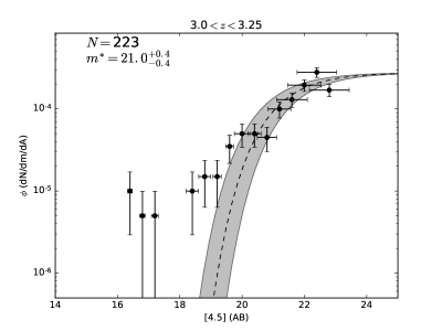
Figure 1.— The 4.5$\mu$m Luminosity Function of CCPC galaxies at redshifts $3.0\leq z<3.25$. $\phi$ is the number of galaxies at a specific magnitude per square arcminute ($dN/dm/dA$). Uncertainties in the number density of sources are Poissonian ($\sqrt{N(dm)}$), while the magnitude uncertainties in each bin are the average uncertainty of the bin’s galaxies. SciPy’s curvefit routine’s best fit to the data is the black dashed line. The number of galaxies in the plot and the value of $m^{*}$ and its $2\sigma$ bootstrapped uncertainties are listed in the top left corner. In this work, $\alpha$ is defined to be -1. The gray shaded area represents the 95% bootstrapped confidence region of the fit.

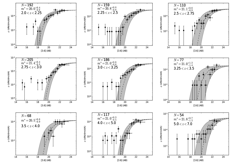
Figure 2.— The 3.6$\mu$m Spitzer Luminosity Function at nine epochs across $2\leq z<7$. The surface number density ($\phi$) of galaxies is measured in square arcminutes. The number density uncertainty is calculated by the root $N$ value in each bin, while the magnitude uncertainties are the average photometric errors in that bin. The gray shaded regions are the 95% confidence intervals calculated by bootstrapping. The Schechter fit (Eq 2) to the CCPC data is the black dashed line, with $\alpha$ defined as -1. The number of galaxies and the value of $m^{*}$ are listed in the upper left hand corner. The $m^{*}$ uncertainties are the bootstrapped $2\sigma$ values. Galaxies much brighter than $m^{*}$ we refer to as ‘hyperluminous’ sources and will be discussed in Section  LABEL:sec:dis.

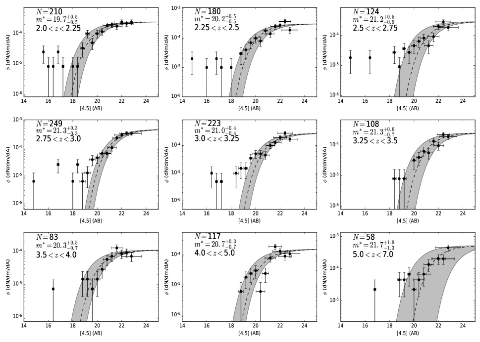
Figure 3.— The 4.5$\mu$m version of Figure  2.

Table 13.6$\mu$m CCPC Luminosity Function

$2\leq z<2.25$ & 192 20.01 ${}_{-0.65}^{+0.50}$ 2.94$\times 10^{-4}$
$2.25\leq z<2.5$ 159 20.89 ${}_{-0.68}^{+0.88}$ 3.41$\times 10^{-4}$
$2.5\leq z<2.75$ 110 21.13 ${}_{-0.96}^{+0.67}$ 3.39$\times 10^{-4}$
$2.75\leq z<3$ 205 21.42 ${}_{-0.33}^{+0.46}$ 5.01$\times 10^{-4}$
$3\leq z<3.25$ 186 21.06 ${}_{-0.65}^{+0.60}$ 2.74$\times 10^{-4}$
$3.25\leq z<3.5$ 77 21.07 ${}_{-1.47}^{+1.22}$ 2.05$\times 10^{-4}$
$3.5\leq z<4$ 68 20.51 ${}_{-0.99}^{+0.63}$ 1.34$\times 10^{-4}$
$4\leq z<5$ 117 21.06 ${}_{-0.49}^{+0.38}$ 1.75$\times 10^{-4}$
$5\leq z<6.6$ 54 21.83 ${}_{-1.23}^{+0.74}$ 6.30$\times 10^{-4}$

Note. — The results of fitting a Schechter function (Equation  2) to the CCPC galaxies in a series of redshift bins (1^st column). The number of galaxies ($N$) in each redshift bin is listed in the 2^nd column, followed by the fitted $m^{*}$ parameter in the 3^rd column. The 4^th column represents the 95$\%$ confidence interval of the $m^{*}$ value. This uncertainty was computed by bootstrapping with resampling of the data. The characteristic density ($\phi^{*}$) in units of the number of galaxies per magnitude bin per square arcminute is found in the final column. The faint end slope of the LF was fixed to be $\alpha=-1$.

Table 24.5$\mu$m CCPC Luminosity Function

Redshift	$N$	$m^{*}$	$2\sigma(m^{*})$	$\phi^{*}$
Range	Galaxies	(AB)	(95$\%$ CI)	(dN/dm/dA)
$2\leq z<2.25$	210	19.73	${}_{-0.59}^{+0.56}$	2.65$\times 10^{-4}$
$2.25\leq z<2.5$	180	20.27	${}_{-0.53}^{+0.56}$	3.35$\times 10^{-4}$
$2.5\leq z<2.75$	124	21.25	${}_{-0.97}^{+0.58}$	3.14$\times 10^{-4}$
$2.75\leq z<3$	249	21.36	${}_{-0.31}^{+0.39}$	5.13$\times 10^{-4}$
$3\leq z<3.25$	223	21.08	${}_{-0.46}^{+0.41}$	3.00$\times 10^{-4}$
$3.25\leq z<3.5$	108	21.31	${}_{-0.80}^{+0.71}$	2.76$\times 10^{-4}$
$3.5\leq z<4$	83	20.38	${}_{-0.74}^{+0.51}$	1.21$\times 10^{-4}$
$4\leq z<5$	117	20.71	${}_{-0.74}^{+0.35}$	1.68$\times 10^{-4}$
$5\leq z<6.6$	58	21.75	${}_{-1.38}^{+1.97}$

The spectroscopic redshifts used in the Field samples of galaxies (Section  3) came from the following sources (and references therein), as compiled by NED: 2008AnA...487..539W; 2004AJ....128..544M; 2004AnA...418..885N; 2005AnA...439..845L 2012ApJ...753...95B; 2010AnA...512A..12B; 2008ApJ...682..985W; 2009AnA...504..751S; 2004AnA...428.1043L 2012ApJS..203...15B; 2008ApJS..179...19L; 2008ApJS..179...95M; 2011ApJ...729...48B; 2011AJ....141...14S 2005AnA...437..883M; 2010ApJ...720..368X; 2011ApJ...743..144T; 2009ApJ...693.1713T; 2010MNRAS.405.2302H; 2009ApJ...706..885W 2013ApJ...772..113T; 2003MNRAS.344..169E; 2002AJ....124.1839B; 2009ApJ...699..667M; 2006ApJ...653.1004R 2006MNRAS.370.1185P; 2011MNRAS.413...80C; 2013ApJ...772...48P; 2006ApJ...646..107E; 2004ApJ...604..534S; 2001ApJ...559..620P 1999ApJ...513...34F; 2009ApJ...705...68B; 2001ApJS..135...41F; 2009ApJ...691..140H; 2009ApJ...697.1410L 2009AJ....137..179R; 2011ApJ...735...86W; 2010ApJ...717.1181P; 2012ApJ...759L..44G; 2013ApJ...776....9G; gob11 2009ApJ...690..295K; 2003ApJ...591..101E; 2005ApJ...626..698S; 2006ApJ...648..250C 2002AJ....123.3041K; 2003ApJ...592..728S; 2004AJ....127.2455A; 2002AnA...396..847V; 2007ApJ...655...51W; 2005ApJ...633.1126K 1998ApJ...499L.135S; 2013AnA...559A...2G; 2006AnA...457...79G; 2006AnA...450..495W; 2010ApJS..191..124S 2004ApJS..155..271S; 2010ApJ...722.1895E; 2013ApJ...765L...2B; 2014ApJ...793..101T; 2008ApJ...677..219K; 1999AnA...343..399W 2010AnA...509A..83D; 2010ApJ...716..348B; 2012MNRAS.423.2436S; 2014ApJ...791....3S 2002AnA...396..109P; 2004AnA...428..817K; 2000AnA...361L..25P; 2005AJ....130..867C; 2004AnA...428..793K; 1997AnA...326..505R 1997ApJ...481..673L; 2005ApJ...631..101P; 2002AJ....124.1886M; 2004ApJ...613..655W; 2011PASJ...63S.437T 2010ApJ...718..112Y; 2011MNRAS.416.2041M; 2005ApJ...620..595W; 2006MNRAS.371..221G; 2004ApJ...616...71S; 2010ApJ...715..385O 2004ApJ...612..108S; 1995AnA...294..377V; 2007ApJ...668...23P; 2004ApJ...614..671C; 2000AnA...362....9M 2000AJ....120.1648C; 2010MNRAS.401..294S; 2013AnA...557A..81M; 2014ApJ...788..125S; 2010ApJ...719.1393D; 2011MNRAS.411.2739C 2009AnA...501..865S; 2006AnA...449..951G; 2014MNRAS.440.3630R; 1994ApJ...436..678O 2005ApJ...618..123S; 1996ApJ...468..121S; 2004ApJ...606..664D; 2004AJ....127.3137C; 2004ApJ...612..122E; 2011ApJS..192....5A 2000AJ....119.2092B; 2009ApJ...703..198L; 1997ApJ...489..543P; 2008ApJS..179....1T; 2004ApJ...617...64S 2004AnA...424....1D; 1987ApJ...314..111A; 2010MNRAS.407..846D; 2011ApJ...740L..31E; 2012MNRAS.426.1073H 2009MNRAS.400..299L; 1999AnA...345...73P; 1997ApJ...478...87H; 1991MNRAS.250...24Y; 1995AJ....109.1522C 2004ApJS..155...73Z; 2014AJ....148...13R; 2011ApJ...735...87Y; 2007ApJ...660..167D; 2011AnA...526A..86G; 2004AJ....127.3121W 2006ApJ...637L...5D; 2012ApJ...745...33K; 2012ApJ...745...85L; 1996ApJ...457..102D; 1997ApJS..112....1T 1996AJ....112...62T; 2011ApJ...733...31H; 2001ApJ...560..127S; 2012ApJ...759..139K; 2009AnA...507.1277B; 2014ApJ...791...18B 2005ApJ...626..680D; 2005MNRAS.359..895V; 2008MNRAS.384.1611K; 2002AJ....123.1163B; 2001AJ....122..598D 1998AJ....115.1400F; 2003AJ....126.1183C; 2011ApJ...733L..11R; 2011MNRAS.412.1913I; 2006ApJ...647...74W; 2001AJ....121..662B 2001AJ....122.1125P; 1989AnA...218...71R; 2005AnA...440..881I; 2012AnA...537A..31C; 2011ApJ...736...48R 2007ApJ...659..941T; die13; 2013MNRAS.429.3047B; 1996Natur.381..759L; 1999ApJ...511L...1C; 2008MNRAS.389...45C 2000ApJ...545..591W; 2013MNRAS.430..425B; 2009ApJ...703.2033R; 2008ApJ...675..262R; 2005ApJ...629...72A 2012ApJS..199....3R; 2007ApJS..172...70L; 2002MNRAS.337.1153S; 2001AJ....122.2177B; 1995ApJ...448..575R; 2006ApJ...637..648S ven07; 1996ApJS..107...19M; 2007AnA...467...63T; 2004ApJ...606..683S; 2001AnA...380..409V 1998AJ....115.2184S; 2011ApJ...731...97S; 2004ApJ...611..732C; mag10; 2003AnA...407..147F; 2000ApJ...543..552S 2008AnA...492..637G; 2000AnA...359..489C; 2011ApJ...729L...4F; 2001ApJ...562...95S; 1995MNRAS.277..389R 2011ApJ...741...91C; 2001AnA...374..443F; 2001AnA...372L..57M; 2004AJ....127..131S; 2003ApJ...597..680W; 1997AnA...318..347S 1996ApJ...462...68S; 2005AnA...431..793V; 1996ApJ...471L..11L; 2008MNRAS.389.1223M; 2012ApJ...744..110C 2010ApJ...716L.200B; 2008AJ....135.1624S; 2007AJ....134..169X; 2009ApJ...691..687L; 2007ApJ...657..135C; 1998AJ....115...55L 2009ApJ...696.1195T; 2009AnA...497..689G; 2008ApJ...689..687B; 1998ApJ...494...60P; 2005ApJ...619..134T 2005ApJ...627...32S; 1993MNRAS.260..202H; 1995AnA...296..665V; 2011MNRAS.411.2336I; 2011ApJ...736...18N; 2006ApJ...651..688S 2004ApJ...606...85C; 2009MNRAS.396L...1W; 2004AJ....128.2073H; 2000ApJ...532..170S; 2004AnA...423..761V 1999ApJ...519....1S; 2002AnA...393..809M; 2001ApJ...549..770E; 1996AnA...305..450d; 2008AnA...492...81P; 2010MNRAS.401.1657L 2008AnA...483..415K; 2012AnA...537A..16F; 2006AnA...454..423V; 2014ApJ...793...92T; 2011AnA...528A..88G 2005AJ....130..496J; 2011ApJ...736...41B; 2001ApJ...554..742H; 2003AJ....126..632B; 2006ApJ...650..614H 2000ApJS..130...37S; 2000MNRAS.318..817S; 2008ApJS..176..301O; 2008AnA...478...83V 2007AnA...461...39F; 2009ApJ...698..740T; 2009ApJ...693....8B; 1992MNRAS.259p...1P; 2008ApJ...675.1076S 2011ApJ...738...69S; 2010ApJ...725.1011V; 2009ApJ...697..942R; 2009ApJ...695L.176D; 2004ApJ...611..660O 2006ApJ...653..988Y; 1994AnA...281..331S; 1991AJ....101.2004S; 2007MNRAS.376.1557I; 2006AnA...455..145T; 2009ApJ...706..762W 2004ApJ...617..707D; 2006MNRAS.372..357M; 2005ApJ...620L...1O; 2006ApJ...648...54S; 2009AnA...500L...1M 2010ApJ...725..394H; 2013AnA...555A..42R; 2013MNRAS.431.3589Z; 2009MNRAS.393.1174F; 2009ApJ...691..465F; 2010AnA...510A.109R 2007MNRAS.376..727S; 2005AnA...434...53V; 2010MNRAS.407L.103C; 2011ApJ...743..132P; 2004MNRAS.355..374B 2005ApJ...626..666M; 2005ApJ...621..582R; 2014AnA...564A.125B; 2008ApJ...673..686H; 2007MNRAS.376.1861F; 2004ApJ...604L..13S 2007ApJ...660...47D; 2011ApJ...735....5F; 2013MNRAS.432.2869H 2001AJ....121.1799P; 2003ApJ...596...67D; 2012ApJ...761..139C; 2009ApJ...701..915T; 2008ApJ...679..942M; 2012ApJ...744..149H 2007ApJS..172..523M; 2010MNRAS.408L..31D; 1996ApJ...459L..53H; 2013ApJ...763..120C; 1996ApJ...456L..13E 1996AnA...316...33W; 2006ApJ...650..604R; 2009ApJ...704..117K; 2013ApJ...763..129S; 2011ApJ...728L...2S; 2007ApJ...668..853K 1999PASP..111.1475S; 1998ApJ...505L..95W; 2002ApJ...570...92D; 2014AnA...562A..35N; 2002AstL...28....1R 1998AJ....116.2617S; 2004ApJ...610..635A; 2014AnA...569A..98T; 2011ApJ...734..119K; 2006PASJ...58..313S; 2014ApJ...792...15T 2013ApJ...772...99J; 2007AnA...468..877N; 2007ApJ...671.1227D; 2009ApJ...700...20L; 2001AJ....122..503A 2004AJ....127..563H; 1999ApJ...522L...9H; 2012MNRAS.422.1425C; 2010ApJ...723..869O; 2012AnA...547A..51G; 2009ApJ...696.1164O 2012ApJ...744..179S; 2012ApJ...744...83O; 2004ApJ...607..704S; 2011ApJ...743...65J; 2005PASJ...57..165T 2006ApJ...648....7K; 2006Natur.443..186I; 2004ApJ...613L...9N; 2005ApJ...634..142N; 2004ApJ...611...59R