Maximizing the Conditional Expected Reward for Reaching the Goal
(extended version)

Abstract

The paper addresses the problem of computing maximal conditional expected accumulated rewards until reaching a target state (briefly called maximal conditional expectations) in finite-state Markov decision processes where the condition is given as a reachability constraint. Conditional expectations of this type can, e.g., stand for the maximal expected termination time of probabilistic programs with non-determinism, under the condition that the program eventually terminates, or for the worst-case expected penalty to be paid, assuming that at least three deadlines are missed. The main results of the paper are (i) a polynomial-time algorithm to check the finiteness of maximal conditional expectations, (ii) PSPACE-completeness for the threshold problem in acyclic Markov decision processes where the task is to check whether the maximal conditional expectation exceeds a given threshold, (iii) an exponential-time algorithm for the threshold problem in the general (cyclic) case, and (iv) an exponential-time algorithm for computing the maximal conditional expectation and an optimal scheduler.

1 Introduction

Stochastic shortest (or longest) path problems are a prominent class of optimization problems where the task is to find a policy for traversing a probabilistic graph structure such that the expected value of the generated paths satisfying a certain objective is minimal (or maximal). In the classical setting (see e.g. [14, 33, 23, 28]), the underlying graph structure is given by a finite-state Markov decision process (MDP), i.e., a state-transition graph with nondeterministic choices between several actions for each of its non-terminal states, probability distributions specifying the probabilities for the successor states for each state-action pair and a reward function that assigns rational values to the state-action pairs. The stochastic shortest (longest) path problem asks to find a scheduler, i.e., a function that resolves the nondeterministic choices, possibly in a history-dependent way, which minimizes (maximizes) the expected accumulated reward until reaching a goal state. To ensure the existence of the expectation for given schedulers, one often assumes that the given MDP is contracting, i.e., the goal is reached almost surely under all schedulers, in which case the optimal expected accumulated reward is achieved by a memoryless deterministic scheduler that optimizes the expectation from each state and is computable using a linear program with one variable per state (see e.g. [28]). The contraction assumption can be relaxed by requiring the existence of at least one scheduler that reaches the goal almost surely and taking the extremum over all those schedulers [14, 23, 15]. These algorithms and corresponding value or policy iteration approaches have been implemented in various tools and used in many application areas.

The restriction to schedulers that reach the goal almost surely, however, limits the applicability and significance of the results. First, the known algorithms for computing extremal expected accumulated rewards are not applicable for models where the probability for never visiting a goal state is positive under each scheduler. Second, statements about the expected rewards for schedulers that reach the goal with probability 1 are not sufficient to draw any conclusion for the best- or worst-case behavior, if there exist schedulers that miss the goal with positive probability. This motivates the consideration of conditional stochastic path problems where the task is to compute the optimal expected accumulated reward until reaching a goal state, under the condition that a goal state will indeed be reached and where the extrema are taken over all schedulers that reach the goal with positive probability. More precisely, we address here a slightly more general problem where we are given two sets $F$ and $G$ of states in an MDP $\mathcal{M}$ with non-negative integer rewards and ask for the maximal expected accumulated reward until reaching $F$, under the condition that $G$ will be visited (denoted $\mathbb{E}^{\max}_{\mathcal{M},s_{\mathit{\scriptscriptstyle init}}}(\mathop{\raisebox{-1.07639pt}{\leavevmode\resizebox{6.24301pt}{}{\leavevmode\hbox{\set@color \leavevmode\hbox to12.69pt{\vbox to14.42pt{\text{[drawing]}}}}}}}\nolimits F|\Diamond G)$ where $s_{\mathit{\scriptscriptstyle init}}$ is the initial state of $\mathcal{M}$). Computation schemes for conditional expectations of this type can, e.g., be used to answer the following questions (assuming the underlying model is a finite-state MDP):

1. What is the maximal termination time of a probabilistic and nondeterministic program, under the condition that the program indeed terminates?

2. What are the maximal expected costs of the repair mechanisms that are triggered in cases where a specific failure scenario occurs, under the condition that the failure scenario indeed occurs?

3. What is the maximal energy consumption, under the condition that all jobs of a given list will be successfully executed within one hour?

The relevance of question (Q1) and related problems becomes clear from the work [24, 27, 29, 13, 19] on the semantics of probabilistic programs where no guarantees for almost-sure termination can be given. Question (Q2) is natural for a worst-case analysis of resilient systems or other types of systems where conditional probabilities serve to provide performance guarantees on the protocols triggered in exceptional cases that appear with positive, but low probability. Question (Q3) is typical when the task is to study the trade-off between cost and utility functions (see e.g. [9]). Given the work on anonymity and related notions for information leakage using conditional probabilities in MDP-like models [7, 20] or the formalization of posterior vulnerability as an expectation [4], the concept of conditional accumulated excepted rewards might also be useful to specify the degree of protection of secret data or to study the trade-off between privacy and utility, e.g., using gain functions [5, 3]. Other areas where conditional expectations play a crucial role are risk management where the conditional value-at-risk is used to formalize the expected loss under the assumption that very large losses occur [37, 2] or regression analysis where conditional expectations serve to predict the relation between random variables [35].

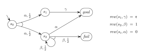
Figure 1: MDP $\mathcal{M}[\mathfrak{r}]$ for Example 1

Example 1

To illustrate the challenges for designing algorithms to compute maximal conditional expectations we regard the MDP $\mathcal{M}[\mathfrak{r}]$ shown in Figure 1. The reward of the state-action pair $(s_{1},\gamma)$ is given by a reward parameter $\mathfrak{r}\in\mathbb{N}$. Let $s_{\mathit{\scriptscriptstyle init}}=s_{0}$ be the initial state and $F=G=\{\mathit{goal}\}$. The only nondeterministic choice is in state $s_{2}$, while states $s_{0}$ and $s_{1}$ behave purely probabilistic and $\mathit{goal}$ and $\mathit{fail}$ are trap states. Given a scheduler $\mathfrak{S}$, we write $\mathbb{CE}^{\mathfrak{S}}$ for the conditional expectation $\mathbb{E}^{\mathfrak{S}}_{\mathcal{M}[\mathfrak{r}],s_{0}}(\mathop{\raisebox{-1.07639pt}{\leavevmode\resizebox{6.24301pt}{}{\leavevmode\hbox{\set@color \leavevmode\hbox to12.69pt{\vbox to14.42pt{\text{[drawing]}}}}}}}\nolimits\mathit{goal}|\Diamond\mathit{goal})$. (See also Section 2 for our notations.) For the two memoryless schedulers that choose $\alpha$ resp. $\beta$ in state $s_{2}$ we have:

$$\mathbb{CE}^{\alpha}\ \ =\ \ \frac{\frac{1}{2}\cdot\mathfrak{r}\ +\ \frac{1}{2}\cdot 0}{\frac{1}{2}+\frac{1}{2}}\ \ =\ \ \frac{\mathfrak{r}}{2}\ \ \ \ \ \text{and}\ \ \ \ \ \mathbb{CE}^{\beta}\ \ =\ \ \frac{\frac{1}{2}\cdot\mathfrak{r}\ +\ 0}{\frac{1}{2}+0}\ \ =\ \ \mathfrak{r}$$

We now regard the schedulers $\mathfrak{S}_{n}$ for $n=1,2,\ldots$ that choose $\beta$ for the first $n$ visits of $s_{2}$ and action $\alpha$ for the $(n{+}1)$-st visit of $s_{2}$. Then:

$$\mathbb{CE}^{\mathfrak{S}_{n}}\ \ =\ \ \frac{\frac{1}{2}\cdot\mathfrak{r}\ +\ \frac{1}{2}\cdot\frac{1}{2^{n}}\cdot n}{\frac{1}{2}\ +\ \frac{1}{2}\cdot\frac{1}{2^{n}}}\ \ =\ \ \mathfrak{r}\ +\ \frac{n-\mathfrak{r}}{2^{n}{+}1}$$

Thus, $\mathbb{CE}^{\mathfrak{S}_{n}}>\mathbb{CE}^{\beta}$ iff $n>\mathfrak{r}$, and the maximum is achieved for $n=\mathfrak{r}{+}2$.

This example illustrates three phenomena that distinguish conditional and unconditional expected accumulated rewards and make reasoning about maximal conditional expectations harder than about unconditional ones. First, optimal schedulers for $\mathcal{M}[\mathfrak{r}]$ need a counter for the number of visits in state $s_{2}$. Hence, memoryless schedulers are not powerful enough to maximize the conditional expectation. Second, while the maximal conditional expectation for $\mathcal{M}[\mathfrak{r}]$ with initial state $s_{\mathit{\scriptscriptstyle init}}=s_{0}$ is finite, the maximal conditional expectation for $\mathcal{M}[\mathfrak{r}]$ with starting state $s_{2}$ is infinite as:

$\sup\limits_{n\in\mathbb{N}}\ \mathbb{E}^{\mathfrak{S}_{n}}_{\mathcal{M}[\mathfrak{r}],s_{2}}(\mathop{\raisebox{-1.07639pt}{\leavevmode\resizebox{6.24301pt}{}{\leavevmode\hbox{\set@color \leavevmode\hbox to12.69pt{\vbox to14.42pt{\text{[drawing]}}}}}}}\nolimits\mathit{goal}|\Diamond\mathit{goal})\ \ =\ \ \sup\limits_{n\in\mathbb{N}}\frac{\ \frac{n}{2^{n}}\ }{\frac{1}{2^{n}}}\ \ =\ \ \infty$

Third, as $\mathfrak{S}_{2}$ maximizes the conditional expected accumulated reward for $\mathfrak{r}=0$, while $\mathfrak{S}_{3}$ is optimal for $\mathfrak{r}=1$, optimal decisions for paths ending in state $s_{2}$ depend on the reward value $r$ of the $\gamma$-transition from state $s_{1}$, although state $s_{1}$ is not reachable from $s_{2}$. Thus, optimal decisions for a path $\pi$ do not only depend on the past (given by $\pi$) and possible future (given by the sub-MDP that is reachable from $\pi$’s last state), but require global reasoning. ${\scriptscriptstyle\blacksquare}$

The main results of this paper are the following theorems. We write $\mathbb{CE}^{\max}$ for the maximal conditional expectation, i.e., the supremum of the conditional expectations $\mathbb{E}^{\mathfrak{S}}_{\mathcal{M},s_{\mathit{\scriptscriptstyle init}}}(\mathop{\raisebox{-1.07639pt}{\leavevmode\resizebox{6.24301pt}{}{\leavevmode\hbox{\set@color \leavevmode\hbox to12.69pt{\vbox to14.42pt{\text{[drawing]}}}}}}}\nolimits F|\Diamond G)$, when ranging over all schedulers $\mathfrak{S}$ where $\mathrm{Pr}^{\mathfrak{S}}_{\mathcal{M},s_{\mathit{\scriptscriptstyle init}}}(\Diamond G)$ is positive and $\mathrm{Pr}^{\mathfrak{S}}_{\mathcal{M},s_{\mathit{\scriptscriptstyle init}}}(\Diamond F|\Diamond G)=1$. (See also Section 2 for our notations.)

Theorem 1 (Checking finiteness and upper bound)

There is a polynomial-time algorithm that checks if $\mathbb{CE}^{\max}$ is finite. If so, an upper bound $\mathbb{CE}^{\mathrm{ub}}$ for $\mathbb{CE}^{\max}$ is computable in pseudo-polynomial time for the general case and in polynomial time if $F=G$ and $\mathrm{Pr}^{\min}_{\mathcal{M},s}(\Diamond G)>0$ for all states $s$ with $s\models\exists\Diamond G$.

The threshold problem asks whether the maximal conditional expectation exceeds or misses a given rational threshold $\vartheta$.

Theorem 2 (Threshold problem)

The problem “does $\mathbb{CE}^{\max}\bowtie\vartheta$ hold?” (where $\bowtie\ \in\{>,\geqslant,<,\leqslant\}$) is PSPACE-hard and solvable in exponential time. It is PSPACE-complete for acyclic MDPs.

For the computation of an optimal scheduler, we suggest an iterative scheduler-improvement algorithm that interleaves calls of the threshold algorithm with linear programming techniques to handle zero-reward actions. This yields:

Theorem 3 (Computing optimal schedulers)

The value $\mathbb{CE}^{\max}$ and an optimal scheduler $\mathfrak{S}$ are computable in exponential time.

Algorithms for checking finiteness and computing an upper bound (Theorem 1) will be sketched in Sections 3. Section 4 presents an exponential threshold algorithm and a polynomially space-bounded algorithm for acyclic MDPs (Theorem 2) as well as an exponential-time computation scheme for the construction of an optimal scheduler (Theorem 3). Further details, soundness proofs and a proof for the PSPACE-hardness as stated in Theorem 2 can be found in the appendix. The general feasibility of the algorithms will be shown by experimental studies with a prototypical implementation (for details, see Appendix 0.K).

Related work. Although conditional expectations appear rather naturally in many applications and despite the large amount of publications on variants of stochastic path problems and other forms of expectations in MDPs (see e.g. [17, 34]), we are not aware that they have been addressed in the context of MDPs. Computation schemes for extremal conditional probabilities $\mathrm{Pr}^{\max}(\varphi|\psi)$ or $\mathrm{Pr}^{\min}(\varphi|\psi)$ where both the objective $\varphi$ and the assumption $\psi$ are path properties specified in some temporal logic have been studied in [8, 6, 11]. For reachability properties $\varphi$ and $\psi$, the algorithm of [8, 6] has exponential time complexity, while the algorithm of [11] runs in polynomial time. Although the approach of [11] is not applicable for calculating maximal conditional expectations (see Appendix 0.B), it can be used to compute an upper bound for $\mathbb{CE}^{\max}$ (see Section 3). Conditional expected rewards in Markov chains can be computed using the rescaling technique of [11] for finite Markov chains or the approximation techniques of [18, 1] for certain classes of infinite-state Markov chains. The conditional weakest precondition operator of [29] yields a technique to compute conditional expected rewards for purely probabilistic programs (without non-determinism).

2 Preliminaries

We briefly summarize our notations used for Markov decision processes. Further details can be found in textbooks, see e.g. [33, 28] or Chapter 10 in [10].

A Markov decision process (MDP) is a tuple $\mathcal{M}=(S,\mathit{Act},P,s_{\mathit{\scriptscriptstyle init}},\mathit{rew})$ where $S$ is a finite set of states, $\mathit{Act}$ a finite set of actions, $s_{\mathit{\scriptscriptstyle init}}\in S$ the initial state, $P:S\times\mathit{Act}\times S\to[0,1]\cap\mathbb{Q}$ is the transition probability function and $\mathit{rew}:S\times\mathit{Act}\to\mathbb{N}$ the reward function. We require that $\sum_{s^{\prime}\in S}P(s,\alpha,s^{\prime})\in\{0,1\}$ for all $(s,\alpha)\in S\times\mathit{Act}$. We write $\mathit{Act}(s)$ for the set of actions that are enabled in $s$, i.e., $\alpha\in\mathit{Act}(s)$ iff $P(s,\alpha,\cdot)$ is not the null function. State $s$ is called a trap if $\mathit{Act}(s)=\varnothing$. The paths of $\mathcal{M}$ are finite or infinite sequences $s_{0}\,\alpha_{0}\,s_{1}\,\alpha_{1}\,s_{2}\,\alpha_{2}\ldots$ where states and actions alternate such that $P(s_{i},\alpha_{i},s_{i+1})>0$ for all $i\geqslant 0$. A path $\pi$ is called maximal if it is either infinite or finite and its last state is a trap. If $\pi=s_{0}\,\alpha_{0}\,s_{1}\,\alpha_{1}\,s_{2}\,\alpha_{2}\ldots\alpha_{k-1}\,s_{k}$ is finite then $\mathit{rew}(\pi)=\mathit{rew}(s_{0},\alpha_{0})+\mathit{rew}(s_{1},\alpha_{1})+\ldots+\mathit{rew}(s_{k-1},\alpha_{k-1})$ denotes the accumulated reward and $\mathit{first}(\pi)=s_{0}$, $\mathit{last}(\pi)=s_{k}$ its first resp. last state. The size of $\mathcal{M}$, denoted $\mathit{size}(\mathcal{M})$, is the sum of the number of states plus the total sum of the logarithmic lengths of the non-zero probability values $P(s,\alpha,s^{\prime})$ and the reward values $\mathit{rew}(s,\alpha)$.

An end component of $\mathcal{M}$ is a strongly connected sub-MDP. End components can be formalized as pairs $\mathcal{E}=(E,\mathfrak{A})$ where $E$ is a nonempty subset of $S$ and $\mathfrak{A}$ a function that assigns to each state $s\in E$ a nonempty subset of $\mathit{Act}(s)$ such that the graph induced by $\mathcal{E}$ is strongly connected.

A (randomized) scheduler for $\mathcal{M}$, often also called policy or adversary, is a function $\mathfrak{S}$ that assigns to each finite path $\pi$ where $\mathit{last}(\pi)$ is not a trap a probability distribution over $\mathit{Act}(\mathit{last}(\pi))$. $\mathfrak{S}$ is called memoryless if $\mathfrak{S}(\pi)=\mathfrak{S}(\pi^{\prime})$ for all finite paths $\pi$, $\pi^{\prime}$ with $\mathit{last}(\pi)=\mathit{last}(\pi^{\prime})$, in which case $\mathfrak{S}$ can be viewed as a function that assigns to each non-trap state $s$ a distribution over $\mathit{Act}(s)$. $\mathfrak{S}$ is called deterministic if $\mathfrak{S}(\pi)$ is a Dirac distribution for each path $\pi$, in which case $\mathfrak{S}$ can be viewed as a function that assigns an action to each finite path $\pi$ where $\mathit{last}(\pi)$ is not a trap. We write $\mathrm{Pr}^{\mathfrak{S}}_{\mathcal{M},s}$ or briefly $\mathrm{Pr}^{\mathfrak{S}}_{s}$ to denote the probability measure induced by $\mathfrak{S}$ and $s$. Given a measurable set $\psi$ of maximal paths, then $\mathrm{Pr}^{\min}_{\mathcal{M},s}(\psi)=\inf_{\mathfrak{S}}\mathrm{Pr}^{\mathfrak{S}}_{\mathcal{M},s}(\psi)$ and $\mathrm{Pr}^{\max}_{\mathcal{M},s}(\psi)=\sup_{\mathfrak{S}}\mathrm{Pr}^{\mathfrak{S}}_{\mathcal{M},s}(\psi)$. We will use LTL-like notations to specify measurable sets of maximal paths. For these it is well-known that optimal deterministic schedulers exists. If $\psi$ is a reachability condition then even optimal deterministic memoryless schedulers exist.

Let $\varnothing\not=F\subseteq S$. For a comparison operator $\bowtie\ \in\{=,>,\geqslant,<,\leqslant\}$ and $r\in\mathbb{N}$, $\Diamond^{\bowtie r}F$ denotes the event “reaching $F$ along some finite path $\pi$ with $\mathit{rew}(\pi)\bowtie r$”. The notation $\mathop{\raisebox{-1.07639pt}{\leavevmode\resizebox{6.24301pt}{}{\leavevmode\hbox{\set@color \leavevmode\hbox to12.69pt{\vbox to14.42pt{\text{[drawing]}}}}}}}\nolimits F$ will be used for the random variable that assigns to each maximal path $\varsigma$ in $\mathcal{M}$ the reward $\mathit{rew}(\pi)$ of the shortest prefix $\pi$ of $\varsigma$ where $\mathit{last}(\pi)\in F$. If $\varsigma\not\models\Diamond F$ then $(\mathop{\raisebox{-1.07639pt}{\leavevmode\resizebox{6.24301pt}{}{\leavevmode\hbox{\set@color \leavevmode\hbox to12.69pt{\vbox to14.42pt{\text{[drawing]}}}}}}}\nolimits F)(\varsigma)=\infty$. If $s\in S$ then $\mathbb{E}^{\mathfrak{S}}_{\mathcal{M},s}(\mathop{\raisebox{-1.07639pt}{\leavevmode\resizebox{6.24301pt}{}{\leavevmode\hbox{\set@color \leavevmode\hbox to12.69pt{\vbox to14.42pt{\text{[drawing]}}}}}}}\nolimits F)$ denotes the expectation of $\mathop{\raisebox{-1.07639pt}{\leavevmode\resizebox{6.24301pt}{}{\leavevmode\hbox{\set@color \leavevmode\hbox to12.69pt{\vbox to14.42pt{\text{[drawing]}}}}}}}\nolimits F$ in $\mathcal{M}$ with starting state $s$ under $\mathfrak{S}$, which is infinite if $\mathrm{Pr}^{\mathfrak{S}}_{\mathcal{M},s}(\Diamond F)<1$. $\mathbb{E}^{\max}_{\mathcal{M},s}(\mathop{\raisebox{-1.07639pt}{\leavevmode\resizebox{6.24301pt}{}{\leavevmode\hbox{\set@color \leavevmode\hbox to12.69pt{\vbox to14.42pt{\text{[drawing]}}}}}}}\nolimits F)\in\mathbb{R}\cup\{\pm\infty\}$ stands for $\sup_{\mathfrak{S}}\mathbb{E}^{\mathfrak{S}}_{\mathcal{M},s}(\mathop{\raisebox{-1.07639pt}{\leavevmode\resizebox{6.24301pt}{}{\leavevmode\hbox{\set@color \leavevmode\hbox to12.69pt{\vbox to14.42pt{\text{[drawing]}}}}}}}\nolimits F)$ where the supremum is taken over all schedulers $\mathfrak{S}$ with $\mathrm{Pr}^{\mathfrak{S}}_{\mathcal{M},s}(\Diamond F)=1$. Let $\psi$ be a measurable set of maximal paths. $\mathbb{E}^{\mathfrak{S}}_{\mathcal{M},s}(\mathop{\raisebox{-1.07639pt}{\leavevmode\resizebox{6.24301pt}{}{\leavevmode\hbox{\set@color \leavevmode\hbox to12.69pt{\vbox to14.42pt{\text{[drawing]}}}}}}}\nolimits F|\psi)$ stands for the expectation of $\mathop{\raisebox{-1.07639pt}{\leavevmode\resizebox{6.24301pt}{}{\leavevmode\hbox{\set@color \leavevmode\hbox to12.69pt{\vbox to14.42pt{\text{[drawing]}}}}}}}\nolimits F$ w.r.t. the conditional probability measure $\mathrm{Pr}^{\mathfrak{S}}_{\mathcal{M},s}(\ \cdot\ |\psi)$ given by $\mathrm{Pr}^{\mathfrak{S}}_{\mathcal{M},s}(\varphi|\psi)=\mathrm{Pr}^{\mathfrak{S}}_{\mathcal{M},s}(\varphi\wedge\psi)/\mathrm{Pr}^{\mathfrak{S}}_{\mathcal{M},s}(\psi)$. $\mathbb{E}^{\max}_{\mathcal{M},s}(\mathop{\raisebox{-1.07639pt}{\leavevmode\resizebox{6.24301pt}{}{\leavevmode\hbox{\set@color \leavevmode\hbox to12.69pt{\vbox to14.42pt{\text{[drawing]}}}}}}}\nolimits F|\psi)$ is the supremum of $\mathbb{E}^{\mathfrak{S}}_{\mathcal{M},s}(\mathop{\raisebox{-1.07639pt}{\leavevmode\resizebox{6.24301pt}{}{\leavevmode\hbox{\set@color \leavevmode\hbox to12.69pt{\vbox to14.42pt{\text{[drawing]}}}}}}}\nolimits F|\psi)$ where $\mathrm{Pr}^{\mathfrak{S}}_{\mathcal{M},s}(\psi)>0$ and $\mathrm{Pr}^{\mathfrak{S}}_{\mathcal{M},s}(\Diamond F|\psi)=1$, and $\mathrm{Pr}^{\max}_{\mathcal{M},s}(\varphi|\psi)=\sup_{\mathfrak{S}}\mathrm{Pr}^{\mathfrak{S}}_{\mathcal{M},s}(\varphi|\psi)$ where $\mathfrak{S}$ ranges over all schedulers with $\mathrm{Pr}^{\mathfrak{S}}_{\mathcal{M},s}(\psi)>0$ and $\sup\varnothing=-\infty$.

For the remainder of this paper, we suppose that two nonempty subsets $F$ and $G$ of $S$ are given such that $\mathrm{Pr}^{\max}_{\mathcal{M},s}(\Diamond F|\Diamond G)=1$. The task addressed in this paper is to compute the maximal conditional expectation given by:

$\mathbb{CE}^{\max}_{\mathcal{M},s}\ \stackrel{{\scriptstyle\text{\tiny def}}}{{=}}\ \sup\limits_{\mathfrak{S}}\ \mathbb{CE}^{\mathfrak{S}}_{\mathcal{M},s}\in\mathbb{R}\cup\{\infty\}$  where  $\mathbb{CE}^{\mathfrak{S}}_{\mathcal{M},s}\ =\ \mathbb{E}^{\mathfrak{S}}_{\mathcal{M},s}(\mathop{\raisebox{-1.07639pt}{\leavevmode\resizebox{6.24301pt}{}{\leavevmode\hbox{\set@color \leavevmode\hbox to12.69pt{\vbox to14.42pt{\text{[drawing]}}}}}}}\nolimits F|\Diamond G)$

Here, $\mathfrak{S}$ ranges over all schedulers $\mathfrak{S}$ with $\mathrm{Pr}^{\mathfrak{S}}_{\mathcal{M},s}(\Diamond G)>0$ and $\mathrm{Pr}^{\mathfrak{S}}_{\mathcal{M},s}(\Diamond F|\Diamond G)=1$. If $\mathcal{M}$ and its initial state are clear from the context, we often simply write $\mathbb{CE}^{\max}$ resp. $\mathbb{CE}^{\mathfrak{S}}$. We assume that all states in $\mathcal{M}$ are reachable from $s_{\mathit{\scriptscriptstyle init}}$ and $s_{\mathit{\scriptscriptstyle init}}\notin F\cup G$ (as $\mathbb{CE}^{\max}=0$ if $s\in F$ and $\mathbb{CE}^{\max}=\mathbb{E}^{\max}_{\mathcal{M},s_{\mathit{\scriptscriptstyle init}}}(\mathop{\raisebox{-1.07639pt}{\leavevmode\resizebox{6.24301pt}{}{\leavevmode\hbox{\set@color \leavevmode\hbox to12.69pt{\vbox to14.42pt{\text{[drawing]}}}}}}}\nolimits F)$ if $s\in G\setminus F$).

3 Finiteness and upper bound

Checking finiteness. We sketch a polynomially time-bounded algorithm that takes as input an MDP $\mathcal{M}=(S,\mathit{Act},P,s_{\mathit{\scriptscriptstyle init}},\mathit{rew})$ with two distinguished subsets $F$ and $G$ of $S$ such that $\mathrm{Pr}^{\max}_{\mathcal{M},s_{\mathit{\scriptscriptstyle init}}}(\Diamond F|\Diamond G)=1$. If $\mathbb{CE}^{\max}=\mathbb{E}^{\max}_{\mathcal{M},s_{\mathit{\scriptscriptstyle init}}}(\mathop{\raisebox{-1.07639pt}{\leavevmode\resizebox{6.24301pt}{}{\leavevmode\hbox{\set@color \leavevmode\hbox to12.69pt{\vbox to14.42pt{\text{[drawing]}}}}}}}\nolimits F|\Diamond G)=\infty$ then the output is “no”. Otherwise, the output is an MDP $\hat{\mathcal{M}}=(\hat{S},\hat{\mathit{Act}},\hat{P},\hat{s}_{\mathit{\scriptscriptstyle init}},\hat{\mathit{rew}})$ with two trap states $\mathit{goal}$ and $\mathit{fail}$ such that:

1. $\mathbb{E}^{\max}_{\mathcal{M},s_{\mathit{\scriptscriptstyle init}}}(\mathop{\raisebox{-1.07639pt}{\leavevmode\resizebox{6.24301pt}{}{\leavevmode\hbox{\set@color \leavevmode\hbox to12.69pt{\vbox to14.42pt{\text{[drawing]}}}}}}}\nolimits F|\Diamond G)\ \ =\ \ \mathbb{E}^{\max}_{\hat{\mathcal{M}},\hat{s}_{\mathit{\scriptscriptstyle init}}}(\mathop{\raisebox{-1.07639pt}{\leavevmode\resizebox{6.24301pt}{}{\leavevmode\hbox{\set@color \leavevmode\hbox to12.69pt{\vbox to14.42pt{\text{[drawing]}}}}}}}\nolimits\mathit{goal}|\Diamond\mathit{goal})$,

2. $\hat{s}\models\exists\Diamond\mathit{goal}$ and $\mathrm{Pr}^{\min}_{\hat{\mathcal{M}},\hat{s}}\bigl{(}\Diamond(\mathit{goal}\vee\mathit{fail})\bigr{)}=1$ for all states $\hat{s}\in\hat{S}\setminus\{\mathit{fail}\}$, and

3. $\hat{\mathcal{M}}$ does not have critical schedulers where a scheduler $\mathfrak{U}$ for $\hat{\mathcal{M}}$ is said to be critical iff $\mathrm{Pr}^{\mathfrak{U}}_{\hat{\mathcal{M}},\hat{s}_{\mathit{\scriptscriptstyle init}}}(\Diamond\mathit{fail})=1$ and there is a reachable positive $\mathfrak{U}$-cycle.

We provide here the main ideas of the algorithms and refer to Appendix 0.C for the details. The algorithm first transforms $\mathcal{M}$ into an MDP $\tilde{\mathcal{M}}$ that permits to assume $F=G=\{\mathit{goal}\}$. Intuitively, $\tilde{\mathcal{M}}$ simulates $\mathcal{M}$, while operating in four modes: “normal mode”, “after $G$”, “after $F$” and “goal”. $\tilde{\mathcal{M}}$ starts in normal mode where it behaves as $\mathcal{M}$ as long as neither $F$ nor $G$ have been visited. If a $G\setminus F$-state has been reached in normal mode then $\tilde{\mathcal{M}}$ switches to the mode “after $G$”. Likewise, as soon as an $F\setminus G$-state has been reached in normal mode then $\tilde{\mathcal{M}}$ switches to the mode “after $F$”. $\tilde{\mathcal{M}}$ enters the goal mode (consisting of a single trap state $\mathit{goal}$) as soon as a path fragment containing a state in $F$ and a state in $G$ has been generated. This is the case if $\mathcal{M}$ visits an $F$-state in mode “after $G$” or a $G$-state in mode “after $F$”, or a state in $F\cap G$ in the normal mode. The rewards in the normal mode and in mode “after $G$” are precisely as in $\mathcal{M}$, while the rewards are 0 in all other cases. We then remove all states $\tilde{s}$ in the “after $G$” mode with $\mathrm{Pr}^{\max}_{\tilde{\mathcal{M}},\tilde{s}}(\Diamond\mathit{goal})<1$, collapse all states $\tilde{s}$ in $\tilde{\mathcal{M}}$ with $\tilde{s}\not\models\exists\Diamond\mathit{goal}$ into a single trap state called $\mathit{fail}$ and add zero-reward transitions to $\mathit{fail}$ from all states $\tilde{s}$ that are not in the “after $G$” mode and $\mathrm{Pr}^{\max}_{\tilde{\mathcal{M}},\tilde{s}}(\Diamond\mathit{goal})=0$. Using techniques as in the unconditional case [23] we can check whether $\tilde{\mathcal{M}}$ has positive end components, i.e., end components with at least one state-action pair $(s,\alpha)$ with $\mathit{rew}(s,\alpha)>0$. If so, then $\mathbb{E}^{\max}_{\mathcal{M},s_{\mathit{\scriptscriptstyle init}}}(\mathop{\raisebox{-1.07639pt}{\leavevmode\resizebox{6.24301pt}{}{\leavevmode\hbox{\set@color \leavevmode\hbox to12.69pt{\vbox to14.42pt{\text{[drawing]}}}}}}}\nolimits F|\Diamond G)=\infty$. Otherwise, we collapse each maximal end component of $\tilde{\mathcal{M}}$ into a single state.

Let $\hat{\mathcal{M}}$ denote the resulting MDP. It satisfies (1) and (2). Property (3) holds iff $\mathbb{E}^{\max}_{\hat{\mathcal{M}},\hat{s}_{\mathit{\scriptscriptstyle init}}}(\mathop{\raisebox{-1.07639pt}{\leavevmode\resizebox{6.24301pt}{}{\leavevmode\hbox{\set@color \leavevmode\hbox to12.69pt{\vbox to14.42pt{\text{[drawing]}}}}}}}\nolimits\mathit{goal}|\Diamond\mathit{goal})<\infty$. This condition can be checked in polynomial time using a graph analysis in the sub-MDP of $\hat{\mathcal{M}}$ consisting of the states $\hat{s}$ with $\mathrm{Pr}^{\min}_{\hat{\mathcal{M}},\hat{s}}(\Diamond\mathit{goal})=0$ (see Prop. 2 and Appendix 0.C.3).

Computing an upper bound. Due to the transformation used for checking finiteness of the maximal conditional expectation, we can now suppose that $\mathcal{M}=\hat{\mathcal{M}}$, $F=G=\{\mathit{goal}\}$ and that (2) and (3) hold. We now present a technique to compute an upper bound $\mathbb{CE}^{\mathrm{ub}}$ for $\mathbb{CE}^{\max}$. The upper bound will be used later to determine a saturation point from which on optimal schedulers behave memoryless (see Section 4).

We consider the MDP $\mathcal{M}^{\prime}$ simulating $\mathcal{M}$, while operating in two modes. In its first mode, $\mathcal{M}^{\prime}$ attaches the reward accumulated so far to the states. More precisely, the states of $\mathcal{M}^{\prime}$ in its first mode have the form $\langle s,r\rangle\in S\times\mathbb{N}$ where $0\leqslant r\leqslant R$ and $R=\sum_{s\in S^{\prime}}\max\{\mathit{rew}_{\mathcal{M}^{\prime}}(s,\alpha):\alpha\in\mathit{Act}_{\mathcal{M}^{\prime}}(s)\}$. The initial state of $\mathcal{M}^{\prime}$ is $s_{\mathit{\scriptscriptstyle init}}^{\prime}=\langle s_{\mathit{\scriptscriptstyle init}},0\rangle$. The reward for the state-action pairs $(\langle s,r\rangle,\alpha)$ where $r{+}\mathit{rew}(s,\alpha)\leqslant R$ is 0. If $\mathcal{M}^{\prime}$ fires an action $\alpha$ in state $\langle s,r\rangle$ where $r^{\prime}\stackrel{{\scriptstyle\text{\tiny def}}}{{=}}r{+}\mathit{rew}(s,\alpha)>R$ then it switches to the second mode, while earning reward $r^{\prime}$. In its second mode $\mathcal{M}^{\prime}$ behaves as $\mathcal{M}$ without additional annotations of the states and earning the same rewards as $\mathcal{M}$. From the states $\langle\mathit{goal},r\rangle$, $\mathcal{M}^{\prime}$ moves to $\mathit{goal}$ with probability 1 and reward $r$. There is a one-to-one correspondence between the schedulers for $\mathcal{M}$ and $\mathcal{M}^{\prime}$ and the switch from $\mathcal{M}$ to $\mathcal{M}^{\prime}$ does not affect the probabilities and the accumulated rewards until reaching $\mathit{goal}$.

Let $\mathcal{N}$ denote the MDP resulting from $\mathcal{M}^{\prime}$ by adding reset-transitions from $\mathit{fail}$ (as a state of the second mode) and the copies $\langle\mathit{fail},r\rangle$ in the first mode to the initial state $s_{\mathit{\scriptscriptstyle init}}^{\prime}$. The reward of all reset transitions is 0. The reset-mechanism has been taken from [11] where it has been introduced as a technique to compute maximal conditional probabilities for reachability properties. Intuitively, $\mathcal{N}$ “discards” all paths of $\mathcal{M}^{\prime}$ that eventually enter $\mathit{fail}$ and “redistributes” their probabilities to the paths that eventually enter the goal state. In this way, $\mathcal{N}$ mimics the conditional probability measures $\mathrm{Pr}^{\mathfrak{S}}_{\mathcal{M}^{\prime},s_{\mathit{\scriptscriptstyle init}}^{\prime}}(\ \cdot\ |\Diamond\mathit{goal})=\mathrm{Pr}^{\mathfrak{S}}_{\mathcal{M},s_{\mathit{\scriptscriptstyle init}}}(\ \cdot\ |\Diamond\mathit{goal})$ for prefix-independent path properties. Paths $\pi$ from $s_{\mathit{\scriptscriptstyle init}}$ to $\mathit{goal}$ in $\mathcal{M}$ are simulated in $\mathcal{N}$ by paths of the form $\varrho=\xi_{1};\ldots\xi_{k};\pi$ where $\xi_{i}$ is a cycle in $\mathcal{N}$ with $\mathit{first}(\xi_{i})=s_{\mathit{\scriptscriptstyle init}}^{\prime}$ and $\xi_{i}$’s last transition is a reset-transition from some fail-state to $s_{\mathit{\scriptscriptstyle init}}^{\prime}$. Thus, $\mathit{rew}(\pi)\leqslant\mathit{rew}_{\mathcal{N}}(\varrho)$. The distinction between the first and second mode together with property (3) ensure that the new reset-transitions do not generate positive end components in $\mathcal{N}$. By the results of [23], the maximal unconditional expected accumulated reward in $\mathcal{N}$ is finite and we have:

$\mathbb{E}^{\max}_{\mathcal{M},s_{\mathit{\scriptscriptstyle init}}}(\mathop{\raisebox{-1.07639pt}{\leavevmode\resizebox{6.24301pt}{}{\leavevmode\hbox{\set@color \leavevmode\hbox to12.69pt{\vbox to14.42pt{\text{[drawing]}}}}}}}\nolimits\mathit{goal}|\Diamond\mathit{goal})\ \ =\ \ \mathbb{E}^{\max}_{\mathcal{M}^{\prime},s_{\mathit{\scriptscriptstyle init}}^{\prime}}(\mathop{\raisebox{-1.07639pt}{\leavevmode\resizebox{6.24301pt}{}{\leavevmode\hbox{\set@color \leavevmode\hbox to12.69pt{\vbox to14.42pt{\text{[drawing]}}}}}}}\nolimits\mathit{goal}|\Diamond\mathit{goal})\ \ \leqslant\ \ \mathbb{E}^{\max}_{\mathcal{N},s_{\mathit{\scriptscriptstyle init}}^{\prime}}(\mathop{\raisebox{-1.07639pt}{\leavevmode\resizebox{6.24301pt}{}{\leavevmode\hbox{\set@color \leavevmode\hbox to12.69pt{\vbox to14.42pt{\text{[drawing]}}}}}}}\nolimits\mathit{goal})$

Hence, we can deal with $\mathbb{CE}^{\mathrm{ub}}=\mathrm{E}^{\max}_{\mathcal{N},s_{\mathit{\scriptscriptstyle init}}^{\prime}}(\mathop{\raisebox{-1.07639pt}{\leavevmode\resizebox{6.24301pt}{}{\leavevmode\hbox{\set@color \leavevmode\hbox to12.69pt{\vbox to14.42pt{\text{[drawing]}}}}}}}\nolimits\mathit{goal})$, which is computable in time polynomial in the size of $\mathcal{N}$ by the algorithm proposed in [23]. As $\mathit{size}(\mathcal{N})=\Theta(R\cdot\mathit{size}(\mathcal{M}))$ we obtain a pseudo-polynomial time bound for the general case. If, however, $\mathrm{Pr}^{\min}_{\mathcal{M},s}(\Diamond\mathit{goal})>0$ for all states $s\in S\setminus\{\mathit{fail}\}$ then there is no need for the detour via $\mathcal{M}^{\prime}$ and we can apply the reset-transformation $\mathcal{M}\leadsto\mathcal{N}$ by adding a reset-transition from $\mathit{fail}$ to $s_{\mathit{\scriptscriptstyle init}}$ with reward 0, in which case the upper bound $\mathbb{CE}^{\mathrm{ub}}=\mathbb{E}^{\max}_{\mathcal{N},s_{\mathit{\scriptscriptstyle init}}}(\mathop{\raisebox{-1.07639pt}{\leavevmode\resizebox{6.24301pt}{}{\leavevmode\hbox{\set@color \leavevmode\hbox to12.69pt{\vbox to14.42pt{\text{[drawing]}}}}}}}\nolimits\mathit{goal})$ is obtained in time polynomial in the size of $\mathcal{M}$. For details we refer to the proof of Prop. 2 and Section 0.C.4 in the appendix.

4 Threshold algorithm and computing optimal schedulers

In what follows, we suppose that $\mathcal{M}=(S,\mathit{Act},P,s_{\mathit{\scriptscriptstyle init}},\mathit{rew})$ is an MDP with two trap states $\mathit{goal}$ and $\mathit{fail}$ such that $s\models\exists\Diamond\mathit{goal}$ for all states $s\in S\setminus\{\mathit{fail}\}$ and $\min_{s\in S}\mathrm{Pr}^{\min}_{\mathcal{M},s}(\Diamond(\mathit{goal}\vee\mathit{fail}))=1$ and $\mathbb{CE}^{\max}=\mathbb{E}^{\max}_{\mathcal{M},s_{\mathit{\scriptscriptstyle init}}}(\mathop{\raisebox{-1.07639pt}{\leavevmode\resizebox{6.24301pt}{}{\leavevmode\hbox{\set@color \leavevmode\hbox to12.69pt{\vbox to14.42pt{\text{[drawing]}}}}}}}\nolimits\mathit{goal}|\Diamond\mathit{goal})<\infty$.

A scheduler $\mathfrak{S}$ is said to be reward-based if $\mathfrak{S}(\pi)=\mathfrak{S}(\pi^{\prime})$ for all finite paths $\pi$, $\pi^{\prime}$ with $(\mathit{last}(\pi),\mathit{rew}(\pi))=(\mathit{last}(\pi^{\prime}),\mathit{rew}(\pi^{\prime}))$. Thus, deterministic reward-based schedulers can be seen as functions $\mathfrak{S}:S\times\mathbb{N}\to\mathit{Act}$. Prop. 3 in the appendix shows that $\mathbb{CE}^{\max}$ equals the supremum of the values $\mathbb{CE}^{\mathfrak{S}}$, when ranging over all deterministic reward-based schedulers $\mathfrak{S}$ with $\mathrm{Pr}^{\mathfrak{S}}_{\mathcal{M},s_{\mathit{\scriptscriptstyle init}}}(\Diamond\mathit{goal})>0$.

The basis of our algorithms are the following two observations. First, there exists a saturation point $\wp\in\mathbb{N}$ such that the optimal decision for all paths $\pi$ with $\mathit{rew}(\pi)\geqslant\wp$ is to maximize the probability for reaching the goal state (see Prop. 1 below). The second observation is a technical statement that will be used at several places. Let $\rho,\theta,\zeta,r,x,y,z,p\in\mathbb{R}$ with $0\leqslant p,x,y,z\leqslant 1$, $p>0$, $y>z$ and $x+z>0$ and let

$\mathsf{A}\ =\ \frac{\displaystyle\rho+p(ry+\theta)}{\displaystyle x+py}$,  $\mathsf{B}\ =\ \frac{\displaystyle\rho+p(rz+\zeta)}{\displaystyle x+pz}$  and  $\mathsf{C}=\max\{\mathsf{A},\mathsf{B}\}$

Then:

$$\mathsf{A}\geqslant\mathsf{B}\ \ \ \ \text{iff}\ \ \ \ r+\frac{\theta{-}\zeta}{y{-}z}\ \geqslant\ \mathsf{C}\ \ \ \ \text{iff}\ \ \ \ \theta-(\mathsf{C}{-}r)y\ \geqslant\ \zeta-(\mathsf{C}{-}r)z \dagger$$ ()

and the analogous statement for $>$ rather than $\geqslant$. This statement is a consequence of Lemma 16 in the appendix. We will apply this observation in different nuances. To give an idea how to apply statement ($\dagger$ ‣ 4), suppose $\mathsf{A}=\mathbb{CE}^{\mathfrak{T}}$ and $\mathsf{B}=\mathbb{CE}^{\mathfrak{U}}$ where $\mathfrak{T}$ and $\mathfrak{U}$ are reward-based schedulers that agree for all paths $\varrho$ that do not have a prefix $\pi$ with $\mathit{rew}(\pi)=r$ where $\mathit{last}(\pi)$ is a non-trap state, in which case $x$ denotes the probability for reaching $\mathit{goal}$ from $s_{\mathit{\scriptscriptstyle init}}$ along such a path $\varrho$ and $\rho$ stands for the corresponding partial expectation, while $p$ denotes the probability of the paths $\pi$ from $s_{\mathit{\scriptscriptstyle init}}$ to some non-trap state with $\mathit{rew}(\pi)=r$. The crucial observation is that $r+(\theta{-}\zeta)/(y{-}z)$ does not depend on $x,\rho,p$. Thus, if $r+(\theta{-}\zeta)/(y{-}z)\geqslant\mathbb{CE}^{\mathrm{ub}}$ for some upper bound $\mathbb{CE}^{\mathrm{ub}}$ of $\mathbb{CE}^{\max}$ then ($\dagger$ ‣ 4) allows to conclude that $\mathfrak{T}$’s decisions for the state-reward pairs $(s,r)$ are better than $\mathfrak{U}$, independent of $x,\rho$ and $p$.

Let $R\in\mathbb{N}$ and $\mathfrak{S}$, $\mathfrak{T}$ be reward-based schedulers. The residual scheduler $\mathfrak{S}{\uparrow}{R}$ is given by $(\mathfrak{S}{\uparrow}{R})(s,r)=\mathfrak{S}(s,R{+}r)$. $\mathfrak{S}\lhd_{R}\mathfrak{T}$ denotes the unique scheduler that agrees with $\mathfrak{S}$ for all state-reward pairs $(s,r)$ where $r<R$ and $(\mathfrak{S}\lhd_{R}\mathfrak{T}){\uparrow}{R}=\mathfrak{T}$. We write $\mathrm{E}^{\mathfrak{S}}_{\mathcal{M},s}$ for the partial expectation

$\mathrm{E}^{\mathfrak{S}}_{\mathcal{M},s}\ \ =\ \ \sum\limits_{r=0}^{\infty}\ \mathrm{Pr}^{\mathfrak{S}}_{\mathcal{M},s}(\Diamond^{=r}\mathit{goal})\cdot r$

Thus, $\mathrm{E}^{\mathfrak{T}}_{\mathcal{M},s}=\mathbb{E}^{\mathfrak{T}}_{\mathcal{M},s}(\mathop{\raisebox{-1.07639pt}{\leavevmode\resizebox{6.24301pt}{}{\leavevmode\hbox{\set@color \leavevmode\hbox to12.69pt{\vbox to14.42pt{\text{[drawing]}}}}}}}\nolimits\mathit{goal})$ if $\mathrm{Pr}^{\mathfrak{T}}_{\mathcal{M},s}(\Diamond\mathit{goal})=1$, while $\mathrm{E}^{\mathfrak{T}}_{\mathcal{M},s}<\infty=\mathbb{E}^{\mathfrak{T}}_{\mathcal{M},s}(\mathop{\raisebox{-1.07639pt}{\leavevmode\resizebox{6.24301pt}{}{\leavevmode\hbox{\set@color \leavevmode\hbox to12.69pt{\vbox to14.42pt{\text{[drawing]}}}}}}}\nolimits\mathit{goal})$ if $\mathrm{Pr}^{\mathfrak{T}}_{\mathcal{M},s}(\Diamond\mathit{goal})<1$.

Proposition 1

There exists a natural number $\wp$ (called saturation point of $\mathcal{M}$) and a deterministic memoryless scheduler $\mathfrak{M}$ such that:

1. $\mathbb{CE}^{\mathfrak{T}}\ \leqslant\ \mathbb{CE}^{\mathfrak{T}\lhd_{\wp}\mathfrak{M}}$ for each scheduler $\mathfrak{T}$ with $\mathrm{Pr}^{\mathfrak{T}}_{\mathcal{M},s_{\mathit{\scriptscriptstyle init}}}(\Diamond\mathit{goal})>0$, and

2. $\mathbb{CE}^{\mathfrak{S}}\ =\ \mathbb{CE}^{\max}$ for some deterministic reward-based scheduler $\mathfrak{S}$ such that $\mathrm{Pr}^{\mathfrak{S}}_{\mathcal{M},s_{\mathit{\scriptscriptstyle init}}}(\Diamond\mathit{goal})>0$ and $\mathfrak{S}{\uparrow}{\wp}=\mathfrak{M}$.

The proof of Prop. 1 (see Appendices 0.E and 0.F) is constructive and yields a polynomial-time algorithm for generating a scheduler $\mathfrak{M}$ as in Prop. 1 and a pseudo-polynomial algorithm for the computation of a saturation point $\wp$.

Scheduler $\mathfrak{M}$ maximizes the probability to reach $\mathit{goal}$ from each state. If there are two or more such schedulers, then $\mathfrak{M}$ is one where the conditional expected accumulated reward until reaching goal is maximal under all schedulers $\mathfrak{U}$ with $\mathrm{Pr}^{\mathfrak{U}}_{\mathcal{M},s}(\Diamond\mathit{goal})=\mathrm{Pr}^{\max}_{\mathcal{M},s}(\Diamond\mathit{goal})$ for all states $s$. Such a scheduler $\mathfrak{M}$ is computable in polynomial time using linear programming techniques. (See Lemma 10 in the appendix.)

The idea for the computation of the saturation point is to compute the threshold $\wp$ above which the scheduler $\mathfrak{M}$ becomes optimal. For this we rely on statement ($\dagger$ ‣ 4) where $\theta/y$ stands for the conditional expectation under $\mathfrak{M}$, $\zeta/z$ for the conditional expectation under an arbitrary scheduler $\mathfrak{S}$ and $\mathsf{C}=\mathbb{CE}^{\mathrm{ub}}$ is an upper bound of $\mathbb{CE}^{\max}$ (see Theorem 1), while $r=\wp$ is the wanted value. More precisely, for $s\in S$, let $\theta_{s}=\mathrm{E}^{\mathfrak{M}}_{\mathcal{M},s}$, $y_{s}=\mathrm{Pr}^{\mathfrak{M}}_{\mathcal{M},s}(\Diamond\mathit{goal})=\mathrm{Pr}^{\max}_{\mathcal{M},s}(\Diamond\mathit{goal})$. To compute a saturation point we determine the smallest value $\wp\in\mathbb{N}$ such that

$\theta_{s}-(\mathbb{CE}^{\mathrm{ub}}{-}\wp)\cdot y_{s}\ \ =\ \ \max\limits_{\mathfrak{S}}\ \bigl{(}\ \mathrm{E}^{\mathfrak{S}}_{\mathcal{M},s}-(\mathbb{CE}^{\mathrm{ub}}{-}\wp)\cdot\mathrm{Pr}^{\mathfrak{S}}_{\mathcal{M},s}(\Diamond\mathit{goal})\ \bigr{)}$

for all states $s$ where $\mathfrak{S}$ ranges over all schedulers for $\mathcal{M}$. In Appendix 0.F we show that instead of the maximum over all schedulers $\mathfrak{S}$ it suffices to take the local maximum over all “one-step-variants” of $\mathfrak{M}$. That is, a saturation point is obtained by $\wp=\max\{\lceil\mathbb{CE}^{\mathrm{ub}}-D\rceil,0\}$ where

$D\ =\ \min\ \bigl{\{}(\theta_{s}-\theta_{s,\alpha})/(y_{s}-y_{s,\alpha})\,:\,s\in S,\alpha\in\mathit{Act}(s),y_{s,\alpha}<y_{s}\bigr{\}}$

and $y_{s,\alpha}=\sum\limits_{t\in S}P(s,\alpha,t)\cdot y_{t}$ and $\theta_{s,\alpha}=\mathit{rew}(s,\alpha)\cdot y_{s,\alpha}+\sum\limits_{t\in S}P(s,\alpha,t)\cdot\theta_{t}$.

Example 2

The so obtained saturation point for the MDP $\mathcal{M}[\mathfrak{r}]$ in Figure 1 is $\wp=\lceil\mathbb{CE}^{\mathrm{ub}}{+}1\rceil$. Note that only state $s=s_{2}$ behaves nondeterministically, and $\mathfrak{M}(s)=\alpha$, $y_{s}=y_{s,\alpha}=1$, $\theta_{s}=\theta_{s,\alpha}=0$, while $y_{s,\beta}=\theta_{s,\beta}=\frac{1}{2}$. This yields $D=(0{-}\frac{1}{2})/(1{-}\frac{1}{2})=-1$. Thus, $\wp\geqslant\mathfrak{r}{+}2$ as $\mathbb{CE}^{\mathrm{ub}}\geqslant\mathbb{CE}^{\max}>\mathfrak{r}$. ${\scriptscriptstyle\blacksquare}$

The logarithmic length of $\wp$ is polynomial in the size of $\mathcal{M}$. Thus, the value (i.e., the length of an unary encoding) of $\wp$ can be exponential in $\mathit{size}(\mathcal{M})$. This is unavoidable as there are families $(\mathcal{M}_{k})_{k\in\mathbb{N}}$ of MDPs where the size of $\mathcal{M}_{k}$ is in $\mathcal{O}(k)$, while $2^{k}$ is a lower bound for the smallest saturation point of $\mathcal{M}_{k}$. This, for instance, applies to the MDPs $\mathcal{M}_{k}=\mathcal{M}[2^{k}]$ where $\mathcal{M}[\mathfrak{r}]$ is as in Figure 1. Recall from Example 1 that the scheduler $\mathfrak{S}_{\mathfrak{r}{+}2}$ that selects $\beta$ by the first $\mathfrak{r}{+}2$ visits of $s$ and $\alpha$ for the $(\mathfrak{r}{+}3)$-rd visit of $s$ is optimal for $\mathcal{M}[\mathfrak{r}]$. Hence, the smallest saturation point for $\mathcal{M}[2^{k}]$ is $2^{k}{+}2$.

Threshold algorithm. The input of the threshold algorithm is an MDP $\mathcal{M}$ as above and a non-negative rational number $\vartheta$. The task is to generate a deterministic reward-based scheduler $\mathfrak{S}$ with $\mathfrak{S}{\uparrow}{\wp}=\mathfrak{M}$ (where $\mathfrak{M}$ and $\wp$ are as in Prop. 1) such that $\mathbb{CE}^{\mathfrak{S}}>\vartheta$ if $\mathbb{CE}^{\max}>\vartheta$, and $\mathbb{CE}^{\mathfrak{S}}=\vartheta$ if $\mathbb{CE}^{\max}=\vartheta$. If $\mathbb{CE}^{\max}<\vartheta$ then the output of the threshold algorithm is “no”.

The algorithm operates level-wise and determines feasible actions $\mathit{action}(s,r)$ for all non-trap states $s$ and $r=\wp{-}1,\wp{-}2,\ldots,0$, using the decisions $\mathit{action}(\cdot,i)$ for the levels $i\in\{r{+}1,\ldots,\wp\}$ that have been treated before and linear programming techniques to treat zero-reward loops. In this context, feasibility is understood with respect to the following condition: If $\mathbb{CE}^{\max}\unrhd\vartheta$ where $\unrhd\in\{>,\geqslant\}$ then there exists a reward-based scheduler $\mathfrak{S}$ with $\mathbb{CE}^{\mathfrak{S}}\unrhd\vartheta$ and $\mathfrak{S}(s,R)=\mathit{action}(s,\min\{\wp,R\})$ for all $R\geqslant r$.

The algorithm stores for each state-reward pair $(s,r)$ the probabilities $y_{s,r}$ to reach $\mathit{goal}$ from $s$ and the corresponding partial expectation $\theta_{s,r}$ for the scheduler given by the decisions in the action table. The values for $r=\wp$ are given by $\mathit{action}(s,\wp)=\mathfrak{M}(s)$, $y_{s,\wp}=\mathrm{Pr}^{\mathfrak{M}}_{\mathcal{M},s}(\Diamond\mathit{goal})$ and $\theta_{s,\wp}=\mathrm{E}^{\mathfrak{M}}_{\mathcal{M},s}$. The candidates for the decisions at level $r<\wp$ are given by the deterministic memoryless schedulers $\mathfrak{P}$ for $\mathcal{M}$. We write $\mathfrak{P}_{+}$ for the reward-based scheduler given by $\mathfrak{P}_{+}(s,0)=\mathfrak{P}(s)$ and $\mathfrak{P}_{+}(s,i)=\mathit{action}(s,\min\{\wp,r{+}i\})$ for $i\geqslant 1$. Let $y_{s,r,\mathfrak{P}}=\mathrm{Pr}^{\mathfrak{P}_{+}}_{\mathcal{M},s}(\Diamond\mathit{goal})$ and $\theta_{s,r,\mathfrak{P}}=\mathrm{E}^{\mathfrak{P}_{+}}_{\mathcal{M},s}$ be the corresponding partial expectation.

To determine feasible actions for level $r$, the threshold algorithm makes use of a variant of ($\dagger$ ‣ 4) stating that if $\theta-(\vartheta{-}r)y\geqslant\zeta-(\vartheta{-}r)z$ and $\mathsf{B}\unrhd\vartheta$ then $\mathsf{A}\unrhd\vartheta$, where $\mathsf{A}$ and $\mathsf{B}$ are as in ($\dagger$ ‣ 4) and the requirement $y>z$ is dropped. Thus, the aim of the threshold algorithm is to compute a deterministic memoryless scheduler $\mathfrak{P}^{*}$ for $\mathcal{M}$ such that the following condition (* ‣ 4) holds:

$$\theta_{s,r,\mathfrak{P}^{*}}-(\vartheta{-}r)\cdot y_{s,r,\mathfrak{P}^{*}}\ \ =\ \ \max\limits_{\mathfrak{P}}\ \bigl{(}\ \theta_{s,r,\mathfrak{P}}-(\vartheta{-}r)\cdot y_{s,r,\mathfrak{P}}\ \bigr{)}$$ (*)

Such a scheduler $\mathfrak{P}^{*}$ is computable in time polynomial in the size of $\mathcal{M}$ (without the explicit consideration of all schedulers $\mathfrak{P}$ and their extensions $\mathfrak{P}_{+}$) using the following linear program with one variable $x_{s}$ for each state. The objective is to minimize $\sum\limits_{s\in S}x_{s}$ subject to the following conditions:

(1)	If $s\in S\setminus\{\mathit{goal},\mathit{fail}\}$ then for each action $\alpha\in\mathit{Act}(s)$ with $\mathit{rew}(s,\alpha)=0$:
	$x_{s}\ \ \geqslant\ \ \sum\limits_{t\in S}P(s,\alpha,t)\cdot x_{t}$
(2)	If $s\in S\setminus\{\mathit{goal},\mathit{fail}\}$ then for each action $\alpha\in\mathit{Act}(s)$ with $\mathit{rew}(s,\alpha)>0$:
	$x_{s}\ \ \geqslant\ \ \sum\limits_{t\in S}P(s,\alpha,t)\cdot\bigl{(}\,\theta_{t,R}+\mathit{rew}(s,\alpha)\cdot y_{t,R}\,-\,(\vartheta{-}r)\cdot y_{t,R}\,\bigr{)}$
	where $R=\min\{\wp,r{+}\mathit{rew}(s,\alpha)\}$
(3)	For the trap states:   $x_{\mathit{goal}}=r-\vartheta$   and   $x_{\mathit{fail}}=0$

This linear program has a unique solution $(x_{s}^{*})_{s\in S}$. Let $\mathit{Act}^{*}(s)$ denote the set of actions $\alpha\in\mathit{Act}(s)$ such that the following constraints (E1) and (E2) hold:

(E1) $$\text{If $\mathit{rew}(s,\alpha)=0$ then:}\ \ x_{s}^{*}\ =\ \sum_{t\in S}P(s,\alpha,t)\cdot x_{t}^{*}$$

(E2) If $$\mathit{rew}(s,\alpha)>0 R\,=\,\min\,\bigl{\{}\,\wp,\,r{+}\mathit{rew}(s,\alpha)\,\bigr{\}}$$ and then:

$$\hskip 28.45274pt\ x_{s}^{*}\ =\ \sum_{t\in S}P(s,\alpha,t)\cdot\bigl{(}\theta_{t,R}+\mathit{rew}(s,\alpha)\cdot y_{t,R}\,-\,(\vartheta{-}r)\cdot y_{t,R}\bigr{)}$$

Let $\mathcal{M}^{*}=\mathcal{M}^{*}_{r,\vartheta}$ denote the MDP with state space $S$ induced by the state-action pairs $(s,\alpha)$ with $\alpha\in\mathit{Act}^{*}(s)$ where the positive-reward actions are redirected to the trap states. Formally, for $s,t\in S$, $\alpha\in\mathit{Act}^{*}(s)$ we let $P_{\mathcal{M}^{*}}(s,\alpha,t)=P(s,\alpha,t)$ if $\mathit{rew}(s,\alpha)=0$ and $P_{\mathcal{M}^{*}}(s,\alpha,\mathit{goal})=\sum_{t\in S}P(s,\alpha,t)\cdot y_{t,R}$ and $P_{\mathcal{M}^{*}}(s,\alpha,\mathit{fail})=1-P_{\mathcal{M}^{*}}(s,\alpha,\mathit{goal})$ if $\mathit{rew}(s,\alpha)>0$ and $R=\min\{\wp,r{+}\mathit{rew}(s,\alpha)\}$. The reward structure of $\mathcal{M}^{*}$ is irrelevant for our purposes.

A scheduler $\mathfrak{P}^{*}$ satisfying (* ‣ 4) is obtained by computing a memoryless deterministic scheduler for $\mathcal{M}^{*}$ with $\mathrm{Pr}^{\mathfrak{P}^{*}}_{\mathcal{M}^{*},s}(\Diamond\mathit{goal})=\mathrm{Pr}^{\max}_{\mathcal{M}^{*},s}(\Diamond\mathit{goal})$ for all states $s$. This scheduler $\mathfrak{P}^{*}$ indeed provides feasible decisions for level $r$, i.e., if $\mathbb{CE}^{\max}\unrhd\vartheta$ where $\unrhd\in\{>,\geqslant\}$ then there exists a reward-based scheduler $\mathfrak{S}$ with $\mathbb{CE}^{\mathfrak{S}}\unrhd\vartheta$, $\mathfrak{S}(s,r)=\mathfrak{P}^{*}(s)$ and $\mathfrak{S}(s,R)=\mathit{action}(s,\min\{\wp,R\})$ for all $R>r$.

The threshold algorithm then puts $\mathit{action}(s,r)=\mathfrak{P}^{*}(s)$ and computes the values $y_{s,r}$ and $\theta_{s,r}$ as follows. Let $T$ denote the set of states $s\in S\setminus\{\mathit{goal},\mathit{fail}\}$ where $\mathit{rew}(s,\mathfrak{P}^{*}(s))>0$. For $s\in T$, the values $y_{s,r}=y_{s,r,\mathfrak{P}^{*}}$ and $\theta_{s,r}=\theta_{s,r,\mathfrak{P}^{*}}$ can be derived directly from the results obtained for the previously treated levels $r{+}1,\ldots,\wp$ as we have:

$y_{s,r}=\sum\limits_{t\in S}P(s,\alpha,t)\cdot y_{t,R}$

and

$\theta_{s,r}=\mathit{rew}(s,\alpha)\cdot y_{s,r}+\sum\limits_{t\in S}P(s,\alpha,t)\cdot\theta_{t,R}$

where $\alpha=\mathfrak{P}^{*}(s)$ and $R=\min\{\wp,r{+}\mathit{rew}(s,\alpha)\}$. For the states $s\in S\setminus T$:

$y_{s,r}=\sum\limits_{t\in T}\mathrm{Pr}^{\mathfrak{P}^{*}}_{\mathcal{M},s}(\neg T\operatorname{\mathrm{U}}t)\cdot y_{t,r}$   and   $\theta_{s,r}=\sum\limits_{t\in T}\mathrm{Pr}^{\mathfrak{P}^{*}}_{\mathcal{M},s}(\neg T\operatorname{\mathrm{U}}t)\cdot\theta_{t,r}$

Having treated the last level $r=0$, the output of the algorithm is as follows. Let $\mathfrak{S}$ be the scheduler given by the action table $\mathit{action}(\cdot)$. For the conditional expectation we have $\mathbb{CE}^{\mathfrak{S}}=\theta_{s_{\mathit{\scriptscriptstyle init}},0}/y_{s_{\mathit{\scriptscriptstyle init}},0}$ if $y_{s_{\mathit{\scriptscriptstyle init}},0}>0$. If $y_{s_{\mathit{\scriptscriptstyle init}},0}=0$ or $\theta_{s_{\mathit{\scriptscriptstyle init}},0}/y_{s_{\mathit{\scriptscriptstyle init}},0}<\vartheta$ then the algorithm returns the answer “no”. Otherwise, the algorithm returns $\mathfrak{S}$, in which case $\mathbb{CE}^{\mathfrak{S}}>\vartheta$ or $\mathbb{CE}^{\mathfrak{S}}=\vartheta=\mathbb{CE}^{\max}$. Proofs for the soundness and the exponential time complexity are provided in Appendix 0.G.

Example 3

For the MDP $\mathcal{M}[\mathfrak{r}]$ in Example 1, scheduler $\mathfrak{M}$ selects action $\alpha$ for state $s=s_{2}$. Thus, $\mathit{action}(s,\wp)=\alpha$ for the computed saturation point $\wp\geqslant\mathfrak{r}{+}2$ (see Example 2). The threshold algorithm for each positive rational threshold $\vartheta$ computes for each level $r=\wp{-}1,\wp{-}2,\ldots,1,0$ where $\mathit{action}(s,r{+}1)=\alpha$, the value $x_{s}^{*}=\max\{r{-}\vartheta,\frac{1}{2}+\frac{1}{2}(r{-}\vartheta)\}$ and the action set $\mathit{Act}^{*}(s)=\{\alpha\}$ if $r>\vartheta{+}1$, $\mathit{Act}^{*}(s)=\{\alpha,\beta\}$ if $r=\vartheta{+}1$ and $\mathit{Act}^{*}(s)=\{\beta\}$ if $r<\vartheta{+}1$. Thus, if $n=\min\{\wp,\lceil\vartheta{+}1\rceil\}$ then $\mathit{action}(s,r)=\alpha$, $y_{s,r}=1$, $\theta_{s,r}=0$ for $r\in\{n,\ldots,\wp\}$, while $\mathit{action}(s,n{-}k)=\beta$, $y_{s,n{-}k}=1/2^{k}$, $\theta_{s,n{-}k}=k/2^{k}$ for $k=1,\ldots,n$. That is, the threshold algorithm computes the scheduler $\mathfrak{S}_{n}$ that selects $\beta$ for the first $n$ visits of $s$ and $\alpha$ for the $(n{+}1)$-st visit of $s$. Thus, if $\mathfrak{r}\leqslant\vartheta<\mathfrak{r}{+}1$ then $n=\mathfrak{r}{+}2$, in which case the computed scheduler $\mathfrak{S}_{n}$ is optimal (see Example 1). The returned answer depends on whether $\vartheta\leqslant\mathbb{CE}^{\max}$. If, for instance, $\vartheta=\frac{\mathfrak{r}}{2}$ and $\mathfrak{r}>0$ is even then the threshold algorithm returns the scheduler $\mathfrak{S}_{n}$ where $n=\frac{\mathfrak{r}}{2}{+}1$, whose conditional expectation is $\mathfrak{r}-(\frac{\mathfrak{r}}{2}{-}1)/(2^{\frac{\mathfrak{r}}{2}+1}{+}1)>\frac{\mathfrak{r}}{2}=\vartheta$. ${\scriptscriptstyle\blacksquare}$

MDPs without zero-reward cycles and acyclic MDPs. If $\mathcal{M}$ does not contain zero-reward cycles then there is no need for the linear program. Instead we can use a topological sorting of the states in the graph of the sub-MDP consisting of zero-reward actions and determine a scheduler $\mathfrak{P}^{*}$ satisfying (* ‣ 4) directly. For acyclic MDPs, there is even no need for a saturation point. We can explore $\mathcal{M}$ using a recursive procedure and determine feasible decisions for each reachable state-reward pair $(s,r)$ on the basis of (* ‣ 4). This yields a polynomially space-bounded algorithm to decide whether $\mathbb{CE}^{\max}\unrhd\vartheta$ in acyclic MDPs. (See Appendix 0.I.)

Construction of an optimal scheduler. Let $\mathit{ThresAlgo}[\vartheta]$ denote the scheduler that is generated by calling the threshold algorithm for the threshold value $\vartheta$. A simple approach is to apply the threshold algorithm iteratively:

1. let $\mathfrak{S}$ be the scheduler $\mathfrak{M}$ as in Proposition 1;

2. REPEAT  $\vartheta:=\mathbb{CE}^{\mathfrak{S}}$;  $\mathfrak{S}:=\mathit{ThresAlgo}[\vartheta]$   UNTIL $\vartheta=\mathbb{CE}^{\mathfrak{S}}$;

3. return $\vartheta$ and $\mathfrak{S}$

The above algorithm generates a sequence of deterministic reward-based schedulers that are memoryless from $\wp$ on with strictly increasing conditional expectations. The number of such schedulers is bounded by $\mathit{md}^{\wp}$ where $\mathit{md}$ denotes the number of memoryless deterministic schedulers for $\mathcal{M}$. Hence, the algorithm terminates and correctly returns $\mathbb{CE}^{\max}$ and an optimal scheduler. As $\mathit{md}$ can be exponential in the number of states, this simple algorithm has double-exponential time complexity.

To obtain a (single) exponential-time algorithm, we seek for better (larger, but still promising) threshold values than the conditional expectation of the current scheduler. We propose an algorithm that operates level-wise and freezes optimal decisions for levels $r=\wp,\wp{-}1,\wp{-}2,\ldots,1,0$. The algorithm maintains and successively improves a left-closed and right-open interval $I=[A,B[$ with $\mathbb{CE}^{\max}\in I$ and $\mathbb{CE}^{\mathfrak{S}}\in I$ for the current scheduler $\mathfrak{S}$.

Initialization. The algorithm starts with the scheduler $\mathfrak{S}=\mathit{ThresAlgo}[\mathbb{CE}^{\mathfrak{M}}]$ where $\mathfrak{M}$ is as above. If $\mathbb{CE}^{\mathfrak{S}}=\mathbb{CE}^{\mathfrak{M}}$ then the algorithm immediately terminates. Suppose now that $\mathbb{CE}^{\mathfrak{S}}>\mathbb{CE}^{\mathfrak{M}}$. The initial interval is $I=[A,B[$ where $A=\mathbb{CE}^{\mathfrak{S}}$ and $B=\mathbb{CE}^{\mathrm{ub}}{+}1$ where $\mathbb{CE}^{\mathrm{ub}}$ is as in Theorem 1.

Level-wise scheduler improvement. The algorithm successively determines optimal decisions for the levels $r=\wp{-}1,\wp{-}2,\ldots,1,0$. The treatment of level $r$ consists of a sequence of scheduler-improvement steps where at the same time the interval $I$ is replaced with proper sub-intervals. The current scheduler $\mathfrak{S}$ has been obtained by the last successful run of the threshold algorithm, i.e., it has the form $\mathfrak{S}=\mathit{ThresAlgo}[\vartheta]$ where $\mathbb{CE}^{\mathfrak{S}}>\vartheta$. Besides the decisions of $\mathfrak{S}$ (i.e., the actions $\mathfrak{S}(s,R)$ for all state-reward pairs $(s,R)$ where $s\in S\setminus\{\mathit{goal},\mathit{fail}\}$ and $R\in\{0,1,\ldots,\wp\}$), the algorithm also stores the values $y_{s,R}$ and $\theta_{s,R}$ that have been computed in the threshold algorithm. For the current level $r$, the algorithm also computes for each state $s\in S\setminus\{\mathit{goal},\mathit{fail}\}$ and each action $\alpha\in\mathit{Act}(s)$ the values $y_{s,r,\alpha}=\sum_{t\in S}P(s,\alpha,t)\cdot y_{t,R}$ and $\theta_{s,r,\alpha}=\mathit{rew}(s,\alpha)\cdot y_{s,r,\alpha}\ +\ \sum_{t\in S}P(s,\alpha,t)\cdot\theta_{t,R}$ where $R=\min\{\wp,r+\mathit{rew}(s,\alpha)\}$.

Scheduler-improvement step. Let $r$ be the current level, $I=[A,B[$ the current interval and $\mathfrak{S}$ the current scheduler with $\mathbb{CE}^{\max}\in I$. At the beginning of the scheduler-improvement step we have $\mathbb{CE}^{\mathfrak{S}}=A$. Let

$$\begin{array}[]{rcl}\mathcal{I}_{\mathfrak{S},r}&\ =&\Bigl{\{}\ r+\frac{\theta_{s,r}-\theta_{s,r,\alpha}}{y_{s,r}-y_{s,r,\alpha}}\ :\ s\in S\setminus\{\mathit{goal},\mathit{fail}\},\ \alpha\in\mathit{Act}(s),\ y_{s,r}>y_{s,r,\alpha}\ \Bigr{\}}\\ \\[-4.30554pt] \mathcal{I}^{\uparrow}_{\mathfrak{S},r}&=&\bigl{\{}\ d\in\mathcal{I}_{\mathfrak{S},r}\ :\ d\ \geqslant\ \mathbb{CE}^{\mathfrak{S}}\bigr{\}}\hskip 28.45274pt\mathcal{I}^{B}_{\mathfrak{S},r}\ \ =\ \ \bigl{\{}\ d\in\mathcal{I}_{\mathfrak{S},r}\ :\ d<B\ \bigr{\}}\end{array}$$

Intuitively, the values in $d\in\mathcal{I}^{B}_{\mathfrak{S},r}$ are the “most promising” threshold values, as according to statement ($\dagger$ ‣ 4) these are the points where the decision of the current scheduler $\mathfrak{S}$ for some state-reward pair $(s,r)$ can be improved, provided that $\mathbb{CE}^{\max}>d$. (Note that the values in $\mathcal{I}_{\mathfrak{S},r}\setminus\mathcal{I}^{B}_{\mathfrak{S},r}$ can be discarded as $\mathbb{CE}^{\max}<B$.)

The algorithm proceeds as follows. If $\mathcal{I}^{B}_{\mathfrak{S},r}=\varnothing$ then no further improvements at level $r$ are possible as the function $\mathfrak{P}^{*}=\mathfrak{S}(\cdot,r)$ satisfies (* ‣ 4) for the (still unknown) value $\vartheta=\mathbb{CE}^{\max}$. See Lemma 25 in the appendix. In this case:

• If $r=0$ then the algorithm terminates with the answer $\mathbb{CE}^{\max}=\mathbb{CE}^{\mathfrak{S}}$ and $\mathfrak{S}$ as an optimal scheduler.

• If $r>0$ then the algorithm goes to the next level $r{-}1$ and performs the scheduler-improvement step for $\mathfrak{S}$ at level $r{-}1$.

Suppose now that $\mathcal{I}^{B}_{\mathfrak{S},r}$ is nonempty. Let $\mathcal{K}=\mathcal{I}^{\uparrow}_{\mathfrak{S},r}\cup\{\mathbb{CE}^{\mathfrak{S}}\}$. The algorithm seeks for the largest value $\vartheta^{\prime}\in\mathcal{K}\cap I$ such that $\mathbb{CE}^{\max}\geqslant\vartheta^{\prime}$. More precisely, it successively calls the threshold algorithm for the threshold value $\vartheta^{\prime}=\max(\mathcal{K}\cap I)$ and performs the following steps for the generated scheduler $\mathfrak{S}^{\prime}=\mathit{ThresAlgo}[\vartheta^{\prime}]$:

• If the result of the threshold algorithm is “no” and $\mathrm{Pr}^{\mathfrak{S}^{\prime}}_{\mathcal{M},s_{\mathit{\scriptscriptstyle init}}}(\Diamond\mathit{goal})$ is positive (in which case $\mathbb{CE}^{\mathfrak{S}^{\prime}}\leqslant\mathbb{CE}^{\max}<\vartheta^{\prime}$), then:

  • If $\mathbb{CE}^{\mathfrak{S}^{\prime}}\leqslant A$ then the algorithm refines $I$ by putting $B:=\vartheta^{\prime}$.

  • If $\mathbb{CE}^{\mathfrak{S}^{\prime}}>A$ then the algorithm refines $I$ by putting $A:=\mathbb{CE}^{\mathfrak{S}^{\prime}}$, $B:=\vartheta^{\prime}$ and adds $\mathbb{CE}^{\mathfrak{S}^{\prime}}$ to $\mathcal{K}$ (Note that then $\mathbb{CE}^{\mathfrak{S}^{\prime}}\in\mathcal{K}\cap I$, while $\mathbb{CE}^{\mathfrak{S}}\in\mathcal{K}\setminus I$.)

• Suppose now that $\mathbb{CE}^{\mathfrak{S}^{\prime}}\geqslant\vartheta^{\prime}$. The algorithm terminates if $\mathbb{CE}^{\mathfrak{S}^{\prime}}=\vartheta^{\prime}$, in which case $\mathfrak{S}^{\prime}$ is optimal. Otherwise, i.e., if $\mathbb{CE}^{\mathfrak{S}^{\prime}}>\vartheta^{\prime}$, then the algorithm aborts the loop by putting $\mathcal{K}:=\varnothing$, refines the interval $I$ by putting $A:=\mathbb{CE}^{\mathfrak{S}^{\prime}}$, updates the current scheduler by setting $\mathfrak{S}:=\mathfrak{S}^{\prime}$ and performs the next scheduler-improvement step.

The soundness proof and complexity analysis can be found in Appendix 0.H, where (among others) we show that the scheduler-improvement step for schedulers $\mathfrak{S}$ with $\mathbb{CE}^{\mathfrak{S}}<\mathbb{CE}^{\max}$ terminates with some scheduler $\mathfrak{S}^{\prime}$ such that $\mathbb{CE}^{\mathfrak{S}}<\mathbb{CE}^{\mathfrak{S}^{\prime}}$. The total number of calls of the threshold algorithm is in $\mathcal{O}(\wp\cdot\mathit{md}\cdot|S|\cdot|\mathit{Act}|)$. This yields an exponential time bound as stated in Theorem 3.

Example 4

We regard again the MDP $\mathcal{M}[\mathfrak{r}]$ of Example 1 where we suppose $\mathfrak{r}$ is positive and even. The algorithm first computes $\mathbb{CE}^{\mathrm{ub}}$ (see Section 3), a saturation point $\wp\geqslant\mathfrak{r}{+}2$ (see Example 2), the scheduler $\mathfrak{M}$, its conditional expectation $\mathbb{CE}^{\mathfrak{M}}=\frac{\mathfrak{r}}{2}$ and the scheduler $\mathfrak{S}=\mathit{ThresAlgo}[\frac{\mathfrak{r}}{2}]$. The initial interval is $I=[A,B[$ where $A=\mathbb{CE}^{\mathfrak{S}}=\mathfrak{r}-(\frac{\mathfrak{r}}{2}{-}1)/(2^{\frac{\mathfrak{r}}{2}+1}{+}1)$ (see Example 3) and $B=\mathbb{CE}^{\mathrm{ub}}{+}1$. The scheduler improvement step for $\mathfrak{S}$ at levels $r=\wp{-}1,\ldots,\mathfrak{r}{+}1$ determines the set $\mathcal{I}_{\mathfrak{S},r}=\{r{-}1\}$ and calls the threshold algorithm for $\vartheta^{\prime}=r{-}1$. These calls are not successful for $r=\wp{-}1,\ldots,\mathfrak{r}{+}2$. That is, the scheduler $\mathfrak{S}$ remains unchanged and the upper bound $B$ is successively improved to $r{-}1$. At level $r=\mathfrak{r}{+}1$, the threshold algorithm is called for $\vartheta^{\prime}=\mathfrak{r}$, which yields the optimal scheduler $\mathfrak{S}^{\prime}=\mathit{ThresAlgo}[\vartheta^{\prime}]$ (see Example 3). ${\scriptscriptstyle\blacksquare}$

Implementation and experiments. We have implemented the algorithms presented in this paper as a prototypical extension of the model checker PRISM [30, 32] and carried out initial experiments to demonstrate the general feasibility of our approach (see https://wwwtcs.inf.tu-dresden.de/ALGI/PUB/TACAS17/ and Appendix 0.K for details).

5 Conclusion

Although the switch to conditional expectations appears rather natural to escape from the limitations of known solutions for unconditional extremal expected accumulated rewards, to the best of our knowledge computation schemes for conditional expected accumulated rewards have not been addressed before. Our results show that new techniques are needed to compute maximal conditional expectations, as optimal schedulers might need memory and local reasoning in terms of the past and possible future is not sufficient (Example 1). The key observations for our algorithms are the existence of a saturation point $\wp$ for the reward that has been accumulated so far, from which on optimal schedulers can behave memoryless, and a linear correlation between optimal decisions for all state-reward pairs $(s,r)$ of the same reward level $r$ (see (* ‣ 4) and the linear program used in the threshold algorithm). The difficulty to reason about conditional expectations is also reflected in the achieved complexity-theoretic results stating that all variants of the threshold problem lie between PSPACE and EXPTIME. While PSPACE-completeness has been established for acyclic MDPs (Appendix 0.I), the precise complexity for cyclic MDPs is still open. In contrast, optimal schedulers for unconditional expected accumulated rewards as well as for conditional reachability probabilities are computable in polynomial time [23, 11].

Using standard automata-based approaches, our method can easily be generalized to compute maximal conditional expected rewards for regular co-safety conditions (rather than reachability conditions $\Diamond G$) and/or where the accumulation of rewards is “controlled” by a deterministic finite automaton as in the logics considered in [16, 12] (rather than $\mathop{\raisebox{-1.07639pt}{\leavevmode\resizebox{6.24301pt}{}{\leavevmode\hbox{\set@color \leavevmode\hbox to12.69pt{\vbox to14.42pt{\text{[drawing]}}}}}}}\nolimits F$). In this paper, we restricted to MDPs with non-negative integer rewards. Non-negative rational rewards can be treated by multiplying all reward values with their least common multiple (Appendix 0.J.1). In the case of acyclic MDPs, our methods are even applicable if the MDP has negative and positive rational rewards (Appendix 0.J.2). By swapping the sign of all rewards, this yields a technique to compute minimal conditional expectations in acyclic MDPs. We expect that minimal conditional expectations in cyclic MDPs with non-negative rewards can be computed using similar algorithms as we suggested for maximal conditional expectations. This as well as MDPs with negative and positive rewards will be addressed in future work.

APPENDIX

Outline of the appendix.

• Appendix 0.A (Relevant notations for the appendix, page 0.A) explains the notations used in the appendix.

• Appendix 0.B (Extremal conditional probabilities, page 0.B) sketches the reset mechanism of [11] for computing maximal conditional probabilities (used in Section 3 to compute an upper bound $\mathbb{CE}^{\mathrm{ub}}$). It also provides an example illustrating why the reset method fails for conditional expectations.

• Appendix 0.C (Finiteness and upper bound, page 0.C) deals with determining finiteness and the computation of an upper bound (Theorem 1).

• Appendix 0.D (Deterministic reward-based schedulers are sufficient, page 0.D) shows that deterministic reward-based schedulers are sufficient for maximizing the conditional expectation in our setting.

• Appendix 0.E (Existence of a saturation point and optimal schedulers, page 0.E) provides the proof for Proposition 1.

• Appendix 0.F (Computing a saturation point, page 0.F) shows the correctness of the computation of a saturation point as described in Section 4.

• Appendix 0.G (Threshold algorithm, page 0.G) provides additional details for the threshold algorithm as well as the proof of the soundness proof and the exponential time bound as stated in Theorem 2.

• Appendix 0.H (Computing an optimal scheduler and the maximal conditional expectation, page 0.H) provides additional details for the scheduler improvement algorithm of Section 4 and the proof of Theorem 3.

• Appendix 0.I (PSPACE-completeness for acyclic MPDs, page 0.I) provides the PSPACE-completeness proof of the threshold problem in acyclic MDPs as stated in Theorem 2.

• Appendix 0.J (Rational and negative rewards, page 0.J) provides details for rational and negative rewards as mentioned in the conclusion.

• Appendix 0.K (Implementation and experiments, page 0.K) provides details on our prototypical implementation in PRISM and our experiments.

Appendix 0.A Relevant notations for the appendix

Notations for Markov decision processes. A Markov decision process (MDP) is a tuple $\mathcal{M}=(S,\mathit{Act},P,s_{\mathit{\scriptscriptstyle init}},\mathit{rew})$ where $S$ is a finite set of states, $\mathit{Act}$ a finite set of actions, $s_{\mathit{\scriptscriptstyle init}}\in S$ the initial state, $P:S\times\mathit{Act}\times S\to[0,1]\cap\mathbb{Q}$ is the transition probability function and $\mathit{rew}:S\times\mathit{Act}\to\mathbb{N}$ the reward function. We require that $P(s,\alpha,S)\in\{0,1\}$ for all $(s,\alpha)\in S\times\mathit{Act}$ where, for $F\subseteq S$, $P(s,\alpha,F)=\sum_{t\in F}P(s,\alpha,t)$. We write $\mathit{Act}(s)$ for the set of actions that are enabled in $s$, i.e., $\alpha\in\mathit{Act}(s)$ iff $P(s,\alpha,\cdot)$ is not the null function. State $s$ is called a trap if $\mathit{Act}(s)=\varnothing$.

The paths of $\mathcal{M}$ are finite or infinite sequences $s_{0}\,\alpha_{0}\,s_{1}\,\alpha_{1}\,s_{2}\,\alpha_{2}\ldots$ where states and actions alternate such that $P(s_{i},\alpha_{i},s_{i+1})>0$ for all $i\geqslant 0$. A path $\pi$ is called maximal if it is either infinite or finite and its last state is a trap. If $\pi=s_{0}\,\alpha_{0}\,s_{1}\,\alpha_{1}\,s_{2}\,\alpha_{2}\ldots\alpha_{k-1}\,s_{k}$ is finite then

• $\mathit{rew}(\pi)=\mathit{rew}(s_{0},\alpha_{0})+\mathit{rew}(s_{1},\alpha_{1})+\ldots+\mathit{rew}(s_{k-1},\alpha_{k-1})$ denotes the accumulated reward,

• $|\pi|=k$ its length (number of transitions),

• $\mathrm{prob}(\pi)=P(s_{0},\alpha_{0},s_{1})\cdot P(s_{1},\alpha_{1},s_{2})\cdot\ldots\cdot P(s_{k-1},\alpha_{k-1},s_{k})$ its probability,

• $\mathit{first}(\pi)=s_{0}$, $\mathit{last}(\pi)=s_{k}$ its first resp. last state.

The notation $\pi_{1};\pi_{2}$ is used to denote the concatenation of paths $\pi_{1}$ and $\pi_{2}$ with $\mathit{last}(\pi_{1})=\mathit{first}(\pi_{2})$, where $\pi_{1};\pi_{2}=\pi_{2}$ if $|\pi_{1}|=0$.

The size of $\mathcal{M}$, denoted $\mathit{size}(\mathcal{M})$, is the sum of the number of states plus the total sum of the logarithmic lengths of the non-zero probability values $P(s,\alpha,s^{\prime})$ and the reward values $\mathit{rew}(s,\alpha)$.

Scheduler. A (randomized) scheduler for $\mathcal{M}$, often also called policy or adversary, is a function $\mathfrak{S}$ that assigns to each finite path $\pi$ where $\mathit{last}(\pi)$ is not a trap a probability distribution over $\mathit{Act}(\mathit{last}(\pi))$. $\mathfrak{S}$ is called memoryless if $\mathfrak{S}(\pi)=\mathfrak{S}(\pi^{\prime})$ for all finite paths $\pi$, $\pi^{\prime}$ with $\mathit{last}(\pi)=\mathit{last}(\pi^{\prime})$, in which case $\mathfrak{S}$ can be viewed as a function that assigns to each non-trap state $s$ a distribution over $\mathit{Act}(s)$. $\mathfrak{S}$ is called deterministic if $\mathfrak{S}(\pi)$ is a Dirac distribution for each path $\pi$, in which case $\mathfrak{S}$ can be viewed as a function that assigns an action to each finite path $\pi$ where $\mathit{last}(\pi)$ is not a trap. Given a scheduler $\mathfrak{S}$, a $\mathfrak{S}$-path is any path that might arise when the nondeterministic choices in $\mathcal{M}$ are resolved using $\mathfrak{S}$. Thus, $\varsigma\,=\,s_{0}\,\alpha_{0}\,s_{1}\,\alpha_{1}\ldots$ is a $\mathfrak{S}$-path iff $\varsigma$ is a path and $\mathfrak{S}(s_{0}\,\alpha_{0}\,s_{1}\,\alpha_{1}\ldots\alpha_{k-1}\,s_{k})(\alpha_{k})>0$ for all $k\geqslant 0$. If $\pi$ is a finite $\mathfrak{S}$-path then $\mathfrak{S}{\uparrow}{\pi}$ denotes the residual scheduler “$\mathfrak{S}$ after $\pi$” given by:

$(\mathfrak{S}{\uparrow}{\pi})(\varrho)$  $=$  $\mathfrak{S}(\pi;\varrho)$   if $\varrho$ is a finite path with $\mathit{last}(\pi)=\mathit{first}(\varrho)$

The behavior of $\mathfrak{S}{\uparrow}{\pi}$ for paths not starting in $\mathit{last}(\pi)$ is irrelevant.

Let $\mathfrak{S}$ and $\mathfrak{U}$ be schedulers. If $\pi$ is a finite $\mathfrak{S}$-path $\pi$, then $\mathfrak{S}\lhd_{\pi}\mathfrak{U}$ denotes the unique scheduler $\mathfrak{T}$ with $\mathfrak{T}{\uparrow}{\pi}=\mathfrak{U}$ that behaves as $\mathfrak{S}$ for all paths $\varrho$ where $\pi$ is not a prefix of $\varrho$. That is:

$$(\mathfrak{S}\lhd_{\pi}\mathfrak{U})(\varrho)\ \ =\ \ \left\{\begin{array}[]{lcl}\mathfrak{S}(\varrho)&:&\text{if $\pi$ is not a prefix of $\varrho$}\\ \mathfrak{U}(\varrho^{\prime})&:&\text{if $\varrho=\pi;\varrho^{\prime}$}\end{array}\right.$$

where $\pi;s=\pi$. Hence, $(\mathfrak{S}\lhd_{\pi}\mathfrak{U})(\pi)=\mathfrak{U}(\mathit{last}(\pi))$. If $R\in\mathbb{N}$ then $\mathfrak{S}\lhd_{R}\mathfrak{U}$ denotes the scheduler given by $(\mathfrak{S}\lhd_{R}\mathfrak{U})(\varrho)=\mathfrak{S}(\varrho)$ if $\mathit{rew}(\varrho)<R$ and $(\mathfrak{S}\lhd_{R}\mathfrak{U})(\pi;\varrho^{\prime})=\mathfrak{U}(\varrho^{\prime})$ if $\mathit{rew}(\pi)\geqslant R$ and $\mathit{rew}(\pi^{\prime})<R$ for all proper prefixes $\pi^{\prime}$ of $\pi$.

Scheduler $\mathfrak{S}$ is said to be reward-based if $\mathfrak{S}(\pi)=\mathfrak{S}(\pi^{\prime})$ for all finite paths $\pi$, $\pi^{\prime}$ with $\mathit{rew}(\pi)=\mathit{rew}(\pi^{\prime})$ and $\mathit{last}(\pi)=\mathit{last}(\pi^{\prime})$. Thus, deterministic reward-based schedulers can be viewed as function that assign actions to state-reward pairs. As stated in the main paper, for reward-based schedulers we use the notation $\mathfrak{S}{\uparrow}{R}$ to denote the reward-based scheduler given by $(\mathfrak{S}{\uparrow}{R})(s,r)=\mathfrak{S}(s,R{+}r)$. We use the notation $\mathfrak{S}{\uparrow}{(s,R)}$ to denote the scheduler $\mathfrak{S}{\uparrow}{\pi}$ for each/some finite $\mathfrak{S}$-path $\pi$ with $\mathit{rew}(\pi)=R$ and $\mathit{last}(\pi)=s$. Clearly, if $\mathfrak{S}$ and $\mathfrak{U}$ are reward-based schedulers and $R\in\mathbb{N}$ then $\mathfrak{S}\lhd_{R}\mathfrak{U}$ is a reward-based scheduler too. In this case, $(\mathfrak{S}\lhd_{R}\mathfrak{U})(s,r)=\mathfrak{S}(s,r)$ for $r<R$ and $(\mathfrak{S}\lhd_{R}\mathfrak{U})(s,r)=\mathfrak{U}(s,r{-}R)$ for $r\geqslant R$. Hence, $(\mathfrak{S}\lhd_{R}\mathfrak{U}){\uparrow}{R}=\mathfrak{U}$.

Probability measure. We write $\mathrm{Pr}^{\mathfrak{S}}_{\mathcal{M},s}$ or briefly $\mathrm{Pr}^{\mathfrak{S}}_{s}$ to denote the probability measure induced by $\mathfrak{S}$ and $s$. The underlying sigma-algebra is the one that is generated by the cylinder sets of the finite paths starting in $s$ where the cylinder set $\mathit{Cyl}(\pi)$ of $\pi$ consists of all maximal paths $\varsigma$ that are extensions of $\pi$. Then, $\mathrm{Pr}^{\mathfrak{S}}_{\mathcal{M},s}$ is the unique probability measure such that for each finite path $\pi=s_{0}\,\alpha_{0}\,s_{1}\,\alpha_{1}\,s_{2}\,\alpha_{2}\ldots\alpha_{k-1}\,s_{k}$:

$\mathrm{Pr}^{\mathfrak{S}}_{\mathcal{M},s}\bigl{(}\,\mathit{Cyl}(\pi)\,\bigr{)}\ \ =\ \ \mathrm{prob}(\pi)\cdot\prod\limits_{i=0}^{k-1}\mathfrak{S}(\mathit{pref}(\pi,i))(\alpha_{i})$

where $\mathit{pref}(\pi,i)=s_{0}\,\alpha_{0}\,s_{1}\,\alpha_{1}\,s_{2}\,\alpha_{2}\ldots\alpha_{i-1}\,s_{i}$. Thus, $\mathrm{Pr}^{\mathfrak{S}}_{\mathcal{M},s}(\mathit{Cyl}(\pi))=0$ if $\pi$ is not a $\mathfrak{S}$-path. Given a measurable set $\psi$ of maximal paths, then $\mathrm{Pr}^{\min}_{\mathcal{M},s}(\psi)=\inf_{\mathfrak{S}}\mathrm{Pr}^{\mathfrak{S}}_{\mathcal{M},s}(\psi)$ and $\mathrm{Pr}^{\max}_{\mathcal{M},s}(\psi)=\sup_{\mathfrak{S}}\mathrm{Pr}^{\mathfrak{S}}_{\mathcal{M},s}(\psi)$ where $\mathfrak{S}$ ranges over all schedulers for $\mathcal{M}$. If $\mathrm{Pr}^{\mathfrak{S}}_{\mathcal{M},s}(\psi)>0$ then the conditional probability measure $\mathrm{Pr}^{\mathfrak{S}}_{\mathcal{M},s}(\ \cdot\ |\psi)$ is given by $\mathrm{Pr}^{\mathfrak{S}}_{\mathcal{M},s}(\varphi|\psi)=\mathrm{Pr}^{\mathfrak{S}}_{\mathcal{M},s}(\varphi\cap\psi)/\mathrm{Pr}^{\mathfrak{S}}_{\mathcal{M},s}(\psi)$. We write $\mathrm{Pr}^{\max}_{\mathcal{M},s}(\varphi|\psi)$ for the supremum of the values $\mathrm{Pr}^{\mathfrak{S}}_{\mathcal{M},s}(\varphi|\psi)$ where $\mathfrak{S}$ ranges over all schedulers with $\mathrm{Pr}^{\mathfrak{S}}_{\mathcal{M},s}(\psi)>0$.

We often use LTL-like notations with the temporal modalities $\bigcirc$ (next), $\Diamond$ (eventually), $\Box$ (always) and $\operatorname{\mathrm{U}}$ (until) to specify measurable sets of maximal paths. For these it is well-known that optimal deterministic schedulers exists. If $\psi$ is a reachability condition then even optimal deterministic memoryless schedulers exist. Let $\varnothing\not=F\subseteq S$. If $\bowtie$ a comparison operator (e.g. $=$ or $\leqslant$) and $r\in\mathbb{N}$ then $\Diamond^{\bowtie r}F$ denotes the event “reaching $F$ along some finite path $\pi$ with $\mathit{rew}(\pi)\bowtie r$”, while $\bigcirc^{\bowtie n}F$ denotes “reaching $F$ along some finite path $\pi$ with $|\pi|\bowtie r$”.

(Conditional) expected rewards. If $F\subseteq S$ then $\mathop{\raisebox{-1.07639pt}{\leavevmode\resizebox{6.24301pt}{}{\leavevmode\hbox{\set@color \leavevmode\hbox to12.69pt{\vbox to14.42pt{\text{[drawing]}}}}}}}\nolimits F$ denotes the random variable that assigns to each maximal path $\varsigma$ in $\mathcal{M}$ the reward $\mathit{rew}(\pi)$ of the shortest prefix $\pi$ of $\varsigma$ where $\mathit{last}(\pi)\in F$. If $\varsigma\not\models\Diamond F$ then $(\mathop{\raisebox{-1.07639pt}{\leavevmode\resizebox{6.24301pt}{}{\leavevmode\hbox{\set@color \leavevmode\hbox to12.69pt{\vbox to14.42pt{\text{[drawing]}}}}}}}\nolimits F)(\varsigma)=\infty$. If $s\in S$ then $\mathbb{E}^{\mathfrak{S}}_{\mathcal{M},s}(\mathop{\raisebox{-1.07639pt}{\leavevmode\resizebox{6.24301pt}{}{\leavevmode\hbox{\set@color \leavevmode\hbox to12.69pt{\vbox to14.42pt{\text{[drawing]}}}}}}}\nolimits F)$ denotes the expectation of $\mathop{\raisebox{-1.07639pt}{\leavevmode\resizebox{6.24301pt}{}{\leavevmode\hbox{\set@color \leavevmode\hbox to12.69pt{\vbox to14.42pt{\text{[drawing]}}}}}}}\nolimits F$ in $\mathcal{M}$ with starting state $s$ under $\mathfrak{S}$, which is infinite if $\mathrm{Pr}^{\mathfrak{S}}_{\mathcal{M},s}(\Diamond F)<1$. $\mathbb{E}^{\max}_{\mathcal{M},s}(\mathop{\raisebox{-1.07639pt}{\leavevmode\resizebox{6.24301pt}{}{\leavevmode\hbox{\set@color \leavevmode\hbox to12.69pt{\vbox to14.42pt{\text{[drawing]}}}}}}}\nolimits F)\in\mathbb{R}\cup\{\pm\infty\}$ stands for $\sup_{\mathfrak{S}}\mathbb{E}^{\mathfrak{S}}_{\mathcal{M},s}(\mathop{\raisebox{-1.07639pt}{\leavevmode\resizebox{6.24301pt}{}{\leavevmode\hbox{\set@color \leavevmode\hbox to12.69pt{\vbox to14.42pt{\text{[drawing]}}}}}}}\nolimits F)$ where the supremum is taken over all schedulers $\mathfrak{S}$ with $\mathrm{Pr}^{\mathfrak{S}}_{\mathcal{M},s}(\Diamond F)=1$ and $\sup\varnothing=-\infty$. If $\psi$ is a measurable set of maximal paths and $\mathrm{Pr}^{\mathfrak{S}}_{\mathcal{M},s}(\psi)>0$ then $\mathbb{E}^{\mathfrak{S}}_{\mathcal{M},s}(\mathop{\raisebox{-1.07639pt}{\leavevmode\resizebox{6.24301pt}{}{\leavevmode\hbox{\set@color \leavevmode\hbox to12.69pt{\vbox to14.42pt{\text{[drawing]}}}}}}}\nolimits F|\psi)$ stands for the expectation of $\mathop{\raisebox{-1.07639pt}{\leavevmode\resizebox{6.24301pt}{}{\leavevmode\hbox{\set@color \leavevmode\hbox to12.69pt{\vbox to14.42pt{\text{[drawing]}}}}}}}\nolimits F$ w.r.t. the conditional probability measure $\mathrm{Pr}^{\mathfrak{S}}_{\mathcal{M},s}(\ \cdot\ |\psi)$. $\mathbb{E}^{\max}_{\mathcal{M},s}(\mathop{\raisebox{-1.07639pt}{\leavevmode\resizebox{6.24301pt}{}{\leavevmode\hbox{\set@color \leavevmode\hbox to12.69pt{\vbox to14.42pt{\text{[drawing]}}}}}}}\nolimits F|\psi)\in\mathbb{R}\cup\{\pm\infty\}$ denotes the supremum of these conditional expectations when ranging over all schedulers $\mathfrak{S}$ where $\mathrm{Pr}^{\mathfrak{S}}_{\mathcal{M},s}(\psi)>0$ and $\mathrm{Pr}^{\mathfrak{S}}_{\mathcal{M},s}(\Diamond F|\psi)=1$.

End components, MEC-quotient. An end component of $\mathcal{M}$ is a strongly connected sub-MDP. End components can be formalized as pairs $\mathcal{E}=(E,\mathfrak{A})$ where $E$ is a nonempty subset of $S$ and $\mathfrak{A}$ a function that assigns to each state $s\in E$ a nonempty subset of $\mathit{Act}(s)$ such that the graph induced by $\mathcal{E}$ is strongly connected. $\mathcal{E}$ is called maximal if there is no end component $\mathcal{E}^{\prime}=(E^{\prime},\mathfrak{A}^{\prime})$ with $\mathcal{E}\not=\mathcal{E}^{\prime}$, $E\subseteq E^{\prime}$ and $\mathfrak{A}(s)\subseteq\mathfrak{A}^{\prime}(s)$ for all $s\in E$. $\mathcal{E}$ is called positive if there exists a state-action pair $(s,\alpha)$ with $s\in E$, $\alpha\in\mathfrak{A}(s)$ and $\mathit{rew}(s,\alpha)>0$.

The MEC-quotient of an MDP $\mathcal{M}$ is the MDP $\mathit{MEC}(\mathcal{M})$ arising from $\mathcal{M}$ by collapsing all states that belong to the same maximal end component [21]. Formally, we consider the equivalence relation $\sim_{\text{MEC}}$ on the state space $S$ of $\mathcal{M}$ given by $s\sim_{\text{MEC}}t$ iff $s=t$ is not contained in some end component or $s$ and $t$ belong to the same maximal end component. Let $[s]$ denote the equivalence class of state $s$ with respect to $\sim_{\text{MEC}}$. The state space of $\mathit{MEC}(\mathcal{M})$ is $S/\sim_{\text{MEC}}=\{[s]:s\in S\}$. The action set in $\mathit{MEC}(\mathcal{M})$ is $(S\times\mathit{Act})\cup\{\tau\}$. Action $(s,\alpha)$ is enabled in state $E\in S/\sim_{\text{MEC}}$ of $\mathit{MEC}(\mathcal{M})$ iff $s\in E$ and $P(s,\alpha,t)>0$ for at least one state $t\in S\setminus E$. In this case, the transition probabilities in $\mathit{MEC}(\mathcal{M})$ are given by $P_{\text{MEC}}(E,(s,\alpha),F)=P(s,\alpha,F)$. If $E$ is a bottom end component then $E$ is trap state in $\mathit{MEC}(\mathcal{M})$. If $G\subseteq S$ consists of trap states then the maximal probability to reach $G$ in $\mathcal{M}$ from $s_{\mathit{\scriptscriptstyle init}}$ agrees with the maximal probability to reach $G$ in $\mathit{MEC}(\mathcal{M})$ (where we identify $[s]$ and $s$ if $s$ is a trap). Reward functions can be lifted by $\mathit{rew}_{\text{MEC}}(E,(s,\alpha))=\mathit{rew}(s,\alpha)$. However, for reasoning about reward-bounded properties the switch from $\mathcal{M}$ to $\mathit{MEC}(\mathcal{M})$ can cause problems. In general it is only justified if all state-action pairs that belong to some end component have reward 0.

Appendix 0.B Extremal conditional probabilities

We provide here a high-level overview of the reset-mechanism presented in [11] for the computation of maximal conditional probabilities for reachability objectives $\Diamond F$ and conditions $\Diamond G$ where $F,G\subseteq S$:

$$\mathrm{Pr}^{\max}_{\mathcal{M},s_{\mathit{\scriptscriptstyle init}}}(\Diamond F|\Diamond G)\ \ =\ \ \sup_{\mathfrak{S}}\ \mathrm{Pr}^{\mathfrak{S}}_{\mathcal{M},s_{\mathit{\scriptscriptstyle init}}}(\Diamond F|\Diamond G)$$

where $\mathfrak{S}$ ranges over all schedulers with $\mathrm{Pr}^{\mathfrak{S}}_{\mathcal{M},s_{\mathit{\scriptscriptstyle init}}}(\Diamond G)>0$. The approach of [11] uses a transformation of $\mathcal{M}$ to a new MDP $\mathcal{M}^{\prime}$. It relies on the observation that once $G$ has been reached, the optimal behavior is to maximize reaching $F$. Similarly, once $F$ has been reached, the optimal behavior is to maximize reaching $G$. This allows to capture the three relevant outcomes “goal” (both $F$ and $G$ have been seen), “stop” (“$G$ but not $F$ have been seen) and “fail” (“$G$ has not been seen”) by special trap states called $\mathit{goal}$, $\mathit{stop}$ and $\mathit{fail}$. More precisely, transition to $\mathit{fail}$ are inserted for all states $s$ where $\mathrm{Pr}^{\min}_{\mathcal{M},s}(\Diamond G)=0$. By adding a reset-transition with probability $1$ from $\mathit{fail}$ back to $s_{\mathit{\scriptscriptstyle init}}$, the probabilities for the paths that never visit $G$ are “redistributed” to the paths that eventually enter $G$. This yields:

$$\mathrm{Pr}^{\max}_{\mathcal{M},s_{\mathit{\scriptscriptstyle init}}}(\Diamond F|\Diamond G)\ \ =\ \ \mathrm{Pr}^{\max}_{\mathcal{M}^{\prime},s_{\mathit{\scriptscriptstyle init}}}(\Diamond\mathit{goal}),$$

Thus, the computation of the maximal conditional probability for reachability objectives and conditions can be reduced to the computation of a maximal unconditional reachability probability, yielding a polynomial time bound.

The following example illustrates why the reset-mechanism presented in [11] is not adequate to compute maximal conditional expected accumulated rewards.

Example 5 (Reset-mechanism fails for conditional expectations)

Consider the Markov chain $\mathcal{M}$ consisting of the initial state $s=s_{\mathit{\scriptscriptstyle init}}$ and two trap states $\mathit{goal}$ and $\mathit{fail}$ with the transition probabilities $P(s,\mathit{goal})=P(s,\mathit{fail})=\frac{1}{2}$. Suppose the reward for state $s$ is 1 and that $F=G=\{\mathit{goal}\}$. Then, the expected accumulated reward for reaching $\mathit{goal}$ under the condition to reach $\mathit{goal}$ is simply the reward of the path $\pi=s\,\mathit{goal}$, which is 1. The reset-mechanism introduced for the computation of conditional reachability probabilities introduces a reset-transition from $\mathit{fail}$ to $s_{\mathit{\scriptscriptstyle init}}$. For $\psi=\Diamond\mathit{goal}$, taking the reset-transition in the resulting Markov chain $\mathcal{M}^{\prime}$ corresponds to discarding all paths that eventually enter $\mathit{fail}$ and redistributing their probabilities to the successful paths that eventually reach $\mathit{goal}$. Thus, the (only) successful $\pi$ in $\mathcal{M}$ is mimicked in $\mathcal{M}^{\prime}$ by the paths $\pi_{n}=(s\,\mathit{fail})^{n}\,s\,\mathit{goal}$. The total probability of the (cylinder sets spanned by) paths $\pi_{n}$ in $\mathcal{M}^{\prime}$ is 1, which agrees with the conditional probability of $\pi$ in $\mathcal{M}$. However, the rewards of the paths $\pi_{n}$ are different from $\mathit{rew}(\pi)$. Indeed we have:

$$\begin{array}[]{lclclclcl}\mathrm{E}_{\mathcal{M}^{\prime},s}(\mathop{\raisebox{-1.07639pt}{\leavevmode\resizebox{6.24301pt}{}{\leavevmode\hbox{\set@color \leavevmode\hbox to12.69pt{\vbox to14.42pt{\text{[drawing]}}}}}}}\nolimits\mathit{goal})&\ \ =&\sum\limits_{n=1}^{\infty}\,\bigl{(}\frac{1}{2}\bigr{)}^{n}\cdot n&\ \ =&2&\ \ >&1&\ \ =&\mathrm{E}_{\mathcal{M},s}(\ \mathop{\raisebox{-1.07639pt}{\leavevmode\resizebox{6.24301pt}{}{\leavevmode\hbox{\set@color \leavevmode\hbox to12.69pt{\vbox to14.42pt{\text{[drawing]}}}}}}}\nolimits\mathit{goal}\ |\ \Diamond\mathit{goal}\ )\end{array}$$

if we assign reward 0 to the reset-transition (resp. to state $\mathit{fail}$). ${\scriptscriptstyle\blacksquare}$

Appendix 0.C Finiteness and upper bound

This section provides the proof for Theorem 1 and the details and soundness proofs for the methods to check finiteness of maximal conditional expectations and to compute an upper bound as outlined in Section 3. Throughout this section, we suppose that the given MDP $\mathcal{M}=(S,\mathit{Act},P,sinit,\mathit{rew})$ has two distinguished sets $F$ and $G$ of states such that there is at least one scheduler $\mathfrak{S}$ with $\mathrm{Pr}^{\mathfrak{S}}_{\mathcal{M},s_{\mathit{\scriptscriptstyle init}}}(\Diamond G)>0$ and $\mathrm{Pr}^{\mathfrak{S}}_{\mathcal{M},s_{\mathit{\scriptscriptstyle init}}}(\Diamond F|\Diamond G)=1$. This condition can be checked in polynomial time using the reset-approach for conditional probabilities of [11] (see also Section 0.B).

0.C.1 Finiteness – preprocessing and normal form transformation

We now present the details of the preprocessing and normal form transformation. After some cleaning-up (step 1), we describe the transformations $\mathcal{M}\leadsto\tilde{\mathcal{M}}\leadsto\tilde{\mathcal{M}}^{\prime}$ (steps 2 and 3). Section 0.C.2 will then transform $\tilde{\mathcal{M}}^{\prime}$ into the MDP $\hat{\mathcal{M}}$ satisfying properties (1) and (2) presented in Section 3, which will then be subject for checking finiteness.

Step 1: cleaning-up and assumptions. Obviously, all states not reachable from $s_{\mathit{\scriptscriptstyle init}}$ can be removed without affecting the conditional expected accumulated rewards from $s_{\mathit{\scriptscriptstyle init}}$. Thus, it is no restriction to suppose that all states $s\in S$ are reachable from $s_{\mathit{\scriptscriptstyle init}}$. We can also safely assume that $s_{\mathit{\scriptscriptstyle init}}\notin F\cup G$. Note that $s_{\mathit{\scriptscriptstyle init}}\in F$ would imply that the accumulated reward until $F$ is 0 under each scheduler, while assumption $s_{\mathit{\scriptscriptstyle init}}\in G$ would yield that $\mathrm{Pr}^{\mathfrak{S}}_{\mathcal{M},s_{\mathit{\scriptscriptstyle init}}}(\Diamond G)=1$ for all schedulers $\mathfrak{S}$, in which case standard linear-programming techniques to compute (unconditional) maximal expected accumulated rewards can be applied.

Step 2: normal form transformation. We first show that there is a transformation $\mathcal{M}\mapsto\tilde{\mathcal{M}}$ that permits to assume that $F=G$. Intuitively, $\tilde{\mathcal{M}}$ operates in four modes: “normal mode”, “after $G$”, “after $F$” and “goal”. $\tilde{\mathcal{M}}$ starts in normal mode where it behaves as $\mathcal{M}$ as long as neither $F$ nor $G$ have been visited.

• If a $G\setminus F$-state $u$ has been reached in normal mode then $\tilde{\mathcal{M}}$ switches to the mode “after $G$” where again it simulates $\mathcal{M}$ and attempts to reach $F$.

• If an $F\setminus G$-state $t$ has been reached in normal mode then $\tilde{\mathcal{M}}$ switches to the mode “after $F$” still simulating $\mathcal{M}$ and expecting to reach a $G$-state.

• $\tilde{\mathcal{M}}$ enters the goal mode (consisting of a single trap state) as soon as a path fragment containing a state in $F$ and a state in $G$ has been generated, which is the case if $\mathcal{M}$ visits an $F$-state in mode “after $G$” or visits a $G$-state in mode “after $F$”, or visits a state in $F\cap G$ in the normal mode.

The rewards in the normal mode and in mode “after $G$” are precisely as in $\mathcal{M}$, while the rewards are 0 in all other cases. The objective for $\tilde{\mathcal{M}}$ is then to find a scheduler $\mathfrak{T}$ such that $\mathrm{Pr}^{\mathfrak{T}}_{\tilde{\mathcal{M}},s_{\mathit{\scriptscriptstyle init}}}(\Diamond\mathit{goal})$ is positive and that optimizes the accumulated reward to reach the goal-state under the condition that the goal state will indeed be reached.

Formally, the state space of $\tilde{\mathcal{M}}$ is $\tilde{S}\ =\ S\cup S^{\mathit{G}}\cup S^{\mathit{F}}\cup\{\mathit{goal}\}$ where $S^{\mathit{G}}$ and $S^{\mathit{F}}$ consist of pairwise distinct copies of all states in $\mathcal{M}$. More generally, for $U\subseteq S$, $U^{\mathit{G}}=\{s^{\mathit{G}}:s\in U\}$ and $U^{\mathit{F}}=\{s^{\mathit{F}}:s\in U\}$ with pairwise distinct, fresh states $s^{\mathit{G}}$ and $s^{\mathit{F}}$.

The action set of $\tilde{\mathcal{M}}$ is the action set $\mathit{Act}$ of $\mathcal{M}$ extended by a fresh action $\tau$. The transition probability function $\tilde{P}$ and the reward function $\tilde{\mathit{rew}}:\tilde{S}\times\mathit{Act}\to\mathbb{N}$ of $\tilde{\mathcal{M}}$ are defined as follows. The new state $\mathit{goal}$ is a trap. The transition probabilities for the normal mode are as follows (where $v$ ranges over all states $s\in S$):

• If $s\in S\setminus(F\cup G)$ then $\mathit{Act}_{\tilde{\mathcal{M}}}(s)=\mathit{Act}_{\mathcal{M}}(s)$, $\tilde{P}(s,\alpha,v)=P(s,\alpha,v)$, $\tilde{\mathit{rew}}(s,\alpha)=\mathit{rew}(s,\alpha)$.

• If $s\in F\cap G$ then $\mathit{Act}_{\tilde{\mathcal{M}}}(s)=\{\tau\}$ and $\tilde{P}(s,\tau,\mathit{goal})=1$, $\tilde{\mathit{rew}}(s,\tau)=0$.

• The switches from normal mode to mode “after $G$” resp. “after $F$” are formalized as follows. If $u\in G\setminus F$ and $t\in F\setminus G$ and $v\in S$ then:

  $$\begin{array}[]{l@{\hspace*{0.25cm}}c@{\hspace*{0.25cm}}ll@{\hspace*{0.25cm}}c@{\hspace*{0.25cm}}l}\tilde{P}(u,\alpha,v^{\mathit{G}})\hfil\hskip 7.11317pt&=\hfil\hskip 7.11317pt&P(u,\alpha,v),&\tilde{\mathit{rew}}(u,\alpha)\hfil\hskip 7.11317pt&=\hfil\hskip 7.11317pt&\mathit{rew}(u,\alpha),\\[4.30554pt] \tilde{P}(t,\alpha,v^{\mathit{F}})\hfil\hskip 7.11317pt&=\hfil\hskip 7.11317pt&P(t,\alpha,v),&\tilde{\mathit{rew}}(t,\alpha)\hfil\hskip 7.11317pt&=\hfil\hskip 7.11317pt&0\end{array}$$

  and action $\tau$ is not enabled in $u$ or $t$, i.e., $\mathit{Act}_{\tilde{\mathcal{M}}}(s)=\mathit{Act}_{\mathcal{M}}(s)$ for all $s\in(G\setminus F)\cup(F\setminus G)$.

The transition probabilities and rewards in the modes “after $G$” are defined as follows.

• If $s\in S\setminus F$ then $\mathit{Act}_{\tilde{\mathcal{M}}}(s^{\mathit{G}})=\mathit{Act}_{\mathcal{M}}(s)$ and $\tilde{P}(s^{\mathit{G}},\alpha,v^{\mathit{G}})=P(s,\alpha,v)$, $\tilde{\mathit{rew}}(s^{\mathit{G}},\alpha)=\mathit{rew}(s,\alpha)$.

• If $s\in F$ then $\mathit{Act}_{\tilde{\mathcal{M}}}(s^{\mathit{G}})=\{\tau\}$, $\tilde{P}(s^{\mathit{G}},\tau,\mathit{goal})=1$ and $\tilde{\mathit{rew}}(s^{\mathit{G}},\tau)=0$.

The transition probabilities and rewards in the mode “after $F$” are defined analogously, except that the rewards for all state-action pairs in mode “after $F$” are 0. That is:

• If $s\in S\setminus G$ then $\mathit{Act}_{\tilde{\mathcal{M}}}(s^{\mathit{F}})=\mathit{Act}_{\mathcal{M}}(s)$, $\tilde{P}(s^{\mathit{F}},\alpha,v^{\mathit{F}})=P(s,\alpha,v)$ and $\tilde{\mathit{rew}}(s^{\mathit{F}},\alpha)=0$.

• If $s\in G$ then $\mathit{Act}_{\tilde{\mathcal{M}}}(s^{\mathit{F}})=\{\tau\}$, $\tilde{P}(s^{\mathit{F}},\tau,\mathit{goal})=1$ and $\tilde{\mathit{rew}}(s^{\mathit{F}},\tau)=0$.

Since the mode-switches in $\mathcal{M}$ are deterministic, there is a one-to-one correspondence between the finite paths $\pi$ in $\mathcal{M}$ starting in $s_{\mathit{\scriptscriptstyle init}}$ and visiting an $F$-state and a $G$-state (of minimal length with this property) and the finite paths in $\tilde{\mathcal{M}}$ that lead from $s_{\mathit{\scriptscriptstyle init}}$ to $\mathit{goal}$. This yields a transformation of a given scheduler $\mathfrak{S}$ for $\mathcal{M}$ into a scheduler $\tilde{\mathfrak{S}}$ for $\tilde{\mathcal{M}}$ such that:

$\mathbb{E}^{\mathfrak{S}}_{\mathcal{M},s_{\mathit{\scriptscriptstyle init}}}\bigl{(}\,\mathop{\raisebox{-1.07639pt}{\leavevmode\resizebox{6.24301pt}{}{\leavevmode\hbox{\set@color \leavevmode\hbox to12.69pt{\vbox to14.42pt{\text{[drawing]}}}}}}}\nolimits F\,|\,\Diamond G\,\bigr{)}$

=

$\mathbb{E}^{\tilde{\mathfrak{S}}}_{\tilde{\mathcal{M}},s_{\mathit{\scriptscriptstyle init}}}\bigl{(}\,\mathop{\raisebox{-1.07639pt}{\leavevmode\resizebox{6.24301pt}{}{\leavevmode\hbox{\set@color \leavevmode\hbox to12.69pt{\vbox to14.42pt{\text{[drawing]}}}}}}}\nolimits\mathit{goal}\,|\,\Diamond\mathit{goal}\,\bigr{)}$

Here, we suppose that $\mathrm{Pr}^{\mathfrak{S}}_{\mathcal{M},s_{\mathit{\scriptscriptstyle init}}}(\Diamond G)>0$ and $\mathrm{Pr}^{\mathfrak{S}}_{\mathcal{M},s_{\mathit{\scriptscriptstyle init}}}(\Diamond F|\Diamond G)=1$. Vice versa, each scheduler $\mathfrak{T}$ for $\tilde{\mathcal{M}}$ with $\mathrm{Pr}^{\mathfrak{T}}_{\tilde{\mathcal{M}},s_{\mathit{\scriptscriptstyle init}}}(\Diamond\mathit{goal})>0$ and either $\mathrm{Pr}^{\mathfrak{T}}_{\tilde{\mathcal{M}},s_{\mathit{\scriptscriptstyle init}}}(\Diamond S^{\mathit{G}})=0$ or $\mathrm{Pr}^{\mathfrak{T}}_{\tilde{\mathcal{M}},s_{\mathit{\scriptscriptstyle init}}}(\Diamond\mathit{goal}|\Diamond S^{\mathit{G}})=1$ induces a scheduler $\mathfrak{S}$ for $\mathcal{M}$ with $\mathrm{Pr}^{\mathfrak{S}}_{\mathcal{M},s_{\mathit{\scriptscriptstyle init}}}(\Diamond G)>0$ and $\mathrm{Pr}^{\mathfrak{S}}_{\mathcal{M},s_{\mathit{\scriptscriptstyle init}}}(\Diamond F|\Diamond G)=1$ and such that $\mathfrak{T}=\tilde{\mathfrak{S}}$.

Cleaning-up after Step 2. The MDP $\tilde{\mathcal{M}}$ can be further simplified using standard techniques without affecting the maximal condition expected accumulated reward. First, we simplify the sub-MDPs in the modes “after $F$” and “after $G$” where $G$ resp. $F$ will be reached almost surely under all schedulers as follows. We introduce a new action symbol $\tau$, discard the enabled actions in each state $s^{\mathit{F}}$ where $s\notin G$ and $\mathrm{Pr}^{\min}_{\mathcal{M},s}(\Diamond G)=1$ and add a new $\tau$-transition with reward 0 from $s^{\mathit{F}}$ to $\mathit{goal}$ with probability 1. Note that for such states $s$ we have $\mathrm{Pr}^{\min}_{\mathcal{M},s}(\Diamond G)=1$ iff $\mathrm{Pr}^{\min}_{\tilde{\mathcal{M}},s^{\mathit{F}}}(\Diamond\mathit{goal})=1$.

Likewise, for the states $s^{\mathit{G}}$ with $s\notin F$ and $\mathrm{Pr}^{\min}_{\mathcal{M},s}(\Diamond F)=1$ we can discard the enabled actions of $s^{\mathit{G}}$, while adding a $\tau$-transition from $s^{\mathit{G}}$ to $\mathit{goal}$ with probability 1. The reward of $(s^{\mathit{G}},\tau)$ is defined as the unconditional maximal expected accumulated reward to reach $F$ from state $s$ in $\mathcal{M}$,

Finally, if $U$ denotes the set of states $u\in\tilde{S}$ with $\mathit{Act}_{\tilde{\mathcal{M}}}(u)=\{\tau\}$, $\tilde{P}(u,\tau,\mathit{goal})=1$ and $\tilde{\mathit{rew}}(u,\tau)=0$ then we can identify all states $u\in U$ in $\tilde{\mathcal{M}}$ with $\mathit{goal}$. Formally, the latter means that we replace $\tilde{\mathcal{M}}$ with the MDP $\hat{\mathcal{M}}$ arising from $\tilde{\mathcal{M}}$ by removing all states $u\in U$ and redefining the transition probability function by

$$\hat{P}(\tilde{s},\alpha,\mathit{goal})\ \ =\ \ \tilde{P}(\tilde{s},\alpha,\mathit{goal})\ +\ \sum_{u\in U}\tilde{P}(\tilde{s},\alpha,u)$$

for all states $\tilde{s}\in\tilde{S}\setminus U$ and all actions $\alpha$. The probabilities of all other transitions and the reward function remain unchanged. That is, $\hat{P}(\tilde{s},\alpha,\tilde{t})=\tilde{P}(\tilde{s},\alpha,\tilde{t})$ and $\hat{\mathit{rew}}(\tilde{s},\alpha)=\tilde{\mathit{rew}}(\tilde{s},\alpha)$ for all states $\tilde{s},\tilde{t}\in\tilde{S}\setminus U$ and all actions $\alpha$.

Step 3: auxiliary trap state. We now perform a further transformation $\tilde{\mathcal{M}}\leadsto\tilde{\mathcal{M}}^{\prime}$ where $\tilde{\mathcal{M}}^{\prime}$ arises from the normal form MDP $\tilde{\mathcal{M}}$ generated in Step 2. The new MDP $\tilde{\mathcal{M}}^{\prime}$ arises from $\tilde{\mathcal{M}}$ by first removing all states $\tilde{t}$ in the “after $G$” mode with $\mathrm{Pr}^{\max}_{\tilde{\mathcal{M}},\tilde{t}}(\Diamond\mathit{goal})<1$. Let $V$ be the smallest set of states and state-action pairs that contains all states $\tilde{t}$ in the “after $G$” mode with $\mathrm{Pr}^{\max}_{\tilde{\mathcal{M}},\tilde{t}}(\Diamond\mathit{goal})<1$ and such that:

• for all states $\tilde{v}\in V$: if $(\tilde{s},\alpha)$ is a state-action pair in $\tilde{\mathcal{M}}$ with $\tilde{P}(\tilde{s},\alpha,\tilde{v})>0$ then $(\tilde{s},\alpha)\in V$

• if $(\tilde{s},\beta)\in V$ for all $\beta\in\mathit{Act}_{\tilde{\mathcal{M}}}(\tilde{s})$ and $\tilde{s}$ is not a trap state then $\tilde{s}\in V$.

Let $\tilde{\mathcal{M}}_{0}$ be the sub-MDP of $\tilde{\mathcal{M}}$ consisting of the states $\tilde{s}\in\tilde{S}$ with $\tilde{s}\notin V$ and the action sets:

$$\mathit{Act}_{\tilde{\mathcal{M}}_{0}}(\tilde{s})\ \ \ =\ \ \ \mathit{Act}_{\tilde{\mathcal{M}}}(\tilde{s})\setminus\{\alpha:(\tilde{s},\alpha)\in V\}$$

Then, $\tilde{\mathcal{M}}^{\prime}$ results from $\tilde{\mathcal{M}}_{0}$ by:

• removing all states $\tilde{t}$ where $\mathit{goal}$ is not reachable from $\tilde{t}$ in $\tilde{\mathcal{M}}$ by redirecting all incoming transitions of $\tilde{t}$ into $\mathit{fail}$,

• adding new transitions from the states $\tilde{s}$ with $\mathrm{Pr}^{\min}_{\tilde{\mathcal{M}},\tilde{s}}(\Diamond\mathit{goal})=0$ to $\mathit{fail}$, provided $\tilde{s}$ is not in the “after $G$” mode.

We shall use the action label $\iota$ for transitions to $\mathit{fail}$. More precisely, the state space of $\tilde{\mathcal{M}}^{\prime}$ is: $\tilde{S}^{\prime}\ =\ (\tilde{S}_{0}\cup\{\mathit{fail}\})\setminus T$ where $\tilde{S}_{0}$ is the state space of $\tilde{\mathcal{M}}_{0}$ and

$$\begin{array}[]{lcl}T&\ =&\bigl{\{}\ \tilde{t}\in\tilde{S}_{0}\ :\ \mathrm{Pr}^{\max}_{\tilde{\mathcal{M}}_{0},\tilde{t}}(\Diamond\mathit{goal})=0\ \bigr{\}}\end{array}$$

Note that $s_{\mathit{\scriptscriptstyle init}}\notin T$ as we require $\mathrm{Pr}^{\max}_{\mathcal{M},s_{\mathit{\scriptscriptstyle init}}}(\Diamond F|\Diamond G)=1$. The action set of $\tilde{\mathcal{M}}^{\prime}$ extends the action set $\mathit{Act}_{\tilde{\mathcal{M}}}$ of $\tilde{\mathcal{M}}$ by a fresh action $\iota$. Then, the transition probability function $\tilde{P}^{\prime}$ of $\tilde{\mathcal{M}}^{\prime}$ for the states $\tilde{s},\tilde{s}^{\prime}\in\tilde{S}_{0}\setminus T$ and actions $\alpha\in\mathit{Act}_{\tilde{\mathcal{M}}}(\tilde{s})$ is given by:

$$\tilde{P}^{\prime}(\tilde{s},\alpha,\tilde{s}^{\prime})\ \ =\ \ \tilde{P}(\tilde{s},\alpha,\tilde{s}^{\prime}),\ \ \ \tilde{P}^{\prime}(\tilde{s},\alpha,\mathit{fail})\ \ =\ \ \sum\limits_{\tilde{t}\in T}\tilde{P}(\tilde{s},\alpha,\tilde{t})$$

That is, $\tilde{\mathcal{M}}^{\prime}$ collapses all states in $T$ into the single trap state $\mathit{fail}$. The reward of the state-action pairs $(\tilde{s},\alpha)$ with $\tilde{s}\in\tilde{S}$ and $\alpha\in\mathit{Act}_{\tilde{\mathcal{M}}}(\tilde{s})$ in $\tilde{\mathcal{M}}^{\prime}$ is the same as in $\tilde{\mathcal{M}}$. Finally, we add transitions from every state $\tilde{s}$ in $\tilde{\mathcal{M}}_{0}$ with $\tilde{s}\notin S^{\mathit{G}}$ and $\mathrm{Pr}^{\min}_{\tilde{\mathcal{M}},\tilde{s}}(\Diamond\mathit{goal})=0$ to $\mathit{fail}$ with action label $\iota$. That is, in all those states $\tilde{s}$, $\iota$ is an additional enabled action with the transition probability $\tilde{P}^{\prime}(\tilde{s},\iota,\mathit{fail})=1$ and reward 0 for the state-action pair $(\tilde{s},\iota)$.

Lemma 1 (Soundness of the transformation)

Let $\mathcal{M}$ denote the original MDP and $\tilde{\mathcal{M}}^{\prime}$ the MDP resulting from the transformations in steps 1,2 and 3. Then:

$\mathbb{E}^{\max}_{\mathcal{M},s_{\mathit{\scriptscriptstyle init}}}\bigl{(}\,\mathop{\raisebox{-1.07639pt}{\leavevmode\resizebox{6.24301pt}{}{\leavevmode\hbox{\set@color \leavevmode\hbox to12.69pt{\vbox to14.42pt{\text{[drawing]}}}}}}}\nolimits F\,|\,\Diamond G\,\bigr{)}$	=	$\sup\limits_{\mathfrak{T}^{\prime}}$	$\mathbb{E}^{\mathfrak{T}}_{\tilde{\mathcal{M}}^{\prime},s_{\mathit{\scriptscriptstyle init}}}\bigl{(}\,\mathop{\raisebox{-1.07639pt}{\leavevmode\resizebox{6.24301pt}{}{\leavevmode\hbox{\set@color \leavevmode\hbox to12.69pt{\vbox to14.42pt{\text{[drawing]}}}}}}}\nolimits\mathit{goal}\,|\,\Diamond\mathit{goal}\,\bigr{)}$

where the supremum on the right ranges over all schedulers $\mathfrak{T}^{\prime}$ for $\tilde{\mathcal{M}}^{\prime}$ such that $\mathrm{Pr}^{\mathfrak{T}^{\prime}}_{\tilde{\mathcal{M}}^{\prime},s_{\mathit{\scriptscriptstyle init}}}(\Diamond\mathit{goal})>0$ and $\mathrm{Pr}^{\mathfrak{T}^{\prime}}_{\tilde{\mathcal{M}}^{\prime},s_{\mathit{\scriptscriptstyle init}}}(\Diamond(\mathit{goal}\vee\mathit{fail}))=1$.

Note that this does not imply the finiteness of $\mathbb{E}^{\max}_{\mathcal{M},s_{\mathit{\scriptscriptstyle init}}}\bigl{(}\,\mathop{\raisebox{-1.07639pt}{\leavevmode\resizebox{6.24301pt}{}{\leavevmode\hbox{\set@color \leavevmode\hbox to12.69pt{\vbox to14.42pt{\text{[drawing]}}}}}}}\nolimits F\,|\,\Diamond G\,\bigr{)}$, which will be checked with the methods of the next section (Section 0.C.2).

Proof

Recall that $\mathbb{E}^{\max}_{\mathcal{M},s_{\mathit{\scriptscriptstyle init}}}(\mathop{\raisebox{-1.07639pt}{\leavevmode\resizebox{6.24301pt}{}{\leavevmode\hbox{\set@color \leavevmode\hbox to12.69pt{\vbox to14.42pt{\text{[drawing]}}}}}}}\nolimits F|\Diamond G)$ has been defined as the supremum of the conditional expectations $\mathbb{E}^{\mathfrak{S}}_{\mathcal{M},s_{\mathit{\scriptscriptstyle init}}}(\mathop{\raisebox{-1.07639pt}{\leavevmode\resizebox{6.24301pt}{}{\leavevmode\hbox{\set@color \leavevmode\hbox to12.69pt{\vbox to14.42pt{\text{[drawing]}}}}}}}\nolimits F|\Diamond G)$ where $\mathfrak{S}$ ranges over all schedulers for $\mathcal{M}$ such that $\mathrm{Pr}^{\mathfrak{S}}_{\mathcal{M},s_{\mathit{\scriptscriptstyle init}}}(\Diamond G)>0$ and $\mathrm{Pr}^{\mathfrak{S}}_{\mathcal{M},s_{\mathit{\scriptscriptstyle init}}}(\Diamond F|\Diamond G)=1$. Let $\mathit{Sched}(\mathcal{M},F,G)$ denote this class of schedulers.

Let $\mathit{Sched}(\tilde{\mathcal{M}}^{\prime},\mathit{goal})$ denote the class of schedulers $\mathfrak{T}^{\prime}$ for $\tilde{\mathcal{M}}^{\prime}$ such that $\mathrm{Pr}^{\mathfrak{T}^{\prime}}_{\tilde{\mathcal{M}}^{\prime},s_{\mathit{\scriptscriptstyle init}}}(\Diamond\mathit{goal})>0$ and $\mathrm{Pr}^{\mathfrak{T}^{\prime}}_{\tilde{\mathcal{M}}^{\prime},s_{\mathit{\scriptscriptstyle init}}}(\Diamond(\mathit{goal}\vee\mathit{fail}))=1$.

Each scheduler $\mathfrak{S}$ in $\mathit{Sched}(\mathcal{M},F,G)$ naturally induces a scheduler $\mathfrak{T}^{\prime}$ in $\mathit{Sched}(\tilde{\mathcal{M}}^{\prime},\mathit{goal})$ such that $\mathfrak{T}^{\prime}$ mimics the $\mathfrak{S}$-paths satisfying $\Diamond F\wedge\Diamond G$ by $\mathfrak{T}$-paths to $\mathit{goal}$ and such that:

$$\mathbb{E}^{\mathfrak{S}}_{\mathcal{M},s_{\mathit{\scriptscriptstyle init}}}\bigl{(}\,\mathop{\raisebox{-1.07639pt}{\leavevmode\resizebox{6.24301pt}{}{\leavevmode\hbox{\set@color \leavevmode\hbox to12.69pt{\vbox to14.42pt{\text{[drawing]}}}}}}}\nolimits F\,|\,\Diamond G\,\bigr{)}\ \ =\ \ \mathbb{E}^{\mathfrak{T}^{\prime}}_{\tilde{\mathcal{M}}^{\prime},s_{\mathit{\scriptscriptstyle init}}}\bigl{(}\,\mathop{\raisebox{-1.07639pt}{\leavevmode\resizebox{6.24301pt}{}{\leavevmode\hbox{\set@color \leavevmode\hbox to12.69pt{\vbox to14.42pt{\text{[drawing]}}}}}}}\nolimits\mathit{goal}\,|\,\Diamond\mathit{goal}\,\bigr{)}$$

To see this, let $\mathfrak{T}$ denote the lifting of $\mathfrak{S}$ to a scheduler for $\tilde{\mathcal{M}}$. Then:

$$\mathrm{Pr}^{\mathfrak{T}}_{\mathcal{M},s_{\mathit{\scriptscriptstyle init}}}(\Diamond\mathit{goal})\ =\ \mathrm{Pr}^{\mathfrak{S}}_{\mathcal{M},s_{\mathit{\scriptscriptstyle init}}}(\Diamond F\wedge\Diamond G)\ >\ 0$$

Scheduler $\mathfrak{T}^{\prime}$ for $\tilde{\mathcal{M}}^{\prime}$ behaves as $\mathfrak{T}$ for all finite paths $\tilde{\pi}$ where $\mathrm{Pr}^{\mathfrak{T}{\uparrow}{\tilde{\pi}}}_{\tilde{\mathcal{M}},s_{\mathit{\scriptscriptstyle init}}}(\Diamond\mathit{goal})>0$. As soon as $\mathfrak{T}^{\prime}$ has generated a path $\tilde{\pi}$ with $\mathrm{Pr}^{\mathfrak{T}{\uparrow}{\tilde{\pi}}}_{\tilde{\mathcal{M}},s_{\mathit{\scriptscriptstyle init}}}(\Diamond\mathit{goal})=0$. then $\mathfrak{T}^{\prime}$ schedules action $\iota$. Then, $\mathfrak{T}$ and $\mathfrak{T}^{\prime}$ have the same paths from $s_{\mathit{\scriptscriptstyle init}}$ to $\mathit{goal}$, and these correspond to the $\mathfrak{S}$-paths satisfying $\Diamond F\wedge\Diamond G$. The probabilities and accumulated rewards of these paths in $\tilde{\mathcal{M}}^{\prime}$, $\tilde{\mathcal{M}}$ and $\mathcal{M}$ are the same. This yields:

$$\mathbb{E}^{\max}_{\mathcal{M},s_{\mathit{\scriptscriptstyle init}}}\bigl{(}\,\mathop{\raisebox{-1.07639pt}{\leavevmode\resizebox{6.24301pt}{}{\leavevmode\hbox{\set@color \leavevmode\hbox to12.69pt{\vbox to14.42pt{\text{[drawing]}}}}}}}\nolimits F\,|\,\Diamond G\,\bigr{)}\ \ \leqslant\ \ \sup_{\mathfrak{T}^{\prime}}\ \mathbb{E}^{\mathfrak{T}^{\prime}}_{\tilde{\mathcal{M}}^{\prime},s_{\mathit{\scriptscriptstyle init}}}\bigl{(}\,\mathop{\raisebox{-1.07639pt}{\leavevmode\resizebox{6.24301pt}{}{\leavevmode\hbox{\set@color \leavevmode\hbox to12.69pt{\vbox to14.42pt{\text{[drawing]}}}}}}}\nolimits\mathit{goal}\,|\,\Diamond\mathit{goal}\,\bigr{)}$$

Vice versa, we show that for each $\mathfrak{T}^{\prime}$ in $\mathit{Sched}(\tilde{\mathcal{M}}^{\prime},\mathit{goal})$ there exists a scheduler $\mathfrak{S}$ in $\mathit{Sched}(\mathcal{M},F,G)$ such that:

$$\mathbb{E}^{\mathfrak{S}}_{\mathcal{M},s_{\mathit{\scriptscriptstyle init}}}\bigl{(}\,\mathop{\raisebox{-1.07639pt}{\leavevmode\resizebox{6.24301pt}{}{\leavevmode\hbox{\set@color \leavevmode\hbox to12.69pt{\vbox to14.42pt{\text{[drawing]}}}}}}}\nolimits F\,|\,\Diamond G\,\bigr{)}\ \ \geqslant\ \ \mathbb{E}^{\mathfrak{T}^{\prime}}_{\tilde{\mathcal{M}}^{\prime},s_{\mathit{\scriptscriptstyle init}}}\bigl{(}\,\mathop{\raisebox{-1.07639pt}{\leavevmode\resizebox{6.24301pt}{}{\leavevmode\hbox{\set@color \leavevmode\hbox to12.69pt{\vbox to14.42pt{\text{[drawing]}}}}}}}\nolimits\mathit{goal}\,|\,\Diamond\mathit{goal}\,\bigr{)}$$

Let us first suppose that $\tilde{\mathcal{M}}$ and $\tilde{\mathcal{M}}^{\prime}$ have a positive end component $\tilde{\mathcal{E}}$ in the “after $G$” mode such that $\mathit{goal}$ is reachable from $\mathcal{E}$ and $\mathcal{E}$ is reachable from $s_{\mathit{\scriptscriptstyle init}}$. We show that in this case the maximal conditional expectation of $\mathcal{M}$ is infinite. Let $\mathfrak{U}$ be a scheduler that “realizes” this end component. That is, if $\psi$ denotes the event “take any state-action pair of $\mathcal{E}$ infinitely often” then $\mathrm{Pr}^{\mathfrak{U}}_{\tilde{\mathcal{M}},\tilde{t}}(\psi)=1$ for each state $\tilde{t}$ of $\tilde{\mathcal{E}}$. Obviously, $\tilde{\mathcal{E}}$ corresponds to some positive end component of $\mathcal{M}$ and $\mathfrak{U}$ can also be viewed as a scheduler for $\mathcal{M}$ that “realizes” $\mathcal{E}$. Furthermore, we pick some memoryless scheduler $\mathfrak{V}$ for $\mathcal{M}$ and a shortest path $\varrho$ in $\mathcal{M}$ from $s_{\mathit{\scriptscriptstyle init}}$ to $\mathcal{E}$ as well as a shortest path $\pi$ from $\mathcal{E}$ to some state in $F^{\mathit{G}}$. (Such a path exists as $\mathit{goal}$ is reachable from $\mathcal{E}$ in $\tilde{\mathcal{M}}$.) Let now $R\in\mathbb{N}$ and let $\mathfrak{S}_{R}$ be the following scheduler. In its first mode, $\mathfrak{S}_{R}$ attempts to generate the path $\varrho$. If it fails then it switches mode and behaves as $\mathfrak{V}$ from then on. As soon as $\varrho$ has been generated then $\mathfrak{S}_{R}$ behaves as $\mathfrak{U}$ as long as the accumulated rewards is smaller than $R$. As soon as the accumulated reward exceeds $R$ then $\mathfrak{S}_{R}$ switches mode again, leaves $\mathcal{E}$ and attempts to reach $F^{\mathit{G}}$ along $\pi$. If it fails then it behaves as $\mathfrak{V}$. For the conditional expectation of $\mathfrak{S}_{R}$ we have:

$$\mathbb{CE}^{\mathfrak{S}_{R}}(\mathop{\raisebox{-1.07639pt}{\leavevmode\resizebox{6.24301pt}{}{\leavevmode\hbox{\set@color \leavevmode\hbox to12.69pt{\vbox to14.42pt{\text{[drawing]}}}}}}}\nolimits F|\Diamond G)\ \ \ \geqslant\ \ \ \frac{\rho+p\cdot R}{x+p}$$

where $\rho,x\geqslant 0$ and $p=\mathrm{prob}(\varrho)\cdot\mathrm{prob}(\pi)$. The value $x$ stands for the probability under $\mathfrak{S}_{R}$ to reach $\mathit{goal}$ via paths that do not have the form $\varrho;\xi;\pi$ where $\xi$ is a $\mathfrak{U}$-path, and $\rho$ stands for the corresponding partial expectation. Thus, there exists some $R\in\mathbb{N}$ with

$$\mathbb{CE}^{\mathfrak{S}_{R}}(\mathop{\raisebox{-1.07639pt}{\leavevmode\resizebox{6.24301pt}{}{\leavevmode\hbox{\set@color \leavevmode\hbox to12.69pt{\vbox to14.42pt{\text{[drawing]}}}}}}}\nolimits F|\Diamond G)\ \ \ \geqslant\ \ \ \mathbb{CE}^{\mathfrak{T}^{\prime}}(\mathop{\raisebox{-1.07639pt}{\leavevmode\resizebox{6.24301pt}{}{\leavevmode\hbox{\set@color \leavevmode\hbox to12.69pt{\vbox to14.42pt{\text{[drawing]}}}}}}}\nolimits\mathit{goal}|\Diamond\mathit{goal})$$

Let us now suppose that there is no positive end component in the “after $G$” mode of $\tilde{\mathcal{M}}^{\prime}$ that is reachable from $s_{\mathit{\scriptscriptstyle init}}$ and from which $\mathit{goal}$ is reachable. Let $\mathfrak{T}^{\prime}\in\mathit{Sched}(\tilde{\mathcal{M}}^{\prime},\mathit{goal})$. Let $\tilde{U}$ denote the set of states $\tilde{u}$ in $\tilde{\mathcal{M}}$ with $\mathrm{Pr}^{\min}_{\tilde{\mathcal{M}},\tilde{u}}(\Diamond\mathit{goal})=0$. Thus, $\tilde{u}\in\tilde{U}$ iff $\iota\in\mathit{Act}_{\tilde{\mathcal{M}}^{\prime}}(\tilde{u})$. Then, $\tilde{U}\cap S^{\mathit{G}}=\varnothing$ by definition of $\tilde{\mathcal{M}}^{\prime}$. We pick a memoryless scheduler $\mathfrak{U}$ for $\tilde{\mathcal{M}}$ such that $\mathrm{Pr}^{\mathfrak{U}}_{\tilde{\mathcal{M}},\tilde{u}}(\Diamond\mathit{goal})=0$ for all states $\tilde{u}\in\tilde{U}$. Then, $\mathfrak{U}$ can also be viewed as a scheduler for $\mathcal{M}$. Scheduler $\mathfrak{S}$ for an input path $\pi$ in $\tilde{\mathcal{M}}$ behaves as $\mathfrak{T}^{\prime}$ for the corresponding path $\tilde{\pi}$ in $\tilde{\mathcal{M}}^{\prime}$ provided that $\mathfrak{T}^{\prime}(\tilde{\pi})\not=\iota$. As soon as $\mathfrak{T}^{\prime}$ schedules $\iota$ then $\tilde{u}\stackrel{{\scriptstyle\text{\tiny def}}}{{=}}\mathit{last}(\tilde{\pi})\in\tilde{U}$. Then, $\mathfrak{S}$ behaves as $\mathfrak{U}$ from then on. Up to the mode-annotations of the states in $\tilde{\mathcal{M}}^{\prime}$, $\mathfrak{S}$ and $\mathfrak{T}^{\prime}$ have the same “successful” paths (i.e., satisfying $\Diamond F\wedge\Diamond G$ resp. $\Diamond\mathit{goal}$) with the same probabilities and rewards. In particular, this yields $\mathrm{Pr}^{\mathfrak{S}}_{\mathcal{M},s_{\mathit{\scriptscriptstyle init}}}(\Diamond G)>0$. Furthermore, we have $\mathrm{Pr}^{\mathfrak{S}}_{\mathcal{M},s_{\mathit{\scriptscriptstyle init}}}(\Diamond F|\Diamond G)=1$. The latter is a consequence of the fact that $\tilde{U}\cap S^{\mathit{G}}=\varnothing$. This yields $\mathfrak{S}\in\mathit{Sched}(\mathcal{M},F,G)$ and that $\mathfrak{S}$ and $\mathfrak{T}^{\prime}$ have the same maximal conditional expectations. ${\scriptscriptstyle\blacksquare}$

In summary, with the three preprocessing steps, we can transform $\mathcal{M}$ into an MDP $\tilde{\mathcal{M}}^{\prime}$ with two trap states $\mathit{goal}$ and $\mathit{fail}$ such that $s_{\mathit{\scriptscriptstyle init}}\notin\{\mathit{goal},\mathit{fail}\}$. In the next section, we will describe a further transformation MDP $\tilde{\mathcal{M}}^{\prime}\leadsto\hat{\mathcal{M}}$ such that $\hat{\mathcal{M}}$ satisfies conditions (1) and (2) of Section 3. $\hat{\mathcal{M}}$ will then be used for deciding finiteness (Section 0.C.3), computing an upper bound $\mathbb{CE}^{\mathrm{ub}}$ for the $\mathbb{CE}^{\max}$ (Section 0.C.4) and the subsequent threshold algorithm and the computation of an optimal scheduler as outlined in Section 4.

0.C.2 Finiteness – critical schedulers

In the sequel, we suppose that $\mathcal{M}$ is the result of the preprocessing and normal form transformation presented in the previous subsection. Thus, the task is to compute the maximal expected accumulated reward until reaching the trap state $\mathit{goal}$ under the condition that $\mathit{goal}$ will be reached where the supremum is taken over all schedulers $\mathfrak{S}$ satisfying the following requirement (SR) (see Lemma 1):

$$\mathrm{Pr}^{\mathfrak{S}}_{\mathcal{M},s_{\mathit{\scriptscriptstyle init}}}(\Diamond\mathit{goal})>0\ \ \ \text{and}\ \ \ \mathrm{Pr}^{\mathfrak{S}}_{\mathcal{M},s_{\mathit{\scriptscriptstyle init}}}(\Diamond(\mathit{goal}\vee\mathit{fail}))=1$$ (SR)

Furthermore, for all states $s$ in $\mathcal{M}$:

$$s\not\models\exists\Diamond\mathit{goal} s=\mathit{fail}$$    iff     (A1)

Before we start into this section, we will briefly repeat and summarize notations relevant for this section.

Definition 1 (Shortform notations for (conditional) expectations)

As before, we often write $\mathrm{Pr}^{\mathfrak{S}}_{s}$ for $\mathrm{Pr}^{\mathfrak{S}}_{\mathcal{M},s}$. If $\mathfrak{S}$ is a scheduler for $\mathcal{M}$ with $\mathrm{Pr}^{\mathfrak{S}}_{s_{\mathit{\scriptscriptstyle init}}}(\Diamond\mathit{goal})>0$ then we shortly write $\mathbb{CE}^{\mathfrak{S}}$ for the conditional expected accumulated reward until reaching the goal state under scheduler $\mathfrak{S}$ under the condition that the goal state will indeed be reached. That is:

$$\mathbb{CE}^{\mathfrak{S}}\ \ =\ \ \mathbb{E}^{\mathfrak{S}}_{s_{\mathit{\scriptscriptstyle init}}}(\ \mathop{\raisebox{-1.07639pt}{\leavevmode\resizebox{6.24301pt}{}{\leavevmode\hbox{\set@color \leavevmode\hbox to12.69pt{\vbox to14.42pt{\text{[drawing]}}}}}}}\nolimits\mathit{goal}\ |\ \Diamond\mathit{goal}\ )$$

We often refer to $\mathbb{CE}^{\mathfrak{S}}$ as the conditional expectation under $\mathfrak{S}$. Furthermore, let

$$\mathbb{CE}^{\max}\ \ =\ \ \sup_{\mathfrak{S}}\ \mathbb{CE}^{\mathfrak{S}}\qquad\text{and}\qquad\mathbb{CE}^{\min}\ \ =\ \ \inf_{\mathfrak{S}}\ \mathbb{CE}^{\mathfrak{S}}$$

where $\mathfrak{S}$ ranges over all schedulers for $\mathcal{M}$ satisfying the scheduler requirement (SR). We also often use the notation $\mathrm{E}^{\mathfrak{S}}_{s}$ as a shortform for

$$\mathrm{E}^{\mathfrak{S}}_{s}\ \ =\ \ \mathrm{E}^{\mathfrak{S}}_{\mathcal{M},s}\ \ =\ \ \sum_{r=0}^{\infty}\ r\cdot\mathrm{Pr}^{\mathfrak{S}}_{\mathcal{M},s}(\Diamond^{=r}\mathit{goal})$$

Here, $\mathfrak{S}$ is an arbitrary scheduler in $\mathcal{M}$ and $s$ a state of $\mathcal{M}$. Clearly, we then have

$$\mathbb{CE}^{\mathfrak{S}}\ \ =\ \ \frac{\mathrm{E}^{\mathfrak{S}}_{s_{\mathit{\scriptscriptstyle init}}}}{\mathrm{Pr}^{\mathfrak{S}}_{\mathcal{M},s_{\mathit{\scriptscriptstyle init}}}(\Diamond\mathit{goal})}$$

for each scheduler $\mathfrak{S}$ satisfying (SR). If $s\in S\setminus\{\mathit{goal},\mathit{fail}\}$ and $\mathfrak{S}$ satisfies (SR) then:

$$\mathbb{CE}^{\mathfrak{S}}_{s}\ \ =\ \ \mathbb{E}^{\mathfrak{T}}_{s}(\ \mathop{\raisebox{-1.07639pt}{\leavevmode\resizebox{6.24301pt}{}{\leavevmode\hbox{\set@color \leavevmode\hbox to12.69pt{\vbox to14.42pt{\text{[drawing]}}}}}}}\nolimits\mathit{goal}\ |\ \Diamond\mathit{goal}\ )\ \ =\ \ \frac{\mathrm{E}^{\mathfrak{S}}_{s}}{\mathrm{Pr}^{\mathfrak{S}}_{s}(\Diamond\mathit{goal})}$$

Hence, $\mathbb{CE}^{\mathfrak{S}}\ =\ \mathbb{CE}^{\mathfrak{S}}_{s_{\mathit{\scriptscriptstyle init}}}$. ${\scriptscriptstyle\blacksquare}$

We will now present a criterion to decide whether $\mathbb{CE}^{\max}<\infty$ and consider the unconditional case first.

Remark 1 (Unconditional maximal expected accumulated reward)

It is well-known that if $\mathrm{Pr}^{\min}_{\mathcal{M},s_{\mathit{\scriptscriptstyle init}}}(\Diamond\mathit{goal})=1$ then the unconditional expected accumulated reward $\mathrm{E}^{\mathfrak{S}}_{s_{\mathit{\scriptscriptstyle init}}}=\mathbb{E}^{\mathfrak{S}}_{s_{\mathit{\scriptscriptstyle init}}}(\mathop{\raisebox{-1.07639pt}{\leavevmode\resizebox{6.24301pt}{}{\leavevmode\hbox{\set@color \leavevmode\hbox to12.69pt{\vbox to14.42pt{\text{[drawing]}}}}}}}\nolimits\mathit{goal})$ is finite for all schedulers $\mathfrak{S}$. Furthermore, there exists a memoryless deterministic scheduler maximizing the unconditional expected accumulated reward. In particular, the supremum of the unconditional expected accumulated rewards under all schedulers is finite.

However, if $\mathrm{Pr}^{\min}_{\mathcal{M},s_{\mathit{\scriptscriptstyle init}}}(\Diamond\mathit{goal})<1$ then the expected accumulated reward to reach $\mathit{goal}$ can be infinite for (infinite-memory) schedulers $\mathfrak{S}$ with $\mathrm{Pr}^{\mathfrak{S}}_{\mathcal{M},s_{\mathit{\scriptscriptstyle init}}}(\Diamond\mathit{goal})=1$. To illustrate this phenomenon, consider an MDP $\mathcal{M}$ with two states $s=s_{\mathit{\scriptscriptstyle init}}$ and $\mathit{goal}$, the transition probabilities $P(s,\alpha,\mathit{goal})=P(s,\beta,s)=1$ and the reward $\mathit{rew}(s,\alpha)=\mathit{rew}(s,\beta)=1$. We pick an infinite sequence $(q_{n})_{n\geqslant 1}$ of rational numbers in $]0,1[$ such that $\sum_{n}q_{n}=1$ and $\sum_{n}n\cdot q_{n}$ diverges (e.g., $q_{n}=x/n^{2}$ where $1/x$ is the value of the series $\sum_{n}1/n^{2}$). Furthermore, we put $x_{1}=1$ and $x_{n}=p_{1}\cdot\ldots\cdot p_{n-1}$ for $n>1$. Let $\mathfrak{S}$ be the randomized scheduler for $\mathcal{M}$ that schedules action $\beta$ with probability $p_{n}=1-q_{n}/x_{n}$ and action $\alpha$ with probability $q_{n}/x_{n}$ for the $n$-th visit of state $s$. Let $\pi_{n}$ be the path $(s\,\beta)^{n-1}\,s\,\alpha\,\mathit{goal}$. The probability of $\pi_{n}$ under $\mathfrak{S}$ is $p_{1}\cdot p_{2}\ldots\cdot p_{n-1}\cdot(1-p_{n})=x_{n}(1-p_{n})=q_{n}$. Hence:

$$\mathrm{Pr}^{\mathfrak{S}}_{\mathcal{M},s}(\Diamond\mathit{goal})\ \ =\ \ \sum_{n=1}^{\infty}q_{n}\ \ =\ \ 1$$

Since $\mathit{rew}(\pi_{n})=n$, the expected accumulated reward under $\mathfrak{S}$ for reaching $\mathit{goal}$ is $\sum_{n}n\cdot x_{n}\cdot(1-p_{n})=\sum_{n}n\cdot q_{n}=\infty$. ${\scriptscriptstyle\blacksquare}$

Let $\mathit{PosEC}$ be the set of all states $s$ in $\mathcal{M}$ that belong to some end component $\mathcal{E}=(E,\mathfrak{A})$ with $\{\mathit{goal},\mathit{fail}\}\cap E=\varnothing$ and $\mathit{rew}(t,\alpha)\geqslant 1$ for some state-action pair $(t,\alpha)$ with $t\in E$ and $\alpha\in\mathfrak{A}(t)$. Such end components are said to be positive.

Lemma 2

If $\mathit{PosEC}\not=\varnothing$ then $\mathbb{CE}^{\max}=\infty$.

Proof

By assumption (A1) we have $t\models\exists\Diamond\mathit{goal}$ for all $t\in\mathit{PosEC}$. Furthermore, for each infinite path $\varsigma$: $\varsigma\models\Diamond\mathit{PosEC}$ iff $\varsigma\models(\neg\mathit{goal})\operatorname{\mathrm{U}}\mathit{PosEC}$.

Let $R\in\mathbb{N}$. We pick some state $s\in\mathit{PosEC}$ and schedulers $\mathfrak{S}_{s}$ and $\mathfrak{S}_{g}$ with

$p_{s}=\mathrm{Pr}^{\mathfrak{S}_{s}}_{\mathcal{M},s_{\mathit{\scriptscriptstyle init}}}(\Diamond s)>0$   and   $p_{g}=\mathrm{Pr}^{\mathfrak{S}_{g}}_{s}(\Diamond\mathit{goal})>0$.

Furthermore, let $\mathfrak{S}_{\mathit{EC}}$ be a scheduler such that the limit of almost all $\mathfrak{S}_{\mathit{EC}}$-paths starting in $s$ is a positive end component containing $s$. We construct a scheduler $\mathfrak{T}_{R}$ as follows. For input paths starting in $s_{\mathit{\scriptscriptstyle init}}$, scheduler $\mathfrak{T}_{R}$ first behaves as $\mathfrak{S}_{s}$ until state $s$ has been reached (this happens with probability $p_{s}$). It then switches its mode and behaves as $\mathfrak{S}_{\mathit{EC}}$ until a path fragment $\pi$ has been generated such that $\mathit{last}(\pi)=s$ and $\mathit{rew}(\pi)>R$ (this happens with probability 1). Having generated such a path fragment $\pi$, $\mathfrak{T}_{R}$ switches its mode again and behaves as $\mathfrak{S}_{g}$ from then on. Then, the expected accumulated reward to reach $\mathit{goal}$ under $\mathfrak{T}_{R}$ has the form:

$$\mathbb{CE}^{\mathfrak{T}_{R}}\ \ \geqslant\ \ \begin{array}[]{r@{\hspace*{0.2cm}}c@{\hspace*{0.2cm}}l}\ \rho\hskip 5.69046pt&+\hfil\hskip 5.69046pt&p_{s}\cdot p_{g}\cdot R\\[1.29167pt] \hline\cr\hskip 5.69046pt\\[-10.33327pt] x\hskip 5.69046pt&+\hfil\hskip 5.69046pt&p_{s}\cdot p_{g}\end{array}$$

where

$$\begin{array}[]{lcl}\rho\ =\sum\limits_{r=0}^{\infty}r\cdot\mathrm{Pr}^{\mathfrak{S}_{s}}_{s_{\mathit{\scriptscriptstyle init}}}(\neg s\operatorname{\mathrm{U}}^{=r}\mathit{goal})&\ \ \text{and}&x\ =\ \mathrm{Pr}^{\mathfrak{S}_{s}}_{s_{\mathit{\scriptscriptstyle init}}}(\neg s\operatorname{\mathrm{U}}\mathit{goal})\end{array}$$

Since $\rho$ and $x$ do not depend on $R$, we have:

$$\lim_{R\to\infty}\mathbb{CE}^{\mathfrak{T}_{R}}\ =\ \infty$$

Thus, $\mathbb{CE}^{\max}=\infty$ if $\mathit{PosEC}$ is nonempty. ${\scriptscriptstyle\blacksquare}$

Obviously, $\mathit{PosEC}=\varnothing$ if there is no positive maximal end component. Hence, the criterion of Lemma 2 can be checked in time polynomial in the size of the MDP $\mathcal{M}$ using the same techniques as proposed by de Alfaro [23] for computing maximal unconditional expectations. In what follows, we suppose that $\mathcal{M}$ has no positive end component. That is, $\mathit{rew}(s,\alpha)=0$ for all state-action pairs $(s,\alpha)$ that belong to some (maximal) end component. But then we can collapse all maximal end components into a single state and discard all actions $\alpha\in\mathit{Act}(s)$ where $(s,\alpha)$ belongs to an end component (i.e., we identify $\mathcal{M}$ with its MEC-quotient, see Appendix 0.A), without affecting the maximal expected accumulated reward.

Lemma 3 (Maximal unconditional expectations (see [23]))

Suppose $\mathit{PosEC}=\varnothing$. Then, $\mathbb{E}^{\max}_{\mathcal{M},s_{\mathit{\scriptscriptstyle init}}}(\mathop{\raisebox{-1.07639pt}{\leavevmode\resizebox{6.24301pt}{}{\leavevmode\hbox{\set@color \leavevmode\hbox to12.69pt{\vbox to14.42pt{\text{[drawing]}}}}}}}\nolimits\mathit{goal})<\infty$ and there exists a memoryless deterministic scheduler $\mathfrak{S}$ with $\mathrm{Pr}^{\mathfrak{S}}_{\mathcal{M},s_{\mathit{\scriptscriptstyle init}}}(\Diamond\mathit{goal})=1$ and $\mathbb{E}^{\mathfrak{S}}_{\mathcal{M},s_{\mathit{\scriptscriptstyle init}}}(\mathop{\raisebox{-1.07639pt}{\leavevmode\resizebox{6.24301pt}{}{\leavevmode\hbox{\set@color \leavevmode\hbox to12.69pt{\vbox to14.42pt{\text{[drawing]}}}}}}}\nolimits\mathit{goal})=\mathbb{E}^{\max}_{\mathcal{M},s_{\mathit{\scriptscriptstyle init}}}(\mathop{\raisebox{-1.07639pt}{\leavevmode\resizebox{6.24301pt}{}{\leavevmode\hbox{\set@color \leavevmode\hbox to12.69pt{\vbox to14.42pt{\text{[drawing]}}}}}}}\nolimits\mathit{goal})$.

We now return to the case of conditional expected accumulated rewards. Assuming $\mathit{PosEC}=\varnothing$, the transformation that collapses all maximal end components into a single state (see above) permits the following additional assumption:

$$\mathcal{M}$$ has no end component (A2)

Under assumption (A2) we have $\mathrm{Pr}^{\min}_{\mathcal{M},s}\bigl{(}\,\Diamond(\mathit{goal}\vee\mathit{fail})\,\bigr{)}=1$ for all states $s$. Hence, the scheduler requirement (SR) reduces to $\mathrm{Pr}^{\mathfrak{S}}_{\mathcal{M},s}(\Diamond\mathit{goal})>0$. Note that after this transformation the MDP $\mathcal{M}=\hat{\mathcal{M}}$ satisfies conditions (1) and (2) presented in Section 3.

The nonemptiness of $\mathit{PosEC}$ is, however, not sufficient to cover all cases where the conditional expected accumulated reward is infinite. This is illustrated in the following example.

Example 6

Let $\mathcal{M}$ be the MDP $\mathcal{M}[\mathfrak{r}]$ shown in Figure 1, but with initial state $s_{\mathit{\scriptscriptstyle init}}=s_{2}$. The parameter $\mathfrak{r}$ is of no concern for this example. For the scheduler $\mathfrak{S}_{n}$ that chooses action $\beta$ for the first $n$ visits of $s$ and then $\alpha$, there is a single $\mathfrak{S}_{n}$-path reaching $\mathit{goal}$, namely $\pi_{n}=(s\,\beta)^{n}\,s\,\alpha\,\mathit{goal}$. The accumulated reward of $\pi_{n}$ is $n$, and so is the conditional expectation of $\mathcal{M}$ under $\mathfrak{S}_{n}$. Thus, $\mathbb{CE}^{\max}$ is infinite, although $\mathit{PosEC}$ is empty. ${\scriptscriptstyle\blacksquare}$

Definition 2 (Positive, zero-reward, simple cycle; critical scheduler)

Let $\mathcal{M}$ be an MDP as before satisfying (A1) and (A2). A cyclic path $\xi=t_{0}\,\beta_{0}\,t_{1}\,\beta_{1}\ldots\beta_{n-1}\,t_{n}$ in $\mathcal{M}$ is said to be positive if $\mathit{rew}(t_{i},\beta_{i})>0$ for at least one index $i\in\{0,1,\ldots,n{-}1\}$. Otherwise $\xi$ is called a zero-reward cycle. $\xi$ is said to be simple if $t_{i}\not=t_{j}$ for $0\leqslant i<j<n$.

Scheduler $\mathfrak{U}$ is called critical if $\mathrm{Pr}^{\mathfrak{U}}_{\mathcal{M},s_{\mathit{\scriptscriptstyle init}}}(\Box\neg\mathit{goal})=1$ and there is a reachable positive $\mathfrak{U}$-cycle, i.e., there is a finite $\mathfrak{U}$-path $s_{0}\,\alpha_{0}\,s_{1}\,\alpha_{1}\,\ldots\alpha_{m-1}\,s_{m}$ starting in $s_{0}=s_{\mathit{\scriptscriptstyle init}}$ such that for some $k<m$ the suffix $s_{k}\,\alpha_{k}\,s_{k+1}\,\alpha_{k+1}\,\ldots\alpha_{m-1}\,s_{m}$ is a positive cycle. ${\scriptscriptstyle\blacksquare}$

Note that $\mathrm{Pr}^{\mathfrak{U}}_{s_{\mathit{\scriptscriptstyle init}}}(\Diamond\mathit{fail})=1$ for each critical scheduler by assumption (A2). Thus, if $\mathrm{Pr}^{\min}_{s}(\Diamond\mathit{goal})>0$ for all states $s\in S\setminus\{\mathit{fail}\}$ then $\mathcal{M}$ has no critical scheduler.

Proposition 2 (Infinite maximal conditional expected rewards)

With the notations and assumptions (A1) and (A2) as above, the following three statements are equivalent:

(i)	$\mathbb{CE}^{\max}=\infty$
(ii)	$\mathcal{M}$ has a memoryless deterministic critical scheduler
(iii)	$\mathcal{M}$ has a critical scheduler

Proof

We first show the equivalence of statements (ii) and (iii). The implication (ii) $\Longrightarrow$ (iii) is trivial. For the implication (iii) $\Longrightarrow$ (ii), we suppose that we are given a (possibly randomized history-dependent) critical scheduler $\mathfrak{U}$. A memoryless deterministic critical scheduler $\mathfrak{U}^{\prime}$ is obtained by picking a simple positive $\mathfrak{U}$-cycle $\xi=s_{0}\,\alpha_{0}\,s_{1}\,\alpha_{1}\ldots\alpha_{n-1}\,s_{n}$. We then put $\mathfrak{U}^{\prime}(s_{i})=\alpha_{i}$ for $0\leqslant i<n$. For each state $s\in S\setminus\{s_{0},\ldots,s_{n-1}\}$ we pick an arbitrary action $\alpha$ with $\mathfrak{U}(s)(\alpha)>0$ and define $\mathfrak{U}^{\prime}(s)=\alpha$.

(ii) $\Longrightarrow$ (i): Suppose $\mathcal{M}$ has a memoryless deterministic critical scheduler $\mathfrak{U}$. The argument is similar to the proof of Lemma 2. Let $\xi=t_{0}\,\beta_{0}\,t_{1}\,\beta_{1}\ldots\beta_{n-1}\,t_{n}$ be positive $\mathfrak{U}$-cycle and $s=t_{0}=t_{n}$. Furthermore, let $\mathfrak{S}$ be a memoryless deterministic scheduler under which $s$ reaches the goal-state with positive probability. Then, $p_{g}=\mathrm{Pr}^{\mathfrak{S}}_{s}(\Diamond\mathit{goal})>0$. Let $p_{s}=\mathrm{Pr}^{\mathfrak{U}}_{s_{\mathit{\scriptscriptstyle init}}}(\Diamond s)$ and $p_{c}=\mathrm{Pr}^{\mathfrak{U}}_{s}(\mathit{Cyl}(\xi))$. Then, $p_{s}>0$ and $p_{c}=\mathrm{prob}(\xi)>0$. For $R\in\mathbb{N}$, we construct a scheduler $\mathfrak{T}_{R}$ with two modes as follows.

• In its first mode, $\mathfrak{T}_{R}$ behaves as the critical scheduler $\mathfrak{U}$ for all input paths $\pi$ where $\xi^{R}$ is not a fragment of $\pi$.

• If the input path $\pi$ has a suffix that runs $R$-times through the cycle $\xi$ and has not visited state $s$ before entering $\xi$ (in which case $\mathit{last}(\pi)=s$ and $\mathit{rew}(\pi)\geqslant R$), then $\mathfrak{T}_{R}$ switches mode and behaves as $\mathfrak{S}$ from now on.

Note that the switch from the first mode (simulation of $\mathfrak{U}$) to the second mode (simulation of $\mathfrak{S}$) appears with probability $p_{s}\cdot p_{c}^{R}$. As $\mathrm{Pr}^{\mathfrak{U}}_{s_{\mathit{\scriptscriptstyle init}}}(\Box\neg\mathit{goal})=1$, we have $\mathrm{Pr}^{\mathfrak{T}_{R}}_{s_{\mathit{\scriptscriptstyle init}}}(\neg s\operatorname{\mathrm{U}}\mathit{goal})=0$. For the conditional expected accumulated reward to reach $\mathit{goal}$ under $\mathfrak{T}_{R}$, we get:

$$\mathbb{CE}^{\mathfrak{T}_{R}}\ \ \geqslant\ \ \begin{array}[]{l}p_{s}\cdot p_{c}^{R}\cdot p_{g}\cdot R\\[1.29167pt] \hline\cr\\[-10.33327pt] p_{s}\cdot p_{c}^{R}\cdot p_{g}\end{array}\ \ =\ \ R$$

Hence, the limit of $\mathbb{CE}^{\mathfrak{T}_{R}}$ is infinite if $R$ tends to infinity.

(i) $\Longrightarrow$ (iii): We now suppose that $\mathcal{M}$ has no critical scheduler and show that the conditional expected accumulated reward is finite. For this, we adapt the reset-mechanism that has been introduced for computing conditional reachability probabilities in [11] (see Appendix 0.B) and rely on Lemma 3.

The reset-mechanism is, however, not directly applicable since the resulting MDP $\mathcal{N}$ with reset-transitions from the fail-state to the initial state might have positive end components, in which case the maximal unconditional expected accumulated reward can be infinite. For this reason, we first transform $\mathcal{M}$ into a new MDP $\mathcal{M}^{\prime}$ that has the same probabilistic structure and the same schedulers, but uses a different reward structure. The maximal conditional expected accumulated rewards to reach $\mathit{goal}$ are the same in $\mathcal{M}$ and $\mathcal{M}^{\prime}$. Having constructed $\mathcal{M}^{\prime}$ we then can implement the reset-mechanism and switch from $\mathcal{M}^{\prime}$ to a new MDP $\mathcal{N}$ that has no positive end component. The maximal unconditional expected accumulated reward to reach $\mathit{goal}$ in $\mathcal{N}$ is finite (by Lemma 3) and yields an upper bound $\mathbb{CE}^{\mathrm{ub}}$ for the maximal conditional expected accumulated reward to reach $\mathit{goal}$ in $\mathcal{M}$ (or $\mathcal{M}^{\prime}$).

The new MDP $\mathcal{M}^{\prime}$. We first provide an informal explanation of the behavior of the MDP $\mathcal{M}^{\prime}$. The idea is that $\mathcal{M}^{\prime}$ behaves as $\mathcal{M}$, but postpones the assignment of rewards until it is clear that $\mathit{goal}$ will be reached with positive probability. Note that we can deal with $\mathcal{M}^{\prime}=\mathcal{M}$ if $\mathrm{Pr}^{\min}_{s}(\Diamond\mathit{goal})>0$ for all states $s\not=\mathit{fail}$. The following construction only serves to deal with the case where $\mathcal{M}$ contains some non-trap states $s$ with $\mathrm{Pr}^{\min}_{s}(\Diamond\mathit{goal})=0$.

The definition of $\mathcal{M}^{\prime}$ relies on the following observation. Let

$$R\ \ =\ \ \sum_{s\in S}\mathit{rew}^{\max}(s)$$

where $\mathit{rew}^{\max}(s)=0$ if $s=\mathit{goal}$ or $s=\mathit{fail}$ and $\mathit{rew}^{\max}(s)=\max\{\mathit{rew}(s,\alpha):\alpha\in\mathit{Act}(s)\}$ for $s\in S\setminus\{\mathit{goal},\mathit{fail}\}$. Clearly, if $\pi$ is a finite path in $\mathcal{M}$ with $\mathit{rew}(\pi)>R$ then $\pi$ contains a positive cycle. As $\mathcal{M}$ has no critical schedulers, we have $\mathrm{Pr}^{\mathfrak{S}}_{s_{\mathit{\scriptscriptstyle init}}}(\Diamond\mathit{goal})>0$ for each scheduler $\mathfrak{S}$ where $\mathit{rew}(\pi)>R$ for some $\mathfrak{S}$-path $\pi$ starting in $s_{\mathit{\scriptscriptstyle init}}$.

The new MDP $\mathcal{M}^{\prime}$ simulates $\mathcal{M}$ while operating in two modes. In its first mode, $\mathcal{M}^{\prime}$ augments the states with the information on the reward that has been accumulated in the past. That is, the states of $\mathcal{M}^{\prime}$ in its first mode are pairs $\langle s,r\rangle\in S\times\mathbb{N}$ where $r=\mathit{rew}(\pi)\leqslant R$ for some finite path $\pi$ in $\mathcal{M}$ from $s_{\mathit{\scriptscriptstyle init}}$ to $s$. Thus, as soon as $\mathcal{M}^{\prime}$ takes an action $\alpha$ in state $\langle s,r\rangle$ where $r+\mathit{rew}(s,\alpha)$ exceeds $R$ then $\mathcal{M}^{\prime}$ switches to the second mode where it behaves exactly as $\mathcal{M}$ without any reward annotations of the states. We assign reward 0 to all state-action pairs in the first mode. The reward of the switches from the first to the second mode, say from state $\langle s,r\rangle$ via firing action $\alpha$, is the total reward accumulated so far (value $r$) plus the reward of the taken action (the value $\mathit{rew}(s,\alpha)$). The rewards for the state-action pairs in the second mode are the same as in $\mathcal{M}$.

The definition of the new MDP $\mathcal{M}^{\prime}$ is as follows. The state space of $\mathcal{M}^{\prime}$ is:

$$S^{\prime}\ \ =\ \ S\times\{0,1,\ldots,R\}\ \cup\ S$$

The action set of $\mathcal{M}^{\prime}$ is $\mathit{Act}^{\prime}=\mathit{Act}$. The computation of $\mathcal{M}^{\prime}$ starts in state $s_{\mathit{\scriptscriptstyle init}}^{\prime}=\langle s_{\mathit{\scriptscriptstyle init}},0\rangle$. The transition probability function $P^{\prime}$ and reward function $\mathit{rew}^{\prime}$ are defined as follows.

• Let $s\in S\setminus\{\mathit{goal}\}$, $r\in\{0,1,\ldots,R\}$, $\alpha\in\mathit{Act}(s)$ and $r^{\prime}=r+\mathit{rew}(s,\alpha)$.

  • If $r^{\prime}\leqslant R$ then $P^{\prime}(\langle s,r\rangle,\alpha,\langle t,r^{\prime}\rangle)=P(s,\alpha,t)$ for all states $t\in S$ and $\mathit{rew}^{\prime}(\langle s,r\rangle,\alpha)=0$.

  • If $r^{\prime}>R$ then $P^{\prime}(\langle s,r\rangle,\alpha,t)=P(s,\alpha,t)$ for all states $t\in S$ and $\mathit{rew}^{\prime}(\langle s,r\rangle,\alpha)=0$.

• If the current state of $\mathcal{M}^{\prime}$ is a state $\langle\mathit{goal},r\rangle$ then $\mathcal{M}^{\prime}$ switches to the goal state in the second mode while earning reward $r$. That is, $P^{\prime}(\langle\mathit{goal},r\rangle,\tau,\mathit{goal})=1$ and $\mathit{rew}^{\prime}(\langle\mathit{goal},r\rangle,\tau)=r$ for some distinguished action name $\tau\in\mathit{Act}$.

• If the current state in the new MDP $\mathcal{M}^{\prime}$ is a state $s\in S$ then $\mathcal{M}^{\prime}$ behaves as $\mathcal{M}$, i.e., $\mathit{Act}_{\mathcal{M}^{\prime}}(s)=\mathit{Act}_{\mathcal{M}}(s)$, $P^{\prime}(s,\alpha,t)=P(s,\alpha,t)$ and $\mathit{rew}^{\prime}(s,\alpha)=\mathit{rew}(s,\alpha)$ if $s,t\in S$ and $\alpha\in\mathit{Act}$.

The states $\mathit{goal}$ and $\mathit{fail}$ and $\langle\mathit{fail},r\rangle$ for $r\in\{0,1,\ldots,R\}$ are trap states.

Obviously, there is a one-to-one correspondence between the paths in $\mathcal{M}$ and the paths in $\mathcal{M}^{\prime}$ and between the schedulers of $\mathcal{M}$ and $\mathcal{M}^{\prime}$. Given a finite path $\pi^{\prime}$ in $\mathcal{M}^{\prime}$, let $\pi^{\prime}|_{\mathcal{M}}$ denote the path in $\mathcal{M}$ resulting from $\pi^{\prime}$ by dropping the annotations for the first mode. Vice versa, for a given path $\pi$ in $\mathcal{M}$ we add appropriate annotations for the states in some prefix of $\pi$ to obtain a path $\mathit{lift}(\pi)$ in $\mathcal{M}^{\prime}$ starting in $s_{\mathit{\scriptscriptstyle init}}^{\prime}=\langle s_{\mathit{\scriptscriptstyle init}},0\rangle$ with $\mathit{lift}(\pi)|_{\mathcal{M}}=\pi$. We have:

• If $\pi^{\prime}$ consists of states in the first mode, i.e., all states of $\pi^{\prime}$ are annotated states in $S\times\{0,1,\ldots,R\}$, then $\mathit{rew}^{\prime}(\pi^{\prime})=0$ and $\mathit{rew}(\pi^{\prime}|_{\mathcal{M}})=r$ where $\mathit{last}(\pi^{\prime})=\langle s,r\rangle$.

• If $\mathit{last}(\pi^{\prime})\in S$ is a state in second mode then $\mathit{rew}^{\prime}(\pi^{\prime})=\mathit{rew}(\pi^{\prime}|_{\mathcal{M}})$.

• If the last transition in $\pi^{\prime}$ is a mode-switch, say $\langle s,r\rangle\stackrel{{\scriptstyle\alpha}}{{\longrightarrow}}t$, then $\mathrm{Pr}^{\mathfrak{S}}_{\mathcal{M},s_{\mathit{\scriptscriptstyle init}}}(\Diamond\mathit{goal})>0$ for each scheduler $\mathfrak{S}$ of $\mathcal{M}$ where $\pi^{\prime}|_{\mathcal{M}}$ is a $\mathfrak{S}$-path (otherwise $\mathfrak{S}$ would be a critical scheduler).

Obviously, $\mathcal{M}$ and $\mathcal{M}^{\prime}$ have the same conditional expected accumulated reward to reach $\mathit{goal}$ under corresponding schedulers. In particular:

$$\mathbb{CE}^{\max}\ \ =\ \ \mathbb{E}^{\max}_{\mathcal{M},s_{\mathit{\scriptscriptstyle init}}}(\ \mathop{\raisebox{-1.07639pt}{\leavevmode\resizebox{6.24301pt}{}{\leavevmode\hbox{\set@color \leavevmode\hbox to12.69pt{\vbox to14.42pt{\text{[drawing]}}}}}}}\nolimits\mathit{goal}\ |\ \Diamond\mathit{goal}\ )\ \ =\ \ \mathbb{E}^{\max}_{\mathcal{M}^{\prime},\langle s_{\mathit{\scriptscriptstyle init}},0\rangle}(\ \mathop{\raisebox{-1.07639pt}{\leavevmode\resizebox{6.24301pt}{}{\leavevmode\hbox{\set@color \leavevmode\hbox to12.69pt{\vbox to14.42pt{\text{[drawing]}}}}}}}\nolimits\mathit{goal}\ |\ \Diamond\mathit{goal}\ )$$

The MDP $\mathcal{N}$ results from $\mathcal{M}^{\prime}$ by adding reset-transitions from the states $\mathit{fail}$ and $\langle\mathit{fail},\mathcal{G}\rangle$. Let

$$\mathit{Fail}\ \ \ =\ \ \ \bigl{\{}\,\mathit{fail}\,\bigr{\}}\ \cup\ \bigl{\{}\ \langle\mathit{fail},r\rangle\ :\ r\in\{0,1,\ldots,R\}\ \bigr{\}}$$

For all states $s_{f}\in\mathit{Fail}$ we deal with $\mathit{Act}_{\mathcal{N}}(s_{f})=\{\tau\}$ for some distinguished action $\tau$ and define $P_{\mathcal{N}}(s_{f},\tau,s_{\mathit{\scriptscriptstyle init}}^{\prime})=1$ and $\mathit{rew}_{\mathcal{N}}(s_{f},\tau)=0$. The transition probabilities of all other states and the rewards of all other state-action pairs are the same as in $\mathcal{M}^{\prime}$.

While $\mathcal{M}^{\prime}$ has no end components (by assumption (A2)), $\mathcal{N}$ might have end components containing $s_{\mathit{\scriptscriptstyle init}}^{\prime}$ and at least one of the fail-states. The above shows that the reward of each finite path in $\mathcal{M}^{\prime}$ from $s_{\mathit{\scriptscriptstyle init}}^{\prime}$ to some state $\langle\mathit{fail},r\rangle$ is 0, while the reward of paths from $s_{\mathit{\scriptscriptstyle init}}^{\prime}$ to $\mathit{fail}$ can be positive. We now show that the end components of $\mathcal{N}$ cannot contain any of the states of $\mathcal{M}$’s second mode. In particular, there is no end component containing state $\mathit{fail}$.

Claim. $\mathcal{N}$ has no positive end components.

Proof of the claim. By the definition of the reward function in $\mathcal{N}$, it suffices to show that none of the states $t\in S\setminus\{\mathit{goal}\}$ belongs to an end component of $\mathcal{N}$.

Suppose by contradiction that there is an end component $\mathcal{E}=(E,\mathfrak{A})$ of $\mathcal{N}$ containing some state $t\in S\setminus\{\mathit{goal}\}$. Since $\mathcal{M}$ and $\mathcal{M}^{\prime}$ do not contain end components (assumption (A2)), $\mathcal{E}$ must contain one of the reset-transitions from $\mathit{fail}$ or some state $\langle\mathit{fail},r\rangle$ to the initial state $s_{\mathit{\scriptscriptstyle init}}^{\prime}=\langle s_{\mathit{\scriptscriptstyle init}},0\rangle$. As $\mathit{goal}$ is a trap, $\mathcal{E}$ does not contain $\mathit{goal}$ and none of its copies $\langle\mathit{goal},r^{\prime}\rangle$. We pick a finite-memory scheduler $\mathfrak{S}^{\prime}$ for $\mathcal{N}$ such that

$\varsigma\models\Box\Diamond t$  and  $\varsigma\models\Box E$  for all infinite $\mathfrak{S}^{\prime}$-paths $\varsigma$ starting in $s_{\mathit{\scriptscriptstyle init}}^{\prime}$.

Thus, $\mathrm{Pr}^{\mathfrak{S}^{\prime}}_{\mathcal{N},s_{\mathit{\scriptscriptstyle init}}^{\prime}}(\Box E)=1$ and therefore $\mathrm{Pr}^{\mathfrak{S}^{\prime}}_{\mathcal{N},s_{\mathit{\scriptscriptstyle init}}^{\prime}}(\Diamond\mathit{goal})=0$.

Let $\pi^{\prime}$ be a shortest $\mathfrak{S}^{\prime}$-path from $s_{\mathit{\scriptscriptstyle init}}^{\prime}$ to $t$. Clearly, $\pi^{\prime}$ contains a mode-switch. Hence, it must contain a positive cycle. As $\mathcal{M}$ does not have critical schedulers, the scheduler $\mathfrak{S}$ for $\mathcal{M}$ that behaves as $\mathfrak{S}^{\prime}$ as long as none of the fail-states has been visited enjoys the property $\mathrm{Pr}^{\mathfrak{S}}_{\mathcal{M},s_{\mathit{\scriptscriptstyle init}}}(\Diamond\mathit{goal})>0$. As all $\mathfrak{S}$-paths are $\mathfrak{S}^{\prime}$-paths we get

$$\mathrm{Pr}^{\mathfrak{S}^{\prime}}_{\mathcal{N},s_{\mathit{\scriptscriptstyle init}}^{\prime}}(\Diamond\mathit{goal})\ >\ 0$$

Contradiction. This completes the proof of the claim.

Using the results of [11], each scheduler $\mathfrak{S}^{\prime}$ for $\mathcal{M}^{\prime}$ induces a corresponding scheduler $\mathfrak{S}$ for $\mathcal{N}$ such that the conditional probability for some reachability objective $\varphi$ under the assumption $\Diamond\mathit{goal}$ with respect to scheduler $\mathfrak{S}^{\prime}$ in $\mathcal{M}^{\prime}$ agrees with the unconditional probability for $\varphi$ in $\mathcal{N}$ with respect to scheduler $\mathfrak{S}$. If $\pi^{\prime}$ is a $\mathfrak{S}^{\prime}$-path from $s_{\mathit{\scriptscriptstyle init}}^{\prime}=\langle s_{\mathit{\scriptscriptstyle init}},0\rangle$ to $\mathit{goal}$ then $\pi^{\prime}$ is a suffix of all “corresponding” $\mathfrak{S}$-paths $\pi$ in $\mathcal{N}$ and therefore $\mathit{rew}^{\prime}(\pi^{\prime})\leqslant\mathit{rew}_{\mathcal{N}}(\pi)$. With Lemma 3 applied to $\mathcal{N}$ we get:

$$\mathbb{E}^{\max}_{\mathcal{M}^{\prime},s_{\mathit{\scriptscriptstyle init}}^{\prime}}(\ \mathop{\raisebox{-1.07639pt}{\leavevmode\resizebox{6.24301pt}{}{\leavevmode\hbox{\set@color \leavevmode\hbox to12.69pt{\vbox to14.42pt{\text{[drawing]}}}}}}}\nolimits\mathit{goal}\ |\ \Diamond\mathit{goal}\ )\ \ \leqslant\ \ \mathbb{E}^{\max}_{\mathcal{N},\langle s_{\mathit{\scriptscriptstyle init}},0\rangle}(\ \mathop{\raisebox{-1.07639pt}{\leavevmode\resizebox{6.24301pt}{}{\leavevmode\hbox{\set@color \leavevmode\hbox to12.69pt{\vbox to14.42pt{\text{[drawing]}}}}}}}\nolimits\mathit{goal}\ )\ \ <\ \ \infty$$

This completes the proof of Proposition 2. ${\scriptscriptstyle\blacksquare}$

Corollary 1

If $\mathcal{M}$ is an MDP where (A1) and (A2) hold and $\mathrm{Pr}^{\min}_{s}(\Diamond\mathit{goal})>0$ for all states $s\in S\setminus\{\mathit{fail}\}$ then $\mathbb{CE}^{\max}<\infty$.

Proof

The proof is obvious as there is no scheduler $\mathfrak{U}$ with $\mathrm{Pr}^{\mathfrak{U}}_{s_{\mathit{\scriptscriptstyle init}}}(\Box\neg\mathit{goal})=1$. Hence, there is no critical scheduler. ${\scriptscriptstyle\blacksquare}$

0.C.3 Algorithm for checking finiteness of $\mathbb{CE}^{\max}$

By the obtained results, the finiteness of the maximal conditional expected accumulated reward can be checked as follows. We first apply standard algorithms to compute the maximal end components. If one of them is positive then the maximal conditional expected accumulated reward is infinite (see Lemma 2). Otherwise we switch from $\mathcal{M}$ to its MEC-quotient, i.e., we collapse all maximal end components into a single state and identify $\mathcal{M}$ with the resulting MDP. The remaining task is to check the absence of critical schedulers in $\mathcal{M}$ (see Definition 2 and Proposition 2). For this, we consider the largest sub-MDP $\mathcal{M}_{\setminus\mathit{goal}}$ that results by iteratively removing states and actions. We first remove state $\mathit{goal}$ and for each state $s$, we remove all actions $\alpha$ from $\mathit{Act}(s)$ with $P(s,\alpha,\mathit{goal})>0$. If some state arises where $\mathit{Act}(s)$ is empty then we remove state $s$ using the same technique. For all states $s$ in the resulting sub-MDP $\mathcal{M}_{\setminus\mathit{goal}}$ we have $\mathrm{Pr}^{\min}_{\mathcal{M}_{\setminus\mathit{goal}},s}(\Diamond\mathit{fail})=1$ (by (A2)) and $\mathrm{Pr}^{\max}_{\mathcal{M},s}(\Diamond\mathit{fail})=1$ (as $\mathrm{Pr}^{\mathfrak{S}}_{\mathcal{M},s}(\Diamond\mathit{fail})=1$ for each scheduler for $\mathcal{M}_{\setminus\mathit{goal}}$ viewed as a scheduler of $\mathcal{M}$ with initial state $s$). Furthermore, $\mathcal{M}_{\setminus\mathit{goal}}$ has a positive cycle if and only if $\mathcal{M}$ has a critical scheduler. The existence of a positive cycle can be checked using a nested depth-first search [22] as it is known for checking the existence of a path satisfying a Büchi (repeated reachability) condition in ordinary transition systems. Together with the preprocessing explained in Appendix 0.C.1 we get:

Corollary 2

The task to check whether $\mathbb{CE}^{\max}$ is finite is solvable in time polynomial in the size of $\mathcal{M}$.

0.C.4 Computing an upper bound

Suppose now that $\mathcal{M}$ has no critical schedulers, in which case $\mathbb{CE}^{\max}$ is finite. The maximal unconditional expected accumulated reward until goal in the MDP $\mathcal{N}$ constructed in the proof of Proposition 2 yields an upper bound $\mathbb{CE}^{\mathrm{ub}}$ for the maximal conditional expected accumulated reward until reach $\mathit{goal}$ in $\mathcal{M}$:

$$\mathbb{CE}^{\mathrm{ub}}\ \ \stackrel{{\scriptstyle\text{\tiny def}}}{{=}}\ \ \mathbb{E}^{\max}_{\mathcal{N},\langle s_{\mathit{\scriptscriptstyle init}},0\rangle}(\mathop{\raisebox{-1.07639pt}{\leavevmode\resizebox{6.24301pt}{}{\leavevmode\hbox{\set@color \leavevmode\hbox to12.69pt{\vbox to14.42pt{\text{[drawing]}}}}}}}\nolimits\mathit{goal})\ \ \geqslant\ \ \mathbb{CE}^{\max}$$

We now address the complexity bounds for the computation of $\mathbb{CE}^{\mathrm{ub}}$ stated in Theorem 1. The logarithmic length of $R=\sum_{s}\mathit{rew}^{\max}(s)$ where $\mathit{rew}^{\max}(s)=\max\{\mathit{rew}(s,\alpha):\alpha\in\mathit{Act}(s)\}$ is linear in $\mathit{size}(\mathcal{M})$. The size of the MDPs $\mathcal{N}$ is in $\mathcal{O}(R\cdot\mathit{size}(\mathcal{M}))$. The computation of the upper bound $\mathbb{CE}^{\mathrm{ub}}$ then corresponds to the computation of the maximal unconditional expected accumulated reward to reach $\mathit{goal}$ in $\mathcal{N}$, which has a polynomial time bound in the size of $\mathcal{N}$. Consequently, $\mathbb{CE}^{\mathrm{ub}}$ can be computed in time polynomial in $R$ and the size of $\mathcal{M}$, which gives the pseudo-polynomial time bound as stated in Theorem 1.

As noted in the proof of Prop. 2, for the special case where $\mathrm{Pr}^{\min}_{\mathcal{M},s}(\Diamond\mathit{goal})>0$ for all states $s\in S\setminus\{\mathit{fail}\}$, we can avoid the annotation of the states with the accumulated reward up to $N$. In this case, the size of $\mathcal{N}$ is polynomial in $\mathit{size}(\mathcal{M})$, which leads to the polynomial bound on the computation time of $\mathbb{CE}^{\mathrm{ub}}$ as stated in Theorem 1.

Appendix 0.D Deterministic reward-based schedulers are sufficient

In this section, we show that deterministic reward-based schedulers are sufficient for $\mathbb{CE}^{\max}$ where we suppose that the given MDP $\mathcal{M}=(S,\mathit{Act},P,s_{\mathit{\scriptscriptstyle init}},\mathit{rew})$ has two trap states $\mathit{goal}$ and $\mathit{fail}$ and satisfies (A1), (A2) and $\mathbb{CE}^{\max}<\infty$. Recall that (A1) asserts that $\mathit{goal}$ is reachable from all states $s\in S\setminus\{\mathit{fail}\}$, while (A2) asserts that $\mathcal{M}$ has no end components and therefore $\mathrm{Pr}^{\min}_{\mathcal{M},s}(\Diamond(\mathit{goal}\vee\mathit{fail}))=1$ for all states $s\in S$.

Recall that deterministic reward-based schedulers can be viewed as functions $\mathfrak{S}:S\times\mathbb{N}\to\mathit{Act}$.

Proposition 3

$$\mathbb{CE}^{\max}\ \ =\ \ \sup\ \bigl{\{}\ \mathbb{CE}^{\mathfrak{S}}\ : \mathfrak{S}$$ is a deterministic reward-based scheduler

$$\ \ \text{for $\mathcal{M}$ such that}\ \ \mathrm{Pr}^{\mathfrak{S}}_{\mathcal{M},s_{\mathit{\scriptscriptstyle init}}}(\Diamond\mathit{goal})>0\ \bigr{\}}$$

Proof

We consider the MDPs $\mathcal{M}^{\prime}$ and $\mathcal{N}$ that have been introduced in the proof of Proposition 2. Recall that $\mathcal{M}$ and $\mathcal{M}^{\prime}$ have the same maximal conditional expectation and there is a one-to-one-correspondence between the reward-based schedulers for $\mathcal{M}$ and $\mathcal{M}^{\prime}$. For the following arguments we may identify $\mathcal{M}$ and $\mathcal{M}^{\prime}$. This means that we may assume whenever $\mathfrak{S}$ is a scheduler for $\mathcal{M}$ with $\mathrm{Pr}^{\mathfrak{S}}_{\mathcal{M},s_{\mathit{\scriptscriptstyle init}}}(\Diamond\mathit{fail})=1$ then $\mathit{rew}(\pi)=0$ for all $\mathfrak{S}$-paths from $s_{\mathit{\scriptscriptstyle init}}$ to $\mathit{fail}$. Stated differently, by identifying $\mathcal{M}$ and $\mathcal{M}^{\prime}$ we have $\mathrm{Pr}^{\mathfrak{S}}_{\mathcal{M},s_{\mathit{\scriptscriptstyle init}}}(\Diamond\mathit{goal})>0$ for each scheduler $\mathfrak{S}$ for $\mathcal{M}$ where $\mathit{rew}(\pi)>0$ for some $\mathfrak{S}$-path from $s_{\mathit{\scriptscriptstyle init}}$ to $\mathit{fail}$. With these assumptions, the MDP $\mathcal{N}$ arises from $\mathcal{M}$ by adding a reset transition from $\mathit{fail}$ to $s_{\mathit{\scriptscriptstyle init}}$ with reward 0. As shown in the proof of Proposition 2, $\mathcal{N}$ has no positive end components, and therefore $\mathbb{E}^{\max}_{\mathcal{N},s_{\mathit{\scriptscriptstyle init}}}(\mathop{\raisebox{-1.07639pt}{\leavevmode\resizebox{6.24301pt}{}{\leavevmode\hbox{\set@color \leavevmode\hbox to12.69pt{\vbox to14.42pt{\text{[drawing]}}}}}}}\nolimits\mathit{goal})$ is finite. Moreover, as $\mathit{goal}$ is the only trap state in $\mathcal{N}$ and as all state-action pairs contained in some end component of $\mathcal{N}$ have reward 0, $\mathbb{E}^{\max}_{\mathcal{N},s_{\mathit{\scriptscriptstyle init}}}(\mathop{\raisebox{-1.07639pt}{\leavevmode\resizebox{6.24301pt}{}{\leavevmode\hbox{\set@color \leavevmode\hbox to12.69pt{\vbox to14.42pt{\text{[drawing]}}}}}}}\nolimits\mathit{goal})$ agrees with the maximal total reward in $\mathcal{N}$.

We now switch from $\mathcal{N}$ to a new MDP $\mathcal{N}_{\mathit{acc}}$ that arises from $\mathcal{N}$ by attaching the accumulated reward to all states and modifying $\mathcal{N}$’s reward structure such that the reward of the reset transition after a path $\pi$ from $s_{\mathit{\scriptscriptstyle init}}$ to a fail state is $-\mathit{rew}(\pi)$. Thus, $\mathcal{N}_{\mathit{acc}}$ has infinitely many states and positive and negative rewards. Formally, the definition of $\mathcal{N}_{\mathit{acc}}$ is as follows. The state space of $\mathcal{N}_{\mathit{acc}}$ is $S_{\mathit{acc}}=S\times\mathbb{N}$. The action set remains unchanged, i.e., $\mathit{Act}_{\mathcal{N}_{\mathit{acc}}}=\mathit{Act}_{\mathcal{N}}=\mathit{Act}\cup\{\tau\}$ with $\tau$ being a symbol for the reset transitions. The transition probabilities and reward structure in $\mathcal{N}_{\mathit{acc}}$ are given by:

$$P_{\mathit{acc}}(\langle s,r\rangle,\alpha,\langle s^{\prime},r^{\prime}\rangle)\ \ =\ \ \left\{\begin{array}[]{lcl}P(s,\alpha,s^{\prime})&:&\text{if $r^{\prime}=r{+}\mathit{rew}(s,\alpha)$}\\ 0&:&\text{otherwise}\end{array}\right.$$

and

$$\mathit{rew}_{\mathit{acc}}(\langle s,r\rangle,\alpha)\ \ =\ \ \mathit{rew}(s,\alpha)$$

for all states $s\in S\setminus\{\mathit{goal},\mathit{fail}\}$, $s^{\prime}\in S$, actions $\alpha\in\mathit{Act}(s)$ and $r,r^{\prime}\in\mathbb{N}$. The reset action $\tau$ is the only enabled action of the fail states with

$$P_{\mathit{acc}}(\langle\mathit{fail},r\rangle,\tau,\langle s_{\mathit{\scriptscriptstyle init}},0\rangle)=1\qquad\text{and}\qquad\mathit{rew}_{\mathit{acc}}(\langle\mathit{fail},r\rangle,\tau)\ \ =\ \ -r$$

and $P_{\mathit{acc}}(\cdot)=0$ in all remaining cases. The starting state of $\mathcal{N}_{\mathit{acc}}$ is $\langle s_{\mathit{\scriptscriptstyle init}},0\rangle$.

Each path in the original MDP $\mathcal{M}$ can be lifted to a path $\mathit{lift}(\pi)$ in $\mathcal{N}_{\mathit{acc}}$ by augmenting the states with reward values. Vice versa, for each finite path $\pi^{\prime}=\langle s_{0},0\rangle\,\alpha_{0}\,\langle s_{1},r_{1}\rangle\alpha_{1}\ldots\alpha_{n-1}\,\langle s_{n},r_{n}\rangle$ in $\mathcal{N}_{\mathit{acc}}$ where $\mathit{fail}\notin\{s_{0},s_{1},\ldots,s_{n}\}$, the sequence $\pi=s_{0}\,\alpha_{0}\,s_{1}\,\alpha_{1}\ldots\alpha_{n-1}\,s_{n}$ is a path in $\mathcal{M}$ with $\mathit{rew}(\pi)=r_{n}$. Thus, $\mathit{rew}_{\mathit{acc}}(\pi^{\prime})=0$ for all paths $\pi^{\prime}$ in $\mathcal{N}_{\mathit{acc}}$ from $\langle s_{\mathit{\scriptscriptstyle init}},0\rangle$ to $\langle s_{\mathit{\scriptscriptstyle init}},0\rangle$ where the last transition is a reset-transition from some fail state $\langle\mathit{fail},r\rangle$ to $\langle s_{\mathit{\scriptscriptstyle init}},0\rangle$. If now $\pi^{\prime}$ is an arbitrary path in $\mathcal{N}_{\mathit{acc}}$ from $\langle s_{\mathit{\scriptscriptstyle init}},0\rangle$ to some state $\langle s,r\rangle$ then $\mathit{rew}_{\mathit{acc}}(\pi^{\prime})=r$. We define $\pi^{\prime}|_{\mathcal{M}}$ as the unique path $\pi$ from $s_{\mathit{\scriptscriptstyle init}}$ to $s$ in $\mathcal{M}$ that arises from $\pi^{\prime}$ by (i) removing the longest prefix $\varrho$ of $\pi^{\prime}$ where the last transition of $\varrho$ is a reset transition (i.e., $\pi^{\prime}$ has the form $\varrho;\pi^{\prime\prime}$ where $\pi^{\prime\prime}$ is a path from $\langle s_{\mathit{\scriptscriptstyle init}},0\rangle$ to some state $\langle s,r\rangle$ in $\mathcal{N}_{\mathit{acc}}$ that does not contain a reset transition) and (ii) erasing the reward annotations of remaining path $\pi^{\prime\prime}$. Then, $\mathit{rew}_{\mathit{acc}}(\pi^{\prime})=\mathit{rew}(\pi^{\prime}|_{\mathcal{M}})$ and the lifting of $\pi^{\prime}|_{\mathcal{M}}$ is the suffix $\pi^{\prime\prime}$ of $\pi^{\prime}$.

Each deterministic memoryless scheduler $\mathfrak{S}$ for $\mathcal{N}_{\mathit{acc}}$ can be viewed as a deterministic reward-based scheduler for $\mathcal{M}$. That is, if $\mathfrak{S}^{\prime}$ is a deterministic memoryless scheduler for $\mathcal{N}_{\mathit{acc}}$ then the corresponding deterministic reward-based scheduler $\mathfrak{S}^{\prime}|_{\mathcal{M}}$ for $\mathcal{M}$ is given by $\mathfrak{S}^{\prime}|_{\mathcal{M}}(s,r)=\mathfrak{S}^{\prime}(\langle s,r\rangle)$. Using arguments as in [11] (see also Section 0.B), we get:

$$\mathbb{E}^{\mathfrak{S}^{\prime}}_{\mathcal{N}_{\mathit{acc}},s_{\mathit{\scriptscriptstyle init}}}(\mathop{\raisebox{-1.07639pt}{\leavevmode\resizebox{6.24301pt}{}{\leavevmode\hbox{\set@color \leavevmode\hbox to12.69pt{\vbox to14.42pt{\text{[drawing]}}}}}}}\nolimits\mathit{goal})\ \ =\ \ \mathbb{E}^{\mathfrak{S}^{\prime}|_{\mathcal{M}}}_{\mathcal{M},s_{\mathit{\scriptscriptstyle init}}}(\ \mathop{\raisebox{-1.07639pt}{\leavevmode\resizebox{6.24301pt}{}{\leavevmode\hbox{\set@color \leavevmode\hbox to12.69pt{\vbox to14.42pt{\text{[drawing]}}}}}}}\nolimits\mathit{goal}\ |\ \Diamond\mathit{goal}\ )$$

Vice versa, each (possibly history-dependent and randomized) scheduler $\mathfrak{S}$ for $\mathcal{M}$ induces a scheduler $\mathit{lift}(\mathfrak{S})$ for $\mathcal{N}_{\mathit{acc}}$ given by $\mathit{lift}(\mathfrak{S})(\pi^{\prime})=\mathfrak{S}(\pi^{\prime}|_{\mathcal{M}})$. Thus, the residuals of the lifted scheduler enjoy the property $\mathit{lift}(\mathfrak{S}){\uparrow}{\pi^{\prime}}=\mathit{lift}(\mathfrak{S})$ for each finite path $\pi^{\prime}$ in $\mathcal{N}_{\mathit{acc}}$ where the last transition in $\pi^{\prime}$ is the reset transition from some fail state $\langle\mathit{fail},r\rangle$ to $\langle s_{\mathit{\scriptscriptstyle init}},0\rangle$. Again, using [11], we obtain:

$$\mathbb{E}^{\mathit{lift}(\mathfrak{S})}_{\mathcal{N}_{\mathit{acc}},s_{\mathit{\scriptscriptstyle init}}}(\mathop{\raisebox{-1.07639pt}{\leavevmode\resizebox{6.24301pt}{}{\leavevmode\hbox{\set@color \leavevmode\hbox to12.69pt{\vbox to14.42pt{\text{[drawing]}}}}}}}\nolimits\mathit{goal})\ \ =\ \ \mathbb{E}^{\mathfrak{S}}_{\mathcal{M},s_{\mathit{\scriptscriptstyle init}}}(\ \mathop{\raisebox{-1.07639pt}{\leavevmode\resizebox{6.24301pt}{}{\leavevmode\hbox{\set@color \leavevmode\hbox to12.69pt{\vbox to14.42pt{\text{[drawing]}}}}}}}\nolimits\mathit{goal}\ |\ \Diamond\mathit{goal}\ )$$

The remaining task is to show that the supremum of the values $\mathbb{E}^{\mathfrak{S}^{\prime}}_{\mathcal{N}_{\mathit{acc}},s_{\mathit{\scriptscriptstyle init}}}(\mathop{\raisebox{-1.07639pt}{\leavevmode\resizebox{6.24301pt}{}{\leavevmode\hbox{\set@color \leavevmode\hbox to12.69pt{\vbox to14.42pt{\text{[drawing]}}}}}}}\nolimits\mathit{goal})$ when ranging over all schedulers $\mathfrak{S}^{\prime}$ for $\mathcal{N}_{\mathit{acc}}$ agrees with the supremum over the deterministic memoryless schedulers for $\mathcal{N}_{\mathit{acc}}$. For this, we rely on known results for infinite-state MDPs with positive and negative rewards as stated e.g. in [33]. Let $\mathcal{N}_{\mathit{acc}}^{+}$ be the MDP resulting from $\mathcal{N}_{\mathit{acc}}$ by replacing the reward function $\mathit{rew}_{\mathit{acc}}$ with the (non-negative) reward function $\mathit{rew}_{\mathit{acc}}^{+}$ defined by

$$\mathit{rew}_{\mathit{acc}}^{+}(\langle s,r\rangle,\alpha)\ \ =\ \ \max\ \bigl{\{}\,\mathit{rew}_{\mathit{acc}}(s,\alpha),\,0\,\bigr{\}}\ \ =\ \ \mathit{rew}_{\mathcal{N}}(s,\alpha)$$

for all states $s\in S\setminus\{\mathit{goal}\}$, actions $\alpha\in\mathit{Act}_{\mathcal{N}}(s)$ and $r\in\mathbb{N}$. In particular, $\mathit{rew}_{\mathit{acc}}^{+}(\langle\mathit{fail},r\rangle,\tau)=0$. It is well-known (see Section 7.1 in [33]) that if the maximal (unconditional) expected total reward in $\mathcal{N}_{\mathit{acc}}^{+}$ is finite, then the supremum of the expected total reward in $\mathcal{N}_{\mathit{acc}}$ when ranging over all schedulers $\mathfrak{S}^{\prime}$ for $\mathcal{N}_{\mathit{acc}}$ agrees with the supremum over the deterministic memoryless schedulers for $\mathcal{N}_{\mathit{acc}}$. The expected total reward in $\mathcal{N}_{\mathit{acc}}$ under some scheduler $\mathfrak{S}^{\prime}$ agrees with the value $\mathbb{E}^{\mathfrak{S}^{\prime}}_{\mathcal{N}_{\mathit{acc}},\langle s_{\mathit{\scriptscriptstyle init}},0\rangle}(\mathop{\raisebox{-1.07639pt}{\leavevmode\resizebox{6.24301pt}{}{\leavevmode\hbox{\set@color \leavevmode\hbox to12.69pt{\vbox to14.42pt{\text{[drawing]}}}}}}}\nolimits\mathit{Goal})$ where $\mathit{Goal}=\{\langle\mathit{goal},r\rangle:r\in\mathbb{N}\}$. The analogous statement holds for $\mathcal{N}_{\mathit{acc}}^{+}$. So, the remaining task is to show that the maximal expected reward until reaching a goal state in $\mathcal{N}_{\mathit{acc}}^{+}$ is finite. The relation $\mathcal{R}=\{(s,\langle s,r\rangle):r\in\mathbb{N}\}$ is a reward-preserving bisimulation for the MDPs $\mathcal{N}_{\mathit{acc}}^{+}$ and the MDP $\mathcal{N}$ resulting from $\mathcal{M}$ by adding a reset-transition of reward 0 from $\mathit{fail}$ to $s_{\mathit{\scriptscriptstyle init}}$ (see above). Hence:

$$\mathbb{E}^{\max}_{\mathcal{N}_{\mathit{acc}}^{+},\langle s_{\mathit{\scriptscriptstyle init}},0\rangle}(\mathop{\raisebox{-1.07639pt}{\leavevmode\resizebox{6.24301pt}{}{\leavevmode\hbox{\set@color \leavevmode\hbox to12.69pt{\vbox to14.42pt{\text{[drawing]}}}}}}}\nolimits\mathit{Goal})\ \ =\ \ \mathbb{E}^{\max}_{\mathcal{N},s_{\mathit{\scriptscriptstyle init}}}(\mathop{\raisebox{-1.07639pt}{\leavevmode\resizebox{6.24301pt}{}{\leavevmode\hbox{\set@color \leavevmode\hbox to12.69pt{\vbox to14.42pt{\text{[drawing]}}}}}}}\nolimits\mathit{goal})\ \ <\ \ \infty$$

As stated above, using classical results about countable MDPs with positive and negative rewards (see e.g. [33]), we obtain:

$$\mathbb{E}^{\max}_{\mathcal{N}_{\mathit{acc}},s_{\mathit{\scriptscriptstyle init}}}(\mathop{\raisebox{-1.07639pt}{\leavevmode\resizebox{6.24301pt}{}{\leavevmode\hbox{\set@color \leavevmode\hbox to12.69pt{\vbox to14.42pt{\text{[drawing]}}}}}}}\nolimits\mathit{Goal})$$

$$= \sup\ \bigl{\{}\ \mathbb{E}^{\mathfrak{S}^{\prime}}_{\mathcal{N}_{\mathit{acc}},\langle s_{\mathit{\scriptscriptstyle init}},0\rangle}(\mathop{\raisebox{-1.07639pt}{\leavevmode\resizebox{6.24301pt}{}{\leavevmode\hbox{\set@color \leavevmode\hbox to12.69pt{\vbox to14.42pt{\text{[drawing]}}}}}}}\nolimits\mathit{Goal})\ :\ \text{$\mathfrak{S}^{\prime}$ is a det.~{}memoryless scheduler for $\mathcal{N}_{\mathit{acc}}$}\ \bigr{\}}$$

$$= \sup\ \bigl{\{}\ \mathbb{E}^{\mathfrak{S}}_{\mathcal{M},s_{\mathit{\scriptscriptstyle init}}}(\mathop{\raisebox{-1.07639pt}{\leavevmode\resizebox{6.24301pt}{}{\leavevmode\hbox{\set@color \leavevmode\hbox to12.69pt{\vbox to14.42pt{\text{[drawing]}}}}}}}\nolimits\mathit{goal})\ :\ \text{$\mathfrak{S}$ is a det.~{}reward-based scheduler for $\mathcal{M}$}\ \bigr{\}}$$

This completes the proof of Proposition 3. ${\scriptscriptstyle\blacksquare}$

Appendix 0.E Existence of a saturation point and optimal schedulers

The main obligation in this section is to provide a proof for Proposition 1 in the main paper, asserting the existence of an optimal reward-based scheduler that is memoryless for sufficiently large accumulated rewards.

In this and the remaining sections of the appendix, we suppose that MDP $\mathcal{M}=(S,\mathit{Act},P,s_{\mathit{\scriptscriptstyle init}},\mathit{rew})$ has two trap states $\mathit{goal}$ and $\mathit{fail}$ and satisfies assumptions (A1), (A2) stated in Appendix 0.C.2 and $\mathbb{CE}^{\max}<\infty$. Recall that (A1) asserts that $\mathit{goal}$ is reachable from all states $s\in S\setminus\{\mathit{fail}\}$, while (A2) asserts that $\mathcal{M}$ has no end components and therefore $\mathrm{Pr}^{\min}_{\mathcal{M},s}(\Diamond(\mathit{goal}\vee\mathit{fail}))=1$ for all states $s\in S$.

In what follows, we will often use the residual notations $\mathfrak{S}{\uparrow}{R}$, $\mathfrak{S}{\uparrow}{(s,R)}$ and the redefine operator $\mathfrak{S}\lhd_{R}\mathfrak{T}$ that have been introduced for reward-based schedulers. See Section 0.A.

Proposition 4 (See Proposition 1)

There exists a natural number $\wp$ (called saturation point of $\mathcal{M}$) and a deterministic memoryless scheduler $\mathfrak{M}$ such that:

1. $\mathbb{CE}^{\mathfrak{T}}\ \leqslant\ \mathbb{CE}^{\mathfrak{T}\lhd_{\wp}\mathfrak{M}}$  for each scheduler $\mathfrak{T}$ with $\mathrm{Pr}^{\mathfrak{T}}_{\mathcal{M},s_{\mathit{\scriptscriptstyle init}}}(\Diamond\mathit{goal})>0$.

2. $\mathbb{CE}^{\mathfrak{S}}=\mathbb{CE}^{\max}$ for some deterministic reward-based scheduler $\mathfrak{S}$ such that $\mathrm{Pr}^{\mathfrak{S}}_{\mathcal{M},s_{\mathit{\scriptscriptstyle init}}}(\Diamond\mathit{goal})>0$ and $\mathfrak{S}{\uparrow}{\wp}=\mathfrak{M}$.

In this section the statement (a) is captured in Lemma 12, whereas statement (b) corresponds to Lemma 11. In order to prove Prop. 4, we first show the existence of a saturation point $\wp$ which will be derived – among others – from the convergence rate for reaching one of the trap states (see Lemma 6 below). The so obtained saturation point is, however, very large. Later (see Section 0.F), we show that there is a smaller and easily computable saturation point as outlined in Section 4.

0.E.1 Some technical statements

The following lemmas are trivial observations about quotients of sums that will be used at various places for comparing the conditional expectations under different schedulers.

Lemma 4

For all real numbers $K,L,k,l$ with $L>0$ and $l>0$, one of the following three cases applies:

$$\frac{K}{L}\ \ <\ \ \frac{K+k}{L+l}\ \ <\ \ \frac{k}{l}$$

or $$\frac{K}{L}\ \ >\ \ \frac{K+k}{L+l}\ \ >\ \ \frac{k}{l}$$

or $$\frac{K}{L}\ \ =\ \ \frac{K+k}{L+l}\ \ =\ \ \frac{k}{l}$$

The proof of Lemma 4 is straightforward and omitted here. Note, however, if $K/L<k/l\leqslant k^{\prime}/l^{\prime}$ then $(K{+}k^{\prime})/(L{+}l^{\prime})<(K{+}k)/(L{+}l)$ is possible. Consider, for example, $K=1$, $L=2$ and $k=l=2$ and $k^{\prime}=l^{\prime}=1$. Then, $(K{+}k^{\prime})/(L{+}l^{\prime})=2/3<3/4=(K{+}k)/(L{+}l)$.

Lemma 5

Let $\rho,\theta,\zeta,x,y,z$ be real numbers such that $x$, $y$ and $z$ are non-negative and $x+y>0$, $x+z>0$ and $y>z$. Then, one of the following three cases holds:

$$\frac{\rho+\zeta}{x+z}\ \ <\ \ \frac{\rho+\theta}{x+y}\ \ <\ \ \frac{\theta-\zeta}{y-z}$$

or $$\frac{\rho+\zeta}{x+z}\ \ >\ \ \frac{\rho+\theta}{x+y}\ \ >\ \ \frac{\theta-\zeta}{y-z}$$

or $$\frac{\rho+\zeta}{x+z}\ \ =\ \ \frac{\rho+\theta}{x+y}\ \ =\ \ \frac{\theta-\zeta}{y-z}$$

Proof

The claim follows from Lemma 4 with $(K,L)=(\rho+\zeta,x+z)$ and $(k,l)=(\theta-\zeta,y-z)$. ${\scriptscriptstyle\blacksquare}$

We often make use of Lemma 5 in the following form. If $y>z$ then

$$\frac{\rho+\theta}{x+y}\ \leqslant\ \frac{\rho+\zeta}{x+z}\qquad\text{iff}\qquad\frac{\theta-\zeta}{y-z}\ \leqslant\ \frac{\rho+\theta}{x+y}\qquad\text{iff}\qquad\frac{\theta-\zeta}{y-z}\ \leqslant\ \frac{\rho+\zeta}{x+z}$$

and the analogous statements for other comparison operators $<$, $>$, $\geqslant$ and $=$ rather than $\leqslant$.

0.E.2 Convergence rate

Lemma 6 (Fast convergence for reaching a trap)

There exists $\lambda\in]0,1[$ and $R_{0}\in\mathbb{N}$ such that for each state $s\in S\setminus\{\mathit{goal},\mathit{fail}\}$ and $r\in\mathbb{N}$ with $r\geqslant R_{0}$:

$$\mathrm{Pr}^{\min}_{\mathcal{M},s}\bigl{(}\ \Diamond^{\leqslant r}(\mathit{goal}\vee\mathit{fail})\ \bigr{)}\ \ \geqslant\ \ 1-\lambda^{r}$$

Proof

The proof relies on a calculation similar to the one of [36]. The parameter $\lambda$ depends on the minimal positive transition probability, the maximal reward assigned to a state-action pair and the number of states in $\mathcal{M}$. Let $N=|S|$ and

$$q \ =\ \min\ \bigl{\{}\ P(s,\alpha,t)\ :\ (s,\alpha,t)\in S\times\mathit{Act}\times S,\,P(s,\alpha,t)>0\ \bigr{\}}$$

$$R = \max\ \bigl{\{}\ \mathit{rew}(s,\alpha)\ :\ (s,\alpha)\in S\times\mathit{Act}\ \bigr{\}}$$

(A2) yields that the probability to reach a trap state $\mathit{goal}$ or $\mathit{fail}$ from any state $s$ within $N$ or fewer steps is at least $p^{N}$ under each scheduler. The accumulated reward $\mathit{rew}(\pi)$ of paths $\pi$ with $|\pi|\leqslant N$ is bounded by $N\cdot R$. Thus, for all schedulers $\mathfrak{S}$ and all $r,k\in\mathbb{N}$ with $r=k\cdot N\cdot R$:

$\mathrm{Pr}^{\mathfrak{S}}_{s}\bigl{(}\,\neg(\Diamond^{\leqslant r}(\mathit{goal}\vee\mathit{fail}))\,\bigr{)}\ \ \leqslant\ \ (1-q^{N})^{k}$

Let $R_{0}=NR$ and $\lambda=(1-q^{N})^{1/2NR}$ if $q<1$. Then, $0<\lambda<1$ and for all $r\geqslant R_{0}$:

$$\lambda^{r}\ \ =\ \ \bigl{(}1-q^{N}\bigr{)}^{r/2NR}\ \ \geqslant\ \ \bigl{(}1-q^{N}\bigr{)}^{\lfloor r/NR\rfloor}$$

Hence, for each scheduler $\mathfrak{S}$ and $r\geqslant R_{0}$:

$$\mathrm{Pr}^{\mathfrak{S}}_{\mathcal{M},s}\bigl{(}\ \Diamond^{\leqslant r}(\mathit{goal}\vee\mathit{fail})\ \bigr{)} \ \geqslant\ \mathrm{Pr}^{\mathfrak{S}}_{\mathcal{M},s}\bigl{(}\ \Diamond^{\leqslant\lfloor r/NR\rfloor NR}(\mathit{goal}\vee\mathit{fail})\ \bigr{)}$$

$$= 1-\mathrm{Pr}^{\mathfrak{S}}_{\mathcal{M},s}\bigl{(}\ \neg\Diamond^{\leqslant\lfloor r/NR\rfloor NR}(\mathit{goal}\vee\mathit{fail})\ \bigr{)}$$

$$\geqslant 1-\bigl{(}1-q^{N}\bigr{)}^{\lfloor r/NR\rfloor}\ \ \ \geqslant\ \ \ 1-\lambda^{r}$$

If $q=1$ then MDP can be viewed as a nondeterministic transition system, in which case we can deal with any $\lambda\in\ ]0,1[$. ${\scriptscriptstyle\blacksquare}$

As Remark 1 shows, assumption (A2) is crucial for Lemma 6. As a consequence of Lemma 6 we get that if $\mathcal{M}$ satisfies assumptions (A1) and (A2) then $\mathbb{CE}^{\mathfrak{S}}<\infty$ for each scheduler $\mathfrak{S}$ where $\mathrm{Pr}^{\mathfrak{S}}_{s_{\mathit{\scriptscriptstyle init}}}(\Diamond\mathit{goal})$ is positive, but the supremum over all schedulers can still be infinite (see Proposition 2).

Lemma 7 (Arrearage of expected accumulated rewards)

Let $\lambda$ and $R_{0}$ be as in Lemma 6. Then, for each $R\geqslant R_{0}$, each scheduler $\mathfrak{S}$ and each state $s$ of $\mathcal{M}$ we have:

$$\sum_{r=R}^{\infty}r\cdot\mathrm{Pr}^{\mathfrak{S}}_{\mathcal{M},s}(\Diamond^{=r}\mathit{goal})\ \ \leqslant\ \ C\cdot R\cdot\lambda^{R}\qquad\text{where}\qquad C\ =\ \frac{1}{(1-\lambda)^{2}}$$

Proof

As $0<\lambda<1$, the infinite series $\sum_{r=0}^{\infty}r\cdot\lambda^{r}$ converges to $\lambda/(1-\lambda)^{2}$. More precisely, for each $R\in\mathbb{N}$ with $R\geqslant R_{0}$:

$$\sum_{r=R}^{\infty}r\cdot\lambda^{r} \ \ =\ \ \lambda^{R}\cdot\sum_{r=0}^{\infty}\,(r+R)\cdot\lambda^{r}\ \ \ =\ \ \ \lambda^{R}\cdot\sum_{r=0}^{\infty}r\cdot\lambda^{r}\ +\ R\cdot\lambda^{R}\cdot\sum_{r=0}^{\infty}\lambda^{r}$$

$$\ \ =\ \ \frac{\lambda^{R+1}}{(1-\lambda)^{2}}\ \ +\ \ \frac{R\cdot\lambda^{R}}{1-\lambda}$$

$$\ \ =\ \ R\cdot\lambda^{R}\cdot\Bigl{(}\frac{1}{R}\cdot\frac{\lambda}{(1-\lambda)^{2}}\ \ +\ \ \frac{1}{1-\lambda}\ \Bigr{)}$$

$$\ \ \leqslant\ \ R\cdot\lambda^{R}\cdot\Bigl{(}\frac{\lambda}{(1-\lambda)^{2}}\ +\ \frac{1}{1-\lambda}\ \Bigr{)}\ \ \ =\ \ \ R\cdot\lambda^{R}\cdot\frac{1}{(1-\lambda)^{2}}\ \ \ =\ \ \ C\cdot R\cdot\lambda^{R}$$

This yields the claim. ${\scriptscriptstyle\blacksquare}$

Recall (see Definition 1) that if $s\in S\setminus\{\mathit{goal},\mathit{fail}\}$ and $\mathfrak{T}$ is a scheduler with $\mathrm{Pr}^{\mathfrak{T}}_{s}(\Diamond\mathit{goal})>0$ then:

$$\mathbb{CE}^{\mathfrak{T}}_{s}\ \ =\ \ \mathbb{E}^{\mathfrak{T}}_{s}(\ \mathop{\raisebox{-1.07639pt}{\leavevmode\resizebox{6.24301pt}{}{\leavevmode\hbox{\set@color \leavevmode\hbox to12.69pt{\vbox to14.42pt{\text{[drawing]}}}}}}}\nolimits\mathit{goal}\ |\ \Diamond\mathit{goal}\ )\ \ =\ \ \frac{\mathrm{E}^{\mathfrak{T}}_{s}}{\mathrm{Pr}^{\mathfrak{T}}_{s}(\Diamond\mathit{goal})}$$

where $\mathrm{E}^{\mathfrak{T}}_{s}$ is a shortform notation for $\mathbb{E}^{\mathfrak{T}}_{s}(\ \mathop{\raisebox{-1.07639pt}{\leavevmode\resizebox{6.24301pt}{}{\leavevmode\hbox{\set@color \leavevmode\hbox to12.69pt{\vbox to14.42pt{\text{[drawing]}}}}}}}\nolimits\mathit{goal}\ )$ given by

$$\mathrm{E}^{\mathfrak{T}}_{s}\ \ =\ \ \sum_{r=0}^{\infty}r\cdot\mathrm{Pr}^{\mathfrak{T}}_{s}(\Diamond^{=r}\mathit{goal})$$

Corollary 3

Assumptions and notations as in Lemma 7. For each scheduler $\mathfrak{T}$, each $R\in\mathbb{N}$ with $R\geqslant R_{0}$ and each state $s\in S\setminus\{\mathit{goal},\mathit{fail}\}$ we have:

$$\mathrm{E}^{\mathfrak{T}}_{s}\ \ \leqslant\ \ (R{-}1)\cdot\mathrm{Pr}^{\mathfrak{T}}_{s}(\Diamond^{<R}\mathit{goal})\ \ +\ \ C\cdot R\cdot\lambda^{R}$$

Moreover, if   $\mathrm{Pr}^{\mathfrak{T}}_{s}(\Diamond\mathit{goal})>0$   and   $\mathbb{CE}^{\mathfrak{T}}_{s}\geqslant 2R$   then   $\mathrm{Pr}^{\mathfrak{T}}_{s}(\Diamond\mathit{goal})<C\cdot\lambda^{R}$.

Proof

Clearly, for each scheduler $\mathfrak{T}$ and state $s$ we have:

$$\sum_{r=0}^{R-1}r\cdot\mathrm{Pr}^{\mathfrak{T}}_{s}(\Diamond^{=r}\mathit{goal})\ \ \ \leqslant\ \ \ (R-1)\cdot\mathrm{Pr}^{\mathfrak{T}}_{s}(\Diamond^{<R}\mathit{goal})$$

Thus, the first statement is a consequence of Lemma 7. For the second statement, we suppose $\mathbb{CE}^{\mathfrak{T}}_{s}\geqslant 2R$. But then:

$$2R\cdot\mathrm{Pr}^{\mathfrak{T}}_{s}(\Diamond\mathit{goal})\ \ \ \leqslant\ \ \ \mathrm{E}^{\mathfrak{T}}_{s}\ \ \ <\ \ \ R\cdot\mathrm{Pr}^{\mathfrak{T}}_{s}(\Diamond\mathit{goal})\ +\ C\cdot R\cdot\lambda^{R}$$

and therefore: $R\cdot\mathrm{Pr}^{\mathfrak{T}}_{s}(\Diamond\mathit{goal})\,<\,C\cdot R\cdot\lambda^{R}$. This yields $\mathrm{Pr}^{\mathfrak{T}}_{s}(\Diamond\mathit{goal})\,<\,C\cdot\lambda^{R}$. ${\scriptscriptstyle\blacksquare}$

Recall that we use the notation $\Diamond^{\bowtie n}$ for reward-bounded reachability, while $\bigcirc^{\bowtie n}$ denotes a step-bound.

Proposition 5 (Continuity of conditional expectations)

Let $\mathfrak{S}$ be a scheduler of $\mathcal{M}$ with $\mathrm{Pr}^{\mathfrak{S}}_{\mathcal{M},s_{\mathit{\scriptscriptstyle init}}}(\Diamond\mathit{goal})>0$ and $\varepsilon>0$. Then, there exists $n_{\varepsilon}\in\mathbb{N}$ such that $\mathrm{Pr}^{\mathfrak{S}}_{\mathcal{M},s_{\mathit{\scriptscriptstyle init}}}(\bigcirc^{\leqslant n_{\varepsilon}}\mathit{goal})>0$ and for each scheduler $\mathfrak{T}$ with $\mathfrak{S}(\pi)=\mathfrak{T}(\pi)$ for all finite paths $\pi$ with $|\pi|\leqslant n_{\varepsilon}$ and $\mathit{first}(\pi)=s_{\mathit{\scriptscriptstyle init}}$ we have:

$$\big{|}\ \mathbb{CE}^{\mathfrak{S}}\ -\ \mathbb{CE}^{\mathfrak{T}}\ \big{|}\ \ <\ \ \varepsilon$$

Note that under the above assumption $\mathrm{Pr}^{\mathfrak{T}}_{\mathcal{M},s_{\mathit{\scriptscriptstyle init}}}(\Diamond\mathit{goal})$ is positive.

Proof

Let $\Pi_{n}$ denote the set of all finite paths $s_{0}\,\alpha_{0}\,s_{1}\ldots\alpha_{n-1}\,s_{n}$ of length $n$ from $s_{0}=s_{\mathit{\scriptscriptstyle init}}$ to $s_{n}=\mathit{goal}$ with $\mathit{goal}\notin\{s_{0},\ldots,s_{n-1}\}$ and $\Pi_{\bowtie N}=\bigcup_{n\bowtie N}\Pi_{n}$, e.g., $\Pi_{\leqslant N}=\Pi_{0}\cup\Pi_{1}\cup\ldots\cup\Pi_{N}$ and $\Pi_{>N}=\Pi_{N+1}\cup\Pi_{N+2}\cup\ldots$.

We first suppose that $\mathbb{CE}^{\mathfrak{S}}>0$. Then, $z=\mathbb{CE}^{\mathfrak{S}}\cdot\mathrm{Pr}^{\mathfrak{S}}_{s_{\mathit{\scriptscriptstyle init}}}(\Diamond\mathit{goal})>0$. We pick some $n_{0}\in\mathbb{N}$ such that

$$x_{0}\ \ =\ \ \mathrm{Pr}^{\mathfrak{S}}_{\mathcal{M},s_{\mathit{\scriptscriptstyle init}}}(\bigcirc^{\leqslant n_{0}}\mathit{goal})\ \ =\ \ \mathrm{Pr}^{\mathfrak{S}}_{\mathcal{M},s_{\mathit{\scriptscriptstyle init}}}(\Pi_{\leqslant n_{0}})\ \ >0$$

and such that there is at least one finite $\mathfrak{S}$-path $\pi\in\Pi_{\leqslant n_{0}}$ with $\mathit{rew}(\pi)>0$. Lemma 6 (applied to $\mathcal{M}$ with the unit-reward function) and Lemma 7 yield a step bound $n_{\varepsilon}\geqslant n_{0}$ such that

$$\begin{array}[]{rcl}\mathrm{Pr}^{\mathfrak{T}}_{\mathcal{M},s_{\mathit{\scriptscriptstyle init}}}(\,\bigcirc^{\leqslant n_{\varepsilon}}(\mathit{goal}\vee\mathit{fail})\,)&\ \ \geqslant&1-\frac{1}{4}\cdot x_{0}^{2}\cdot\varepsilon\cdot\frac{1}{z}\\[4.30554pt] \sum\limits_{n=n_{\varepsilon}+1}^{\infty}\sum\limits_{\pi\in\Pi_{n}}\mathit{rew}(\pi)\cdot\mathrm{prob}^{\mathfrak{T}}(\pi)&\leqslant&\frac{1}{4}\cdot x_{0}^{2}\cdot\varepsilon\end{array}$$

for all schedulers $\mathfrak{T}$. Let $x=\mathrm{Pr}^{\mathfrak{S}}_{\mathcal{M},s_{\mathit{\scriptscriptstyle init}}}(\bigcirc^{\leqslant n_{\varepsilon}}\mathit{goal})$ and

$\rho\ \ =\ \ \sum\limits_{n=0}^{n_{\varepsilon}}\sum\limits_{\pi\in\Pi_{n_{\varepsilon}}}\mathit{rew}(\pi)\cdot\mathrm{prob}^{\mathfrak{S}}(\pi)\ \ =\ \ z\ -\!\sum\limits_{n=n_{\varepsilon}+1}^{\infty}\sum\limits_{\pi\in\Pi_{>n_{\varepsilon}}}\mathit{rew}(\pi)\cdot\mathrm{prob}^{\mathfrak{S}}(\pi)$

Then, $x_{0}\leqslant x$ and $\rho\leqslant z$. Moreover, $\rho>0$ by the choice of $n_{0}$ and the requirement $n_{\varepsilon}\geqslant n_{0}$. In particular:

$$\begin{array}[]{lclcl}y^{\mathfrak{T}}&\ \stackrel{{\scriptstyle\text{\tiny def}}}{{=}}&\ \mathrm{Pr}^{\mathfrak{T}}_{\mathcal{M},s_{\mathit{\scriptscriptstyle init}}}(\Pi_{>n_{\varepsilon}})&\ <&\ \frac{1}{4}\cdot x^{2}\cdot\varepsilon\cdot\frac{1}{\rho}\end{array}$$

For all non-negative real number $y$, $\theta$ with $y<\frac{1}{4}\cdot x^{2}\cdot\varepsilon\cdot\frac{1}{\rho}$ and $\theta<\frac{1}{4}\cdot x^{2}\cdot\varepsilon$ we have:

$$\big{|}\ \frac{\rho+\theta}{x+y}-\frac{\rho}{x}\ \big{|}\ \ =\ \ \frac{|\,\theta\cdot x\,-\,\rho\cdot y\,|}{(x+y)\cdot x}\ \ \leqslant\ \ \frac{\theta\cdot x\,+\,\rho\cdot y}{x^{2}}\ \ <\ \ \frac{\varepsilon}{2}$$

Suppose now that $\mathfrak{T}$ agrees with $\mathfrak{S}$ for all paths up to length $n_{\varepsilon}$. Then:

$$\mathbb{CE}^{\mathfrak{S}}\ =\ \frac{\rho+\theta^{\mathfrak{S}}}{x+y^{\mathfrak{S}}}\hskip 24.46938pt\mathbb{CE}^{\mathfrak{T}}\ =\ \frac{\rho+\theta^{\mathfrak{T}}}{x+y^{\mathfrak{T}}}\hskip 24.46938pt\text{where}\ \ \text{$\theta^{\mathfrak{T}}=\sum\limits_{n>n_{\varepsilon}}\sum\limits_{\pi\in\Pi_{n}}\mathit{rew}(\pi)\cdot\mathrm{prob}^{\mathfrak{S}}(\pi)$}$$

The definition of $\theta^{\mathfrak{S}}$ is analogous. By the choice of $n_{\varepsilon}$ we have $\theta^{\mathfrak{S}},\theta^{\mathfrak{T}}<\frac{1}{4}\cdot x^{2}\cdot\varepsilon$. We obtain:

$$\big{|}\ \mathbb{CE}^{\mathfrak{S}}-\mathbb{CE}^{\mathfrak{T}}\ \big{|}\ \ \leqslant\ \ \big{|}\ \mathbb{CE}^{\mathfrak{S}}-\frac{\rho}{x}\ \big{|}\ +\ \big{|}\ \frac{\rho}{x}-\mathbb{CE}^{\mathfrak{T}}\ \big{|}\ \ <\ \ \frac{\varepsilon}{2}+\frac{\varepsilon}{2}\ =\ \varepsilon$$

It remains to consider the case $\mathbb{CE}^{\mathfrak{S}}=0$. In this case we pick some $n_{\varepsilon}\in\mathbb{N}$ such that $x=\mathrm{Pr}^{\mathfrak{S}}_{s_{\mathit{\scriptscriptstyle init}}}(\bigcirc^{\leqslant n_{\varepsilon}}\mathit{goal})>0$ and

$$\begin{array}[]{lcrcl}\theta^{\mathfrak{T}}&=&\sum\limits_{n=n_{\varepsilon}+1}^{\infty}\sum\limits_{\pi\in\Pi_{n}}\mathit{rew}(\pi)\cdot\mathrm{prob}^{\mathfrak{T}}(\pi)&<&x\cdot\varepsilon\end{array}$$

for all schedulers $\mathfrak{T}$ (Lemma 7). If $\mathfrak{S}$ and $\mathfrak{T}$ agree on all paths up to length $n_{\varepsilon}$ then:

$$\mathbb{CE}^{\mathfrak{T}}\ \ =\ \ \frac{\theta^{\mathfrak{T}}}{x+y^{\mathfrak{T}}}\ \ \leqslant\ \ \frac{\theta^{\mathfrak{T}}}{x}\ \ <\ \ \varepsilon$$

where $y^{\mathfrak{T}}$ is as above. ${\scriptscriptstyle\blacksquare}$

0.E.3 Optimal reward-based eventually memoryless schedulers

Proposition 6 (Turning point)

There exists $\Re\in\mathbb{N}$ such that for each scheduler $\mathfrak{S}$ the following statement holds. If $\pi$ is a finite $\mathfrak{S}$-path from $s_{\mathit{\scriptscriptstyle init}}$ to some state $s\in S\setminus\{\mathit{goal},\mathit{fail}\}$ such that $\mathit{rew}(\pi)\geqslant\mathbb{CE}^{\mathfrak{S}}+1$ and $\mathbb{CE}^{\mathfrak{S}{\uparrow}{\pi}}_{s}\geqslant\Re$ then

$$\mathbb{CE}^{\mathfrak{S}}\ \ <\ \ \mathbb{CE}^{\mathfrak{S}\lhd_{\pi}\mathfrak{U}}$$

where $\mathfrak{U}$ is an arbitrary scheduler that maximizes the probability to reach $\mathit{goal}$ from $s$. The value $\Re$ will be called a turning point of $\mathcal{M}$.

Proof

Recall that $p_{s}^{\max}=\mathrm{Pr}^{\max}_{s}(\Diamond\mathit{goal})$. Let

$$p\ \ =\ \ \min_{\stackrel{{\scriptstyle s\in S}}{{s\not=\mathit{fail}}}}p_{s}^{\max}$$

The default assumption stating that $\mathit{goal}$ is reachable from all states in $S\setminus\{\mathit{fail}\}$ yields $p>0$. Let $\lambda\in]0,1[$ and $R_{0}\in\mathbb{N}$ be as in Lemma 6 and $C$ as in Lemma 7. Recall that $C=1/(1{-}\lambda)^{2}$, which yields $C>1\geqslant p$. We pick some $\Re\geqslant R_{0}$ such that $\Re$ is even and

$$C\cdot\Re\cdot\lambda^{\frac{\Re}{2}}\ \ <\ \ \frac{p}{2}$$

Let $\pi$ be a finite $\mathfrak{S}$-path from $s_{\mathit{\scriptscriptstyle init}}$ to some state $s\in S\setminus\{\mathit{goal},\mathit{fail}\}$ such that $\mathit{rew}(\pi)$ is positive and $\mathbb{CE}^{\mathfrak{S}{\uparrow}{\pi}}_{s}\geqslant\Re$. We proceed as follows. We first establish upper bounds for $\mathrm{Pr}^{\mathfrak{T}}_{s}(\Diamond\mathit{goal})$ and $\mathbb{E}^{\mathfrak{T}}_{s}(\Diamond\mathit{goal})$. These bounds will be used in the second part where we prove $\mathbb{CE}^{\mathfrak{S}}<\mathbb{CE}^{\mathfrak{S}\lhd_{\pi}\mathfrak{U}}$.

Let $\mathfrak{T}=\mathfrak{S}{\uparrow}{\pi}$ be the residual scheduler and $y=\mathrm{Pr}^{\mathfrak{T}}_{s}(\Diamond\mathit{goal})$. The first part of Corollary 3 yields:

$$\mathrm{E}^{\mathfrak{T}}_{s}\ \ \ \leqslant\ \ \ \frac{\Re}{2}\cdot y\ \ +\ \ C\cdot\frac{\Re}{2}\cdot\lambda^{\frac{\Re}{2}}$$

By assumption we have $\mathbb{CE}^{\mathfrak{T}}_{s}\geqslant\Re$. By the choice of $\Re$ we have $C\cdot\Re\cdot\lambda^{\frac{\Re}{2}}\ <\ p/2$. Hence:

$$y\ \ \ \leqslant\ \ \ C\cdot\lambda^{\frac{\Re}{2}}\ \ \ <\ \ \ \frac{p}{2}\cdot\lambda^{\frac{\Re}{2}}$$

by the second part of Corollary 3. The fact that $C>p$ implies $C>p/2$. By the choice of $\Re$ we obtain:

$$\mathrm{E}^{\mathfrak{T}}_{s}\ \ \leqslant\ \ \frac{p}{2}\cdot\frac{\Re}{2}\cdot\lambda^{\frac{\Re}{2}}\ +\ C\cdot\frac{\Re}{2}\cdot\lambda^{\frac{\Re}{2}}\ \ \leqslant\ \ C\cdot\Re\cdot\lambda^{\frac{\Re}{2}}\ \ <\ \ \frac{p}{2}$$

We now compare the conditional expectations of the schedulers $\mathfrak{S}$ and $\mathfrak{S}\lhd_{\pi}\mathfrak{U}$ where $\mathfrak{U}$ is a memoryless scheduler maximizing the probabilities to reach the goal state from each state. That is, $p^{\max}_{t}=\mathrm{Pr}^{\mathfrak{U}}_{t}(\Diamond\mathit{goal})>0$.

Let $r=\mathit{rew}(\pi)$ and $z=\mathrm{prob}(\pi)$. By assumption $r\geqslant\mathbb{CE}^{\mathfrak{S}}{+}1$. We define:

$$\rho\ \ =\ \ \mathrm{E}^{\mathfrak{S}}_{s_{\mathit{\scriptscriptstyle init}}}\ -\ yr\qquad\text{and}\qquad x\ =\ \mathrm{Pr}^{\mathfrak{S}}_{s_{\mathit{\scriptscriptstyle init}}}(\Diamond\mathit{goal})\ -\ y$$

Recall that $s=\mathit{last}(\pi)$. Then:

$$\mathbb{CE}^{\mathfrak{S}}\ \ =\ \ \frac{\rho+z(yr+\mathrm{E}^{\mathfrak{T}}_{s})}{x+zy}$$

and

$$\mathbb{CE}^{\mathfrak{S}\lhd_{\pi}\mathfrak{U}}\ \ \ =\ \ \ \frac{\rho+z(p_{s}^{\max}r+\mathrm{E}^{\mathfrak{U}}_{s})}{x+zp_{s}^{\max}}\ \ \ \geqslant\ \ \ \frac{\rho+zp_{s}^{\max}r}{x+zp_{s}^{\max}}$$

Thus, to prove $\mathbb{CE}^{\mathfrak{S}}<\mathbb{CE}^{\mathfrak{S}\lhd_{\pi}\mathfrak{U}}$, it suffices to show:

$$\frac{\rho+z(yr+\mathrm{E}^{\mathfrak{T}}_{s})}{x+zy}\ \ \ <\ \ \ \frac{\rho+zp_{s}^{\max}r}{x+zp_{s}^{\max}}$$

We now use the bounds $\mathrm{E}^{\mathfrak{T}}_{s}<p/2$ and $y<p/2\cdot\lambda^{\frac{\Re}{2}}$ (which yields $y<p/2$) that have been established above and obtain:

$$\frac{zp_{s}^{\max}r\ -\ z(yr+\mathrm{E}^{\mathfrak{T}}_{s})}{zp_{s}^{\max}-zy} \ =\ \frac{p_{s}^{\max}r-(yr+\mathrm{E}^{\mathfrak{T}}_{s})}{p_{s}^{\max}-y}$$

$$= \frac{p_{s}^{\max}r-yr}{p_{s}^{\max}-y}\ -\ \frac{\mathrm{E}^{\mathfrak{T}}_{s}}{p_{s}^{\max}-y}$$

$$= r\ -\ \frac{\mathrm{E}^{\mathfrak{T}}_{s}}{p_{s}^{\max}-y}$$

$$\geqslant r\ -\ \frac{\mathrm{E}^{\mathfrak{T}}_{s}}{p-y}$$

$$> r\ -\ \frac{\frac{p}{2}}{p-\frac{p}{2}}\ \ \ =\ \ \ r-1$$

By assumption we have $r=\mathit{rew}(\pi)\geqslant\mathbb{CE}^{\mathfrak{S}}+1$. Thus, $r{-}1\geqslant\mathbb{CE}^{\mathfrak{S}}$. Therefore:

$$\frac{zp_{s}^{\max}r\ -\ z(yr+\mathrm{E}^{\mathfrak{T}}_{s})}{zp_{s}^{\max}-zr}\ \ \ >\ \ \ r-1\ \ \ \geqslant\ \ \ \mathbb{CE}^{\mathfrak{S}}$$

By Lemma 5 we get:

$$\mathbb{CE}^{\mathfrak{S}}\ \ <\ \ \frac{\rho+zp_{s}^{\max}r}{x+zp_{s}^{\max}}\ \ <\ \ \frac{zp_{s}^{\max}r\ -\ z(yr+\mathrm{E}^{\mathfrak{T}}_{s})}{zp_{s}^{\max}-zy}$$

But then $\mathbb{CE}^{\mathfrak{S}}\ <(\rho+zp_{s}^{\max}r)/(x+zp_{s}^{\max})\ \leqslant\ \mathbb{CE}^{\mathfrak{S}\lhd_{\pi}\mathfrak{U}}$. ${\scriptscriptstyle\blacksquare}$

Given a reward-based scheduler $\mathfrak{S}$ and a state-reward pair $(s,r)\in S\times\mathbb{N}$ with $r\geqslant\mathbb{CE}^{\mathfrak{S}}{+}1$ and $\mathbb{CE}^{\mathfrak{S}{\uparrow}{(s,r)}}_{s}\geqslant\Re$, we may applying Proposition 6 repeatedly to obtain

$$\mathbb{CE}^{\mathfrak{S}}\ \ <\ \ \mathbb{CE}^{\mathfrak{S}\lhd_{(s,r)}\mathfrak{U}}$$

where $\mathfrak{U}$ is any scheduler that maximizes the probability to reach $\mathit{goal}$ from $s$. Hence, by Proposition 3, $\mathbb{CE}^{\max}$ is the supremum of the values $\mathbb{CE}^{\mathfrak{S}}$ where $\mathfrak{S}$ ranges over all deterministic reward-based schedulers with $\mathbb{CE}^{\mathfrak{S}{\uparrow}{r}}<\Re$ for all $r\geqslant\mathbb{CE}^{\mathfrak{S}}{+}1$.

Definition 3 (Eventually memoryless)

Let $\mathfrak{S}$ be a reward-based scheduler. $\mathfrak{S}$ is called eventually memoryless if there exists $\wp\in\mathbb{N}$ such that $\mathfrak{S}(s,r)=\mathfrak{S}(s,\wp)$ for all $r\geqslant\wp$.

We will show that there exists an optimal reward-based eventually memoryless scheduler $\mathfrak{S}$ such that for all states $s\in S\setminus\{\mathit{goal},\mathit{fail}\}$ and each $r\geqslant\wp$ we have $\mathfrak{S}{\uparrow}{r}=\mathfrak{M}(s)$ where $\mathfrak{M}$ is a deterministic memoryless scheduler that maximizes the probability to reach $\mathit{goal}$ from all states and the conditional expectations for all those schedulers. We will see that such a scheduler $\mathfrak{M}$ is computable in polynomial time using linear programming techniques. See Lemma 10 below.

Definition 4 (Additional notations )

As before, let $p_{s}^{\max}=\mathrm{Pr}^{\max}_{s}(\Diamond\mathit{goal})$. Let $\mathit{Act}^{\max}(s)$ denote the set of actions $\alpha\in\mathit{Act}(s)$ where

$$p_{s}^{\max}\ \ =\ \ \sum_{t\in S}P(s,\alpha,t)\cdot p_{t}^{\max}$$

Let $\mathit{Sched}^{\max}$ denote the class of deterministic schedulers $\mathfrak{U}$ such that $\mathrm{Pr}^{\mathfrak{U}}_{s}(\Diamond\mathit{goal})=p_{s}^{\max}$ for all states $s$. ${\scriptscriptstyle\blacksquare}$

It is well-known (see e.g. [33]) that $\mathit{Act}^{\max}(s)$ is nonempty and that $\mathfrak{U}(\pi)\in\mathit{Act}^{\max}(\mathit{last}(\pi))$ for each $\mathfrak{U}$-path starting in $s$ and each scheduler $\mathfrak{U}\in\mathit{Sched}^{\max}$. This justifies to regard the sub-MDP $\mathcal{M}^{\max}$ of $\mathcal{M}$ that arises by eliminating all state-action pairs $(s,\beta)$ with $s\in S$ and $\beta\notin\mathit{Act}^{\max}(s)$. That is, the enabled action of $s$ as a state of $\mathcal{M}^{\max}$ are exactly the actions in $\mathit{Act}^{\max}(s)$. Clearly:

$$\mathrm{Pr}^{\mathfrak{V}}_{\mathcal{M},s}(\Diamond\mathit{goal})\ \ =\ \ \mathrm{Pr}^{\mathfrak{V}}_{\mathcal{M}^{\max},s}(\Diamond\mathit{goal})$$

for each scheduler $\mathfrak{V}$ for $\mathcal{M}^{\max}$ and each scheduler $\mathfrak{U}\in\mathit{Sched}^{\max}$ is also a scheduler for $\mathcal{M}^{\max}$. The reverse direction does not hold in general as $\mathcal{M}^{\max}$ can have end components that do not contain the goal state, i.e., $\mathrm{Pr}^{\mathfrak{V}}_{s}(\Diamond\mathit{goal})<p_{s}^{\max}$ for some scheduler $\mathfrak{V}$ for $\mathcal{M}^{\max}$ is possible. However, such scenarios are impossible because of assumptions (A1) and (A2).

Lemma 8

$\mathit{Sched}^{\max}$ agrees with the set of schedulers for $\mathcal{M}^{\max}$. That is, for each scheduler $\mathfrak{U}$ for $\mathcal{M}^{\max}$ we have $\mathrm{Pr}^{\mathfrak{U}}_{\mathcal{M},s}(\Diamond\mathit{goal})=p_{s}^{\max}$ for all states $s$.

Proof

Let $\mathfrak{S}$ be a deterministic memoryless schedulers for $\mathcal{M}^{\max}$ where $\mathrm{Pr}^{\mathfrak{S}}_{s}(\Diamond\mathit{goal})$ is minimal for all states $s$. Let $q_{s}=\mathrm{Pr}^{\mathfrak{S}}_{s}(\Diamond\mathit{goal})$ and $\beta_{s}=\mathfrak{S}(s)$. Let $S^{\prime}=\{s\in S:q_{s}>0\}$. Then, the vector $(q_{s})_{s\in S^{\prime}}$ is the unique solution of the following linear equation system with variables $x_{s}$ for $s\in S^{\prime}$:

$$\begin{array}[]{l}x_{s}\ =\ \sum\limits_{t\in S}P(s,\beta_{s},t)\cdot x_{t}\qquad\text{for $s\in S^{\prime}\setminus\{\mathit{goal}\}$}\\[8.61108pt] x_{\mathit{goal}}\,=\,1\end{array}$$

But the vector $(p^{\max}_{s})_{s\in S^{\prime}}$ also solves the above linear equation system. Hence, $q_{s}=p_{s}^{\max}$ for all states $s\in S^{\prime}$.

It remains to show that $S\setminus\{\mathit{fail}\}=S^{\prime}$. For all states $s\in S\setminus S^{\prime}$ we have $\mathrm{Pr}^{\mathfrak{S}}_{s}(\Diamond\mathit{fail})=1$ by assumption (A2) and the vector $(w_{s})_{s\in S\setminus S^{\prime}}$ with $w_{s}=1$ for all $s\in S\setminus S^{\prime}$ is the unique solution of the following linear equation system with variables $y_{s}$ for $s\in S\setminus S^{\prime}$:

$$\begin{array}[]{l}y_{s}\ =\ \sum\limits_{t\in S}P(s,\beta_{s},t)\cdot y_{t}\qquad\text{for $s\in S\setminus(S^{\prime}\cup\{\mathit{fail}\})$}\\[8.61108pt] y_{\mathit{fail}}\,=\,1\end{array}$$

However, the vector $(1{-}p_{s}^{\max})_{s\in S\setminus S^{\prime}}$ also solves the above linear equation system. Hence, $1{-}p^{\max}_{s}=1$ and therefore $p^{\max}_{s}=0$ for all $s\in S\setminus S^{\prime}$. But then $S\setminus S^{\prime}=\{\mathit{fail}\}$ by assumption (A1). ${\scriptscriptstyle\blacksquare}$

Remark 2

Obviously, for each scheduler $\mathfrak{S}\in\mathit{Sched}^{\max}$ we have:

$$\mathbb{CE}^{\mathfrak{S}}\ \ =\ \ \frac{\ \mathrm{E}^{\mathfrak{S}}_{s_{\mathit{\scriptscriptstyle init}}}\ }{p_{s_{\mathit{\scriptscriptstyle init}}}^{\max}}$$

Hence, if $\mathfrak{S},\mathfrak{U}\in\mathit{Sched}^{\max}$ then

$$\mathbb{CE}^{\mathfrak{S}}\ \geqslant\ \mathbb{CE}^{\mathfrak{U}}\qquad\text{iff}\qquad\mathrm{E}^{\mathfrak{S}}_{s_{\mathit{\scriptscriptstyle init}}}\ \geqslant\ \mathrm{E}^{\mathfrak{U}}_{s_{\mathit{\scriptscriptstyle init}}}$$

For each $\mathfrak{S}\in\mathit{Sched}^{\max}$ and each $\mathfrak{S}$-path $\pi$ from $s_{\mathit{\scriptscriptstyle init}}$, the residual schedulers $\mathfrak{S}{\uparrow}{\pi}$ maximize the probabilities to reach $\mathit{goal}$ from $\mathit{last}(\pi)$. Hence, we may suppose $\mathfrak{S}{\uparrow}{\pi}\in\mathit{Sched}^{\max}$. Thus, $\mathbb{CE}^{\mathfrak{S}}$ is maximal under all schedulers in $\mathit{Sched}^{\max}$ iff

$$\mathrm{E}^{\mathfrak{S}{\uparrow}{\pi}}_{s}\ \ =\ \ \sup\ \bigl{\{}\ \mathrm{E}^{\mathfrak{U}}_{s}\ :\ \mathfrak{U}\in\mathit{Sched}^{\max}\ \bigr{\}}$$

for all $\mathfrak{S}$-paths $\pi$ from $s_{\mathit{\scriptscriptstyle init}}$ with $s=\mathit{last}(\pi)\not=\mathit{fail}$. This follows by the fact that

$$\frac{\rho+\theta}{x+p}\ \ \geqslant\ \ \frac{\rho+\zeta}{x+p}\qquad\text{iff}\qquad\theta\geqslant\zeta$$

for all real numbers $\rho,\theta,\zeta,x,p$ with $x+p>0$. In this case, we deal with $p=\mathrm{prob}(\pi)$, $x=p_{s_{\mathit{\scriptscriptstyle init}}}^{\max}-p$, $\theta=\mathrm{E}^{\mathfrak{S}{\uparrow}{\pi}}_{s}$ and $\rho=\mathrm{E}^{\mathfrak{S}}_{s_{\mathit{\scriptscriptstyle init}}}-p\theta$. Thus, $\mathbb{CE}^{\mathfrak{S}}=(\rho+\theta)/(x+p)$. The value $\zeta$ stands for the possible values $\mathrm{E}^{\mathfrak{U}}_{s}$ for $\mathfrak{U}\in\mathit{Sched}^{\max}$. ${\scriptscriptstyle\blacksquare}$

Lemma 9

Let $\Theta_{s}\ =\ \sup\ \bigl{\{}\ \mathrm{E}^{\mathfrak{U}}_{s}\ :\ \mathfrak{U}\in\mathit{Sched}^{\max}\ \bigr{\}}$. Then:

$$\Theta_{s}\ \ =\ \ \max\ \Bigl{\{}\ \mathit{rew}(s,\alpha)\cdot p_{s}^{\max}\ +\ \sum_{t\in S}P(s,\alpha,t)\cdot\Theta_{t}\ :\ \alpha\in\mathit{Act}^{\max}(s)\ \Bigr{\}}$$

Proof

Clearly, for each state $s\in S\setminus\{\mathit{fail}\}$ and $\alpha\in\mathit{Act}^{\max}(s)$ and each deterministic scheduler $\mathfrak{U}$ we have:

$$\mathrm{E}^{\mathfrak{U}}_{s}\ \ =\ \ \mathit{rew}(s,\alpha)\cdot p_{s}^{\max}\ +\ \sum_{t\in S}P(s,\alpha,t)\cdot\mathrm{E}^{\mathfrak{U}{\uparrow}{(s\,\alpha\,t)}}_{t}$$

where $\alpha=\mathfrak{U}(s)$. This yields $\Theta_{s}\geqslant\Xi_{s}$ for all states $s$ where

$$\Xi_{s}\ \ =\ \ \max\ \Bigl{\{}\ \mathit{rew}(s,\alpha)\cdot p_{s}^{\max}\ +\ \sum_{t\in S}P(s,\alpha,t)\cdot\Theta_{t}\ :\ \alpha\in\mathit{Act}^{\max}(s)\ \Bigr{\}}$$

It remains to show that $\Xi_{s}\leqslant\Theta_{s}$ for all states $s$. Suppose by contradiction that $\Theta_{s}>\Xi_{s}$ for some state $s$. Let $\varepsilon=(\Theta_{s}-\Xi_{s})/2$. We pick some deterministic scheduler $\mathfrak{S}\in\mathit{Sched}^{\max}$ such that $\mathrm{E}^{\mathfrak{S}}_{s}>\Theta_{s}-\varepsilon$. Hence, $\mathrm{E}^{\mathfrak{S}}_{s}>\Xi_{s}$. For $\alpha=\mathfrak{S}(s)$, we get:

$$\Xi_{s}\ \ <\ \ \mathrm{E}^{\mathfrak{S}}_{s}\ \ \leqslant\ \ \mathit{rew}(s,\alpha)\cdot p_{s}^{\max}\ +\ \sum_{t\in S}P(s,\alpha,t)\cdot\Theta_{t}\ \ \leqslant\ \ \Xi_{s}$$

Contradiction. ${\scriptscriptstyle\blacksquare}$

Lemma 10

There exists a deterministic memoryless scheduler $\mathfrak{M}\in\mathit{Sched}^{\max}$ that maximizes the partial expected total reward until reaching $\mathit{goal}$ for all states $s\in S\setminus\{\mathit{fail}\}$ under all schedulers $\mathfrak{U}\in\mathit{Sched}^{\max}$, i.e.,

$$\mathrm{E}^{\mathfrak{M}}_{s}\ \ =\ \ \max\ \bigl{\{}\ \mathrm{E}^{\mathfrak{U}}_{s}\ :\ \mathfrak{U}\in\mathit{Sched}^{\max}\ \bigr{\}}$$

Such a scheduler $\mathfrak{M}$ and the values $\mathrm{E}^{\mathfrak{M}}_{s}$ are computable in time polynomial in the size of $\mathcal{M}^{\max}$, using the linear program with variables $\theta_{s}$ for $s\in S$ shown in Figure 2.

By Lemma 10 and Remark 2: $\mathbb{CE}^{\mathfrak{M}}_{s}\ =\ \max\ \bigl{\{}\ \mathbb{CE}^{\mathfrak{U}}_{s}\ :\ \mathfrak{U}\in\mathit{Sched}^{\max}\ \bigr{\}}$.

$$\begin{array}[]{l}\text{Minimize $\sum\limits_{s\in S}\theta_{s}$ subject to}\\[8.61108pt] \begin{array}[]{ll}\mathrm{(1)}&\theta_{s}\ \geqslant\ \mathit{rew}(s,\alpha)\cdot p_{s}^{\max}\,+\,\sum\limits_{t\in S}P(s,\alpha,t)\cdot\theta_{t}\quad\text{for $s\in S\setminus\{\mathit{goal},\mathit{fail}\}$, $\alpha\in\mathit{Act}^{\max}(s)$}\\[8.61108pt] \mathrm{(2)}&\theta_{\mathit{goal}}\,=\,\theta_{\mathit{fail}}\,=\,0\ \ \text{and}\ \ \theta_{s}\geqslant 0\ \text{ for $s\in S\setminus\{\mathit{goal},\mathit{fail}\}$}\end{array}\end{array}$$

Figure 2: Linear program for $\max\,\bigl{\{}\,\mathrm{E}^{\mathfrak{U}}_{s}\,:\,\mathfrak{U}\in\mathit{Sched}^{\max}\,\bigr{\}}$

Proof

The linear program in Figure 2 is the same as the one for the maximal (unconditional) total expectation of the MDP $\mathcal{M}^{\prime}$ that agrees with $\mathcal{M}^{\max}$, but uses the (rational-valued) reward function $\mathit{rew}^{\prime}(s,\alpha)=\mathit{rew}(s,\alpha)\cdot p_{s}^{\max}$. Using standard results for finite MDPs (see e.g. [33]), we get that the linear program has a unique solution. Thus, one proof obligation is to show that $\mathrm{E}^{\max}_{\mathcal{M}^{\max},s}(\mathop{\raisebox{-1.07639pt}{\leavevmode\resizebox{6.24301pt}{}{\leavevmode\hbox{\set@color \leavevmode\hbox to12.69pt{\vbox to14.42pt{\text{[drawing]}}}}}}}\nolimits\mathit{goal})=\mathbb{E}^{\max}_{\mathcal{M}^{\prime},s}(\text{``total reward''})$ for all states $s$ and to show that optimal schedulers for $\mathcal{M}^{\prime}$ (w.r.t. to the total expected reward) are optimal for $\mathcal{M}^{\max}$ (w.r.t. the partial expectation until reaching the goal state). We follow here a different approach and present a direct proof that adapts the soundness of the linear program for total expected accumulated rewards in finite MDPs.

Clearly, the vector $(\Theta_{s})_{s\in S}$ defined as Lemma 9 provides a solution for the constraints (1) and (2) in Figure 2. Moreover, Lemma 9 implies that for each state $s\in S\setminus\{\mathit{goal},\mathit{fail}\}$ there is an action $\beta_{s}\in\mathit{Act}^{\max}(s)$ such that

$$\Theta_{s}\ \ =\ \ \mathit{rew}(s,\beta_{s})\cdot p_{s}^{\max}\ +\ \sum\limits_{t\in S}P(s,\beta_{s},t)\cdot\Theta_{t}$$

Let $\mathfrak{M}$ be the deterministic memoryless scheduler for $\mathcal{M}^{\max}$ given by $\mathfrak{M}(s)=\beta_{s}$ for all states $s\in S\setminus\{\mathit{goal},\mathit{fail}\}$. By Lemma 8 we get $\mathfrak{M}\in\mathit{Sched}^{\max}$, i.e., $\mathrm{Pr}^{\mathfrak{M}}_{s}(\Diamond\mathit{goal})=p_{s}^{\max}$ for all $s$.

The vectors $(\mathrm{E}^{\mathfrak{M}}_{s})_{s\in S}$ and $(\Theta_{s})_{s\in S}$ solve the following linear equation system with variables $\zeta_{s}$ for all states $s\in S$:

$$\begin{array}[]{ll}\text{(3)}&\zeta_{s}\ =\ \mathit{rew}(s,\beta_{s})\cdot p_{s}^{\max}\ +\ \sum\limits_{t\in S}P(s,\beta_{s},t)\cdot\zeta_{t}\qquad\text{for $s\in S\setminus\{\mathit{goal},\mathit{fail}\}$}\\ \\[-8.61108pt] \text{(4)}&\zeta_{\mathit{goal}}\,=\,\zeta_{\mathit{fail}}\,=\,0\end{array}$$

By applying standard arguments for the Markov chain induced by $\mathfrak{M}$ and using assumption (A2), we obtain that the above linear equation system has a unique solution. This yields: $\Theta_{s}=\mathrm{E}^{\mathfrak{M}}_{s}$ for all states $s\in S$.

It remains to show that $\sum_{s\in S}\Theta_{s}\,\leqslant\,\sum_{s\in S}\rho_{s}$ for each solution $(\rho_{s})_{s\in S}$ of (1) and (2). We pick a solution $(\rho_{s})_{s\in S}$ of (1) and (2). We first observe that then also the vector with the elements $\min\{\Theta_{s},\rho_{s}\}$ is a solution of (1) and (2). Hence, we may assume that $\rho_{s}\leqslant\Theta_{s}$ for all $s\in S$.

We now define $\rho_{s}^{(0)}=\rho_{s}$ and for $n\in\mathbb{N}$:

$$\rho_{s}^{(n+1)}\ \ =\ \ \mathit{rew}(s,\beta_{s})\cdot p_{s}^{\max}\ +\ \sum_{t\in S}P(s,\alpha,t)\cdot\rho_{t}^{(n)}$$

By induction on $n$, we get $\rho_{s}^{(0)}\geqslant\rho_{s}^{(1)}\geqslant\rho_{s}^{(2)}\geqslant\ldots$ for all $s\in S$ and $n\geqslant 0$. Let

$$\rho_{s}^{*}\ \ =\ \ \lim_{n\to\infty}\rho_{s}^{(n)}$$

Clearly, we have $\rho_{s}\geqslant\rho_{s}^{*}$ and

$$\rho_{s}^{*}\ \ =\ \ \mathit{rew}(s,\beta_{s})\cdot p_{s}^{\max}\ +\ \sum_{t\in S}P(s,\alpha,t)\cdot\rho_{t}^{*}$$

for all states $s$. But then the vector $(\rho_{s}^{*})_{s\in S}$ solves the linear equation system (3) and (4) of above. Again, we can rely on the fact that (3) and (4) have a unique solution, which yields $\rho_{s}^{*}=\Theta_{s}$ for all states $s$. But then $\rho_{s}\,\geqslant\,\rho_{s}^{*}\,\geqslant\,\Theta_{s}$ for all $s$.

The above shows that the vector $(\Theta_{s})_{s\in S}$ is the unique solution of the linear program shown in Figure 2 and coincides with the vector $(\mathrm{E}^{\mathfrak{M}}_{s})_{s\in S}$. ${\scriptscriptstyle\blacksquare}$

Lemma 11 (Existence of optimal eventually memoryless schedulers)

$\mathbb{CE}^{\mathfrak{S}}=\mathbb{CE}^{\max}$ for some deterministic reward-based scheduler $\mathfrak{S}$ such that $\mathrm{Pr}^{\mathfrak{S}}_{\mathcal{M},s_{\mathit{\scriptscriptstyle init}}}(\Diamond\mathit{goal})>0$ and $\mathfrak{S}{\uparrow}{\wp}=\mathfrak{M}$ for some saturation point $\wp$.

Proof

We define

$$\delta_{s}\ \ =\ \ \min\ \Bigl{\{}\ p_{s}^{\max}\ -\ \sum_{t\in S}P(s,\beta,t)\cdot p_{t}^{\max}\ :\ \beta\in\mathit{Act}(s)\setminus\mathit{Act}^{\max}(s)\ \Bigr{\}}$$

and with $S_{\delta}=\{s\in S:\delta_{s}>0\}$:

$$\delta\ \ =\ \ \min_{s\in S_{\delta}}\delta_{s}$$

If $S_{\delta}=\varnothing$ then $\mathit{Act}(s)=\mathit{Act}^{\max}(s)$ for all states $s$. In this case, the deterministic memoryless scheduler $\mathfrak{M}$ as in Lemma 10 is an optimal scheduler as it maximizes the conditional expectation from every state (see Remark 2).

In what follows, we suppose that $S_{\delta}$ is nonempty, in which case $\delta$ is positive. Let $\Re$ be the turning point of $\mathcal{M}$ as in Proposition 6. We now define the saturation point $\wp$ as any natural number satisfying the following constraint:

$$\wp\ \ \geqslant\ \ \mathbb{CE}^{\max}\ +\ \frac{\Re}{\delta}$$

As $0<\delta\leqslant 1$ we have $\Re/\delta\geqslant 1$. Moreover, we pick a deterministic memoryless scheduler $\mathfrak{M}$ as in Lemma 10. Lemma 12 (see below) shows that for each partial deterministic reward-based scheduler

$$\mathfrak{P}:S\times\{r\in\mathbb{N}:0\leqslant r<\wp\}\,\to\,\mathit{Act}$$

the scheduler $\mathfrak{P}\lhd_{\wp}\mathfrak{M}$ is optimal among all schedulers $\mathfrak{P}\lhd_{\wp}\mathfrak{T}$ where $\mathfrak{T}$ ranges over all schedulers and where optimality is understood with respect to conditional expectations. Note that the scheduler $\mathfrak{P}\lhd_{\wp}\mathfrak{M}$ is reward-based eventually memoryless with saturation point $\wp$. Since there are only finitely many partial schedulers $\mathfrak{P}$, this completes the proof of Lemma 11. ${\scriptscriptstyle\blacksquare}$

Lemma 12

$\mathbb{CE}^{\mathfrak{P}\lhd_{\wp}\mathfrak{M}}\,\geqslant\,\mathbb{CE}^{\mathfrak{P}\lhd_{\wp}\mathfrak{T}}$ for each scheduler $\mathfrak{T}$ and each partial scheduler $\mathfrak{P}:S\times\{r\in\mathbb{N}:0\leqslant r<\wp\}\,\to\,\mathit{Act}$.

Proof

We first prove the following claim.

Claim. Suppose we are given two schedulers $\mathfrak{S}$ and $\mathfrak{T}$ that agree for all but the extensions of some finite path $\pi$ starting in $s_{\mathit{\scriptscriptstyle init}}$ where $\pi$ is both a $\mathfrak{S}$-path and a $\mathfrak{T}$-path from $s_{\mathit{\scriptscriptstyle init}}$, i.e., $\mathfrak{S}{\uparrow}{\varrho}=\mathfrak{T}{\uparrow}{\varrho}$ for each finite path $\varrho$ where $\pi$ is not a prefix of $\pi$. Let $s=\mathit{last}(\pi)$ and suppose $\mathit{rew}(\pi)\geqslant\wp$. Then:

$\mathrm{Pr}^{\mathfrak{S}{\uparrow}{\pi}}_{s}(\Diamond\mathit{goal})=p^{\max}_{s}>\mathrm{Pr}^{\mathfrak{T}{\uparrow}{\pi}}_{s}(\Diamond\mathit{goal})$  implies  $\mathbb{CE}^{\mathfrak{P}\lhd_{\wp}\mathfrak{S}}\geqslant\mathbb{CE}^{\mathfrak{P}\lhd_{\wp}\mathfrak{T}}$

Proof of the claim. We provide the proof of the claim for deterministic schedulers. The argument for randomized schedulers is similar and omitted here as randomized schedulers are irrelevant for our purposes by Proposition 3. Let $s=\mathit{last}(\pi)$, $r=\mathit{rew}(\pi)$, $w=\mathrm{prob}(\pi)$ and $\mathfrak{V}=\mathfrak{T}{\uparrow}{\pi}$ and $\mathfrak{U}=\mathfrak{S}{\uparrow}{\pi}$. The assumption $\mathrm{Pr}^{\mathfrak{U}}_{s}(\Diamond\mathit{goal})=p_{s}^{\max}$ yields that $\mathrm{Pr}^{\mathfrak{U}{\uparrow}{\varrho}}_{t}(\Diamond\mathit{goal})=p_{t}^{\max}$ for each finite $\mathfrak{U}$-path with $s=\mathit{first}(\varrho)$ and $t=\mathit{last}(\varrho)$. We may assume w.l.o.g. that $\pi$ is minimal with respect to the above property, i.e., $\mathfrak{U}(s)\not=\mathfrak{V}(s)$. Then, $\mathbb{CE}^{\mathfrak{S}}$ and $\mathbb{CE}^{\mathfrak{T}}$ have the following form:

$$\mathbb{CE}^{\mathfrak{S}}\ \ =\ \ \frac{\rho+wpr+w\mathrm{E}^{\mathfrak{U}}_{s}}{x+wp}\qquad\text{and}\qquad\mathbb{CE}^{\mathfrak{T}}\ \ =\ \ \frac{\rho+wyr+w\mathrm{E}^{\mathfrak{V}}_{s}}{x+wy}$$

where $p=p_{s}^{\max}$ and $y=\mathrm{Pr}^{\mathfrak{V}}_{s}(\Diamond\mathit{goal})$. Then, $y<p$ by assumption. The values $\rho$ and $x$ are given by

$$\rho\ \ =\ \ \sum_{\varrho}\mathit{rew}(\varrho)\cdot\mathrm{prob}(\varrho)\qquad\text{and}\qquad x\ \ =\ \ \sum_{\varrho}\mathrm{prob}(\varrho)$$

where $\varrho$ ranges over all $\mathfrak{S}$-paths from $s_{\mathit{\scriptscriptstyle init}}$ to $\mathit{goal}$ where $\pi$ is not a prefix of $\varrho$. These paths are also $\mathfrak{T}$-paths. We now rely on Lemma 5, which yields

$$\mathbb{CE}^{\mathfrak{S}}\ \geqslant\ \mathbb{CE}^{\mathfrak{T}}\qquad\text{iff}\qquad\frac{(pr+\mathrm{E}^{\mathfrak{U}}_{s})-(yr+\mathrm{E}^{\mathfrak{V}}_{s})}{p-y}\ \ \geqslant\ \ \mathbb{CE}^{\mathfrak{S}}$$

Thus, the task is to show that

$$r(p-y)\ +\ \mathrm{E}^{\mathfrak{U}}_{s}-\mathrm{E}^{\mathfrak{V}}_{s}\ \ \ \geqslant\ \ \ \mathbb{CE}^{\mathfrak{S}}(p-y)$$

As $r\,\geqslant\,\wp$ and $\mathbb{CE}^{\mathfrak{S}}\leqslant\mathbb{CE}^{\max}$ and by the choice of $\wp$ we have:

$$r-\mathbb{CE}^{\mathfrak{S}}\ \ \ \geqslant\ \ \ \wp-\mathbb{CE}^{\max}\ \ \ \geqslant\ \ \ \frac{\Re}{\delta}$$

Recall that $\Re$ denotes the turning point of $\mathcal{M}$. We may assume w.l.o.g. that

$$\frac{\mathrm{E}^{\mathfrak{V}}_{s}}{y}\ \ =\ \ \mathbb{CE}^{\mathfrak{V}}_{s}\ \ =\ \ \mathbb{CE}^{\mathfrak{T}{\uparrow}{\pi}}_{\ }\ <\ \ \Re$$

as otherwise the claim follows immediately by Proposition 6. But this yields:

$$\mathrm{E}^{\mathfrak{V}}_{s}\ \ <\ \ \Re y\ \ <\ \ \Re p$$

As $\mathfrak{U}(s)\not=\mathfrak{V}(s)$ and $y<p=p_{s}^{\max}$ we have $p{-}y\geqslant\delta$. (Here, we use the assumption that $\mathfrak{U}$ and $\mathfrak{V}$ are deterministic.) But then $(p{-}y)/\delta\geqslant 1$ and therefore:

$$\mathrm{E}^{\mathfrak{V}}_{s}-\mathrm{E}^{\mathfrak{U}}_{s}\ \ \ \leqslant\ \ \ \mathrm{E}^{\mathfrak{V}}_{s} \leqslant \Re p\ \ \ \leqslant\ \ \ \Re\ \ \ \leqslant\ \ \ \frac{p-y}{\delta}\cdot\Re$$

$$\ =\ \frac{\Re}{\delta}(p-y)\ \ \ \leqslant\ \ \ (r-\mathbb{CE}^{\mathfrak{S}})(p-y)$$

Hence, $r(p{-}y)+\mathrm{E}^{\mathfrak{U}}_{s}-\mathrm{E}^{\mathfrak{V}}_{s}\ \geqslant\ \mathbb{CE}^{\mathfrak{S}}(p{-}y)$. This completes the proof of the claim.

Proof of Lemma 12. Let $S^{\prime}$ denote the set of states $s\in S$ such that $s$ is the last state of some finite $\mathfrak{P}$-path $\pi$ such that $r=\mathit{rew}(\pi)<\wp$ and $\mathit{rew}(s,\mathfrak{P}(s,r))\geqslant\wp$. Lemma 10 yields:

$$\mathbb{CE}^{\mathfrak{P}\lhd_{\wp}\mathfrak{M}}\ \ \geqslant\ \ \mathbb{CE}^{\mathfrak{P}\lhd_{\wp}\mathfrak{T}}$$

for each scheduler $\mathfrak{T}$ where $\mathrm{Pr}^{\mathfrak{T}}_{s}(\Diamond\mathit{goal})=p_{s}^{\max}$ for all $s\in S^{\prime}$. In the sequel, we address the case where $\mathfrak{T}$ is a scheduler with $\mathrm{Pr}^{\mathfrak{T}}_{s}(\Diamond\mathit{goal})<p_{s}^{\max}$ for some state $s\in S^{\prime}$. Let $\pi_{1},\pi_{2},\pi_{3},\ldots$ be an enumeration of all $\mathfrak{T}$-paths such that (i) $\mathit{rew}(\pi_{i})\geqslant\wp$ and (ii) $\mathrm{Pr}^{\mathfrak{T}{\uparrow}{\pi}}_{s_{i}}(\Diamond\mathit{goal})<p_{s_{i}}^{\max}$ where $s_{i}=\mathit{last}(\pi_{i})$ and such that no proper prefix of $\pi_{i}$ enjoys these two properties (i) and (ii). Furthermore, we suppose that $|\pi_{1}|\leqslant|\pi_{2}|\leqslant\ldots$. We successively apply the claim to obtain a sequence of schedulers $\mathfrak{T}_{0}=\mathfrak{T},\mathfrak{T}_{1},\mathfrak{T}_{2},\ldots$ such that $\mathfrak{T}_{i+1}\ =\ \mathfrak{T}_{i}\lhd_{\pi_{i}}\mathfrak{M}$ and

$$\mathbb{CE}^{\mathfrak{P}\lhd_{\wp}\mathfrak{T}_{0}}\ \ \leqslant\ \ \mathbb{CE}^{\mathfrak{P}\lhd_{\wp}\mathfrak{T}_{1}}\ \ \leqslant\ \ \mathbb{CE}^{\mathfrak{P}\lhd_{\wp}\mathfrak{T}_{2}}\ \ \leqslant\ \ \ldots$$

Moreover, the limit of the schedulers $\mathbb{CE}^{\mathfrak{P}\lhd_{\wp}\mathfrak{T}_{i}}$ is $\mathfrak{P}\lhd_{\wp}\mathfrak{M}$. Proposition 5 then yields $\mathbb{CE}^{\mathfrak{P}\lhd_{\wp}\mathfrak{T}}\ \ \leqslant\ \ \mathbb{CE}^{\mathfrak{P}\lhd_{\wp}\mathfrak{M}}$. ${\scriptscriptstyle\blacksquare}$

Obviously, Lemma 12 implies $\mathbb{CE}^{\mathfrak{S}\lhd_{\wp}\mathfrak{M}}\,\geqslant\,\mathbb{CE}^{\mathfrak{S}}$ for each scheduler $\mathfrak{S}$ as stated in part (a) of Proposition 4.

Appendix 0.F Computing a saturation point

Although the proof presented in Appendix 0.E is constructive, the constructed saturation point can be very large. We now present a simple method for generating a smaller saturation point. The rough idea is make use of the observation made in Appendix 0.E stating that optimal schedulers eventually behave as the scheduler $\mathfrak{M}$. Here and in what follows, $\mathfrak{M}$ is a deterministic memoryless scheduler for $\mathcal{M}$ that maximizes the probability to reach $\mathit{goal}$ from each state and whose conditional expectation is maximal under all those schedulers (see Appendix 0.E). The idea is now to compute a saturation point $\wp$ as the smallest reward value from which on $\mathfrak{M}$ is better than other schedulers.

Let $\theta_{s}=\mathrm{E}^{\mathfrak{M}}_{\mathcal{M},s}$ and $y_{s}=\mathrm{Pr}^{\mathfrak{M}}_{\mathcal{M},s}(\Diamond\mathit{goal})$. Thus, $y_{s}=p_{s}^{\max}=\mathrm{Pr}^{\max}_{\mathcal{M},s}(\Diamond\mathit{goal})$. For each state-action pair $(s,\alpha)$ with $\alpha\in\mathit{Act}(s)$ we define:

$y_{s,\alpha}=\sum\limits_{t\in S}P(s,\alpha,t)\cdot y_{t}$

and

$\theta_{s,\alpha}=\mathit{rew}(s,\alpha)\cdot y_{s,\alpha}+\sum\limits_{t\in S}P(s,\alpha,t)\cdot\theta_{t}$

By the choice of $\mathfrak{M}$, $y_{s,\alpha}\leqslant y_{s}$, and $\theta_{s,\alpha}\leqslant\theta_{s}$ if $y_{s,\alpha}=y_{s}$.

In what follows, we suppose that there is at least one state-action pair $(s,\alpha)$ with $y_{s,\alpha}<y_{s}$ as otherwise the scheduler $\mathfrak{M}$ maximizes the conditional expectation in $\mathcal{M}$ (see Lemma 10). We now define:

$$\wp\ \ =\ \ \max\ \bigl{\{}\ \lceil\mathbb{CE}^{\mathrm{ub}}-D\rceil,\ 0\ \bigr{\}}$$

where

$$D\ \ =\ \ \min\ \Bigl{\{}\ \frac{\theta_{s}-\theta_{s,\alpha}}{y_{s}-y_{s,\alpha}}\ :\ s\in S,\ \alpha\in\mathit{Act}(s),\ y_{s,\alpha}<y_{s}\ \Bigr{\}}$$

and $\mathbb{CE}^{\mathrm{ub}}$ is an upper bound for $\mathbb{CE}^{\max}$ (e.g., the one computed by the algorithm presented in Section 0.C.4).

Proposition 7

The computed value $\wp$ is a saturation point for $\mathcal{M}$, i.e., $\mathbb{CE}^{\mathfrak{T}}\ \leqslant\ \mathbb{CE}^{\mathfrak{T}\lhd_{\wp}\mathfrak{M}}$  for each scheduler $\mathfrak{T}$ with $\mathrm{Pr}^{\mathfrak{T}}_{\mathcal{M},s_{\mathit{\scriptscriptstyle init}}}(\Diamond\mathit{goal})>0$.

The remainder of this section is concerned with the proof of Prop. 7. Let $\wp_{0}$ be some other saturation point, e.g., the one obtained using Lemma 11 and Lemma 12. If $\wp\geqslant\wp_{0}$, then $\wp$ is obviously a saturation point as well. In what follows, we suppose $\wp<\wp_{0}$. As $(\mathfrak{T}\lhd_{\wp_{0}})\lhd_{\wp}\mathfrak{M}\ =\ \mathfrak{T}\lhd_{\wp}\mathfrak{M}$, it suffices to consider schedulers $\mathfrak{T}$ that behave as $\mathfrak{M}$ for all paths $\pi$ with $\mathit{rew}(\pi)\geqslant\wp_{0}$. Furthermore, it suffices to consider reward-based schedulers. In the sequel, let $\mathit{Sched}^{\prime}$ denote the set of reward-based schedulers $\mathfrak{T}$ for $\mathfrak{M}$ such that $\mathfrak{T}(\pi)=\mathfrak{M}(\mathit{last}(\pi))$ for all paths $\pi$ with $\mathit{rew}(\pi)\geqslant\wp_{0}$. So, the task is to show that $\mathbb{CE}^{\mathfrak{T}}\ \leqslant\ \mathbb{CE}^{\mathfrak{T}\lhd_{\wp}\mathfrak{M}}$  for each scheduler $\mathfrak{T}\in\mathit{Sched}^{\prime}$ with $\mathrm{Pr}^{\mathfrak{T}}_{\mathcal{M},s_{\mathit{\scriptscriptstyle init}}}(\Diamond\mathit{goal})>0$.

Lemma 13

$\theta_{s}-(\mathbb{CE}^{\mathrm{ub}}{-}\wp)\cdot y_{s}\ \geqslant\ \theta_{s,\alpha}-(\mathbb{CE}^{\mathrm{ub}}{-}\wp)\cdot y_{s,\alpha}$ for all states $s\in S\setminus\{\mathit{goal},\mathit{fail}\}$ and all actions $\alpha\in\mathit{Act}(s)$.

Proof

By the definition of $\wp$, for all $s\in S\setminus\{\mathit{goal},\mathit{fail}\}$, $\alpha\in\mathit{Act}(s)$ with $y_{s,\alpha}<y_{s}$ we have:

$$\wp\ \ \ \geqslant\ \ \ \mathbb{CE}^{\mathrm{ub}}-D\ \ \ \geqslant\ \ \ \mathbb{CE}^{\mathrm{ub}}\ -\ \frac{\theta_{s}-\theta_{s,\alpha}}{y_{s}-y_{s,\alpha}}$$

and therefore:

$$\theta_{s}-(\mathbb{CE}^{\mathrm{ub}}{-}\wp)\cdot y_{s}\ \ \geqslant\ \ \theta_{s,\alpha}-(\mathbb{CE}^{\mathrm{ub}}{-}\wp)\cdot y_{s,\alpha}$$

If $y_{s}=y_{s,\alpha}$ then $\theta_{s}\geqslant\theta_{s,\alpha}$ (by the choice of $\mathfrak{M}$). The case $y_{s}<y_{s,\alpha}$ is impossible as $\mathfrak{M}$ maximizes the probabilities to reach $\mathit{goal}$. This yields the claim. ${\scriptscriptstyle\blacksquare}$

Lemma 14

$\theta_{s}-(\mathbb{CE}^{\mathrm{ub}}{-}\wp)\cdot y_{s}\ \geqslant\ \mathrm{E}^{\mathfrak{T}}_{\mathcal{M},s}-(\mathbb{CE}^{\mathrm{ub}}{-}\wp)\cdot\mathrm{Pr}^{\mathfrak{T}}_{\mathcal{M},s}(\Diamond\mathit{goal})$ for all schedulers $\mathfrak{T}\in\mathit{Sched}^{\prime}$.

Proof

The idea is to define a new MDP $\mathcal{N}$ that simulates $\mathcal{M}$ in such a way that the value $\mathrm{E}^{\mathfrak{T}}_{\mathcal{M},s}-(\mathbb{CE}^{\mathrm{ub}}{-}\wp)\cdot\mathrm{Pr}^{\mathfrak{T}}_{\mathcal{M},s}(\Diamond\mathit{goal})$ equals the expected accumulated reward until reaching $\mathit{final}$ from $s$ in $\mathcal{N}$ under scheduler $\mathfrak{T}\in\mathit{Sched}^{\prime}$. The new MDP $\mathcal{N}$ operates in two modes and extends $\mathcal{M}$ by a new trap state $\mathit{final}$. It tracks the accumulated reward until the moment the accumulated reward surpasses $\wp_{0}$. From that point on, $\mathcal{N}$ behaves according to $\mathfrak{M}$. The accumulated reward of a path in $\mathcal{M}$ that has surpassed $\wp_{0}$ in the last step is bound by:

$$N\ \ =\ \ \wp_{0}\ +\ \max_{s,\alpha}\mathit{rew}(s,\alpha)$$

That is, if $\pi$ is a finite path in $\mathcal{M}$ with $\mathit{rew}(\pi)\geqslant\wp_{0}$ and $\mathit{rew}(\pi^{\prime})<\wp_{0}$ for all proper prefixes of $\pi$ then $\mathit{rew}(\pi)<N$.

Formally, $\mathcal{N}$ is a MDP with negative and positive reward. Its state space is:

$$S_{\mathcal{N}}\ \ =\ \ S_{1}\cup S_{2}\cup\{\mathit{final}\}$$

where $S_{1}=S\times\{0,\ldots,\wp_{0}{-}1\}$ (first mode) and $S_{2}=S\times S\times\{\wp_{0},\ldots,N\}$ (second mode). Intuitively, the pairs $\langle s,r\rangle\in S_{1}$ in the first mode represent the current state $s$ and the accumulated reward $r$, while the triples $\langle s,t,r\rangle$ used for the states in the second mode represent the current state $s$, the state $t$ where the switch to the second mode occurred and the accumulated reward $r$ until the switch. The auxiliary state $\mathit{final}$ is a trap. The initial state of $\mathcal{N}$ is $\langle s_{\mathit{\scriptscriptstyle init}},0\rangle$.

The action set is $\mathit{Act}_{\mathcal{N}}=\mathit{Act}\cup\{\tau\}$. The transition probabilities for the states in the first mode are as follows. Let $s\in S\setminus\{\mathit{goal},\mathit{fail}\}$, $r\in\{0,1,\ldots,\wp_{0}{-}1\}$, $\alpha\in\mathit{Act}(s)$ and $r^{\prime}=r{+}\mathit{rew}(s,\alpha)$. Then:

$$\begin{array}[]{lcll}P_{\mathcal{N}}(\langle s,r\rangle,\alpha,\langle t,r^{\prime}\rangle)&\ =&P(s,\alpha,t)&\text{ if }r^{\prime}<\wp_{0}\\[4.30554pt] P_{\mathcal{N}}(\langle s,r\rangle,\alpha,\langle t,t,r^{\prime}\rangle)&\ =&P(s,\alpha,t)&\text{ if }r^{\prime}=r\geqslant\wp_{0}\end{array}$$

and $\mathit{rew}_{\mathcal{N}}(\langle s,r\rangle,\alpha)\ =\ \mathit{rew}(s,\alpha)$. In the second mode $\mathcal{N}$ behaves according to $\mathfrak{M}$. That is, if $s\in S\setminus\{\mathit{goal},\mathit{fail}\}$, $r\in\{\wp_{0},\ldots,N\}$ and $\alpha=\mathfrak{M}(s)$ then:

$$P_{\mathcal{N}}(\langle s,s^{\prime},r\rangle,\alpha,\langle t,s^{\prime},r\rangle)\ \ =\ \ P(s,\alpha,t)$$

and $\mathit{rew}_{\mathcal{N}}(\langle s,s^{\prime},r\rangle,\alpha)\ =\ \mathit{rew}(s,\alpha)$. Thus, $\mathit{Act}_{\mathcal{N}}(\langle s,r\rangle)=\mathit{Act}(s)$ for the states in the first mode, while $\mathit{Act}_{\mathcal{N}}(\langle s,s^{\prime},r\rangle)=\{\mathfrak{M}(s)\}$ for the states in the second mode.

The goal and fail states in both modes have $\tau$-transitions to the final state, and no other actions is enabled in the goal and fail states. We first consider the goal states:

$$P_{\mathcal{N}}(\langle\mathit{goal},r\rangle,\tau,\mathit{final})\ =\ P_{\mathcal{N}}(\langle\mathit{goal},s,r\rangle,\tau,\mathit{final})\ =\ 1$$

and

$$\mathit{rew}_{\mathcal{N}}(\langle\mathit{goal},r\rangle,\tau)\ \ =\ \ \mathit{rew}_{\mathcal{N}}(\langle\mathit{goal},s,r\rangle,\tau)\ \ =\ \ -(\mathbb{CE}^{\mathrm{ub}}{-}\wp)$$

Thus, if $\pi$ is a path from $s$ to $\mathit{goal}$ in $\mathcal{M}$ then for the lifted path $\pi_{\mathcal{N}}$ from $\langle s,0\rangle$ in $\mathcal{N}$ we have $\mathit{rew}_{\mathcal{N}}(\pi_{\mathcal{N}})\ =\ \mathit{rew}(\pi)-(\mathbb{CE}^{\mathrm{ub}}{-}\wp)$. For the fail states, we want to make sure that the partial expectation for the accumulated reward from the initial state to $\mathit{final}$ via a fail state is 0 under all schedulers. For this purpose, we define:

$$P_{\mathcal{N}}(\langle\mathit{fail},r\rangle,\tau,\mathit{final})\ =\ 1,\qquad\mathit{rew}_{\mathcal{N}}(\langle\mathit{fail},r\rangle,\tau)\ =\ -r$$

This ensures that all paths $\pi$ in $\mathcal{N}$ from some state $\langle s,0\rangle$ to $\mathit{final}$ via a fail state in the first mode have reward 0. For the fail states in the second mode, we define:

$$P_{\mathcal{N}}(\langle\mathit{fail},s,r\rangle,\tau,\mathit{final})\ =\ 1,\qquad\mathit{rew}_{\mathcal{N}}(\langle\mathit{fail},s,r\rangle,\tau)\ =\ -r-\frac{\mathrm{E}^{\mathfrak{M}}_{\mathcal{M},s}(\mathop{\raisebox{-1.07639pt}{\leavevmode\resizebox{6.24301pt}{}{\leavevmode\hbox{\set@color \leavevmode\hbox to12.69pt{\vbox to14.42pt{\text{[drawing]}}}}}}}\nolimits\mathit{fail})}{\mathrm{Pr}^{\mathfrak{M}}_{\mathcal{M},s}(\Diamond\mathit{fail})}$$

provided that $\mathrm{Pr}^{\mathfrak{M}}_{\mathcal{M},s}(\Diamond\mathit{fail})>0$. If $\mathrm{Pr}^{\mathfrak{M}}_{\mathcal{M},s}(\Diamond\mathit{fail})=1$ then state $\langle\mathit{fail},s,r\rangle$ is not reachable and the transition probabilities and reward for $\langle\mathit{fail},s,r\rangle$ are irrelevant.

Obviously, there is a one-to-one correspondence between the schedulers $\mathfrak{T}$ for $\mathcal{M}$ that belong to $\mathit{Sched}^{\prime}$ and the schedulers for $\mathcal{N}$. For all schedulers $\mathfrak{T}\in\mathit{Sched}^{\prime}$ we have $\mathrm{Pr}^{\mathfrak{T}}_{\mathcal{N},\tilde{s}}(\Diamond\mathit{final})=1$. For all states $s\in S$ and all schedulers $\mathfrak{T}\in\mathit{Sched}^{\prime}$:

$$\mathrm{E}^{\mathfrak{T}}_{\mathcal{N},\langle s,s^{\prime},r\rangle}(\mathop{\raisebox{-1.07639pt}{\leavevmode\resizebox{6.24301pt}{}{\leavevmode\hbox{\set@color \leavevmode\hbox to12.69pt{\vbox to14.42pt{\text{[drawing]}}}}}}}\nolimits\mathit{Fail})\ \ =\ \ \mathrm{E}^{\mathfrak{M}}_{\mathcal{M},s}(\mathop{\raisebox{-1.07639pt}{\leavevmode\resizebox{6.24301pt}{}{\leavevmode\hbox{\set@color \leavevmode\hbox to12.69pt{\vbox to14.42pt{\text{[drawing]}}}}}}}\nolimits\mathit{fail})\ \ =\ \ \sum_{\pi\in\Pi_{s}}\mathit{rew}(\pi)\cdot\mathrm{prob}(\pi)$$

where $\Pi_{s}$ denotes the set of finite $\mathfrak{M}$-paths $\pi$ in $\mathcal{M}$ with $\mathit{first}(\pi)=s$ and $\mathit{last}(\pi)=\mathit{fail}$. Clearly, $\sum_{\pi\in\Pi_{s}}\mathrm{prob}(\pi)=\mathrm{Pr}^{\mathfrak{M}}_{\mathcal{M},s}(\Diamond\mathit{fail})$. The partial expectation of all paths from $\langle s,s^{\prime},r\rangle$ to $\mathit{final}$ via some fail state under each scheduler $\mathfrak{T}\in\mathit{Sched}^{\prime}$ is:

$$\begin{array}[]{ll}&\mathrm{E}^{\mathfrak{T}}_{\mathcal{N},\langle s,s^{\prime},r\rangle}(\mathop{\raisebox{-1.07639pt}{\leavevmode\resizebox{6.24301pt}{}{\leavevmode\hbox{\set@color \leavevmode\hbox to12.69pt{\vbox to14.42pt{\text{[drawing]}}}}}}}\nolimits\text{``$\mathit{final}$ via $\mathit{Fail}$''})\\ \\ =&\sum\limits_{\pi\in\Pi_{s}}\Bigl{(}\ \mathit{rew}(\pi)-r-\frac{\mathrm{E}^{\mathfrak{M}}_{\mathcal{M},s^{\prime}}(\mathop{\raisebox{-0.75346pt}{\leavevmode\resizebox{4.37012pt}{}{\leavevmode\hbox{\set@color \leavevmode\hbox to12.69pt{\vbox to14.42pt{\text{[drawing]}}}}}}}\nolimits\mathit{fail})}{\mathrm{Pr}^{\mathfrak{M}}_{\mathcal{M},s^{\prime}}(\Diamond\mathit{fail})}\ \Bigr{)}\cdot\mathrm{prob}(\pi)\\[0.0pt] \\ =&\mathrm{E}^{\mathfrak{M}}_{\mathcal{M},s}(\mathop{\raisebox{-1.07639pt}{\leavevmode\resizebox{6.24301pt}{}{\leavevmode\hbox{\set@color \leavevmode\hbox to12.69pt{\vbox to14.42pt{\text{[drawing]}}}}}}}\nolimits\mathit{fail})\ -\ \Bigl{(}\ r+\frac{\mathrm{E}^{\mathfrak{M}}_{\mathcal{M},s^{\prime}}(\mathop{\raisebox{-0.75346pt}{\leavevmode\resizebox{4.37012pt}{}{\leavevmode\hbox{\set@color \leavevmode\hbox to12.69pt{\vbox to14.42pt{\text{[drawing]}}}}}}}\nolimits\mathit{fail})}{\mathrm{Pr}^{\mathfrak{M}}_{\mathcal{M},s^{\prime}}(\Diamond\mathit{fail})}\ \Bigr{)}\cdot\mathrm{Pr}^{\mathfrak{M}}_{\mathcal{M},s}(\Diamond\mathit{fail})\end{array}$$

where $\mathit{Fail}$ denotes the set of all fail states (in either mode) and where we suppose $\mathrm{Pr}^{\mathfrak{M}}_{\mathcal{M},s^{\prime}}(\Diamond\mathit{fail})>0$. With $s=s^{\prime}$ we get:

$$\mathrm{E}^{\mathfrak{T}}_{\mathcal{N},\langle s,s,r\rangle}(\mathop{\raisebox{-1.07639pt}{\leavevmode\resizebox{6.24301pt}{}{\leavevmode\hbox{\set@color \leavevmode\hbox to12.69pt{\vbox to14.42pt{\text{[drawing]}}}}}}}\nolimits\text{``$\mathit{final}$ via $\mathit{Fail}$''})\ \ =\ \ -r\cdot\mathrm{Pr}^{\mathfrak{M}}_{\mathcal{M},s}(\Diamond\mathit{fail})$$

Therefore:

$$\begin{array}[]{ll}&\mathrm{E}^{\mathfrak{T}}_{\mathcal{N},\langle s,s,r\rangle}(\mathop{\raisebox{-1.07639pt}{\leavevmode\resizebox{6.24301pt}{}{\leavevmode\hbox{\set@color \leavevmode\hbox to12.69pt{\vbox to14.42pt{\text{[drawing]}}}}}}}\nolimits\mathit{final})\\[8.61108pt] =&\mathrm{E}^{\mathfrak{M}}_{\mathcal{M},s}\ -\ (\mathbb{CE}^{\mathrm{ub}}{-}\wp)\cdot\mathrm{Pr}^{\mathfrak{M}}_{\mathcal{M},s}(\Diamond\mathit{goal})-\ r\cdot\mathrm{Pr}^{\mathfrak{M}}_{\mathcal{M},s}(\Diamond\mathit{fail})\\[8.61108pt] =&\theta_{s}-(\mathbb{CE}^{\mathrm{ub}}{-}\wp)\cdot y_{s}-\ r\cdot(1{-}y_{s})\end{array}$$

For the states in the first mode:

$$\begin{array}[]{lcl}\mathbb{E}^{\mathfrak{T}}_{\mathcal{N},\langle s,r\rangle}(\mathop{\raisebox{-1.07639pt}{\leavevmode\resizebox{6.24301pt}{}{\leavevmode\hbox{\set@color \leavevmode\hbox to12.69pt{\vbox to14.42pt{\text{[drawing]}}}}}}}\nolimits\mathit{final})&\ \ =&\mathrm{E}^{\mathfrak{T}}_{\mathcal{M},s}\ -\ (\mathbb{CE}^{\mathrm{ub}}{-}\wp)\cdot\mathrm{Pr}^{\mathfrak{T}}_{\mathcal{M},s}(\Diamond\mathit{goal})]-\ r\cdot\mathrm{Pr}^{\mathfrak{T}}_{\mathcal{M},s}(\Diamond\mathit{fail})\end{array}$$

We get for the special case $r=0$:

$$\mathbb{E}^{\mathfrak{T}}_{\mathcal{N},\langle s,0\rangle}(\mathop{\raisebox{-1.07639pt}{\leavevmode\resizebox{6.24301pt}{}{\leavevmode\hbox{\set@color \leavevmode\hbox to12.69pt{\vbox to14.42pt{\text{[drawing]}}}}}}}\nolimits\mathit{final})\ \ =\ \ \mathrm{E}^{\mathfrak{T}}_{\mathcal{M},s}\ -\ (\mathbb{CE}^{\mathrm{ub}}{-}\wp)\cdot\mathrm{Pr}^{\mathfrak{T}}_{\mathcal{M},s}(\Diamond\mathit{goal})$$

for all states $s\in S$ and all schedulers $\mathfrak{T}\in\mathit{Sched}^{\prime}$. Moreover, for $\mathfrak{T}=\mathfrak{M}$, we get for the states in the first mode:

$$\begin{array}[]{lcl}\mathbb{E}^{\mathfrak{M}}_{\mathcal{N},\langle s,r\rangle}(\mathop{\raisebox{-1.07639pt}{\leavevmode\resizebox{6.24301pt}{}{\leavevmode\hbox{\set@color \leavevmode\hbox to12.69pt{\vbox to14.42pt{\text{[drawing]}}}}}}}\nolimits\mathit{final})&\ \ =&\mathrm{E}^{\mathfrak{M}}_{\mathcal{M},s}\ -\ (\mathbb{CE}^{\mathrm{ub}}{-}\wp)\cdot\mathrm{Pr}^{\mathfrak{M}}_{\mathcal{M},s}(\Diamond\mathit{goal})\ -\ r\cdot\mathrm{Pr}^{\mathfrak{M}}_{\mathcal{M},s}(\Diamond\mathit{fail})\\[8.61108pt] &\ \ =&\theta_{s}\ -\ (\mathbb{CE}^{\mathrm{ub}}{-}\wp)\cdot y_{s}\ -\ r\cdot(1{-}y_{s})\end{array}$$

for all states $s\in S$. Note that $\mathrm{Pr}^{\max}_{\mathcal{M},s}(\Diamond\mathit{final})=1-\mathrm{Pr}^{\mathfrak{M}}_{\mathcal{M},s}(\Diamond\mathit{goal})=1{-}y_{s}$.

Let $f:\mathbb{R}^{S_{\mathcal{N}}}\to\mathbb{R}^{S_{\mathcal{N}}}$ denote the fixed point operator for the maximal (unconditional) expected accumulated reward until $\mathit{final}$ in $\mathcal{N}$. If $\phi=(\phi_{\tilde{s}})_{\tilde{s}\in S_{\mathcal{N}}}$ then

$$f(\phi)\ \ =\ \ \bigl{(}\,f_{\tilde{s}}(\phi)\ \bigr{)}_{\tilde{s}\in S_{\mathcal{N}}}$$

where $f_{\mathit{final}}(\phi)=0$ and for $\tilde{s}\in S_{\mathcal{N}}\setminus\{\mathit{final}\}$:

$$f_{\tilde{s}}(\phi)\ \ =\ \ \max\ \bigl{\{}\ f_{\tilde{s},\alpha}(\phi)\ :\ \alpha\in\mathit{Act}_{\mathcal{N}}(\tilde{s})\ \bigr{\}}$$

where the function $f_{\tilde{s},\alpha}:\mathbb{R}^{S_{\mathcal{N}}}\to\mathbb{R}$ is given by:

$$f_{\tilde{s},\alpha}(\phi)\ \ =\ \ \mathit{rew}_{\mathcal{N}}(\tilde{s},\alpha)\ +\ \sum_{\tilde{t}\in S_{\mathcal{N}}}P_{\mathcal{N}}(\tilde{s},\alpha,\tilde{t})\cdot\phi_{\tilde{t}}$$

We now consider the vector $\phi^{*}=(\phi^{*}_{\tilde{s}})_{\tilde{s}\in S_{\mathcal{N}}}$ where

$$\phi^{*}_{\tilde{s}}\ \ =\ \ \mathbb{E}^{\mathfrak{M}}_{\mathcal{N},\tilde{s}}(\mathop{\raisebox{-1.07639pt}{\leavevmode\resizebox{6.24301pt}{}{\leavevmode\hbox{\set@color \leavevmode\hbox to12.69pt{\vbox to14.42pt{\text{[drawing]}}}}}}}\nolimits\mathit{final})$$

As $\mathcal{N}$ in the second mode has no nondeterministic choices and behaves as $\mathfrak{M}$, we have $f_{\tilde{s}}(\phi^{*})=\phi^{*}_{\tilde{s}}$ for all states $\tilde{s}$ in the second mode of $\mathcal{N}$. For the states $\langle s,r\rangle$ of the first mode, we have (see above):

$$\phi^{*}_{\langle s,r\rangle}\ \ =\ \ \theta_{s}-(\mathbb{CE}^{\mathrm{ub}}{-}\wp)\cdot y_{s}\ -\ r\cdot(1{-}y_{s})$$

We now show that $\phi_{\langle s,r\rangle}^{*}\geqslant f_{\langle s,r\rangle,\alpha}(\phi^{*})$ for each action $\alpha\in\mathit{Act}(s)=\mathit{Act}_{\mathcal{N}}(\langle s,r\rangle)$. Let $k=\mathit{rew}(s,\alpha)=\mathit{rew}_{\mathcal{N}}(\langle s,r\rangle,\alpha)$. In the following calculation, we suppose $r{+}k<\wp_{0}$. The calculation for mode switches (i.e., $r{+}k\geqslant\wp_{0})$) is similar and omitted here.

$$f_{\langle s,r\rangle,\alpha}(\phi^{*}) \ =\ k\ +\ \sum_{t\in S}P_{\mathcal{N}}(\langle s,r\rangle,\alpha,\langle t,r{+}k\rangle)\cdot\phi^{*}_{\langle t,r{+}k\rangle}$$

$$= k\ +\ \sum_{t\in S}P(s,\alpha,t)\cdot\bigl{(}\ \theta_{t}-(\mathbb{CE}^{\mathrm{ub}}{-}\wp)\cdot y_{t}\ -\ (r{+}k)\cdot(1{-}y_{t})\ \bigr{)}$$

$$= ky_{s}\ +\ \sum_{t\in S}P(s,\alpha,t)\cdot\theta_{t}\ -\ (\mathbb{CE}^{\mathrm{ub}}{-}\wp)\cdot\sum_{t\in S}P(s,\alpha,t)\cdot y_{t}$$

$$\ +\ k(1{-}y_{s})\ -\ (r{+}k)\cdot\sum_{t\in S}P(s,\alpha,t)\cdot(1{-}y_{t})$$

$$= \theta_{s,\alpha}\ -\ (\mathbb{CE}^{\mathrm{ub}}{-}\wp)\cdot y_{s,\alpha}\ +\ k(1{-}y_{s,\alpha})\ -\ (r{+}k)(1{-}y_{s,\alpha})$$

$$= \theta_{s,\alpha}\ -\ (\mathbb{CE}^{\mathrm{ub}}{-}\wp)\cdot y_{s,\alpha}\ -\ r(1{-}y_{s,\alpha})$$

If $\alpha=\mathfrak{M}(s)$ then $\theta_{s}=\theta_{s,\alpha}$ and $y_{s}=y_{s,\alpha}$. Hence, $f_{\langle s,r\rangle,\mathfrak{M}(s)}(\phi^{*})=\phi_{\langle s,r\rangle}^{*}$. If $\alpha\in\mathit{Act}(s)\setminus\{\mathfrak{M}(s)\}$ then $y_{s}\geqslant y_{s,\alpha}$ and

$$\theta_{s,\alpha}\ -\ (\mathbb{CE}^{\mathrm{ub}}{-}\wp)\cdot y_{s,\alpha}\ \ \leqslant\ \ \theta_{s}\ -\ (\mathbb{CE}^{\mathrm{ub}}{-}\wp)\cdot y_{s}$$

by Lemma 13. Hence:

$$f_{\langle s,r\rangle}(\phi^{*})\ \ =\ \ f_{\langle s,r\rangle,\mathfrak{M}(s)}(\phi^{*})\ \ =\ \ \phi^{*}_{\langle s,r\rangle}$$

This yields $f(\phi^{*})=\phi^{*}$. By the results of [14], the vector

$$\bigl{(}\ \mathbb{E}^{\max}_{\mathcal{N},\tilde{s}}(\mathop{\raisebox{-1.07639pt}{\leavevmode\resizebox{6.24301pt}{}{\leavevmode\hbox{\set@color \leavevmode\hbox to12.69pt{\vbox to14.42pt{\text{[drawing]}}}}}}}\nolimits\mathit{final})\ \bigr{)}_{\tilde{s}\in S_{\mathcal{N}}}$$

is the unique fixpoint of $f$. Hence, $\phi^{*}_{\tilde{s}}=\mathbb{E}^{\max}_{\mathcal{N},\tilde{s}}(\mathop{\raisebox{-1.07639pt}{\leavevmode\resizebox{6.24301pt}{}{\leavevmode\hbox{\set@color \leavevmode\hbox to12.69pt{\vbox to14.42pt{\text{[drawing]}}}}}}}\nolimits\mathit{final})$ for all states $\tilde{s}\in S_{\mathcal{N}}$. That is, scheduler $\mathfrak{M}$ maximizes the (unconditional) accumulated reward until reaching the final state in $\mathcal{N}$. That is, $\mathbb{E}^{\mathfrak{M}}_{\mathcal{N},\tilde{s}}(\mathop{\raisebox{-1.07639pt}{\leavevmode\resizebox{6.24301pt}{}{\leavevmode\hbox{\set@color \leavevmode\hbox to12.69pt{\vbox to14.42pt{\text{[drawing]}}}}}}}\nolimits\mathit{final})\ \geqslant\ \mathbb{E}^{\mathfrak{T}}_{\mathcal{N},\tilde{s}}(\mathop{\raisebox{-1.07639pt}{\leavevmode\resizebox{6.24301pt}{}{\leavevmode\hbox{\set@color \leavevmode\hbox to12.69pt{\vbox to14.42pt{\text{[drawing]}}}}}}}\nolimits\mathit{final})$ for all schedulers $\mathfrak{T}$ for $\mathcal{N}$ and all states $\tilde{s}$ in $\mathcal{N}$. But then:

$$\begin{array}[]{lcl}\theta_{s}-(\mathbb{CE}^{\mathrm{ub}}{-}\wp)\cdot y_{s}&=&\mathbb{E}^{\mathfrak{M}}_{\mathcal{N},\langle s,0\rangle}(\mathop{\raisebox{-1.07639pt}{\leavevmode\resizebox{6.24301pt}{}{\leavevmode\hbox{\set@color \leavevmode\hbox to12.69pt{\vbox to14.42pt{\text{[drawing]}}}}}}}\nolimits\mathit{final})\\[8.61108pt] &\ \ \ \geqslant&\mathbb{E}^{\mathfrak{T}}_{\mathcal{N},\langle s,0\rangle}(\mathop{\raisebox{-1.07639pt}{\leavevmode\resizebox{6.24301pt}{}{\leavevmode\hbox{\set@color \leavevmode\hbox to12.69pt{\vbox to14.42pt{\text{[drawing]}}}}}}}\nolimits\mathit{final})\\[8.61108pt] &\ \ =&\mathrm{E}^{\mathfrak{T}}_{\mathcal{M},s}\ -\ (\mathbb{CE}^{\mathrm{ub}}{-}\wp)\cdot\mathrm{Pr}^{\mathfrak{T}}_{\mathcal{M},s}(\Diamond\mathit{goal})\end{array}$$

for all states $s$ in $\mathcal{M}$ and all schedulers $\mathfrak{T}\in\mathit{Sched}^{\prime}$. ${\scriptscriptstyle\blacksquare}$

Lemma 15

If $\mathfrak{T}\in\mathit{Sched}^{\prime}$ with $\mathrm{Pr}^{\mathfrak{T}}_{\mathcal{M},s_{\mathit{\scriptscriptstyle init}}}(\Diamond\mathit{goal})>0$ then $\mathbb{CE}^{\mathfrak{T}}\ \leqslant\ \mathbb{CE}^{\mathfrak{T}\lhd_{\wp}\mathfrak{M}}$.

Proof

Let $\Gamma$ denote the set of $\mathfrak{T}$-paths $\pi$ in $\mathcal{M}$ from $s_{\mathit{\scriptscriptstyle init}}$ to $\mathit{goal}$ with $\mathit{rew}(\pi)<\wp$. Let

$$x\ =\sum_{\pi\in\Gamma}\mathrm{prob}(\pi),\ \ \ \rho\ =\ \sum_{\pi\in\Gamma}\mathit{rew}(\pi)\cdot\mathrm{prob}(\pi)$$

Then, $x=\mathrm{Pr}^{\mathfrak{T}}_{\mathcal{M},s_{\mathit{\scriptscriptstyle init}}}(\Diamond^{<\wp}\mathit{goal})=\mathrm{Pr}^{\mathfrak{T}\lhd_{\wp}\mathfrak{M}}_{\mathcal{M},s_{\mathit{\scriptscriptstyle init}}}(\Diamond^{<\wp}\mathit{goal})$ and

$$\rho\ \ =\ \ \sum_{r=0}^{\wp-1}\mathrm{Pr}^{\mathfrak{T}}_{\mathcal{M},s_{\mathit{\scriptscriptstyle init}}}(\Diamond^{=r}\mathit{goal})\cdot r\ \ =\ \ \sum_{r=0}^{\wp-1}\mathrm{Pr}^{\mathfrak{T}\lhd_{\wp}\mathfrak{M}}_{\mathcal{M},s_{\mathit{\scriptscriptstyle init}}}(\Diamond^{=r}\mathit{goal})\cdot r$$

Thus, the conditional expectations $\mathbb{CE}^{\mathfrak{T}}$ and $\mathbb{CE}^{\mathfrak{T}\lhd_{\wp}\mathfrak{M}}$ have the form

$$\mathbb{CE}^{\mathfrak{T}}\ \ =\ \ \frac{\rho+\zeta}{x+z}\qquad\text{and}\qquad\mathbb{CE}^{\mathfrak{T}\lhd_{\wp}\mathfrak{M}}\ \ =\ \ \frac{\rho+\theta}{x+y}$$

where $z=\mathrm{Pr}^{\mathfrak{T}}_{\mathcal{M},s_{\mathit{\scriptscriptstyle init}}}(\Diamond^{\geqslant\wp}\mathit{goal})$ and $y=\mathrm{Pr}^{\mathfrak{T}\lhd_{\wp}\mathfrak{M}}_{\mathcal{M},s_{\mathit{\scriptscriptstyle init}}}(\Diamond^{\geqslant\wp}\mathit{goal})$ and $\zeta$ and $\theta$ are the corresponding partial expectations.

For $r\in\mathbb{N}$, $r\geqslant\wp$, let $\Pi_{s,r}$ denote the set of $\mathfrak{T}$-paths $\pi$ from $s_{\mathit{\scriptscriptstyle init}}$ to $s$ with $\wp\leqslant\mathit{rew}(\pi)$ and such that $\wp>\mathit{rew}(\pi^{\prime})$ for all proper prefixes $\pi^{\prime}$ of $\pi$. Thus, $\Pi_{s,r}=\varnothing$ if $r>N\stackrel{{\scriptstyle\text{\tiny def}}}{{=}}\wp+\max\limits_{s,\alpha}\mathit{rew}(s,\alpha)$. Let $p_{s,r}=\sum\limits_{\pi\in\Pi_{s,r}}\mathrm{prob}(\pi)$. Then:

$$y\ \ =\ \ \sum_{s\in S}\sum_{r=\wp}^{N}p_{s,r}\cdot\mathrm{Pr}^{\mathfrak{M}}_{\mathcal{M},s}(\Diamond\mathit{goal})\ \ =\ \ \sum_{s\in S}\sum_{r=\wp}^{N}p_{s,r}\cdot y_{s}$$

Similarly:

$$z\ \ =\ \ \sum_{s\in S}\sum_{r=\wp}^{N}p_{s,r}\cdot z_{s,r}\qquad\text{where}\qquad z_{s,r}\ =\ \mathrm{Pr}^{\mathfrak{T}{\uparrow}{r}}_{\mathcal{M},s}(\Diamond\mathit{goal})$$

and

$$\theta\ \ =\ \ \sum_{s\in S}\sum_{r=\wp}^{N}p_{s,r}\cdot\bigl{(}\mathrm{E}^{\mathfrak{M}}_{\mathcal{M},s}+r\cdot y_{s}\bigr{)}\qquad\zeta\ \ =\ \ \sum_{s\in S}\sum_{r=\wp}^{N}p_{s,r}\cdot\bigl{(}\mathrm{E}^{\mathfrak{T}{\uparrow}{r}}_{\mathcal{M},s}+r\cdot z_{s,r}\bigr{)}$$

Note that $y_{s}\geqslant z_{s,r}$ as $y_{s}=\mathrm{Pr}^{\mathfrak{M}}_{\mathcal{M},s}(\Diamond\mathit{goal})=\mathrm{Pr}^{\max}_{\mathcal{M},s}(\Diamond\mathit{goal})$. Using Lemma 14 we obtain:

$$\mathrm{E}^{\mathfrak{M}}_{\mathcal{M},s}\ -\ \mathrm{E}^{\mathfrak{T}{\uparrow}{r}}_{\mathcal{M},s}\ \ \ \geqslant\ \ \ (\mathbb{CE}^{\mathrm{ub}}{-}\wp)\cdot(y_{s}-z_{s,r})$$ (+)

This yields:

$$\theta-\zeta \ \ =\ \ \sum_{s,r}p_{s,r}\cdot\bigl{(}\mathrm{E}^{\mathfrak{M}}_{\mathcal{M},s}-\mathrm{E}^{\mathfrak{T}{\uparrow}{r}}_{\mathcal{M},s}\ \bigr{)}\ +\ \sum_{s,r}p_{s,r}\cdot r\cdot(y_{s}-z_{s,r})$$

$$\geqslant (\mathbb{CE}^{\mathrm{ub}}{-}\wp)\cdot\sum_{s,r}p_{s,r}\cdot(y_{s}-z_{s,r})\ +\ \sum_{s,r}p_{s,r}\cdot r\cdot(y_{s}-z_{s,r})$$

$$= (\mathbb{CE}^{\mathrm{ub}}{-}\wp)\cdot(y-z)\ +\ \sum_{s,r}p_{s,r}\cdot r\cdot(y_{s}-z_{s,r})$$

where the sum ranges over all pairs $(s,r)$ with $s\in S$ and $r\in\{\wp,\ldots,N\}$. As

$$\sum_{s\in S}\sum_{r=\wp}^{N}p_{s,r}\cdot r\cdot(y_{s}-z_{s,r})\ \ \geqslant\ \ \wp\cdot\sum_{s\in S}\sum_{r=\wp}^{N}p_{s,r}\cdot(y_{s}-z_{s,r})\ \ =\ \ \wp\cdot(y-z)$$

we obtain:

$$\theta-\zeta \ \ \geqslant\ \ (\mathbb{CE}^{\mathrm{ub}}{-}\wp)\cdot(y-z)\ +\ \wp\cdot(y-z)\ \ =\ \ \mathbb{CE}^{\mathrm{ub}}\cdot(y-z)$$

As $y_{s}\geqslant z_{s,r}$ we have $y\geqslant z$. Let us first consider the case $y=z$. By the choice of $\mathfrak{M}$, $y=z$ implies $y_{s}=z_{s,r}$ for all $s,r$ and therefore $\mathrm{E}^{\mathfrak{M}}_{\mathcal{M},s}\geqslant\mathrm{E}^{\mathfrak{T}{\uparrow}{r}}_{\mathcal{M},s}$ (see (+ ‣ 0.F)). Consequently, $\theta\geqslant\zeta$ and thus $\mathbb{CE}^{\mathfrak{T}}\leqslant\mathbb{CE}^{\mathfrak{T}\lhd_{\wp}\mathfrak{M}}$. If $y>z$ then we get:

$$\frac{\theta-\zeta}{y-z} \ \ \geqslant\ \ \mathbb{CE}^{\mathrm{ub}}\ \ \geqslant\ \ \mathbb{CE}^{\max}\ \ \geqslant\ \ \mathbb{CE}^{\mathfrak{T}}$$

But then $\mathbb{CE}^{\mathfrak{T}}\leqslant\mathbb{CE}^{\mathfrak{T}\lhd_{\wp}\mathfrak{M}}$ by Lemma 5. ${\scriptscriptstyle\blacksquare}$

As the cost of computing $\wp$ is dominated by the computation of $\mathbb{CE}^{\mathrm{ub}}$, which has a pseudo-polynomial time bound in the size of $\mathcal{M}$ (see Appendices 0.C.2 and 0.C.4), we obtain a pseudo-polynomial time bound for the computation of $\wp$ as well. As the logarithmic length of $\mathbb{CE}^{\mathrm{ub}}$ is polynomially bounded in the size of $\mathcal{M}$, so is the logarithmic length of $\wp$.

Appendix 0.G Threshold algorithm

The algorithms for the threshold problem as well as the algorithm to compute the maximal conditional expectation will rely on the following simple observation (Lemma 16). Among others, we will use it as a semi-local criterion on the best choice for a given state reward pair $(s,r)$ among two options, say schedulers $\mathfrak{T}$ and $\mathfrak{U}$. Let $y=\mathrm{Pr}^{\mathfrak{T}}_{s}(\Diamond\mathit{goal})$ and $\theta=\mathrm{E}^{\mathfrak{T}}_{s}$. The pair $(z,\zeta)$ has analogous meaning for scheduler $\mathfrak{U}$ where we suppose $y>z$. As illustrated by Example 1, the best choice might depend on still unknown decisions for other state-reward pairs. In Lemma 16 these unknown decisions are represented by the parameters $x,\rho,p$ where $x$ stands for the probability to reach $\mathit{goal}$ from $s_{\mathit{\scriptscriptstyle init}}$ via path that has no prefix $\pi$ with $\mathit{rew}(\pi)=r$ and $\mathit{last}(\pi)=s$ and $\rho$ for the corresponding expectation. The meaning of $p$ is the probability to reach $s$ from $s_{\mathit{\scriptscriptstyle init}}$ via a path $\pi$ with $\mathit{rew}(\pi)=r$. Then, Lemma 16 states that $\vartheta=r+(\theta-\zeta)/(y-z)$ is a threshold for the decision which of the schedulers $\mathfrak{T}$ or $\mathfrak{U}$ is better for $(s,r)$: $\mathfrak{T}$ is better than $\mathfrak{U}$ if $\mathbb{CE}^{\max}<\vartheta$ and $\mathfrak{U}$ is better than $\mathfrak{T}$ if $\mathbb{CE}^{\max}>\vartheta$. Note that given $\mathfrak{T}$ and $\mathfrak{U}$, we can compute $\vartheta$, while $\mathbb{CE}^{\max}$ might still be unknown.

Lemma 16

Let $\rho,\theta,\zeta,r,x,y,z,p$ be real numbers such that $p>0$, $x,y,z\geqslant 0$ and $x{+}y>0$ and $x{+}z>0$. If $y>z$ then one of the following three cases holds:

$$r\ +\ \frac{\theta-\zeta}{y-z}\ \ \ >\ \ \ \frac{\rho+p(ry+\theta)}{x+py}\ \ \ >\ \ \ \frac{\rho+p(rz+\zeta)}{x+pz}$$

or $$r\ +\ \frac{\theta-\zeta}{y-z}\ \ \ <\ \ \ \frac{\rho+p(ry+\theta)}{x+py}\ \ \ <\ \ \ \frac{\rho+p(rz+\zeta)}{x+pz}$$

or $$r\ +\ \frac{\theta-\zeta}{y-z}\ \ \ =\ \ \ \frac{\rho+p(ry+\theta)}{x+py}\ \ \ =\ \ \ \frac{\rho+p(rz+\zeta)}{x+pz}$$

Proof

immediate by Lemma 5. ${\scriptscriptstyle\blacksquare}$

In what follows, we often use Lemma 16 in the following form. If $y>z$ then:

$$\frac{\rho+p(ry+\theta)}{x+py}\ \ >\ \ \frac{\rho+p(rz+\zeta)}{x+pz} r\ +\ \frac{\theta-\zeta}{y-z}\ \ >\ \ \frac{\rho+p(ry+\theta)}{x+py}$$ iff

iff $$r\ +\ \frac{\theta-\zeta}{y-z}\ \ >\ \ \frac{\rho+p(rz+\zeta)}{x+pz}$$

and the analogous statement for $\geqslant$ rather than $>$.

0.G.1 Algorithms for the threshold problem

The input of the threshold problem for maximal conditional expectations is a positive rational number $\vartheta$ (called threshold) and an MDP $\mathcal{M}$ with non-negative integer rewards and distinguished states $s_{\mathit{\scriptscriptstyle init}}$, $\mathit{goal}$ and $\mathit{fail}$. The goal is to check whether the maximal conditional expectation in $\mathcal{M}$ meets the bound specified by the threshold value $\vartheta$ either as a strict or non-strict lower or strict or non-strict upper bound:

does $\mathbb{CE}^{\max}_{\mathcal{M},s_{\mathit{\scriptscriptstyle init}}}(\mathop{\raisebox{-1.07639pt}{\leavevmode\resizebox{6.24301pt}{}{\leavevmode\hbox{\set@color \leavevmode\hbox to12.69pt{\vbox to14.42pt{\text{[drawing]}}}}}}}\nolimits\mathit{goal}|\Diamond\mathit{goal})\,\geqslant\,\vartheta$ hold ?

does $\mathbb{CE}^{\max}_{\mathcal{M},s_{\mathit{\scriptscriptstyle init}}}(\mathop{\raisebox{-1.07639pt}{\leavevmode\resizebox{6.24301pt}{}{\leavevmode\hbox{\set@color \leavevmode\hbox to12.69pt{\vbox to14.42pt{\text{[drawing]}}}}}}}\nolimits\mathit{goal}|\Diamond\mathit{goal})\,>\,\vartheta$ hold ?

does $\mathbb{CE}^{\max}_{\mathcal{M},s_{\mathit{\scriptscriptstyle init}}}(\mathop{\raisebox{-1.07639pt}{\leavevmode\resizebox{6.24301pt}{}{\leavevmode\hbox{\set@color \leavevmode\hbox to12.69pt{\vbox to14.42pt{\text{[drawing]}}}}}}}\nolimits\mathit{goal}|\Diamond\mathit{goal})\,\leqslant\,\vartheta$ hold ?

does $\mathbb{CE}^{\max}_{\mathcal{M},s_{\mathit{\scriptscriptstyle init}}}(\mathop{\raisebox{-1.07639pt}{\leavevmode\resizebox{6.24301pt}{}{\leavevmode\hbox{\set@color \leavevmode\hbox to12.69pt{\vbox to14.42pt{\text{[drawing]}}}}}}}\nolimits\mathit{goal}|\Diamond\mathit{goal})\,<\,\vartheta$ hold ?

Throughout this section, we suppose that $\mathcal{M}$ satisfies conditions (A1), (A2) and has no critical schedulers. Thus, $\mathbb{CE}^{\max}$ is finite (see Proposition 2). As before, we write $\mathbb{CE}^{\max}$ rather than $\mathbb{CE}^{\max}_{\mathcal{M},s_{\mathit{\scriptscriptstyle init}}}(\mathop{\raisebox{-1.07639pt}{\leavevmode\resizebox{6.24301pt}{}{\leavevmode\hbox{\set@color \leavevmode\hbox to12.69pt{\vbox to14.42pt{\text{[drawing]}}}}}}}\nolimits\mathit{goal}|\Diamond\mathit{goal})$.

Obviously, the threshold problem for strict (resp. non-strict) upper thresholds is dual to the threshold problem for non-strict (resp. strict) thresholds. Thus, it suffices to consider lower thresholds.

As described in Section 4, we provide a threshold algorithm that, given an MDP $\mathcal{M}$ and a rational threshold $\vartheta$, generates a deterministic reward-based scheduler $\mathfrak{S}$ with $\mathfrak{S}{\uparrow}{\wp}=\mathfrak{M}$ (where $\mathfrak{M}$ and $\wp$ are as in Prop. 1) such that $\mathbb{CE}^{\mathfrak{S}}>\vartheta$ if $\mathbb{CE}^{\max}>\vartheta$, and $\mathbb{CE}^{\mathfrak{S}}=\vartheta$ if $\mathbb{CE}^{\max}=\vartheta$. If $\mathbb{CE}^{\max}<\vartheta$ then the output of the threshold algorithm is “no”. It is easy to see how this algorithm can be used in a decision procedure for deciding whether $\mathbb{CE}^{\mathfrak{S}}>\vartheta$ or $\mathbb{CE}^{\mathfrak{S}}\geqslant\vartheta$.

In a preprocessing step, we compute the saturation point $\wp$ (see Section 0.F). The threshold algorithm operates level-wise and attempts to construct a reward-based deterministic scheduler that is memoryless from the last level $\wp$ and that satisfies the threshold condition $\mathbb{CE}^{\mathfrak{S}}\geqslant\vartheta$, provided $\mathbb{CE}^{\max}\geqslant\vartheta$. Otherwise the algorithm returns “no”.

Initialization of the threshold algorithm. The treatment of level $\wp$ is obvious as optimal decisions are known by the results of Appendix 0.E. Let $\mathfrak{M}$ be a deterministic memoryless scheduler that maximizes the probability to reach $\mathit{goal}$ from each state and whose conditional expectation is maximal under all those schedulers (by Lemma 10). Let $\mathit{action}(s,\wp)\in\mathit{Act}(s)$ be the action that $\mathfrak{M}$ chooses for state $s$. Furthermore, we define $y_{s,\wp}=p^{\max}_{s}$ and $\theta_{s,\wp}=\mathrm{E}^{\mathfrak{M}}_{s}$.

Level-wise computation of feasible actions. For $r=\wp{-}1,\wp{-}2,\ldots,2,1,0$ and each state $s\in S\setminus\{\mathit{goal},\mathit{fail}\}$, the algorithm computes actions $\mathit{action}(s,r)\in\mathit{Act}(s)$ and rational values $y_{s,r}$, $\theta_{s,r}$ for the probability to reach $\mathit{goal}$ from $s$ and the corresponding expectation under the residual scheduler defined by the action table $\mathit{action}(\cdot)$. The values for the trap states are the trivial ones: $y_{\mathit{goal},r}=1$, $y_{\mathit{fail},r}=0$ and $\theta_{\mathit{goal},r}=\theta_{\mathit{fail},r}=0$.

Suppose now that $r\in\mathbb{N}$ with $0\leqslant r<\wp$ and that levels $r{+}1,r{+}2,\ldots,\wp$ have been treated before and the triples $(\mathit{action}(t,R),y_{t,R},\theta_{t,R})$ have been computed for all states $t\in S$ and for all $R\in\{r{+}1,\ldots,\wp\}$. Before describing the steps that the threshold algorithm performs to treat level $r$, we explain the demands on the actions that the threshold algorithm assigns to the state-reward pairs $(s,r)$.

Most feasible actions at level $r$. The goal of the treatment of level $r$ is to find the most feasible way to combine zero-reward actions with positive-reward actions as decisions of a deterministic reward-based scheduler for paths where the accumulated reward is $r$. Here, “most feasible” is understood with respect to the task to assign actions to the state-reward pairs $(s,r)$ that any scheduler whose conditional expectation is at least or larger than the given threshold $\vartheta$ may take. More precisely, given a function $\mathfrak{P}:S\setminus\{\mathit{goal},\mathit{fail}\}\to\mathit{Act}$ such that $\mathfrak{P}(s)\in\mathit{Act}(s)$ for all states $s$, let

$$T_{\mathfrak{P}}\ \ \ =\ \ \ \bigl{\{}\mathit{goal},\mathit{fail}\bigr{\}}\ \cup\ \bigl{\{}\ s\in S\setminus\{\mathit{goal},\mathit{fail}\}\ :\ \mathit{rew}(s,\mathfrak{P}(s))>0\ \bigr{\}}$$

For the non-trap states $s\in T_{\mathfrak{P}}\setminus\{\mathit{goal},\mathit{fail}\}$, the values $y_{s,r,\mathfrak{P}}$ and $\theta_{s,r,\mathfrak{P}}$ are defined by:

$$y_{s,r,\mathfrak{P}} \ =\ \sum_{t\in S}P(s,\mathfrak{P}(s),t)\cdot y_{t,R}$$

$$\theta_{s,r,\mathfrak{P}} = \mathit{rew}(s,\alpha)\cdot y_{s,r,\mathfrak{P}}\ \ +\ \ \sum_{t\in S}P(s,\mathfrak{P}(s),t)\cdot\theta_{t,R}$$

where $R=\min\{\wp,r+\mathit{rew}(s,\alpha)\}$. Furthermore, $y_{\mathit{fail},r,\mathfrak{P}}=\theta_{\mathit{fail},r,\mathfrak{P}}=\theta_{\mathit{goal},r,\mathfrak{P}}=0$ and $y_{\mathit{goal},r,\mathfrak{P}}=1$. For the states $s\in S\setminus T_{\mathfrak{P}}$ we define:

$$y_{s,r,\mathfrak{P}} \ \ =\ \ \sum_{t\in T_{\mathfrak{P}}}\ \mathrm{Pr}^{\mathfrak{P}}_{s}\bigl{(}\ \neg T_{\mathfrak{P}}\operatorname{\mathrm{U}}t\ \bigr{)}\cdot y_{t,r,\mathfrak{P}}$$

$$\theta_{s,r,\mathfrak{P}} \ \ =\ \ \sum_{t\in T_{\mathfrak{P}}}\ \mathrm{Pr}^{\mathfrak{P}}_{s}\bigl{(}\ \neg T_{\mathfrak{P}}\operatorname{\mathrm{U}}t\ \bigr{)}\cdot\theta_{t,r,\mathfrak{P}}$$

The task of the threshold algorithm is now to find a function $\mathfrak{P}^{*}$ satisfying the following constraint. If $\mathbb{CE}^{\max}\geqslant\vartheta$ then there exists an eventually memoryless, reward-based scheduler $\mathfrak{T}$ with $\mathrm{Pr}^{\mathfrak{T}}_{s_{\mathit{\scriptscriptstyle init}}}(\Diamond\mathit{goal})>0$ and $\mathbb{CE}^{\mathfrak{T}}\geqslant\vartheta$ that schedules

• $\mathfrak{M}(s)$ for all state-reward pairs $(s,R)$ with $R\geqslant\wp$ and

• the actions $\mathit{action}(t,R)$ for all state-reward pairs $(t,R)$ with $r<R<\wp$

• $\mathfrak{P}^{*}(s)$ for the state-reward pairs $(s,r)$.

To do so, we present a procedure that is based on linear programming techniques and the following observation.

Lemma 17

Let $\rho,\theta,\zeta,\vartheta,p,x,y,z$ be rational numbers with $p>0$, $x,y,z\geqslant 0$, $x{+}y,x{+}z>0$ and $r\in\mathbb{N}$ such that

$$\theta-(\vartheta-r)\cdot y\ \ \geqslant\ \ \zeta-(\vartheta-r)\cdot z$$ (*)

Then:

$$\text{\rm(a)}\ \ \ \ \ \ \frac{\rho+p(rz+\zeta)}{x+pz}\ \geqslant\ \vartheta \frac{\rho+p(ry+\theta)}{x+py}\ \geqslant\ \vartheta$$ implies

$$\text{\rm(b)}\ \ \ \ \ \ \frac{\rho+p(rz+\zeta)}{x+pz}\ >\ \vartheta \frac{\rho+p(ry+\theta)}{x+py}\ >\ \vartheta$$ implies

Before presenting the proof of Lemma 17, let us first state its role for the treatment of level $r$ in the threshold algorithm. Intuitively, the value $x$ stands for the probability to reach $\mathit{goal}$ along some path that has no prefix $\pi$ with $\mathit{rew}(\pi)=r$ and $\rho$ for the corresponding expectation, while $p$ denotes the probability to generate a finite path $\pi$ from $s_{\mathit{\scriptscriptstyle init}}$ to some state $s$ with $\mathit{rew}(\pi)=r$. The pairs $(\theta,y)$ and $(\zeta,z)$ stand for the expected reward and probability to reach $\mathit{goal}$ from $s$ under some scheduler. When treating the states at level $r$, the values $\rho,x,p$ are unknown, while the pairs $(\theta_{s,r,\mathfrak{P}},y_{s,r,\mathfrak{P}})$ are candidates for $(\theta,y)$ and $(\zeta,z)$. Thus, Lemma 17 asserts that the most promising candidates for $\mathfrak{P}$ are the ones where $\theta_{s,r,\mathfrak{P}}-(\vartheta-r)\cdot y_{s,r,\mathfrak{P}}$ is maximal for all states $s$. Here, “most promising” means that if $\mathbb{CE}^{\mathfrak{S}}\geqslant\vartheta$ for some scheduler $\mathfrak{S}$ that extends the already made decisions for levels $r{+}1,\ldots,\wp$ then $\mathbb{CE}^{\mathfrak{T}}\geqslant\vartheta$ for some scheduler $\mathfrak{S}$ that extends the decisions for levels $r{+}1,\ldots,\wp$ and behaves as $\mathfrak{P}$ for level $r$.

Proof

We first consider statement (a) and suppose $(\rho+p(rz+\zeta))/(x+pz)\geqslant\vartheta$. The task is to show that (* ‣ 17) implies $(\rho+p(ry+\theta))/(x+py)\ \geqslant\ \vartheta$. The claim is clear if $y=z$, in which case (* ‣ 17) implies $\theta\geqslant\zeta$. Suppose now $y>z$. Then, (* ‣ 17) implies

$$\frac{\theta-\zeta}{y-z}\ \ \ \geqslant\ \ \ \vartheta-r$$

and therefore

$$r\ +\ \frac{\theta-\zeta}{y-z}\ \ \ \geqslant\ \ \ \vartheta$$

Suppose by contradiction that

$$\frac{\rho+p(ry+\theta)}{x+py}\ \ \ <\ \ \ \vartheta$$

Then:

$$\frac{\rho+p(ry+\theta)}{x+py}\ \ \ <\ \ \ r\ +\ \frac{\theta-\zeta}{y-z}$$

We now apply Lemma 16 and obtain:

$$\frac{\rho+p(ry+\theta)}{x+py}\ \ \ >\ \ \ \frac{\rho+p(rz+\zeta)}{x+pz}\ \ \ \geqslant\ \ \ \vartheta$$

Contradiction. Hence, $(\rho+p(ry+\theta))/(x+py)\ \geqslant\ \vartheta$ if $y\geqslant z$. The remaining case $y<z$ can be handled by analogous arguments. This completes the proof of Lemma 17. ${\scriptscriptstyle\blacksquare}$

The idea for the treatment of each level $r<\wp$ is now to compute the values $\max_{\mathfrak{P}}(\theta_{s,r,\mathfrak{P}}-(\vartheta{-}r)\cdot y_{s,r,\mathfrak{P}})$ for all states by solving the linear program shown in Figure 3. The latter has one variable $x_{s}$ for each state $s\in S$ and one linear constraint for each state-action pair $(s,\alpha)$ with $\alpha\in\mathit{Act}(s)$.

Minimize $\sum\limits_{s\in S}x_{s}$ subject to:

(1) If $s\in S\setminus\{\mathit{goal},\mathit{fail}\}$ then for each action $\alpha\in\mathit{Act}(s)$ with $\mathit{rew}(s,\alpha)=0$:       $x_{s}\ \ \geqslant\ \ \sum\limits_{t\in S}P(s,\alpha,t)\cdot x_{t}$ (2) If $s\in S\setminus\{\mathit{goal},\mathit{fail}\}$ then for each action $\alpha\in\mathit{Act}(s)$ with $\mathit{rew}(s,\alpha)>0$:       $x_{s}\ \ \geqslant\ \ \sum\limits_{t\in S}P(s,\alpha,t)\cdot\bigl{(}\,\theta_{t,R}+\mathit{rew}(s,\alpha)\cdot y_{t,R}\,-\,(\vartheta{-}r)\cdot y_{t,R}\,\bigr{)}$ where $R=\min\{\wp,r{+}\mathit{rew}(s,\alpha)\}$ (3) For the trap states:   $x_{\mathit{goal}}=r-\vartheta$   and   $x_{\mathit{fail}}=0$

Figure 3: Linear program for the treatment of level $r$ in the threshold algorithm

Lemma 18 (see below) will show the existence of a unique solution of the linear program in Figure 3. Let $(x_{s}^{*})_{s\in S}$ be the solution of the linear program in Figure 3. Let $\mathit{Act}^{*}(s)$ denote the set of actions $\alpha\in\mathit{Act}(s)$ such that the following constraints (E1) and (E2) hold:

(E1) $$\text{If $\mathit{rew}(s,\alpha)=0$ then:}\ \ x_{s}^{*}\ =\ \sum_{t\in S}P(s,\alpha,t)\cdot x_{t}^{*}$$

(E2) If $$\mathit{rew}(s,\alpha)>0 R\,=\,\min\,\bigl{\{}\,\wp,\,r{+}\mathit{rew}(s,\alpha)\,\bigr{\}}$$ and then:

$$\hskip 28.45274pt\ x_{s}^{*}\ =\ \sum_{t\in S}P(s,\alpha,t)\cdot\bigl{(}\theta_{t,R}+\mathit{rew}(s,\alpha)\cdot y_{t,R}\,-\,(\vartheta{-}r)\cdot y_{t,R}\bigr{)}$$

Let $\mathcal{M}^{*}=\mathcal{M}^{*}_{r,\vartheta}$ denote the MDP with state space $S$ induced by the state-action pairs $(s,\alpha)$ with $\alpha\in\mathit{Act}^{*}(s)$ where the positive-reward actions are redirected to the trap states. More precisely, if $s,t\in S$ and $\alpha\in\mathit{Act}^{*}(s)$ and $\mathit{rew}(s,\alpha)=0$ then $P_{\mathcal{M}^{*}}(s,\alpha,t)=P(s,\alpha,t)$. For $\alpha\in\mathit{Act}^{*}(s)$ and $\mathit{rew}(s,\alpha)>0$:

$$P_{\mathcal{M}^{*}}(s,\alpha,\mathit{goal})\ \ =\ \ \sum_{t\in S}P(s,\alpha,t)\cdot y_{t,R},\qquad P_{\mathcal{M}^{*}}(s,\alpha,\mathit{fail})\ \ =\ \ 1-P_{\mathcal{M}^{*}}(s,\alpha,\mathit{goal})$$

where $R=\min\{\wp,r+\mathit{rew}(s,\alpha)\}$. The reward structure of $\mathcal{M}^{*}$ is irrelevant for our purposes.

Treatment of level $r$ in the threshold algorithm. The threshold algorithm solves the linear program of Figure 3 and then computes the action sets $\mathit{Act}^{*}(s)$ and a deterministic memoryless scheduler $\mathfrak{P}^{*}:S\setminus\{\mathit{goal},\mathit{fail}\}\to\mathit{Act}$ for the MDP $\mathcal{M}^{*}$ with

$\mathfrak{P}^{*}(s)\in\mathit{Act}^{*}(s)$   and   $\mathrm{Pr}^{\mathfrak{P}^{*}}_{\mathcal{M}^{*},s}(\Diamond\mathit{goal})\ =\ \mathrm{Pr}^{\max}_{\mathcal{M}^{*},s}(\Diamond\mathit{goal})$

for all $s\in S\setminus\{\mathit{goal},\mathit{fail}\}$. It then defines:

$\mathit{action}(s,r)=\mathfrak{P}^{*}(s)$,   $y_{s,r}=y_{s,r,\mathfrak{P}^{*}}$   and   $\theta_{s,r}=\theta_{s,r,\mathfrak{P}^{*}}$.

This completes the treatment of level $r$.

Output of the threshold algorithm. Having reached the last level $r=0$, the output of the algorithm is as follows. The generated reward-based scheduler $\mathfrak{S}$, given by $\mathfrak{S}(s,r)=\mathit{action}(s,r)$ for $r<\wp$ and $\mathfrak{S}(s,r)=\mathfrak{M}(s)$ for $r\geqslant\wp$, satisfies the equations $y_{s_{\mathit{\scriptscriptstyle init}},0}=\mathrm{Pr}^{\mathfrak{S}}_{s_{\mathit{\scriptscriptstyle init}}}(\Diamond\mathit{goal})$ and $\theta_{s_{\mathit{\scriptscriptstyle init}},0}=\mathrm{E}^{\mathfrak{S}}_{s_{\mathit{\scriptscriptstyle init}}}$. Thus, if $y_{s_{\mathit{\scriptscriptstyle init}},0}>0$ then $\mathbb{CE}^{\mathfrak{S}}=\theta_{s_{\mathit{\scriptscriptstyle init}},0}/y_{s_{\mathit{\scriptscriptstyle init}},0}$. Hence, the threshold algorithm returns $\mathfrak{S}$ if $y_{s_{\mathit{\scriptscriptstyle init}},0}>0$ and $\theta_{s_{\mathit{\scriptscriptstyle init}},0}/y_{s_{\mathit{\scriptscriptstyle init}},0}\geqslant\vartheta$. The correctness is obvious, as $\mathbb{CE}^{\mathfrak{S}}\geqslant\vartheta$. Otherwise, i.e., if $y_{s_{\mathit{\scriptscriptstyle init}},0}=0$ or $\theta_{s_{\mathit{\scriptscriptstyle init}},0}/y_{s_{\mathit{\scriptscriptstyle init}},0}<\vartheta$, the algorithm terminates with the answer “no”. The correctness of the answer “no” is a consequence of Lemma 19 (see below).

Lemma 18 (Soundness of the LP of Figure 3)

The linear program in Figure 3 has a unique solution $(x_{s}^{*})_{s\in S}$. The action-sets $\mathit{Act}^{*}(s)$ are non-empty for all $s\in S\setminus\{\mathit{goal},\mathit{fail}\}$ and for each function $\mathfrak{P}:S\setminus\{\mathit{goal},\mathit{fail}\}\to\mathit{Act}$ with $\mathfrak{P}(s)\in\mathit{Act}^{*}(s)$ we have:

$$x_{s}^{*}\ \ \ =\ \ \ \theta_{s,r,\mathfrak{P}}\ -\ (\vartheta{-}r)\cdot y_{s,r,\mathfrak{P}}$$

Moreover, whenever $\mathfrak{P}:S\setminus\{\mathit{goal},\mathit{fail}\}\to\mathit{Act}$ is a function with $\mathfrak{P}(s)\in\mathit{Act}(s)$ then:

$$x_{s}^{*}\ \ \ \geqslant\ \ \ \theta_{s,r,\mathfrak{P}}\ -\ (\vartheta{-}r)\cdot y_{s,r,\mathfrak{P}}$$

Proof

The solvability and the uniqueness of the solution of the linear program in Figure 3 follows by the fact that the linear program agrees with the one that is known to represent the expected total reward in the MDP $\mathcal{N}$ with state space $S_{\mathcal{N}}=S\cup\{\mathit{final}\}$ and action set $\mathit{Act}_{\mathcal{N}}=\mathit{Act}\cup\{\tau\}$ such that for all states $s\in S$ and all actions $\alpha\in\mathit{Act}(s)$:

$P_{\mathcal{N}}(s,\alpha,t)=P(s,\alpha,t)$ and $\mathit{rew}_{\mathcal{N}}(s,\alpha)=0$ if $\mathit{rew}(s,\alpha)=0$

$P_{\mathcal{N}}(s,\alpha,\mathit{final})=1$ and $\mathit{rew}_{\mathcal{N}}(s,\alpha)=\theta_{s,r,\alpha}-(\vartheta{-}r)\cdot y_{s,r,\alpha}$ if $\mathit{rew}(s,\alpha)>0$

$P_{\mathcal{N}}(\mathit{goal},\tau,\mathit{final})=1$ and $\mathit{rew}_{\mathcal{N}}(\mathit{goal},\tau)=r-\vartheta$

$P_{\mathcal{N}}(\mathit{fail},\tau,\mathit{final})=1$ and $\mathit{rew}_{\mathcal{N}}(\mathit{fail},\tau)=0$

and $P_{\mathcal{N}}(\cdot)=\mathit{rew}_{\mathcal{N}}(\cdot)=0$ in all remaining cases. In particular, state $\mathit{final}$ is a trap in $\mathcal{N}$ and there are no other traps in $\mathcal{N}$. Assumption (A2) yields $\mathrm{Pr}^{\min}_{\mathcal{N},s}(\Diamond\mathit{final})=1$ for all states $s\in S_{\mathcal{N}}$. Using standard results for finite-state MDPs (see e.g. Theorem 4.20 in [28]), the values $\mathrm{E}^{\max}_{\mathcal{N},s}(\mathop{\raisebox{-1.07639pt}{\leavevmode\resizebox{6.24301pt}{}{\leavevmode\hbox{\set@color \leavevmode\hbox to12.69pt{\vbox to14.42pt{\text{[drawing]}}}}}}}\nolimits\mathit{final})$ are finite and are computable as the unique solution of the linear program shown in Figure 3. That is, if $(x_{s}^{*})_{s\in S}$ is the unique solution of the linear program in Figure 3 then

$x_{s}^{*}\ \ =\ \ \mathrm{E}^{\max}_{\mathcal{N},s}(\mathop{\raisebox{-1.07639pt}{\leavevmode\resizebox{6.24301pt}{}{\leavevmode\hbox{\set@color \leavevmode\hbox to12.69pt{\vbox to14.42pt{\text{[drawing]}}}}}}}\nolimits\mathit{final})$   for all states $s\in S$.

Let now $\mathfrak{P}$ be a deterministic memoryless scheduler for $\mathcal{N}$ that maximizes the expected total reward in $\mathcal{N}$, i.e., $x_{s}^{*}=\mathrm{E}^{\mathfrak{P}}_{\mathcal{N},s}(\mathop{\raisebox{-1.07639pt}{\leavevmode\resizebox{6.24301pt}{}{\leavevmode\hbox{\set@color \leavevmode\hbox to12.69pt{\vbox to14.42pt{\text{[drawing]}}}}}}}\nolimits\mathit{final})$ for all states $s\in S$. Clearly, $\mathfrak{P}$ can be viewed as a function $S\setminus\{\mathit{goal},\mathit{fail}\}\to\mathit{Act}$ with $\mathfrak{P}(s)\in\mathit{Act}^{*}(s)$ for all $s\in S$. This yields that the sets $\mathit{Act}^{*}(s)$ are non-empty for the non-trap states $s$ for $\mathcal{M}$. Vice versa, each function $\mathfrak{P}:S\setminus\{\mathit{goal},\mathit{fail}\}\to\mathit{Act}$ with $\mathfrak{P}(s)\in\mathit{Act}^{*}(s)$ for all $s\in S\setminus\{\mathit{goal},\mathit{fail}\}$ can be viewed as a deterministic memoryless scheduler for $\mathcal{N}$ that maximizes the expected total reward in $\mathcal{N}$.

Suppose now that $\mathfrak{P}:S\setminus\{\mathit{goal},\mathit{fail}\}\to\mathit{Act}$ is a function with $\mathfrak{P}(s)\in\mathit{Act}(s)$ for all $s\in S\setminus\{\mathit{goal},\mathit{fail}\}$. Let $T$ denote the set of states $s\in S$ such that either $s\in\{\mathit{goal},\mathit{fail}\}$ or $\mathit{rew}(s,\mathfrak{P}(s))>0$. Clearly, $\mathfrak{P}$ can be viewed as a scheduler for $\mathcal{N}$ that schedules the unique action $\tau$ for the trap-states $\mathit{goal}$ and $\mathit{fail}$ of $\mathcal{M}$, and we have:

$$\mathrm{Pr}^{\mathfrak{P}}_{\mathcal{N},s}(\Diamond T)\ =\ 1$$

With $\theta_{\mathit{fail},r,\mathfrak{P}}=\theta_{\mathit{fail},r}=0$, $\theta_{\mathit{goal},r,\mathfrak{P}}=\theta_{\mathit{goal},r}=0$, $y_{\mathit{fail},r,\mathfrak{P}}=y_{\mathit{fail},r}=0$ and $y_{\mathit{goal},r,\mathfrak{P}}=y_{\mathit{goal},r}=1$ we obtain:

$$\mathit{rew}_{\mathcal{N}}(t,\mathfrak{P}(t))\ \ \ =\ \ \ \theta_{t,r,\mathfrak{P}}\ -\ (\vartheta{-}r)\cdot y_{t,r,\mathfrak{P}}$$

for all states $t\in T$. This yields that for all states $s\in S$:

$$\mathrm{E}^{\mathfrak{P}}_{\mathcal{N},s}(\mathop{\raisebox{-1.07639pt}{\leavevmode\resizebox{6.24301pt}{}{\leavevmode\hbox{\set@color \leavevmode\hbox to12.69pt{\vbox to14.42pt{\text{[drawing]}}}}}}}\nolimits\mathit{final}) \ =\ \sum_{t\in T}\mathrm{Pr}^{\mathfrak{P}}_{\mathcal{N},s}(\,\neg T\operatorname{\mathrm{U}}t\,)\cdot\mathit{rew}_{\mathcal{N}}(t,\mathfrak{P}(t))$$

$$\ =\ \sum_{t\in T}\mathrm{Pr}^{\mathfrak{P}}_{\mathcal{N},s}(\,\neg T\operatorname{\mathrm{U}}t\,)\cdot\theta_{t,r,\mathfrak{P}}\ \ -\ \ (\vartheta-r)\cdot\sum_{t\in T}\mathrm{Pr}^{\mathfrak{P}}_{\mathcal{N},s}(\,\neg T\operatorname{\mathrm{U}}t\,)\cdot y_{t,r,\mathfrak{P}}$$

$$\ =\ \theta_{s,r,\mathfrak{P}}\ -\ (\vartheta{-}r)\cdot y_{s,r,\mathfrak{P}}$$

As $x_{s}^{*}\ =\ \mathrm{E}^{\max}_{\mathcal{N},s}(\mathop{\raisebox{-1.07639pt}{\leavevmode\resizebox{6.24301pt}{}{\leavevmode\hbox{\set@color \leavevmode\hbox to12.69pt{\vbox to14.42pt{\text{[drawing]}}}}}}}\nolimits\mathit{final})\ \geqslant\ \mathrm{E}^{\mathfrak{P}}_{\mathcal{N},s}(\mathop{\raisebox{-1.07639pt}{\leavevmode\resizebox{6.24301pt}{}{\leavevmode\hbox{\set@color \leavevmode\hbox to12.69pt{\vbox to14.42pt{\text{[drawing]}}}}}}}\nolimits\mathit{final})$ we obtain:

$$x_{s}^{*}\ \ \ \geqslant\ \ \ \theta_{s,r,\mathfrak{P}}\ -\ (\vartheta{-}r)\cdot y_{s,r,\mathfrak{P}}$$

Moreover, if $\mathfrak{P}(s)\in\mathit{Act}^{*}(s)$ for all states $s$ then $x_{s}^{*}\ =\ \mathrm{E}^{\max}_{\mathcal{N},s}(\mathop{\raisebox{-1.07639pt}{\leavevmode\resizebox{6.24301pt}{}{\leavevmode\hbox{\set@color \leavevmode\hbox to12.69pt{\vbox to14.42pt{\text{[drawing]}}}}}}}\nolimits\mathit{final})\ =\ \mathrm{E}^{\mathfrak{P}}_{\mathcal{N},s}(\mathop{\raisebox{-1.07639pt}{\leavevmode\resizebox{6.24301pt}{}{\leavevmode\hbox{\set@color \leavevmode\hbox to12.69pt{\vbox to14.42pt{\text{[drawing]}}}}}}}\nolimits\mathit{final})$ (see above) and therefore:

$$x_{s}^{*}\ \ \ =\ \ \ \mathrm{E}^{\max}_{\mathcal{N},s}(\mathop{\raisebox{-1.07639pt}{\leavevmode\resizebox{6.24301pt}{}{\leavevmode\hbox{\set@color \leavevmode\hbox to12.69pt{\vbox to14.42pt{\text{[drawing]}}}}}}}\nolimits\mathit{final})\ \ \ =\ \ \ \mathrm{E}^{\mathfrak{P}}_{\mathcal{N},s}(\mathop{\raisebox{-1.07639pt}{\leavevmode\resizebox{6.24301pt}{}{\leavevmode\hbox{\set@color \leavevmode\hbox to12.69pt{\vbox to14.42pt{\text{[drawing]}}}}}}}\nolimits\mathit{final})\ \ \ =\ \ \ \theta_{s,r,\mathfrak{P}}\ -\ (\vartheta{-}r)\cdot y_{s,r,\mathfrak{P}}$$

This completes the proof of Lemma 18. ${\scriptscriptstyle\blacksquare}$

It remains to show that if the algorithm returns “no” then there is no scheduler meeting the bound for its conditional expectation. We prove this by showing that if $\mathbb{CE}^{\max}\geqslant\vartheta$ then after the treatment of each level $r$ there exists a reward-based scheduler $\mathfrak{T}_{r}$ using the decisions that have been stored in the action-table $\mathit{action}(\cdot)$ for all level $>r$ and the decisions of $\mathfrak{P}^{*}$ at level $r$ and satisfying $\mathbb{CE}^{\mathfrak{T}_{r}}\geqslant\vartheta$.

Lemma 19 (Soundness of the answer “no”)

If $\mathbb{CE}^{\max}\geqslant\vartheta$ then the threshold algorithm generates a scheduler $\mathfrak{S}$ with $\mathbb{CE}^{\mathfrak{S}}\geqslant\vartheta$.

Proof

The task is to show that the algorithm indeed returns a scheduler $\mathfrak{S}$ with $\mathbb{CE}^{\mathfrak{S}}\geqslant\vartheta$ if $\mathbb{CE}^{\max}\geqslant\vartheta$. For this, we use an inductive argument to prove the following statement. If $\mathbb{CE}^{\max}\geqslant\vartheta$ then for each $r\in\{\wp,\wp{-}1,\ldots,1,0\}$, there exists a reward-based scheduler $\mathfrak{T}_{r}$ for $\mathcal{M}$ with $\mathrm{Pr}^{\mathfrak{T}_{r}}_{\mathcal{M},s_{\mathit{\scriptscriptstyle init}}}(\Diamond\mathit{goal})>0$ and $\mathbb{CE}^{\mathfrak{T}_{r}}\geqslant\vartheta$ such that:

• $\mathfrak{T}_{r}(s,R)=\mathfrak{M}(s)$ for all state-reward pairs $(s,R)$ with $R\geqslant\wp$ and

• $\mathfrak{T}_{r}(s,R)=\mathit{action}(t,R)$ for all state-reward pairs $(t,R)$ with $r<R<\wp$

• $\mathfrak{T}_{r}(s,r)=\mathfrak{P}^{*}(s)$ for the state-reward pairs $(s,r)$

where $\mathfrak{P}^{*}$ is the function as explained in the treatment of level $r$. For $r=0$ we obtain $\mathfrak{T}_{0}=\mathfrak{S}$ and therefore $\mathbb{CE}^{\mathfrak{S}}\geqslant\vartheta$.

The claim is obvious for $r=\wp$ as then we can deal with $\mathfrak{T}_{\wp}=\mathfrak{T}$ where $\mathfrak{T}$ is any scheduler with $\mathbb{CE}^{\mathfrak{T}}=\mathbb{CE}^{\max}$. (This follows from the fact that $\wp>\Re$ for the turning point $\Re$ of Proposition 6.) Suppose now that $r<\wp$. By induction hypothesis there exists a reward-based scheduler $\mathfrak{T}_{r+1}=\mathfrak{U}$ such that

• $\mathfrak{U}(s,R)=\mathfrak{M}(s)$ for all state-reward pairs $(s,R)$ with $R\geqslant\wp$ and

• $\mathfrak{U}(s,R)=\mathit{action}(t,R)$ for all state-reward pairs $(t,R)$ with $r<R<\wp$

and $\mathrm{Pr}^{\mathfrak{U}}_{\mathcal{M},s_{\mathit{\scriptscriptstyle init}}}(\Diamond\mathit{goal})>0$ and $\mathbb{CE}^{\mathfrak{U}}\geqslant\vartheta$. Let

$$p_{s}\ \ =\ \ \mathrm{Pr}^{\mathfrak{U}}_{\mathcal{M},s_{\mathit{\scriptscriptstyle init}}}(\Diamond^{=r}s),\qquad p\ =\ \sum_{s\in S}p_{s}$$

Furthermore, we define $\mathfrak{P}:S\setminus\{\mathit{goal},\mathit{fail}\}\to\mathit{Act}$ by $\mathfrak{P}(s)=\mathfrak{U}(s,r)$. Then:

$$\zeta_{s}\ \ \stackrel{{\scriptstyle\text{\tiny def}}}{{=}}\ \ \theta_{s,r,\mathfrak{P}}\ \ =\ \ \mathrm{E}^{\mathfrak{U}{\uparrow}{r}}_{\mathcal{M},s},\qquad z_{s}\ \ \stackrel{{\scriptstyle\text{\tiny def}}}{{=}}\ \ y_{s,r,\mathfrak{P}}\ \ =\ \ \mathrm{Pr}^{\mathfrak{U}{\uparrow}{r}}_{\mathcal{M},s}(\Diamond\mathit{goal})$$

Likewise, we define

$$\theta_{s}\ \ =\ \ \theta_{s,r,\mathfrak{P}^{*}}\qquad\text{and}\qquad y_{s}\ \ =\ \ \theta_{s,r,\mathfrak{P}^{*}}$$

Let $\mathfrak{T}=\mathfrak{T}_{r}$ denote the scheduler for $\mathcal{M}$ that agrees with $\mathfrak{U}$ except that $\mathfrak{T}(s,r)=\mathfrak{P}^{*}(s)$ for all states $s$ of $\mathcal{M}$. We then have

$\theta_{s}\ =\ \mathrm{E}^{\mathfrak{T}{\uparrow}{r}}_{\mathcal{M},s}(\mathop{\raisebox{-1.07639pt}{\leavevmode\resizebox{6.24301pt}{}{\leavevmode\hbox{\set@color \leavevmode\hbox to12.69pt{\vbox to14.42pt{\text{[drawing]}}}}}}}\nolimits\mathit{goal})$   and   $y_{s}\ =\ \mathrm{Pr}^{\mathfrak{P}^{*}{\uparrow}{r}}_{\mathcal{M},s}(\Diamond\mathit{goal})$.

Let

$$\theta\ \ =\ \ \sum\limits_{s\in S}\frac{p_{s}}{p}\cdot\theta_{s},\ \ \ \ y\ \ =\ \ \sum\limits_{s\in S}\frac{p_{s}}{p}\cdot y_{s}$$

$$\zeta\ \ =\ \ \sum\limits_{s\in S}\frac{p_{s}}{p}\cdot\zeta_{s},\ \ \ \ z\ \ =\ \ \sum\limits_{s\in S}\frac{p_{s}}{p}\cdot z_{s}$$

Then, $py$ is the probability of the infinite $\mathfrak{T}$-paths from $s_{\mathit{\scriptscriptstyle init}}$ that have a prefix $\pi$ with $\mathit{rew}(\pi)=r$ and $p\theta$ the corresponding expectation. The values $pz$ and $p\zeta$ have analogous meaning for scheduler $\mathfrak{U}$.

We now use Lemma 18. As $x_{s}^{*}=\theta_{s,r,\mathfrak{P}^{*}}\ -\ (\vartheta{-}r)\cdot y_{s,r,\mathfrak{P}^{*}}$ and $x_{s}^{*}\ \geqslant\ \theta_{s,r,\mathfrak{P}}\ -\ (\vartheta{-}r)\cdot y_{s,r,\mathfrak{P}}$, we have:

$$\theta_{s}-(\vartheta{-}r)\cdot y_{s} \ \ =\ \ \theta_{s,r,\mathfrak{P}^{*}}-(\vartheta{-}r)\cdot y_{s,r,\mathfrak{P}^{*}}$$

$$\ \geqslant\ \theta_{s,r,\mathfrak{P}}\ -\ (\vartheta{-}r)\cdot y_{s,r,\mathfrak{P}}\ \ \ =\ \ \ \zeta_{s}-(\vartheta{-}r)\cdot z_{s}$$

for all states $s\in S$. But this yields:

$$\theta-(\vartheta{-}r)\cdot y\ \ \ \geqslant\ \ \ \zeta-(\vartheta{-}r)\cdot z$$

There exists non-negative rational numbers $\rho$ and $x$ (namely, $x$ is the probability of the maximal $\mathfrak{U}$-paths from $s_{\mathit{\scriptscriptstyle init}}$ to $\mathit{goal}$ that do not have a prefix $\pi$ with $\mathit{rew}(\pi)=r$ and $\rho$ is the corresponding expectation) such that

$$\mathbb{CE}^{\mathfrak{U}}\ \ =\ \ \frac{\rho+p(rz+\zeta)}{x+pz}\qquad\text{and}\qquad\mathbb{CE}^{\mathfrak{T}}\ \ =\ \ \frac{\rho+p(ry+\theta)}{x+py}$$

Let us check that $x+py$ is indeed positive. This is clear if $x>0$. Suppose now that $x=0$. The goal is to show that $y>0$. As $x=0$ we have $\rho=0$ and therefore:

$$\vartheta\ \ \leqslant\ \ \mathbb{CE}^{\mathfrak{U}}\ \ =\ \ \frac{p(rz+\zeta)}{pz}\ \ =\ \ r+\frac{\zeta}{z}$$

Hence, $(\vartheta-r)\cdot z\ \leqslant\ \zeta$. Suppose by contradiction that $y=0$. Then, $\theta=0$. Hence,

$$0\ \ =\ \ \theta-(\vartheta{-}r)y\ \ \geqslant\ \ \zeta-(\vartheta{-}r)z\ \ \geqslant\ \ 0$$

This yields $0\ =\ \theta-(\vartheta{-}r)y\ =\ \zeta-(\vartheta{-}r)z$. As $\theta_{s}-(\vartheta{-}r)y_{s}\ \geqslant\ \zeta_{s}-(\vartheta{-}r)z_{s}$ for all states $s$, we have $\theta_{s}-(\vartheta{-}r)y_{s}\ =\ \zeta_{s}-(\vartheta{-}r)z_{s}$. This implies that $\mathfrak{P}$ viewed as a scheduler for $\mathcal{N}$ maximizes the expected total reward from every state $s$. In particular, $\mathfrak{P}(s)\in\mathit{Act}^{*}(s)$ for all states $s$. Thus, $\mathfrak{P}$ can also be viewed as a scheduler for the MDP $\mathcal{M}^{*}$. As $x+pz>0$ and $x=0$ (by assumption) we have $z>0$. Thus, $z_{s}>0$ for at least one state $s$ with $p_{s}>0$. By the choice of $\mathfrak{P}^{*}$,

$$y_{s}\ \ =\ \ \mathrm{Pr}^{\mathfrak{P}^{*}}_{\mathcal{M}^{*},s}(\Diamond\mathit{goal})\ \ =\ \ \mathrm{Pr}^{\max}_{\mathcal{M}^{*},s}(\Diamond\mathit{goal})\ \ \geqslant\ \ \mathrm{Pr}^{\mathfrak{P}}_{\mathcal{M}^{*},s}(\Diamond\mathit{goal})\ \ =\ \ z_{s}\ \ >\ \ 0$$

This yields $y>0$, and therefore $x+py>0$.

We are now in the position to apply Lemma 17. Recall that we have

$$\vartheta\ \ \leqslant\ \ \mathbb{CE}^{\mathfrak{U}}\ \ =\ \ \frac{\rho+p(rz+\zeta)}{x+pz}\qquad\text{and}\qquad\mathbb{CE}^{\mathfrak{T}}\ \ =\ \ \frac{\rho+p(ry+\theta)}{x+py}$$

and

$$\theta-(\vartheta{-}r)\cdot y\ \ \ \geqslant\ \ \zeta-(\vartheta{-}r)\cdot z$$

Part (a) of Lemma 17 yields $\mathbb{CE}^{\mathfrak{T}}\geqslant\vartheta$. ${\scriptscriptstyle\blacksquare}$

Corollary 4 (Optimality of the generated scheduler)

If the threshold algorithm returns a scheduler $\mathfrak{S}$ with $\mathbb{CE}^{\mathfrak{S}}=\vartheta$ then $\mathbb{CE}^{\max}=\vartheta$ and $\mathfrak{S}$ is a reward-based scheduler that maximizes the conditional expectation.

The above corollary as well as the following observations about the scheduler $\mathfrak{S}$ generated by the threshold algorithm will be crucial for the computation of the maximal conditional expectation $\mathbb{CE}^{\max}$.

Lemma 18 yields for the function $\mathfrak{P}^{*}$ used to define the decisions of the generated scheduler at level $r$:

$$\theta_{s,r,\mathfrak{P}^{*}}\ -\ (\vartheta{-}r)\cdot y_{s,r,\mathfrak{P}^{*}}\ \ \ =\ \ \ \max_{\mathfrak{P}}\ \bigl{(}\ \theta_{s,r,\mathfrak{P}}\ -\ (\vartheta{-}r)\cdot y_{s,r,\mathfrak{P}}\bigr{)}$$

where $\mathfrak{P}$ ranges over all functions $\mathfrak{P}:S\setminus\{\mathit{goal},\mathit{fail}\}\to\mathit{Act}$ with $\mathfrak{P}(s)\in\mathit{Act}(s)$ for all states $s\in S$. This implies the first part of the following lemma:

Lemma 20 (Difference-property of the generated scheduler)

Notations as before. The scheduler $\mathfrak{S}$ generated by the threshold algorithm for the threshold $\vartheta$ enjoys the following property. For each $r\in\{0,1,\ldots,\wp\}$, each state $s\in S\setminus\{\mathit{goal},\mathit{fail}\}$ and each function $\mathfrak{P}:S\setminus\{\mathit{goal},\mathit{fail}\}\to\mathit{Act}$ with $\mathfrak{P}(t)\in\mathit{Act}(t)$ for all $t$ we have:

$$\theta_{s,r}-(\vartheta{-}r)\cdot y_{s,r}\ \ \ \geqslant\ \ \ \theta_{s,r,\mathfrak{P}}-(\vartheta{-}r)\cdot y_{s,r,\mathfrak{P}}$$

Moreover, if $r\in\{0,1,\ldots,\wp\}$ and

$$\vartheta_{r}\ \ =\ \ \min\ \Bigl{\{}\ r+\frac{\theta_{s,r}-\theta_{s,r,\alpha}}{y_{s,r}-y_{s,r,\alpha}}\ :\ s\in S\setminus\{\mathit{goal},\mathit{fail}\},\ y_{s,r}>y_{s,r,\alpha}\ \Bigr{\}}$$

(where we put $\min\varnothing=+\infty$) then $\vartheta_{r}\geqslant\vartheta$ and for each value $\vartheta^{*}$ with $\vartheta^{*}\geqslant\vartheta$ we have: $\vartheta^{*}$ satisfies the following condition (* ‣ 20) for all states $s$ and functions $\mathfrak{P}$ if and only if $\vartheta^{*}\leqslant\vartheta_{r}$.

$$\theta_{s,r}-(\vartheta^{*}{-}r)\cdot y_{s,r}\ \ \ \geqslant\ \ \ \theta_{s,r,\mathfrak{P}}-(\vartheta^{*}{-}r)\cdot y_{s,r,\mathfrak{P}}$$ (*)

Furthermore, if $\vartheta<\vartheta^{*}\leqslant\min\{\vartheta_{R}:r\leqslant R\leqslant\wp\}$ and $\mathfrak{S}^{*}$ is the scheduler that has been generated by the threshold algorithm for the lower bound $\vartheta^{*}$ then $(y_{s,R},\theta_{s,R})=(y_{s,R}^{*},\theta_{s,R}^{*})$ for all states $s\in S$ and $R\in\{r,\ldots,\wp\}$ where

$$y_{s,R}^{*}\ \ =\ \ \mathrm{Pr}^{\mathfrak{S}^{*}{\uparrow}{r}}_{s}(\Diamond\mathit{goal}),\quad\theta_{s,R}^{*}\ \ =\ \ \mathrm{E}^{\mathfrak{S}^{*}{\uparrow}{r}}_{s}$$

These properties hold, no matter whether $\mathbb{CE}^{\mathfrak{S}}<\vartheta$ or $\mathbb{CE}^{\mathfrak{S}}=\vartheta$ or $\mathbb{CE}^{\mathfrak{S}}>\vartheta$.

Proof

The first statement is obvious. To prove the second statement, we pick some $r\in\{0,1,\ldots,\wp\}$. Obviously, we have $\vartheta_{r}\geqslant\vartheta$.

Recall that $y_{s,r,\alpha}=\sum_{t\in S}P(s,\alpha,t)\cdot y_{t,R}$ and $\theta_{s,r,\alpha}=\sum_{t\in S}P(s,\alpha,t)\cdot\theta_{t,R}$ where $R=\min\{\wp,r{+}\mathit{rew}(s,\alpha)\}$.

Let now $\vartheta^{*}$ be any value with $\vartheta\leqslant\vartheta^{*}\leqslant\vartheta_{r}$. We prove that (* ‣ 20) holds. As $\vartheta\leqslant\vartheta^{*}$ we obtain:

$$\theta_{s,r}-(\vartheta^{*}{-}r)\cdot y_{s,r}\ \ \ \geqslant\ \ \ \theta_{s,r,\alpha}-(\vartheta^{*}{-}r)\cdot y_{s,r,\alpha}$$

for all states $s\in S\setminus\{\mathit{goal},\mathit{fail}\}$ and actions $\alpha\in\mathit{Act}(s)$.

As in the proof of Lemma 18, we consider the MDP $\mathcal{N}$ with state space $S_{\mathcal{N}}=S\cup\{\mathit{final}\}$ and action set $\mathit{Act}_{\mathcal{N}}=\mathit{Act}\cup\{\tau\}$ such that for all states $s\in S$ and all actions $\alpha\in\mathit{Act}(s)$:

$P_{\mathcal{N}}(s,\alpha,t)=P(s,\alpha,t)$ and $\mathit{rew}_{\mathcal{N}}(s,\alpha)=0$   if $\mathit{rew}(s,\alpha)=0$

$P_{\mathcal{N}}(s,\alpha,\mathit{final})=1$ and $\mathit{rew}_{\mathcal{N}}(s,\alpha)=\theta_{s,\alpha}-(\vartheta^{*}{-}r)\cdot y_{s,\alpha}$   if $\mathit{rew}(s,\alpha)>0$

$P_{\mathcal{N}}(\mathit{goal},\tau,\mathit{final})=1$ and $\mathit{rew}_{\mathcal{N}}(\mathit{goal},\tau)=r-\vartheta^{*}$

$P_{\mathcal{N}}(\mathit{fail},\tau,\mathit{final})=1$ and $\mathit{rew}_{\mathcal{N}}(\mathit{fail},\tau)=0$

and $P_{\mathcal{N}}(\cdot)=\mathit{rew}_{\mathcal{N}}(\cdot)=0$ in all remaining cases. Note that state $\mathit{final}$ is a trap in $\mathcal{N}$ and there are no other traps in $\mathcal{N}$. Assumption (A2) yields $\mathrm{Pr}^{\min}_{\mathcal{N},s}(\Diamond\mathit{final})=1$ for all states $s\in S_{\mathcal{N}}$. For $s\in S$ let

$$x_{s}^{\mathfrak{S}}\ \ =\ \ \theta_{s,r}-(\vartheta^{*}-r)\cdot y_{s,r}$$

and let $x_{\mathit{final}}^{\mathfrak{S}}=0$. For $\alpha\in\mathit{Act}(s)$ with $\mathit{rew}(s,\alpha)>0$ and $R=\min\{\wp,r{+}\mathit{rew}(s,\alpha)\}$ we have:

$$x_{s}^{\mathfrak{S}} \ \geqslant\ \theta_{s,r,\alpha}-(\vartheta^{*}-r)\cdot y_{s,r,\alpha}$$

$$\ =\ \mathit{rew}_{\mathcal{N}}(s,\alpha)\ +\ P_{\mathcal{N}}(s,\alpha,\mathit{final})\cdot x_{\mathit{final}}^{\mathfrak{S}}$$

$$= \mathit{rew}_{\mathcal{N}}(s,\alpha)\ +\ \sum_{t\in S_{\mathcal{N}}}P(s,\alpha,t)\cdot x_{t}^{\mathfrak{S}}$$

Thus, the vector $(x_{s}^{\mathfrak{S}})_{s\in S_{\mathcal{N}}}$ provides a solution of the following constraints:

$$x_{s}\ \ \geqslant\ \ \mathit{rew}_{\mathcal{N}}(s,\alpha)+\sum_{s\in S_{\mathcal{N}}}P_{\mathcal{N}}(s,\alpha,t)\cdot x_{t}\qquad\text{for $s\in S$ and $\alpha\in\mathit{Act}_{\mathcal{N}}(s)$}$$

and $x_{\mathit{final}}=0$. It is well known that the vector $(x_{s}^{*})_{s\in S_{\mathcal{N}}}$ where $x_{s}^{*}=\mathrm{E}^{\mathfrak{S}}_{\mathcal{N},s}(\mathop{\raisebox{-1.07639pt}{\leavevmode\resizebox{6.24301pt}{}{\leavevmode\hbox{\set@color \leavevmode\hbox to12.69pt{\vbox to14.42pt{\text{[drawing]}}}}}}}\nolimits\mathit{final})$ provides the unique solution of the above linear constraints that minimizes $\sum_{s\in S_{\mathcal{N}}}x_{s}$. Hence:

$$x_{s}^{\mathfrak{S}}\ \ \geqslant\ \ \mathrm{E}^{\mathfrak{S}}_{\mathcal{N},s}(\mathop{\raisebox{-1.07639pt}{\leavevmode\resizebox{6.24301pt}{}{\leavevmode\hbox{\set@color \leavevmode\hbox to12.69pt{\vbox to14.42pt{\text{[drawing]}}}}}}}\nolimits\mathit{final})$$

for all states $s$. On the other hand, for $\mathfrak{S}(\cdot,r)$ viewed as a scheduler for $\mathcal{N}$ we have $x_{s}^{\mathfrak{S}}=\mathrm{E}^{\mathfrak{S}(\cdot,r)}_{\mathcal{N},s}(\mathop{\raisebox{-1.07639pt}{\leavevmode\resizebox{6.24301pt}{}{\leavevmode\hbox{\set@color \leavevmode\hbox to12.69pt{\vbox to14.42pt{\text{[drawing]}}}}}}}\nolimits\mathit{final})$. Thus,

$$x_{s}^{\mathfrak{S}}\ \ =\ \ \mathrm{E}^{\mathfrak{S}}_{\mathcal{N},s}(\mathop{\raisebox{-1.07639pt}{\leavevmode\resizebox{6.24301pt}{}{\leavevmode\hbox{\set@color \leavevmode\hbox to12.69pt{\vbox to14.42pt{\text{[drawing]}}}}}}}\nolimits\mathit{final})$$

for all states $s$. But then for each function $\mathfrak{P}:S\setminus\{\mathit{goal},\mathit{fail}\}\to\mathit{Act}$ with $\mathfrak{P}(t)\in\mathit{Act}(t)$ for all $t$ (viewed as a scheduler for $\mathcal{N}$) we have:

$$x_{s}^{\mathfrak{S}}\ \ =\ \ \mathrm{E}^{\mathfrak{P}}_{\mathcal{N},s}(\mathop{\raisebox{-1.07639pt}{\leavevmode\resizebox{6.24301pt}{}{\leavevmode\hbox{\set@color \leavevmode\hbox to12.69pt{\vbox to14.42pt{\text{[drawing]}}}}}}}\nolimits\mathit{final})$$

This yields:

$$\theta_{s,r}-(\vartheta^{*}{-}r)\cdot y_{s,r}\ \ \ \geqslant\ \ \ \theta_{s,r,\mathfrak{P}}-(\vartheta^{*}{-}r)\cdot y_{s,r,\mathfrak{P}}$$

for all states $s\in S\setminus\{\mathit{goal},\mathit{fail}\}$, all actions $\alpha\in\mathit{Act}(s)$ and all functions $\mathfrak{P}$. Hence, (* ‣ 20) holds for any value $\vartheta^{*}$ with $\vartheta\leqslant\vartheta^{*}\leqslant\vartheta_{r}$.

It remains to show that if $\vartheta^{*}>\vartheta_{r}$ then (* ‣ 20) does not holds for at least one pair $(s,\mathfrak{P})$. This, however, is obvious as we can pick a pair $(s,\alpha)$ such that $y_{s,r}>y_{s,r,\alpha}$ and

$$\vartheta_{r}\ \ \ =\ \ \ r+\frac{\theta_{s,r}-\theta_{s,r,\alpha}}{y_{s,r}-y_{s,r,\alpha}}$$

If $\vartheta^{*}>\vartheta_{r}$ then

$$\vartheta^{*}\ \ \ >\ \ \ r+\frac{\theta_{s,r}-\theta_{s,r,\alpha}}{y_{s,r}-y_{s,r,\alpha}}$$

But then

$$\theta_{s,r}-(\vartheta^{*}{-}r)\cdot y_{s,r}\ \ \ <\ \ \ \theta_{s,r,\mathfrak{P}}-(\vartheta^{*}{-}r)\cdot y_{s,r,\mathfrak{P}}$$

This completes the proof of the second statement in Lemma 20. To prove the last statement of Lemma 20, we suppose

$$\vartheta\ \ <\ \ \vartheta^{*}\ \ \leqslant\ \ \min\ \bigl{\{}\ \vartheta_{R}\ :\ r\leqslant R\leqslant\wp\ \bigr{\}}$$

(* ‣ 20) yields that for each level $R\in\{r,\ldots,\wp\}$, the unique solution of the linear program in Figure 3 is the vector $(x_{s}^{R})_{s\in S}$ where $x_{s}^{R}=\theta_{s,R}-(\vartheta^{*}{-}r)y_{s,R}$. But then the calls of the threshold algorithm for $\vartheta$ and $\vartheta^{*}$ deal level-wise with the same MDP $\mathcal{M}^{*}_{R}\stackrel{{\scriptstyle\text{\tiny def}}}{{=}}\mathcal{M}^{*}_{R,\vartheta}=\mathcal{M}^{*}_{R,\vartheta^{*}}$ to derive $y_{s,R}=y_{s,R}^{*}$ as the maximal probability to reach $\mathit{goal}$ from $s$ in $\mathcal{M}^{*}_{R}$ and $\theta_{s,R}=\theta_{s,R}^{*}$ as the expected total reward under each scheduler for $\mathcal{M}^{*}_{R}$. ${\scriptscriptstyle\blacksquare}$

Remark 3 (MDP without zero-reward cycles)

For the special case of an MDP without zero-reward cycles, the presented algorithm for the threshold problem can be simplified as follows. The initialization phase remains unchanged, but in the treatment of the level $r=\wp{-}1,\wp{-}2,\ldots,1,0$, the solution of the linear program in Figure 3 can be computed directly without linear programming techniques. For this, we consider an enumeration $s_{1},s_{2},\ldots,s_{N}$ of the states in $S\setminus\{\mathit{goal},\mathit{fail}\}$ such that $P(s_{i},\alpha,s_{j})>0$ and $\mathit{rew}(s_{i},\alpha)=0$ implies $i>j$. Then, for $i=1,2,\ldots,N$, and each action $\alpha\in\mathit{Act}(s_{i})$ we put

$$y_{s_{i},r,\alpha} \ =\ \sum_{t\in S}P(s_{i},\alpha,t)\cdot y_{t,R}$$

$$\theta_{s_{i},r,\alpha} = \mathit{rew}(s_{i},\alpha)\cdot y_{s_{i},r,\alpha}\ \ +\ \ \sum_{t\in S}P(s_{i},\alpha,t)\cdot\theta_{t,R}$$

where $R=\min\,\bigl{\{}\wp,r+\mathit{rew}(s_{i},\alpha)\}$, $y_{\mathit{goal},R}=1$ and $y_{\mathit{fail},R}=\theta_{\mathit{goal},R}=\theta_{\mathit{fail},R}=0$. Note that if $\mathit{rew}(s_{i},\alpha)=0$ then $R=r$ and $P(s_{i},\alpha,t)>0$ implies $t=s_{j}$ for some $j<i$. Hence, the relevant values $y_{t,R}$ and $\theta_{t,R}$ have been computed before. Let

$$\Delta_{s_{i},r}\ \ =\ \ \max_{\alpha\in\mathit{Act}(s_{i})}\Delta_{s_{i},r,\alpha}\qquad\text{where}\qquad\Delta_{s_{i},r,\alpha}\ =\ \theta_{s_{i},r,\alpha}\ -\ (\vartheta{-}r)\cdot y_{s_{i},r,\alpha}$$

We then pick an action $\alpha\in\mathit{Act}(s_{i})$ where $\Delta_{s_{i},r,\alpha}=\Delta(s_{i},r)$ and $y_{s_{i},r,\alpha}\geqslant y_{s_{i},r,\beta}$ for each action $\beta\in\mathit{Act}(s_{i})$ with $\Delta_{s_{i},r,\beta}=\Delta(s_{i},r)$. We then define $(\mathit{action}(s_{i},r),y_{s_{i},r},\theta_{s_{i},r})$ as the triple $(\alpha,y_{s_{i},r,\alpha},\theta_{s_{i},r,\alpha})$. Then, the values $x_{s}^{*}=\Delta_{s,r,\alpha}$ obtained after treating all states at level $r$ constitute the unique solution of the linear program in Figure 3. Hence, the threshold problem in MDPs without zero-reward cycles is solvable in $\mathcal{O}(|S|\cdot|\mathit{Act}|\cdot\wp)$ steps. ${\scriptscriptstyle\blacksquare}$

Analogous techniques are applicable to establish a PSPACE upper bound for the threshold problem in acyclic MDPs. This will be shown in Lemma 29.

0.G.2 Complexity of the threshold algorithm

The time complexity of the threshold algorithm is dominated by (i) the computation of the saturation point $\wp$ as described in Section 0.F and (ii) the linear programs to compute feasible actions for the levels $r=\wp{-}1,\wp{-}2,\ldots,1,0$. The time complexity of step (i) is pseudo-polynomial in the size of $\mathcal{M}$ as outlined in Section 0.F. To prove the exponential time bound as stated in Theorem 2, we show that the time complexity of step (ii) is exponential in the size of $\mathcal{M}$ and polynomial in the logarithmic length of the threshold value $\vartheta$. As linear programs are solvable in time polynomial in the number of variables and the total logarithmic lengths of the coefficients in the linear constraints, it suffices to establish a exponential bound for the logarithmic lengths of the probability values $y_{s,r}$ and the partial expectations $\theta_{s,r}$ that are computed in the threshold algorithm and used in the linear program in Figure 3 in Appendix 0.G.

Given a non-zero-rational number $x$, we refer to the unique coprime integers $n$, $d$ with $x=n/d$ and $d>0$ as the numerator ($n$) and the denominator ($d$) of $x$. For $x=0$ we say the denominator is 1 and the numerator is 0.

Lemma 21

Let $A=(a_{i,j})_{i,j=1,\ldots,m}$ be a non-singular $m\times m$-matrix with integer values $a_{i,j}$ whose logarithmic length is bounded by $K$. Let $b=(b_{i})_{i=1,\ldots,m}$ be an integer vector where the logarithmic length of the values $b_{i}$ is bounded by $L$. Let $x=(x_{j})_{j=1,\ldots,n}$ be the unique solution of the linear equation system $Ax=b$. Then, the $x_{j}$’s are rational numbers and the logarithmic length of the least common multiple lcm of the denominators of the values $x_{1},\ldots,x_{m}$ is bounded by $m\log m+Km$. Moreover, for all $j\in\{1,\ldots,m\}$, the logarithmic length of $x_{j}\cdot\textsf{lcm}\in\mathbb{Z}$ is at most $m\log m+K(m{-}1)+L$.

Proof

Let $A_{i}$ denote the matrix resulting from $A$ by replacing the $i$-th column with the vector $b$. By Cramer’s rule we have:

$$x_{i}\ \ =\ \ \frac{\textrm{det}(A_{i})}{\textrm{det}(A)}$$

where $\textrm{det}(B)$ denotes the determinant of matrix $B$. By the Leibniz formula for determinants we have:

$$\textrm{det}(A)\ \ =\ \ \sum_{\sigma\in\textit{Perm}_{m}}\textit{sign}(\sigma)\cdot a_{1,\sigma(1)}\cdot a_{2,\sigma(2)}\cdot\ldots\cdot a_{m,\sigma(m)}$$

where $\textit{Perm}_{m}$ denotes the set of permutations of the values $1,\ldots,m$ and $\textit{sign}(\sigma)$ the sign of $\sigma$. As $|a_{i,j}|\leqslant 2^{K}{-}1$ we get:

$$|\textrm{det}(A)|\ \ <\ \ m!\cdot 2^{Km}\ \ \leqslant\ \ 2^{m\log m+Km}$$

where we use the fact that $m!\leqslant m^{m}=2^{m\log m}$. Likewise, we get for the absolute value of the determinant of $A_{i}$:

$$|\textrm{det}(A_{i})|\ \ <\ \ m!\cdot 2^{K(m-1)}\cdot 2^{L}\ \ \leqslant\ \ 2^{m\log m+K(m-1)+L}$$

This yields the claim. ${\scriptscriptstyle\blacksquare}$

Lemma 22

Notations as in Lemma 21, except that the values $a_{i,j}$ and $b_{i}$ are rational and the logarithmic lengths of the numerators (resp. denominators) of the values $a_{i,j}$ are bounded by $K_{n}$ (resp. $K_{d}$), while the logarithmic lengths of the numerators (resp. denominators) of the values $b_{i}$ are bounded by $L_{n}$ (resp. $L_{d}$). Then, the values $x_{i}$ are rational numbers and the logarithmic length of the least common multiple lcm of the denomimators is bounded by $m(\log m+K_{n}+mK_{d}+L_{d})$. The logarithmic length of $x_{j}\cdot\textsf{lcm}$ is at most $m(\log m+K_{n}+mK_{d}+L_{d})+L_{n}+mK_{d}+L_{d}$.

Proof

We multiply the $i$-th row of $A$ and $b_{i}$ with the least common multiple $\textsf{lcm}_{i}$ of the denominators of the values $a_{i,j}$ and the denominator of $b_{i}$. Let $A^{\prime}x=b^{\prime}$ be the resulting equation system. Obviously, $\textsf{lcm}_{i}<2^{mK_{d}+L_{d}}$. Thus, the values $a_{i,j}^{\prime}$ of the matrix $A^{\prime}$ are integers whose logarithmic length is bounded by $K=K_{n}+mK_{d}+L_{d}$. Likewise, $b=(b_{i}^{\prime})_{i=1,\ldots,m}$ is an integer vector and the logarithmic length of the values $b_{i}^{\prime}$ is bounded by $L=L_{n}+mK_{d}+L_{d}$.

The unique solution $x$ of $Ax=b$ is also the unique solution of $A^{\prime}x=b^{\prime}$. Thus, the claim follows by Lemma 21. ${\scriptscriptstyle\blacksquare}$

We now consider the probability values $y_{s,r}$ computed in the threshold algorithm and show that their logarithmic lengths are polynomially bounded in $\wp$ and the size of $\mathcal{M}$. Analogous arguments can be provided for the partial expectations $\theta_{s,r}$. Let $y_{s,r}=y^{\prime}_{s,r}/d_{r}$ where $d_{r}$ is the least common multiple of the denominators of $y_{s,R}$ where $s$ ranges over all states in $S$ and $R$ over the levels in $\{r,r{+}1,\ldots,\wp\}$. Hence, the values $y^{\prime}_{s,r}$ are non-negative integers and $d_{r}$ is a multiple of $d_{R}$ for all $r<R\leqslant\wp$. Let $k_{r}$ denote the maximal logarithmic length of the values $y^{\prime}_{s,r}$. The goal is show that $k_{r}$ and the logarithmic lengths of the values $d_{r}$ are polynomially bounded in $\wp$ and $\mathit{size}(\mathcal{M})$ for all $r\in\{0,1,\ldots,\wp\}$.

For $r=\wp$, the values $y_{s,\wp}=\mathrm{Pr}^{\mathfrak{M}}_{\mathcal{M},s}(\Diamond\mathit{goal})$ can be characterized as the unique solution of a linear equation system $Ax=b$ where $A$ is a $m\times m$-matrix of the form $I-P^{\prime}$ with $m\leqslant|S|$. Here $I$ is the identity matrix and $P^{\prime}$ arises from the transition probability matrix of the Markov chain induced by $\mathfrak{M}$ by deleting certain columns and rows. Using Lemma 22 we get that the logarithmic length of the values $y^{\prime}_{s,\wp}$ is in $\mathcal{O}(\mathit{size}(\mathcal{M})^{3})$. Thus, $k_{\wp}$ is in $\mathcal{O}(\mathit{size}(\mathcal{M})^{3})$.

Let now $r<\wp$ and let $\mathfrak{P}_{r}^{*}$ denote the memoryless deterministic scheduler chosen by the threshold algorithm for level $r$. For $t\in S\setminus\{\mathit{goal},\mathit{fail}\}$, let $\alpha_{t}=\mathfrak{P}_{r}^{*}(t)$ and $R_{t}=\min\{\wp,r{+}\mathit{rew}(t,\alpha_{t})\}$. Let $T_{r}$ denote the set of states $t\in S$ such that either $t\in\{\mathit{goal},\mathit{fail}\}$ or $\mathit{rew}(t,\alpha_{t})>0$. For the states $t\in T_{r}\setminus\{\mathit{goal},\mathit{fail}\}$:

$$y_{t,r} \ =\ \sum_{u\in S}P(t,\alpha_{t},u)\cdot y_{u,R_{t}}$$

while for the states $s\in S\setminus T$:

$$y_{s,r}\ \ =\ \ \sum_{t\in T_{r}}\mathrm{Pr}^{\mathfrak{P}_{r}^{*}}_{\mathcal{M},s}(\neg T_{r}\operatorname{\mathrm{U}}t)\cdot y_{t,r}$$

As a consequence of Lemma 22 we obtain a polynomial bound for the logarithmic lengths of the reachability probabilities $\mathrm{Pr}^{\mathfrak{P}_{r}^{*}}_{\mathcal{M},s}(\neg T_{r}\operatorname{\mathrm{U}}t)$. More precisely:

Corollary 5

There exists a polynomial $g$ of degree $3$ such that for all triples $(\mathfrak{S},T,t)$ where $\mathfrak{S}$ is a memoryless deterministic scheduler for $\mathcal{M}$, $T\subseteq S$ and $t\in T$, there exists a positive integer $d$ and non-negative integers $n_{s}$ for $s\in S$ with $\mathrm{Pr}^{\mathfrak{S}}_{\mathcal{M},s}(\neg T\operatorname{\mathrm{U}}t)=n_{s}/d$ and such that the logarithmic lengths of $n_{s}$ and $d$ are bounded by $g(\mathit{size}(\mathcal{M}))$.

Proof

The claim follows by Lemma 22 as the non-zero values $\mathrm{Pr}^{\mathfrak{S}}_{\mathcal{M},s}(\neg T\operatorname{\mathrm{U}}t)$ can be obtained as the unique solution of a linear equation system of the form $Ax=b$ where $A=I-P^{\prime}$ where $P^{\prime}$ arises from the transition probability matrix $(P(s,\mathfrak{S}(s),t))_{s,t,\in S}$ by removing certain columns and rows. Note that $\mathit{size}(\mathcal{M})$ is an upper bound for the values $m,K_{d},K_{n},L_{d},L_{n}$ in Lemma 22, no matter how $\mathfrak{S}$, $T$ and $t$ are chosen. ${\scriptscriptstyle\blacksquare}$

In what follows, let $A$ denote the least common multiple of the denominators $P_{d}(s,\alpha,t)$ of the transition probabilities $P(s,\alpha,t)$ when ranging over all triples $(s,\alpha,t)\in S\times\mathit{Act}\times S$ where $P(s,\alpha,t)>0$. Obviously, $A$ is bounded by the product of the values $P_{d}(s,\alpha,t)$. Hence, the logarithmic length of $A$ is bounded by $\mathit{size}(\mathcal{M})$. Let $B_{r}$ denote the least common multiple of the denominators of the reachability probabilities $\mathrm{Pr}^{\mathfrak{P}_{r}^{*}}_{\mathcal{M},s}(\neg T_{r}\operatorname{\mathrm{U}}t)$ when ranging over all triples $(s,t,r)$ with $s\in S\setminus T_{r}$. The logrithmic length of $B_{r}$ is bounded by $|S|^{2}\cdot g(\mathit{size}(\mathcal{M}))$ where $g$ is as in Corollary 5.

For the states $t\in T_{r}$ we have:

$$y_{t,r}\ \ =\ \ \sum_{u\in S}P(t,\alpha_{t},u)\cdot\frac{y^{\prime}_{u,R_{t}}}{d_{R_{t}}}\ \ =\ \ \frac{Y_{t,r}}{A\cdot d_{r+1}}$$

where

$$Y_{t,r}\ \ =\ \ \sum_{u\in S}A\cdot P(t,\alpha_{t},u)\cdot y^{\prime}_{u,R_{t}}\cdot\frac{d_{r+1}}{d_{R_{t}}}$$

Note that $d_{r+1}/d_{R_{t}}$ is an integer whose logarithmic length is bounded by the logarithmic length of $d_{r+1}$. Obviously, the values $A\cdot P(t,\alpha_{t},u)$ are integers with the logarithmic lengths at most $2\cdot\mathit{size}(\mathcal{M})$. Hence, $Y_{t,r}\in\mathbb{N}$. As $R_{t}\geqslant r{+}1$, the logarithmic length of the values $y^{\prime}_{u,R_{t}}$ is bounded by $k_{r+1}$. Hence:

$$Y_{t,r}\ \ \leqslant\ \ |S|\cdot 2^{2\mathit{size}(\mathcal{M})}\cdot 2^{k_{r+1}}\cdot d_{r+1}$$

For the states $s\in S\setminus T_{r}$ we have:

$$y_{s,r}\ \ =\ \ \frac{Y_{s,r}}{A\cdot B_{r}\cdot d_{r+1}}\qquad\text{where}\qquad Y_{s,r}\ \ =\ \ \sum_{t\in T_{r}}B_{r}\cdot\mathrm{Pr}^{\mathfrak{P}_{r}^{*}}_{\mathcal{M},s}(\neg T_{r}\operatorname{\mathrm{U}}t)\cdot Y_{t,r}$$

The values $B_{r}\cdot\mathrm{Pr}^{\mathfrak{P}_{r}^{*}}_{\mathcal{M},s}(\neg T_{r}\operatorname{\mathrm{U}}t)$ are integers with

$$\log\bigl{(}\ B_{r}\cdot\mathrm{Pr}^{\mathfrak{P}_{r}^{*}}_{\mathcal{M},s}(\neg T_{r}\operatorname{\mathrm{U}}t)\ \bigr{)}\ \ \leqslant\ \ |S|^{2}\cdot g\bigl{(}\mathit{size}(\mathcal{M})\bigr{)}\ +\ g\bigl{(}\mathit{size}(\mathcal{M})\bigr{)}$$

Here, we use Corollary 5. We get $Y_{s,r}\in\mathbb{N}$ and $d_{r}\ \leqslant\ A\cdot B_{r}\cdot d_{r+1}$. Thus, there exists a polynomial $f$ such that:

$$\log(d_{r})\ \ \leqslant\ \ f\bigl{(}\mathit{size}(\mathcal{M})\bigr{)}\ +\ \log(d_{r+1})$$

and $d_{\wp}\leqslant f(\mathit{size}(\mathcal{M}))$. Hence, the logarithmic lengths of the $d_{r}$’s are polynomially bounded in $\wp$ and the size of $\mathcal{M}$ as we have:

$$\log(d_{r})\ \ \leqslant\ \ (\wp{-}r{+}1)\cdot f\bigl{(}\mathit{size}(\mathcal{M})\bigr{)}$$

The above shows that $y^{\prime}_{s,r}\leqslant Y_{s,r}$ for all states $s\in S$ and there exists a bivariate polynomial $h$ such that

$$k_{r}\ \ \leqslant\ \ k_{r+1}\ +\ h\bigl{(}\wp,\mathit{size}(\mathcal{M})\bigr{)}$$

Recall that $k_{r}$ denotes the maximal logarithmic length of the values $y^{\prime}_{s,r}$. We may assume w.l.o.g. that $k_{\wp}\leqslant h(\wp,\mathit{size}(\mathcal{M}))$. Then:

$$k_{r}\ \ \leqslant\ \ (\wp{-}r{+}1)\cdot h\bigl{(}\wp,\mathit{size}(\mathcal{M})\bigr{)}$$

Hence, $k_{r}$ and therefore the logarithmic lengths of the values $y_{s,r}$ are polynomially bounded in $\wp$ and $\mathit{size}(\mathcal{M})$. Analogously, we obtain that the logarithmic lengths of the values $\theta_{s,r}$ are polynomially bounded in $\wp$ and $\mathit{size}(\mathcal{M})$.

We conclude that the representation of the linear programs (in particular the bit-presentation of the coefficients) used in the threshold algorithm (Figure 3 in Appendix 0.G) are polynomially bounded in $\wp$, $\mathit{size}(\mathcal{M})$ and the logarithmic length of the threshold value $\vartheta$. As the logarithmic length of the saturation point $\wp$ is polynomial in $\mathit{size}(\mathcal{M})$ (see Appendix 0.F), the time complexity of the threshold algorithm (Section 4 and Appendix 0.G) is exponential.

Appendix 0.H Computing an optimal scheduler and the maximal conditional expectation

We now address the task to compute $\mathbb{CE}^{\max}$. As before, we suppose that (A1), (A2) holds and that $\mathcal{M}$ has no critical schedulers. By the results of the previous sections, we can formulate a simple algorithm that successively calls the threshold algorithm (see Section 0.G.1) for computing the maximal conditional expectation and an optimal scheduler. The preprocessing is the same as for the threshold algorithm, i.e., the algorithm computes the saturation point $\wp$ and the deterministic memoryless scheduler $\mathfrak{M}$ that is known to provide optimal decisions for all paths $\pi$ with $\mathit{rew}(\pi)\geqslant\wp$. Let $\mathit{ThresAlgo}[\vartheta]$ denote the scheduler that is generated by calling the threshold algorithm for the threshold value $\vartheta$.

1. $\mathfrak{S}:=\mathfrak{M}$ where $\mathfrak{M}$ is as in Lemma 10;

2. REPEAT

   1. $\vartheta:=\mathbb{CE}^{\mathfrak{S}}$;   $\mathfrak{S}:=\mathit{ThresAlgo}[\vartheta]$;

   UNTIL $\vartheta=\mathbb{CE}^{\mathfrak{S}}$;

3. return $\vartheta$ as the maximal conditional expectation and an optimal scheduler $\mathfrak{S}$

Let $\mathfrak{S}_{i}$ and $\vartheta_{i}$ denote the scheduler resp. threshold value at the end of the $i$-th iteration of the repeat-loop. Then, $\mathfrak{S}_{i}=\mathit{ThresAlgo}[\vartheta_{i-1}]$ and $\vartheta_{i}=\mathbb{CE}^{\mathfrak{S}_{i}}$ where $\vartheta_{0}=\mathbb{CE}^{\mathfrak{M}}$. Hence, all calls of the threshold algorithm are successful in the sense that $\mathbb{CE}^{\mathfrak{S}_{i}}\geqslant\vartheta_{i-1}$.

Using Corollary 4 we get the following. The above algorithm generates a strictly increasing sequence of threshold values that are the conditional expectations of some deterministic reward-based scheduler that is memoryless from $\wp$ on. As the set of the latter is finite and bounded by $K=|\mathit{Act}|^{\wp|S|}$ there is some $k\leqslant K$ such that

$$\vartheta_{0}\ <\ \vartheta_{1}\ <\ \vartheta_{2}\ <\ \ldots\ <\vartheta_{k-1}\ =\ \vartheta_{k}\ =\ \mathbb{CE}^{\max}$$

Hence, the algorithm terminates after at most $K$ iterations and correctly returns $\mathbb{CE}^{\max}$ and an optimal scheduler. Together with the exponential time complexity of the threshold algorithm (see Section 0.G.2), this yields a double-exponentially time bounded algorithm for the computation of $\mathbb{CE}^{\max}$.

In the sequel, we present a more efficient algorithm for computing $\mathbb{CE}^{\max}$ that runs in single exponential time. The idea is an iterative scheduler-improvement approach that relies on Lemma 16 and is interleaved with calls of the threshold algorithm to maintain and successively improve a left-closed and right-open interval $I=[A,B[$ with $\mathbb{CE}^{\max}\in I$ together with a scheduler $\mathfrak{S}$ such that $\mathbb{CE}^{\mathfrak{S}}\in I$. Similar to the threshold algorithm, the proposed algorithm for computing $\mathbb{CE}^{\max}$ operates level-wise and freezes optimal decisions for levels $r=\wp,\wp{-}1,\wp{-}2,\ldots,1,0$. More precisely, when level $r$ has been treated then the current scheduler $\mathfrak{S}$ is strongly optimal for all level $\geqslant r$ in the sense of Definition 5.

Thanks to Corollary 4, it is possible that an optimal scheduler is found when treating some level $r>0$, in which case the explicit treatment of levels $r{-}1,r{-}2,\ldots,0$ is skipped. (However, the levels $<r$ have been treated implicitly in the calls of the threshold algorithms.)

Definition 5 (Strong $r$-optimality, $r$-optimality)

Let $\mathfrak{S}$ be a reward-based scheduler. Scheduler $\mathfrak{S}$ is said to be strongly optimal from level $r$ on, briefly called strongly $r$-optimal, if for all states $s\in S$, all schedulers $\mathfrak{T}$ and all $R\in\mathbb{N}$, $R\geqslant r$ we have:

$$\mathrm{E}^{\mathfrak{S}{\uparrow}{R}}_{s}-(\mathbb{CE}^{\max}-R)\cdot\mathrm{Pr}^{\mathfrak{S}{\uparrow}{R}}_{s}(\Diamond\mathit{goal})\ \ \ \geqslant\ \ \ \mathrm{E}^{\mathfrak{T}}_{s}-(\mathbb{CE}^{\max}-R)\cdot\mathrm{Pr}^{\mathfrak{T}}_{s}(\Diamond\mathit{goal})$$

Recall that $\mathfrak{S}{\uparrow}{R}$ denotes the residual scheduler given by $(\mathfrak{S}{\uparrow}{R})(s,i)=\mathfrak{S}(s,R{+}i)$. Hence, $(\mathfrak{S}{\uparrow}{R}){\uparrow}{i}=\mathfrak{S}{\uparrow}{(R{+}i)}$.

The notion of “optimal from level $r$ on” is used as before. That is, scheduler $\mathfrak{S}$ is called optimal from level $r$ on, briefly called $r$-optimal, if $\mathbb{CE}^{\mathfrak{T}}=\mathbb{CE}^{\max}$ implies $\mathbb{CE}^{\mathfrak{U}}=\mathbb{CE}^{\max}$ where $\mathfrak{U}(\pi)=\mathfrak{T}(\pi)$ for each finite path $\pi$ with $\mathit{rew}(\pi)<r$ and $\mathfrak{U}(\pi)=\mathfrak{S}(\pi)$ for each finite path $\pi$ with $\mathit{rew}(\pi)\geqslant r$.

The notion “strongly optimal” will be used instead of strongly 0-optimal. Likewise, a scheduler is briefly called optimal if it is 0-optimal. ${\scriptscriptstyle\blacksquare}$

Clearly, $\mathfrak{S}$ is strongly $r$-optimal if and only if the following conditions hold for all states $s\in S$, all schedulers $\mathfrak{T}$ and all $R\in\mathbb{N}$, $R\geqslant r$:

$$R+\frac{\mathrm{E}^{\mathfrak{S}{\uparrow}{R}}_{s}-\mathrm{E}^{\mathfrak{T}}_{s}}{\mathrm{Pr}^{\mathfrak{S}{\uparrow}{R}}_{s}(\Diamond\mathit{goal})-\mathrm{Pr}^{\mathfrak{T}}_{s}(\Diamond\mathit{goal})}\ \ \geqslant\ \ \mathbb{CE}^{\max} \mathrm{Pr}^{\mathfrak{S}{\uparrow}{R}}_{s}(\Diamond\mathit{goal})>\mathrm{Pr}^{\mathfrak{T}}_{s}(\Diamond\mathit{goal})$$ if

$$R+\frac{\mathrm{E}^{\mathfrak{S}{\uparrow}{R}}_{s}-\mathrm{E}^{\mathfrak{T}}_{s}}{\mathrm{Pr}^{\mathfrak{S}{\uparrow}{R}}_{s}(\Diamond\mathit{goal})-\mathrm{Pr}^{\mathfrak{T}}_{s}(\Diamond\mathit{goal})}\ \ \leqslant\ \ \mathbb{CE}^{\max} \mathrm{Pr}^{\mathfrak{S}{\uparrow}{R}}_{s}(\Diamond\mathit{goal})<\mathrm{Pr}^{\mathfrak{T}}_{s}(\Diamond\mathit{goal})$$ if

$$\mathrm{E}^{\mathfrak{S}{\uparrow}{R}}_{s}\ \geqslant\ \mathrm{E}^{\mathfrak{T}}_{s}\hskip 56.9055pt \mathrm{Pr}^{\mathfrak{S}{\uparrow}{R}}_{s}(\Diamond\mathit{goal})=\mathrm{Pr}^{\mathfrak{T}}_{s}(\Diamond\mathit{goal})$$ if

Hence, by Lemma 16, each strongly $r$-optimal scheduler $\mathfrak{S}$ is $r$-optimal. The reverse direction does not hold in general as some pairs $(s,r)$ might not be reachable under $\mathfrak{S}$.

The existence of strongly optimal schedulers is ensured by the following lemma:

Lemma 23

The scheduler $\mathit{ThresAlgo}[\mathbb{CE}^{\max}]$ is strongly optimal. In particular, if $\mathbb{CE}^{\mathit{ThresAlgo}[\vartheta]}=\vartheta$ then $\mathit{ThresAlgo}[\vartheta]$ is strongly optimal.

Proof

The first part follows by the fact that strong $r$-optimality of a reward-based scheduler $\mathfrak{S}$ is equivalent to the statement that for all states $s$, $R\in\mathbb{N}$ with $R\geqslant r$ and all schedulers $\mathfrak{T}$:

$$\mathrm{E}^{\mathfrak{S}{\uparrow}{R}}_{s}-(\mathbb{CE}^{\max}-R)\cdot\mathrm{Pr}^{\mathfrak{S}{\uparrow}{R}}_{s}(\Diamond\mathit{goal})\ \ \ \geqslant\ \ \ \mathrm{E}^{\mathfrak{T}}_{s}-(\mathbb{CE}^{\max}-R)\cdot\mathrm{Pr}^{\mathfrak{T}}_{s}(\Diamond\mathit{goal})$$

The claim then follows by Lemma 20 using an induction on $i=\wp-R$.

To see the second part, we suppose $\mathfrak{S}=\mathit{ThresAlgo}[\vartheta]$ and $\mathbb{CE}^{\mathfrak{S}}=\vartheta$. Then, $\vartheta=\mathbb{CE}^{\max}$ by Corollary 4. Thus, $\mathfrak{S}$ is strongly optimal. ${\scriptscriptstyle\blacksquare}$

Initialization. The algorithm starts with the scheduler $\mathfrak{S}=\mathit{ThresAlgo}[\mathbb{CE}^{\mathfrak{M}}]$ where $\mathfrak{M}$ is as in Lemma 10. If $\mathbb{CE}^{\mathfrak{S}}=\mathbb{CE}^{\mathfrak{M}}$ then the algorithm immediately terminates on the basis of Corollary 4. Suppose now that $\mathbb{CE}^{\mathfrak{S}}>\mathbb{CE}^{\mathfrak{M}}$. The initial interval is $I=[A,B[$ where $A=\mathbb{CE}^{\mathfrak{S}}$ and $B$ is a strict upper bound for $\mathbb{CE}^{\max}$, e.g., the upper bound $\mathbb{CE}^{\mathrm{ub}}$ (plus some small constant) obtained by the preprocessing explained in Section 3 and Appendix 0.C.4.

Level-wise scheduler improvement. The algorithm successively determines optimal decisions for the levels $r=\wp{-}1,\wp{-}2,\ldots,1,0$. It maintains a left-closed and right-open interval $I=[A,B[$ and a reward-based scheduler $\mathfrak{S}$ satisfying the invariance $\mathbb{CE}^{\max}\in I$ and $\mathbb{CE}^{\mathfrak{S}}\in I$. The scheduler $\mathfrak{S}$ has been obtained by the last successful run of the threshold algorithm for the strict bound “$>\vartheta$” applied to some threshold $\vartheta\leqslant A$ in the previous interval. Thus, $\mathfrak{S}=\mathit{ThresAlgo}[\vartheta]$ and $\mathbb{CE}^{\mathfrak{S}}>\vartheta$.

The treatment of level $r$ consists of a sequence of scheduler improvement steps where at the same time the interval $I$ is replaced with proper sub-intervals. The scheduler improvements are obtained by calls of the threshold algorithm “does $\mathbb{CE}^{\max}\geqslant\vartheta$ hold?” for some appropriate value $\vartheta\in I$. If the scheduler $\mathfrak{S}$ generated by the threshold algorithm enjoys the property $\mathbb{CE}^{\mathfrak{S}}=\vartheta$ then the algorithm terminates and returns $\vartheta$ as the maximal condition expectation and $\mathfrak{S}$ as an optimal scheduler (see Corollary 4).

Besides the decisions of $\mathfrak{S}$ (i.e., the actions $\mathfrak{S}(s,R)$ for all state-reward pairs $(s,R)$ where $s\in S\setminus\{\mathit{goal},\mathit{fail}\}$ and $R\in\{0,1,\ldots,\wp\}$) we shall also need the values

$$y_{s,r} \ \ =\ \ \mathrm{Pr}^{\mathfrak{S}{\uparrow}{r}}_{\mathcal{M},s}(\Diamond\mathit{goal})\ \ \ =\ \ \ \mathrm{Pr}^{\max}_{\mathcal{M}^{*},s}(\Diamond\mathit{goal})$$

$$\theta_{s,r} \ \ =\ \ \mathrm{E}^{\mathfrak{S}{\uparrow}{r}}_{\mathcal{M},s}(\mathop{\raisebox{-1.07639pt}{\leavevmode\resizebox{6.24301pt}{}{\leavevmode\hbox{\set@color \leavevmode\hbox to12.69pt{\vbox to14.42pt{\text{[drawing]}}}}}}}\nolimits\mathit{goal})\ \ \ =\ \ \ x_{s}^{*}\ +\ (\vartheta{-}r)\cdot y_{s,r}$$

that have been computed in the threshold algorithm (where $x_{s}^{*}$ refers to the unique solution of the linear program in Figure 3 and $\mathcal{M}^{*}=\mathcal{M}^{*}_{r,\vartheta}$ is the MDP defined as in Section 0.G.1). The algorithm also stores the optimal actions and the values $\theta_{s,R}$ and $y_{s,R}$ for $s\in S$ and all levels $R\in\{r{+}1,\ldots,\wp\}$ that have been treated before. These values can be reused in the calls of the threshold algorithms. That is, the calls of the threshold algorithm that are invoked in the scheduler-improvement steps at level $r$ can skip levels $\wp,\wp{-}1,\ldots,r{+}1$ and only need to process levels $r,r{-}1,\ldots,1,0$.

For the current level $r$, the algorithm also computes for each state $s\in S\setminus\{\mathit{goal},\mathit{fail}\}$ and each action $\alpha\in\mathit{Act}(s)$ the values:

$$y_{s,r,\alpha} = \sum_{t\in S}P(s,\alpha,t)\cdot y_{t,R}$$

$$\theta_{s,r,\alpha} = \mathit{rew}(s,\alpha)\cdot y_{s,r,\alpha}\ +\ \sum_{t\in S}P(s,\alpha,t)\cdot\theta_{t,R}$$

where $R=\min\{\wp,r+\mathit{rew}(s,\alpha)\}$. Thus, $R=r$ if $\mathit{rew}(s,\alpha)=0$.

Scheduler-improvement step. Let $r$ be the current level, $I=[A,B[$ the current interval and $\mathfrak{S}$ the current scheduler with $\mathbb{CE}^{\max}\in I$. At the beginning of the scheduler-improvement step we have $\mathbb{CE}^{\mathfrak{S}}=A$. Let

$$\mathcal{I}_{\mathfrak{S},r} \ =\ \Bigl{\{}\ r+\frac{\theta_{s,r}-\theta_{s,r,\alpha}}{y_{s,r}-y_{s,r,\alpha}}\ :\ s\in S\setminus\{\mathit{goal},\mathit{fail}\},\ \alpha\in\mathit{Act}(s),\ y_{s,r}>y_{s,r,\alpha}\ \Bigr{\}}$$

$$\mathcal{I}^{\uparrow}_{\mathfrak{S},r} = \bigl{\{}\ d\in\mathcal{I}_{\mathfrak{S},r}\ :\ d\ \geqslant\ \mathbb{CE}^{\mathfrak{S}}\bigr{\}}\hskip 28.45274pt\mathcal{I}^{B}_{\mathfrak{S},r}\ \ =\ \ \bigl{\{}\ d\in\mathcal{I}_{\mathfrak{S},r}\ :\ d<B\ \bigr{\}}$$

If $\mathcal{I}^{B}_{\mathfrak{S},r}=\varnothing$ then no further scheduler-improvements at level $r$ are possible, i.e., $\mathfrak{S}$ is strongly $r$-optimal (see Lemma 25). In this case:

• If $r=0$ then the algorithm terminates with the answer $\mathbb{CE}^{\max}=\mathbb{CE}^{\mathfrak{S}}$ and $\mathfrak{S}$ as an optimal scheduler.

• If $r>0$ then the algorithm goes to the next level $r{-}1$ and performs the scheduler-improvement step for $\mathfrak{S}$ at level $r{-}1$.

Suppose now that $\mathcal{I}^{B}_{\mathfrak{S},r}$ is nonempty. Let $\mathcal{K}=\mathcal{I}^{\uparrow}_{\mathfrak{S},r}\cup\{\mathbb{CE}^{\mathfrak{S}}\}$. The algorithm seeks for the largest value $\vartheta^{\prime}\in\mathcal{K}\cap I$ such that $\mathbb{CE}^{\max}\geqslant\vartheta^{\prime}$. More precisely, it successively calls the threshold algorithm for the threshold value $\max(\mathcal{K}\cap I)$ and performs the following steps after each call of the threshold algorithm. Let $\mathfrak{S}^{\prime}=\mathit{ThresAlgo}[\vartheta^{\prime}]$ be the scheduler that has been generated by the threshold algorithm $\vartheta^{\prime}=\max(\mathcal{K}\cap I)$.

• Suppose the result of the threshold algorithm is “no”. If $\mathrm{Pr}^{\mathfrak{S}^{\prime}}_{\mathcal{M},s_{\mathit{\scriptscriptstyle init}}}(\Diamond\mathit{goal})$ is positive and $\mathbb{CE}^{\mathfrak{S}^{\prime}}\leqslant\mathbb{CE}^{\max}<\vartheta^{\prime}$, then:

  • If $\mathbb{CE}^{\mathfrak{S}^{\prime}}\leqslant A$ then the algorithm refines $I$ by putting $B:=\vartheta^{\prime}$.

  • If $\mathbb{CE}^{\mathfrak{S}^{\prime}}>A$ then the algorithm refines $I$ by putting $A:=\mathbb{CE}^{\mathfrak{S}^{\prime}}$, $B:=\vartheta^{\prime}$ and adds $\mathbb{CE}^{\mathfrak{S}^{\prime}}$ to $\mathcal{K}$ (Note that then $\mathbb{CE}^{\mathfrak{S}^{\prime}}\in\mathcal{K}\cap I$, while $\mathbb{CE}^{\mathfrak{S}}\in\mathcal{K}\setminus I$.)

• Suppose now that the result of the threshold algorithm is “yes”, i.e., $\mathbb{CE}^{\mathfrak{S}^{\prime}}\geqslant\vartheta^{\prime}$. The algorithm terminates if $\mathbb{CE}^{\mathfrak{S}^{\prime}}=\vartheta^{\prime}$, in which case $\mathfrak{S}^{\prime}$ is optimal (Corollary 4). Otherwise, i.e., if $\mathbb{CE}^{\mathfrak{S}^{\prime}}>\vartheta^{\prime}$, then the algorithm aborts the loop by putting $\mathcal{K}:=\varnothing$, refines the interval $I$ by putting $A:=\mathbb{CE}^{\mathfrak{S}^{\prime}}$, updates the current scheduler by setting $\mathfrak{S}:=\mathfrak{S}^{\prime}$ and repeats the scheduler-improvement step.

The scheduler $\mathfrak{S}^{\prime}$ of the last case ($\mathbb{CE}^{\mathfrak{S}^{\prime}}\geqslant\vartheta^{\prime}$) will be called the outcome of the scheduler-improvement step for $\mathfrak{S}$. Lemma 24 (see below) shows that the scheduler-improvement step indeed terminates and finds some scheduler $\mathfrak{S}^{\prime}$ such that:

$\mathbb{CE}^{\mathfrak{S}}<\mathbb{CE}^{\mathfrak{S}^{\prime}}$   or   $\mathbb{CE}^{\mathfrak{S}}=\mathbb{CE}^{\mathfrak{S}^{\prime}}=\mathbb{CE}^{\max}$

Let $\mathfrak{S}_{1},\mathfrak{S}_{2},\mathfrak{S}_{3}\ldots$ be the sequence of schedulers $\mathfrak{S}$ where the algorithm executes a scheduler-improvement step for $\mathfrak{S}$. With $\vartheta_{1}=\mathbb{CE}^{\mathfrak{M}}$ and $\mathfrak{S}_{1}=\mathit{ThresAlgo}[\vartheta_{1}]$, $\mathfrak{S}_{i+1}$ is the outcome of the scheduler-improvement step for $\mathfrak{S}_{i}$ for $i\geqslant 1$. Furthermore, let $\vartheta_{i+1}$ denote the threshold value such that $\mathfrak{S}_{i+1}$ is generated by calling the threshold algorithm for $\vartheta_{i+1}$. By the choice of the threshold values, we have:

$$\mathbb{CE}^{\mathfrak{S}_{i+1}}\ >\ \vartheta_{i+1}\ \geqslant\ \mathbb{CE}^{\mathfrak{S}_{i}}\qquad\text{or}\qquad\mathbb{CE}^{\max}\ =\ \mathbb{CE}^{\mathfrak{S}_{i+1}}\ =\ \vartheta_{i+1}\ \geqslant\ \mathbb{CE}^{\mathfrak{S}_{i}}$$

All schedulers generated by the algorithm have the form $\mathit{ThresAlgo}[\vartheta]$ for some threshold value $\vartheta$. In particular, they are deterministic and reward-based schedulers with fixed values for the last level $\wp$. The total number of such schedulers is bounded by $\mathit{md}^{\wp}$ where $\mathit{md}$ denotes the total number of memoryless deterministic schedulers of $\mathcal{M}$. (Thus, $\mathit{md}\leqslant|\mathit{Act}|^{|S|}$.) Hence, there is some $k\in\mathbb{N}$ with $1\leqslant k\leqslant\mathit{md}^{\wp}{+}1$ such that:

$$\mathbb{CE}^{\mathfrak{S}_{1}}\ <\ \mathbb{CE}^{\mathfrak{S}_{2}}\ <\ \mathbb{CE}^{\mathfrak{S}_{3}}\ <\ \ldots\ <\ \mathbb{CE}^{\mathfrak{S}_{k-1}}\ <\ \ \mathbb{CE}^{\mathfrak{S}_{k}}\ \leqslant\ \mathbb{CE}^{\mathfrak{S}_{k+1}}\ =\ \mathbb{CE}^{\max}$$

This argument yields a proof sketch for the termination and soundness. We now provide a more careful analysis of the algorithm with respect to the correctness and the complexity. Indeed, we will show that the total number of scheduler-improvement steps is in $\mathcal{O}(\wp\cdot\mathit{md}\cdot|S|\cdot|\mathit{Act}|)$.

Theorem 0.H.1 (Soundness and complexity)

The above algorithm correctly computes $\mathbb{CE}^{\max}$ and a scheduler $\mathfrak{S}$ with $\mathbb{CE}^{\mathfrak{S}}=\mathbb{CE}^{\max}$. Its time complexity is exponential in the size of the MDP.

The proof of Theorem 0.H.1 is splitted into two parts. Partial correctness will be shown in Proposition 8, while the statement on the complexity will be shown in Proposition 9.

Lemma 24 (Correctness of the scheduler-improvement step)

Let $\mathfrak{S}$ be a scheduler.

1. If $\mathfrak{S}^{\prime}$ is the outcome of the scheduler-improvement step for $\mathfrak{S}$ then either $\mathbb{CE}^{\mathfrak{S}}<\mathbb{CE}^{\mathfrak{S}^{\prime}}$ or $\mathbb{CE}^{\mathfrak{S}}=\mathbb{CE}^{\mathfrak{S}^{\prime}}=\mathbb{CE}^{\max}$ and $\mathfrak{S}^{\prime}$ is strongly optimal.

2. The scheduler-improvement step for $\mathfrak{S}$ terminates after at most $|S|\cdot|\mathit{Act}|$ calls of the threshold algorithm.

Proof

We first show statement (a). Obviously, $\mathfrak{S}^{\prime}$ is strongly optimal if the scheduler-improvement step terminates on the basis of Corollary 4 (see also Lemma 23). Suppose now that $\mathbb{CE}^{\mathfrak{S}^{\prime}}<\mathbb{CE}^{\max}$.

It is obvious that the refinements of the interval $I=[A,B[$ in the scheduler-improvements are safe in the sense that $\mathbb{CE}^{\max}\in I$ holds at any moment of the execution of the scheduler-improvement step. When the scheduler-improvement step for $\mathfrak{S}$ is called then we have $A=\mathbb{CE}^{\mathfrak{S}}$.

The set $\mathcal{K}$ is modified during the execution of the scheduler-improvement step for $\mathfrak{S}$. However, at any moment the set $\mathcal{K}$ only contains elements of $\mathcal{I}^{\uparrow}_{\mathfrak{S},r}$ and values of the form $\mathbb{CE}^{\mathfrak{T}}$ for some scheduler $\mathfrak{T}$ with $\mathbb{CE}^{\mathfrak{T}}\geqslant\mathbb{CE}^{\mathfrak{S}}$. Furthermore, if $\mathcal{K}$ is nonempty then $\mathcal{K}\cap I$ contains exactly one value $\mathbb{CE}^{\mathfrak{T}}$ for some scheduler $\mathfrak{T}$ with $\mathbb{CE}^{\mathfrak{T}}\geqslant\mathbb{CE}^{\mathfrak{S}}$. Note that initially we have $\mathbb{CE}^{\mathfrak{S}}\in\mathcal{K}\cap I$ and whenever an element $\mathbb{CE}^{\mathfrak{T}}$ is added to $\mathcal{K}$ then $\mathfrak{T}$ is the best scheduler found so far and the left border $A$ of $I$ is updated to $A=\mathbb{CE}^{\mathfrak{T}}$. Furthermore, $d\geqslant\mathbb{CE}^{\mathfrak{S}}$ for all $d\in\mathcal{I}^{\uparrow}_{\mathfrak{S},r}$. Thus, as long as $\mathcal{K}$ is nonempty, $\mathbb{CE}^{\mathfrak{S}}\leqslant\min|\mathcal{K}\cap I|$ and $\mathcal{K}\cap I$ contains at least one value $\vartheta^{\prime}$ with $\mathbb{CE}^{\max}\geqslant\vartheta^{\prime}$.

The refinements of $I$’s right border $B$ ensure that each element of $\mathcal{I}^{\uparrow}_{\mathfrak{S},r}$ is selected as the maximal element of $\mathcal{K}\cap I$ at most once.

Hence, eventually some threshold value $\vartheta^{\prime}\in\mathcal{K}\cap I$ with $\mathbb{CE}^{\max}\geqslant\vartheta^{\prime}$ will be picked as the maximal element of $\mathcal{K}\cap I$. Let $\mathfrak{S}^{\prime}=\mathit{ThresAlgo}[\vartheta^{\prime}]$. But then $\mathbb{CE}^{\mathfrak{S}^{\prime}}\geqslant\vartheta^{\prime}$. Hence, $\mathfrak{S}^{\prime}$ is the outcome of the scheduler-improvement step for $\mathfrak{S}$. Moreover:

• If $\mathbb{CE}^{\mathfrak{S}^{\prime}}=\vartheta^{\prime}$ then the scheduler-improvement step for $\mathfrak{S}$ returns $\mathfrak{S}^{\prime}$ as a strongly optimal scheduler.

• If $\mathbb{CE}^{\mathfrak{S}^{\prime}}>\vartheta^{\prime}$ then $\mathbb{CE}^{\mathfrak{S}^{\prime}}>\vartheta^{\prime}=\mathbb{CE}^{\mathfrak{T}}\geqslant\mathbb{CE}^{\mathfrak{S}}$.

Hence, the outcome of the scheduler-improvement step for $\mathfrak{S}$ is a scheduler $\mathfrak{S}^{\prime}$ with $\mathbb{CE}^{\mathfrak{S}^{\prime}}>\mathbb{CE}^{\mathfrak{S}}$ or $\mathbb{CE}^{\mathfrak{S}^{\prime}}=\mathbb{CE}^{\max}$.

We now turn to the proof of statement (b). The number of calls of the threshold algorithm is bounded by $|\mathcal{K}\cap I|$ for the initial set $\mathcal{K}=\mathcal{I}_{\mathfrak{S},r}^{\uparrow}\cup\{\mathbb{CE}^{\mathfrak{S}}\}$ and the current interval $I=[A,B[$ at the beginning of the scheduler-improvement step for $\mathfrak{S}$. (Thus, $A=\mathbb{CE}^{\mathfrak{S}}$.) Then:

$$|\mathcal{K}\cap I|\ \ \leqslant\ \ |\mathcal{K}|\ \ \leqslant\ \ |\mathcal{I}_{\mathfrak{S},r}|+1\ \ \leqslant\ \ |S|\cdot(|\mathit{Act}|{-}1)+1\ \ \leqslant\ \ |S|\cdot|\mathit{Act}|$$

This completes the proof of Lemma 24. ${\scriptscriptstyle\blacksquare}$

Remark 4 (Behavior for strongly optimal schedulers)

From the moment on where the algorithm for computing $\mathbb{CE}^{\max}$ has generated a strongly optimal scheduler $\mathfrak{S}$ on level $r$ there are two possible cases:

• If $\mathcal{I}_{\mathfrak{S},i}^{B}=\varnothing$ for $i=0,1,\ldots,r$ then the algorithm terminates without any further calls of the threshold algorithm.

• If $i\in\{0,1,\ldots,r\}$ is the maximal index such that $\mathcal{I}_{\mathfrak{S},i}^{B}\not=\varnothing$ then the algorithm first freezes the decisions for levels $r,r{-}1,\ldots,i{+}1$ and then generates the final scheduler $\mathfrak{S}^{\prime}$ in the scheduler-improvement step for $\mathfrak{S}$ at level $i$ by calling the threshold algorithm for the threshold $\vartheta^{\prime}=\mathbb{CE}^{\mathfrak{S}}=\mathbb{CE}^{\max}$. Thus, $\mathbb{CE}^{\mathfrak{S}^{\prime}}=\vartheta^{\prime}$ and the algorithm terminates on the basis of Corollary 4.

Hence, the scheduler-improvement step for a strongly optimal scheduler terminates after at most $|S|\cdot|\mathit{Act}|$ calls of the threshold algorithm (see part (b) of Lemma 24). ${\scriptscriptstyle\blacksquare}$

Remark 5 (Behavior for strongly $r$-optimal schedulers)

If $\mathfrak{S}$ is a strongly $r$-optimal scheduler and $\min\mathcal{I}_{\mathfrak{S},r}=\mathbb{CE}^{\max}$ then the outcome of the scheduler-improvement step for $\mathfrak{S}$ at level $r$ is the strongly optimal scheduler $\mathfrak{S}^{\prime}=\mathit{ThresAlgo}[\mathbb{CE}^{\max}]$. However, for $r>0$ there might be strongly $r$-optimal schedulers $\mathfrak{S}$ with

$$\min\mathcal{I}_{\mathfrak{S},r}\ \ >\ \ \mathbb{CE}^{\max}$$

In this case, if $B\leqslant\min\mathcal{I}_{\mathfrak{S},r}$ then $\mathcal{I}_{\mathfrak{S},r}^{B}=\varnothing$ and the scheduler-improvement algorithm for $\mathfrak{S}$ at level $r$ freezes the values $\mathfrak{S}(\cdot,r)$ directly without any further calls of the threshold algorithm by switching to level $r{-}1$. If $B>\min\mathcal{I}_{\mathfrak{S},r}$ then $\mathcal{I}_{\mathfrak{S},r}^{B}$ is nonempty and the outcome of the scheduler-improvement step for $\mathfrak{S}$ at level $r$ improves $B$ to some $B^{\prime}$ with $\mathbb{CE}^{\max}<B^{\prime}\leqslant\min\mathcal{I}_{\mathfrak{S},r}$. However, it does not modify the values $y_{s,r}$ and $\theta_{s,r}$. (The latter is a consequence of the second part of Lemma 20.) Thus, if $\mathfrak{S}$ is strongly $r$-optimal and $B>\min\mathcal{I}_{\mathfrak{S},r}$ then the outcome the scheduler-improvement step for $\mathfrak{S}$ is a scheduler $\mathfrak{S}^{\prime}$ with $\mathcal{I}_{\mathfrak{S},r}=\mathcal{I}_{\mathfrak{S}^{\prime},r}$ and $\mathcal{I}_{\mathfrak{S}^{\prime},r}^{B^{\prime}}=\varnothing$. ${\scriptscriptstyle\blacksquare}$

Lemma 25

Let $r\in\{0,1,\ldots,\wp{-}1\}$ and $\vartheta$ a rational value such that $\vartheta\leqslant\mathbb{CE}^{\max}$ and $\mathfrak{S}=\mathit{ThresAlgo}[\vartheta]$ is strongly $(r{+}1)$-optimal. Then (with $\min\varnothing=\infty$):

$\min\mathcal{I}_{\mathfrak{S},r}\geqslant\mathbb{CE}^{\max}$  iff  $\mathfrak{S}$ is strongly $r$-optimal

In particular, if $\mathcal{I}_{\mathfrak{S},r}^{B}=\varnothing$ at the beginning of the scheduler-improvement step for $\mathfrak{S}$ at level $r$ then $\mathfrak{S}$ is strongly $r$-optimal.

Proof

It is obvious that $\min\mathcal{I}_{\mathfrak{S},r}\geqslant\mathbb{CE}^{\max}$ for each strongly $r$-optimal scheduler $\mathfrak{S}$. We now suppose $\min\mathcal{I}_{\mathfrak{S},r}\geqslant\mathbb{CE}^{\max}$ and show the strong $r$-optimality of $\mathfrak{S}$. Let $y_{s,r}=\mathrm{Pr}^{\mathfrak{S}{\uparrow}{r}}_{s}(\Diamond\mathit{goal})$ and $\theta_{s,r}=\mathrm{E}^{\mathfrak{S}{\uparrow}{r}}_{s}$. As $\vartheta\leqslant\mathbb{CE}^{\max}$ we have $\vartheta\leqslant\mathbb{CE}^{\mathfrak{S}}$. Using Lemma 20, we get that for all states $s$ and for all functions $\mathfrak{P}:S\setminus\{\mathit{goal},\mathit{fail}\}\to\mathit{Act}$ with $\mathfrak{P}(t)\in\mathit{Act}(t)$ for all $t$:

$$r+\frac{\theta_{s,r}-\theta_{s,r,\mathfrak{P}}}{y_{s,r}-y_{s,r,\mathfrak{P}}}\ \ \geqslant\ \ \vartheta y_{s,r}>y_{s,r,\mathfrak{P}}$$ if

$$r+\frac{\theta_{s,r}-\theta_{s,r,\mathfrak{P}}}{y_{s,r}-y_{s,r,\mathfrak{P}}}\ \ \leqslant\ \ \vartheta y_{s,r}<y_{s,r,\mathfrak{P}}$$ if

$$\theta_{s,r}\ \geqslant\ \theta_{s,r,\mathfrak{P}}\ \ \ \ \ \ \ y_{s,r}=y_{s,r,\mathfrak{P}}$$ if

By assumption:

$$r+\frac{\theta_{s,r}-\theta_{s,r,\alpha}}{y_{s,r}-y_{s,r\alpha}}\ \ \ \geqslant\ \ \ \mathbb{CE}^{\max}$$

for all states $s$ and actions $\alpha\in\mathit{Act}(s)$ with $y_{s,r}>y_{s,r,\alpha}$. With the notations of Lemma 20 we obtain $\vartheta_{r}\geqslant\mathbb{CE}^{\max}>\vartheta$. Hence, we can rely on the second part of Lemma 20 with $\vartheta^{*}=\mathbb{CE}^{\max}$ to obtain:

$$\theta_{s,r}-(\mathbb{CE}^{\max}{-}r)\cdot y_{s,r}\ \ \ \geqslant\ \ \ \theta_{s,r,\mathfrak{P}}-(\mathbb{CE}^{\max}{-}r)\cdot y_{s,r,\mathfrak{P}}$$

for all states $s\in S\setminus\{\mathit{goal},\mathit{fail}\}$ and all functions $\mathfrak{P}$. Hence, $\mathfrak{S}$ is strongly $r$-optimal.

If $\mathcal{I}^{B}_{\mathfrak{S},r}$ is empty then $\min\mathcal{I}_{\mathfrak{S},r}\geqslant B>\mathbb{CE}^{\max}$ where we use the invariance $\mathbb{CE}^{\max}\in I=[A,B[$. ${\scriptscriptstyle\blacksquare}$

Proposition 8 (Partial correctness)

If the algorithm returns the value $\vartheta$ and the scheduler $\mathfrak{S}$ then $\vartheta=\mathbb{CE}^{\max}$ and $\mathfrak{S}$ is a strongly optimal scheduler.

Proof

The statement of Proposition 8 is clear in case of an early termination where the algorithm returns a scheduler $\mathfrak{S}=\mathit{ThresAlgo}[\vartheta]$ with $\mathbb{CE}^{\mathfrak{S}}=\vartheta$ (see Corollary 4). Let us now suppose that the algorithm treats all levels and returns $\mathbb{CE}^{\mathfrak{S}}$ for some scheduler $\mathfrak{S}$ considered at level 0 satisfying the constraint $\mathcal{I}_{\mathfrak{S},0}^{B}=\varnothing$. We prove by induction on $i=\wp{-}r$ that each scheduler considered in a scheduler-improvement step at level $r$ is strongly $(r{+}1)$-optimal and that the final scheduler is strongly optimal. This yields $\mathbb{CE}^{\mathfrak{S}}=\mathbb{CE}^{\max}$.

For the first level $r=\wp$ (basis of induction) the claim is clear as $\mathfrak{M}$ is strongly $\wp$-optimal by Lemma 12. Let now $r<\wp$ and $\mathfrak{S}$ be the current scheduler when the algorithm switches from level $r$ to $r{-}1$, provided $r>0$, resp. when the treatment of level 0 is completed if $r=0$. Then, $\mathcal{I}^{B}_{\mathfrak{S},r}=\varnothing$. The task is to show that $\mathfrak{S}$ is strongly $r$-optimal. We may rely on the induction hypothesis stating that at the beginning of the treatment of level $r$, the current scheduler is strongly $(r{+}1)$-optimal. As the decisions at levels $r{+}1,\ldots,\wp$ remain unchanged when treating level $r$, all schedulers where a scheduler-improvement step is executed at level $r$ are strongly $(r{+}1)$-optimal. Hence, the remaining task is to prove that for each state $s\in S$ and each function $\mathfrak{P}:S\setminus\{\mathit{goal},\mathit{fail}\}\to\mathit{Act}$ with $\mathfrak{P}(t)\in\mathit{Act}(t)$ we have:

$$r+\frac{\theta_{s,r}-\theta_{s,r,\mathfrak{P}}}{y_{s,r}-y_{s,r,\mathfrak{P}}}\ \ \geqslant\ \ \mathbb{CE}^{\max} y_{s,r}>y_{s,r,\mathfrak{P}}$$ if

$$r+\frac{\theta_{s,r}-\theta_{s,r,\mathfrak{P}}}{y_{s,r}-y_{s,r,\mathfrak{P}}}\ \ \leqslant\ \ \mathbb{CE}^{\max} y_{s,r}<y_{s,r,\mathfrak{P}}$$ if

$$\theta_{s,r}\ \geqslant\ \theta_{s,r,\mathfrak{P}}\ \ \ \ \ y_{s,r}=y_{s,r,\mathfrak{P}}$$ if

The above statement is a consequence of Lemma 25. Hence, the algorithm correctly freezes the values for level $r$ if $\mathcal{I}_{\mathfrak{S}_{i}}^{B}=\varnothing$. With $r=0$ we get that the final scheduler $\mathfrak{S}$ is strongly optimal and the returned value is the maximal conditional expectation. ${\scriptscriptstyle\blacksquare}$

We now address the termination and the complexity of the proposed algorithm. We start with statements about the scheduler-improvement steps.

Definition 6 (Indices for the variables of the algorithm)

In what follows, we will use the enumeration of the schedulers and threshold values as explained above. I.e., $\vartheta_{1}=\mathbb{CE}^{\mathfrak{M}}$, $\mathfrak{S}_{1}=\mathit{ThresAlgo}[\vartheta_{1}]$ and $\mathfrak{S}_{i+1}=\mathit{ThresAlgo}[\vartheta_{i+1}]$ is the outcome of the scheduler-improvement step for $\mathfrak{S}_{i}$. Moreover, $r_{i}$ and $I_{i}=[A_{i},B_{i}[$ denote the current value of the level variable $r$ resp. the interval $I=[A,B[$ when the scheduler-improvement step for $\mathfrak{S}_{i}$ starts. We often use the fact that $r_{1}=\wp{-}1$, $r_{i+1}\in\{r_{i},r_{i}{-}1\}$, $A_{i}=\mathbb{CE}^{\mathfrak{S}_{i}}<B_{i}$, and $B_{1}\geqslant B_{2}\geqslant B_{3}\geqslant\ldots\geqslant\mathbb{CE}^{\max}$. The latter follows by a careful inspection of the scheduler-improvement step and the soundness of the threshold algorithm. Furthermore, let $y_{s,r,i}$ and $\theta_{s,r,i}$ stand for the current values of $y_{s,r}$ and $\theta_{s,r}$ when the scheduler-improvement for $\mathfrak{S}_{i}$ at level $r=r_{i}$ starts. We then have $y_{s,r,i}=\mathrm{Pr}^{\mathfrak{S}_{i}{\uparrow}{r}}_{s}(\Diamond\mathit{goal})=y_{s,r,\mathfrak{S}_{i}(\cdot,r)}$ and $\theta_{s,r,i}=\mathrm{E}^{\mathfrak{S}_{i}{\uparrow}{r}}_{s}=\theta_{s,r,\mathfrak{S}_{i}(\cdot,r)}$ where we use the notations of Section 0.G.1. ${\scriptscriptstyle\blacksquare}$

The decisions of $\mathfrak{S}_{i}$ and $\mathfrak{S}_{i+1}$ at level $r_{i}$ might be the same if $\vartheta_{i+1}>\min\mathcal{I}^{\uparrow}_{\mathfrak{S}_{i},r_{i}}$, In this case, however, the next scheduler $\mathfrak{S}_{i+2}$ will differ at level $r_{i}$. Moreover, if $\vartheta_{i+1}>\min\mathcal{I}^{\uparrow}_{\mathfrak{S}_{i},r_{i}}$ then the $\mathfrak{S}_{i}$ and $\mathfrak{S}_{i+1}$ do not agree at level $r_{i}$. This will be shown in the following lemma.

Lemma 26

Suppose $r=r_{i}=r_{i+1}$ and $\mathbb{CE}^{\mathfrak{S}_{i}}>\vartheta_{i}$. Then:

1. $y_{s,r,i}\geqslant y_{s,r,i+1}$ for all states $s$.

2. If $\mathcal{I}^{\uparrow}_{\mathfrak{S}_{i},r}\cap I_{i}$ is empty or $\vartheta_{i+1}>\min\mathcal{I}^{\uparrow}_{\mathfrak{S}_{i},r}$ then there is at least one state $t$ such that $y_{t,r,i}>y_{t,r,i+1}$.

3. Suppose $\vartheta_{i+1}<\min\mathcal{I}^{\uparrow}_{\mathfrak{S}_{i},r}$ and $\mathfrak{S}_{i}(\cdot,r)=\mathfrak{S}_{i+1}(\cdot,r)$. Then, $\mathcal{I}^{B_{i+1}}_{\mathfrak{S}_{i+1},r}=\varnothing$.

4. Suppose $\vartheta_{i+1}=\min\mathcal{I}^{\uparrow}_{\mathfrak{S}_{i},r}$ and $\mathfrak{S}_{i}(\cdot,r)=\mathfrak{S}_{i+1}(\cdot,r)$ and $\mathbb{CE}^{\mathfrak{S}_{i+1}}>\vartheta_{i+1}$. Then, there is at least one state $t$ where $y_{t,r,i}>y_{t,r,i+2}$.

Proof

We first observe that $\mathcal{I}^{B_{i}}_{\mathfrak{S}_{i},r}$ is nonempty as otherwise $\mathfrak{S}_{i}$ would be strongly $r$-optimal by Lemma 25. In what follows, we simply write $y_{s,r}$ and $\theta_{s,r}$ rather than $y_{s,r,i}$ and $\theta_{s,r,i}$. Similarly, $y_{s,r}^{\prime}$ and $\theta_{s,r}^{\prime}$ stand for $y_{s,r,i+1}$ and $\theta_{s,r,i+1}$. The notations $y_{s,r,\alpha}$ and $\theta_{s,r,\alpha}$ have the same meaning as in the previous sections, i.e., $y_{s,r,\alpha}=\sum_{t\in S}P(s,\alpha,t)\cdot y_{t,R}$ and $\theta_{s,r,\alpha}=\mathit{rew}(s,\alpha)\cdot y_{s,r}+\sum_{t\in S}P(s,\alpha,t)\cdot\theta_{t,R}$ where $R=\min\{\wp,r{+}\mathit{rew}(s,\alpha)\}$. Furthermore, let $\vartheta=\vartheta_{i}$ and $\vartheta^{\prime}=\vartheta_{i+1}$.

Part (a) follows immediately from Lemma 20 as we have:

$$(\vartheta{-}r)\cdot(y_{s,r}-y_{s,r}^{\prime})\ \ \ \leqslant\ \ \ \theta_{s,r}-\theta_{s,r}^{\prime}\ \ \ \leqslant\ \ \ (\vartheta^{\prime}{-}r)\cdot(y_{s,r}-y_{s,r}^{\prime})$$

As $\vartheta<\vartheta^{\prime}$ we obtain $y_{s,r}\geqslant y_{s,r}^{\prime}$ for all states $s$.

To prove part (b), we suppose $\vartheta^{\prime}>\min\mathcal{I}^{\uparrow}_{\mathfrak{S},r}$ or $\mathcal{I}^{\uparrow}_{\mathfrak{S},r}\cap I=\varnothing$. As $\mathcal{I}^{B_{i}}_{\mathfrak{S},r}$ is nonempty there is at least one state $s$ and action $\alpha\in\mathit{Act}(s)$ such that

$$r+\frac{\theta_{s,r}-\theta_{s,r,\alpha}}{y_{s,r}-y_{s,r,\alpha}}\ \ \ <\ \ \ \vartheta^{\prime}$$

and $y_{s,r}>y_{s,r,\alpha}$. Hence:

$$\theta_{s,r}-(\vartheta^{\prime}{-}r)\cdot y_{s,r}\ \ <\ \ \theta_{s,r,\alpha}-(\vartheta^{\prime}{-}r)\cdot y_{s,r,\alpha}$$

As $\mathfrak{S}^{\prime}=\mathit{ThresAlgo}[\vartheta^{\prime}]$ and using Lemma 20 we get that there is at least one state $t\in S$ such that

$$(y_{t,r},\theta_{t,r})\ \ \ \not=\ \ \ (y_{t,r}^{\prime},\theta_{t,r}^{\prime})$$

There is some rational number $\vartheta$ with $\mathfrak{S}=\mathit{ThresAlgo}[\vartheta]$ and $\mathbb{CE}^{\mathfrak{S}}>\vartheta$. By Lemma 20:

$$(\vartheta{-}r)\cdot(y_{s,r}-y_{s,r}^{\prime})\ \ \ \leqslant\ \ \ \theta_{s,r}-\theta_{s,r,i+1}\ \ \ \leqslant\ \ \ (\vartheta^{\prime}{-}r)\cdot(y_{s,r}-y_{s,r}^{\prime})$$

for all states $s$. As $\vartheta^{\prime}>\vartheta$ we obtain $y_{s,r}\geqslant y_{s,r}^{\prime}$ for all $s\in S$. Moreover, $y_{s,r}=y_{s,r}^{\prime}$ implies $\theta_{s,r}=\theta_{s,r}^{\prime}$. But then $y_{t,r}>y_{t,r}^{\prime}$.

For statement (c), we suppose $\vartheta^{\prime}<\min\mathcal{I}^{\uparrow}_{\mathfrak{S},r}$ and $\mathfrak{S}(\cdot,r)=\mathfrak{S}^{\prime}(\cdot,r)$. Clearly, then $\mathcal{I}_{\mathfrak{S},r}=\mathcal{I}_{\mathfrak{S}^{\prime},r}$ and $\mathcal{I}_{\mathfrak{S},r}^{\uparrow}=\mathcal{I}_{\mathfrak{S}^{\prime},r}^{\uparrow}$. By Lemma 20:

$$r+\frac{\theta_{s,r}-\theta_{s,r,\alpha}}{y_{s,r}-y_{s,r,\alpha}}\ \ \geqslant\ \ \vartheta^{\prime} y_{s,r}>y_{s,r,\alpha}$$ if

$$r+\frac{\theta_{s,r}-\theta_{s,r,\alpha}}{y_{s,r}-y_{s,r,\alpha}}\ \ \leqslant\ \ \vartheta^{\prime} y_{s,r}<y_{s,r,\alpha}$$ if

$$\theta_{s,r}\ \geqslant\ \theta_{s,r,\alpha}\ \ \ \ \ \ \ y_{s,r}=y_{s,r,\alpha}$$ if

for all states $s$ and actions $\alpha\in\mathit{Act}(s)$. As $\vartheta^{\prime}\geqslant\mathbb{CE}^{\max}$ we get $\mathcal{I}_{\mathfrak{S},r}=\mathcal{I}_{\mathfrak{S},r}^{\uparrow}$.

We now use the fact that the scheduler-improvement step attempts to find the largest value in $\vartheta^{\prime\prime}\in\mathcal{I}^{\uparrow}_{\mathfrak{S},r}$ such that $\mathbb{CE}^{\max}\geqslant\vartheta^{\prime\prime}$ by successively running the threshold algorithm for the values in $\mathcal{I}_{\mathfrak{S},r}^{\uparrow}=\mathcal{I}_{\mathfrak{S},r}$ that are still contained in the current interval $I$. As $\mathfrak{S}^{\prime}$ has been generated by the threshold algorithm for the threshold $\vartheta^{\prime}$, which is strictly less than $\min\mathcal{I}_{\mathfrak{S},r}$, we conclude:

$$\mathbb{CE}^{\max}\ \ <\ \ B_{i+1}\ \ <\ \ \min\mathcal{I}_{\mathfrak{S},r}$$

Hence, for each state-action pair $(s,\alpha)$ with $\alpha\in\mathit{Act}(s)$ and $y_{s,r}>y_{s,r,\alpha}$ we have:

$$r+\frac{\theta_{s,r}-\theta_{s,r,\alpha}}{y_{s,r}-y_{s,r,\alpha}}\ \ \ \geqslant\ \ \ \mathbb{CE}^{\max}$$

For state-action pair $(s,\alpha)$ with $y_{s,r}<y_{s,r,\alpha}$ we have:

$$r+\frac{\theta_{s,r}-\theta_{s,r,\alpha}}{y_{s,r}-y_{s,r,\alpha}}\ \ \ \leqslant\ \ \ \vartheta^{\prime}\ \ \ <\ \ \ \mathbb{CE}^{\max}$$

This yields:

$$\theta_{s,r}-(\mathbb{CE}^{\max}{-}r)\cdot y_{s,r}\ \ \geqslant\ \ \theta_{s,r,\alpha}-(\mathbb{CE}^{\max}{-}r)\cdot y_{s,r,\alpha}$$

for all states $s$ and actions $\alpha\in\mathit{Act}(s)$. But then $\mathfrak{S}_{i}$ and $\mathfrak{S}_{i+1}$ are strongly $r$-optimal. As $B_{i+1}<\min\mathcal{I}_{\mathfrak{S},r}$ (see above) and $\mathcal{I}_{\mathfrak{S},r}=\mathcal{I}_{\mathfrak{S}^{\prime},r}$ we get $\mathcal{I}_{\mathfrak{S}^{\prime},r}^{B_{i+1}}=\varnothing$.

For statement (d), we first observe that $\mathfrak{S}_{i}(\cdot,r)=\mathfrak{S}_{i+1}(\cdot,r)$ implies $\mathcal{I}_{\mathfrak{S}_{i},r}=\mathcal{I}_{\mathfrak{S}_{i+1},r}$. Although $\mathcal{I}^{\uparrow}_{\mathfrak{S}_{i+1},r}$ can be a proper superset of $\mathcal{I}^{\uparrow}_{\mathfrak{S}_{i},r}$, a call of the threshold algorithm for $\vartheta_{i+1}=\min\mathcal{I}^{\uparrow}_{\mathfrak{S}_{i},r}$ is only possible if the calls of the threshold algorithm for the values $d\in\mathcal{I}^{\uparrow}_{\mathfrak{S},r}\setminus\{\vartheta_{i+1}\}$ were not successful or have been dropped as $d$ was known to be larger than $\mathbb{CE}^{\max}$. Thus, we have $d\geqslant B_{i+1}$ for all $d\in\mathcal{I}^{\uparrow}_{\mathfrak{S},r}\setminus\{\vartheta_{i+1}\}$ Hence:

$$\mathcal{I}^{\uparrow}_{\mathfrak{S}_{i+1},r}\cap[A_{i+1},B_{i+1}[\ \ \ =\ \ \ \{\vartheta_{i+1}\}$$

Recall that the interval $I$ at the beginning of the scheduler-improvement step for $\mathfrak{S}_{i+1}$ is $I_{i+1}=[A_{i+1},B_{i+1}[$ where $A_{i+1}=\mathbb{CE}^{\mathfrak{S}_{i+1}}$. We now can rely on statement (b) for $\mathfrak{S}_{i+1}$ rather than $\mathfrak{S}_{i}$ to derive statement (d). ${\scriptscriptstyle\blacksquare}$

Recall that $\mathit{md}$ denotes the number of memoryless deterministic schedulers in $\mathcal{M}$.

Lemma 27

The algorithm performs at most $2\cdot\wp\cdot\mathit{md}$ scheduler-improvement steps.

Proof

It suffices to show that there are at most $2\cdot\mathit{md}$ scheduler-improvement steps at each level $r\in\{0,1,\ldots,\wp{-}1\}$.

By part (a) of Lemma 26 we get that if $r=r_{i}$ then:

$$y_{s,r,i}\ \geqslant\ y_{s,r,i+1}\ \geqslant\ y_{s,r,i+2}\ \geqslant\ \ldots\$$

for each state $s\in S$. We define the following relation $\lhd=\lhd_{r}$ on the set of schedulers $\mathfrak{S}_{i}$ where $r_{i}=r$.

$\mathfrak{S}_{i}\ \lhd\ \mathfrak{S}_{j}$   iff   there exists some state $t\in S$ with $y_{t,r,i}>y_{t,r,j}$

Clearly, $\lhd$ is transitive and irreflexive. Moreover, $\mathfrak{S}_{i}\lhd\mathfrak{S}_{j}$ implies $\mathfrak{S}_{i}(\cdot,r)\not=\mathfrak{S}_{j}(\cdot,r)$. As a consequence of parts (b), (c) and (d) of Lemma 26 we get that for each $i$ with $r=r_{i}=r_{i+1}$:

	$\mathfrak{S}_{i}\ \lhd\ \mathfrak{S}_{i+1}$
or	$\mathfrak{S}_{i}(\cdot,r)=\mathfrak{S}_{i+1}(\cdot,r)$  and  $r=r_{i+2}$  and  $\mathfrak{S}_{i}\ \lhd\ \mathfrak{S}_{i+2}$
or	$\mathfrak{S}_{i}(\cdot,r)=\mathfrak{S}_{i+1}(\cdot,r)$  and  $r_{i+2}=r{-}1$ (if $r>0$) resp. the algorithm
	terminates with $\mathfrak{S}_{i+1}$ as a strongly optimal scheduler (if $r=0$)

Each of the function $\mathfrak{S}_{i}(\cdot,r)$ can be viewed as a memoryless deterministic scheduler for $\mathcal{M}$. The above shows that each memoryless deterministic scheduler for $\mathcal{M}$ appears at most twice in the sequence $\mathfrak{S}_{i}(\cdot,r),\mathfrak{S}_{i+1}(\cdot,r),\mathfrak{S}_{i+2}(\cdot,r),\ldots$ induced by schedulers $\mathfrak{S}_{j}$ where the algorithm performs a scheduler-improvement step at level $r$. This yields the claim. ${\scriptscriptstyle\blacksquare}$

Proposition 9 (Complexity)

The algorithm terminates after at most $2\cdot\wp\cdot|S|\cdot|\mathit{Act}|^{|S|+1}$ calls of the threshold algorithm. The time complexity is exponential in the size of the MDP.

Proof

The statement follows by a combination of Lemma 27, part (b) of Lemma 24 and the results of Section 0.G.2 and using the fact $\mathit{md}\leqslant|\mathit{Act}|^{|S|}$. ${\scriptscriptstyle\blacksquare}$

Appendix 0.I PSPACE completeness for acyclic MDPs

We now address the complexity of the four variants of the threshold problem for maximal conditional expectations in MDPs. The exponential algorithms for the threshold problems presented in Section 4 and Appendix 0.G yield an exponential upper bound. The purpose of this section is to show that the threshold problems are PSPACE-complete for acyclic MDPs.

We start with the observation that even for acyclic MDPs history-dependent schedulers can be more powerful to maximize or minimize conditional expected accumulated rewards. Obviously, if $\mathcal{M}$ is acyclic then $\mathcal{M}$ enjoys conditions (A1) and (A2) and has no critical scheduler. Thus, the maximal conditional expected accumulated reward for reaching $\mathit{goal}$ is finite.

Figure 4: MDP $\mathcal{M}$ for Example 7

Example 7 (History needed in acyclic MDPs)

We regard the acyclic MDP shown in Figure 4. The memoryless schedulers that select always $\alpha$ resp. $\beta$ for state $s$ have the conditional expectation $3/2$:

$$\mathbb{CE}^{\mathfrak{S}_{\alpha}} \ \ =\ \ \frac{\frac{1}{4}\cdot 2+\frac{1}{4}\cdot 1}{\frac{1}{4}+\frac{1}{4}}\ \ \ =\ \ \ \frac{\ \frac{3}{4}\ }{\frac{1}{2}}\ \ \ =\ \ \ \frac{3}{2}$$

$$\mathbb{CE}^{\mathfrak{S}_{\beta}} \ \ =\ \ \frac{\frac{1}{6}\cdot 2+\frac{1}{6}\cdot 1}{\frac{1}{6}+\frac{1}{6}}\ \ \ =\ \ \ \frac{\ \frac{1}{2}\ }{\frac{1}{3}}\ \ \ =\ \ \ \frac{3}{2}$$

The scheduler $\mathfrak{T}$ that chooses $\alpha$ for the path $\pi_{1}=s_{\mathit{\scriptscriptstyle init}}\,\gamma\,s_{1}\,\gamma_{1}\,s$ and $\beta$ for the path $\pi_{2}=s_{\mathit{\scriptscriptstyle init}}\,\gamma\,s_{2}\,\gamma_{2}\,s$ has the conditional expectation $8/5$ as we have:

$$\mathbb{CE}^{\mathfrak{T}} \ \ =\ \ \frac{\frac{1}{4}\cdot 2+\frac{1}{6}\cdot 1}{\frac{1}{4}+\frac{1}{6}}\ \ \ =\ \ \ \frac{\ \frac{8}{12}\ }{\frac{5}{12}}\ \ \ =\ \ \ \frac{8}{5}$$

Finally, we regard the scheduler $\mathfrak{U}$ that chooses $\beta$ for $\pi_{1}$ and $\alpha$ for $\pi_{2}$. Its conditional expectation is:

$$\mathbb{CE}^{\mathfrak{T}} \ \ =\ \ \frac{\frac{1}{6}\cdot 2+\frac{1}{4}\cdot 1}{\frac{1}{6}+\frac{1}{4}}\ \ \ =\ \ \ \frac{\ \frac{7}{12}\ }{\frac{5}{12}}\ \ \ =\ \ \ \frac{7}{5}$$

As the maximal conditional expectation is achieved by a deterministic scheduler (see Section 0.D) we get:

$$\frac{7}{5}\ \ =\ \ \mathbb{CE}^{\min}\ \ =\ \ \mathbb{CE}^{\mathfrak{U}}\ \ <\ \ \underbrace{\mathbb{CE}^{\mathfrak{S}_{\alpha}}\ \ =\ \ \mathbb{CE}^{\mathfrak{S}_{\beta}}}_{=\frac{3}{2}}\ \ <\ \ \mathbb{CE}^{\mathfrak{T}}\ \ =\ \ \mathbb{CE}^{\max}\ \ =\ \ \frac{8}{5}$$

Thus, the history-dependent schedulers are superior when the task is to maximize or minimize the conditional expectations. ${\scriptscriptstyle\blacksquare}$

Theorem 0.I.1 (PSPACE-completeness for acyclic MDPs)

All four variants of the threshold problem for maximal conditional expectations in acyclic MDPs are PSPACE-complete.

As PSPACE is closed under complementation, it suffices to consider the cases where $\vartheta$ serves as a strict or non-strict lower bound. The proof of Theorem 0.I.1 for lower bounds “$\geqslant\vartheta$” resp. “$>\vartheta$” is splitted into two parts. The proof for the PSPACE-hardness will be provided in Lemma 28. Membership to PSPACE will be shown in Lemma 29.

Lemma 28 (PSPACE-hardness for acyclic MDPs)

The threshold problem for maximal conditional expectations in acyclic MDPs is PSPACE-hard.

Proof

We first address the case where the given threshold value $\vartheta$ is a non-strict lower bound for the maximal conditional expectations. We provide a polynomial reduction from the problem

given:	an acyclic MDP $\mathcal{N}$ with initial state $s_{0}$ and a trap state $\mathit{final}$ such that $\mathrm{Pr}^{\min}_{\mathcal{N},s_{0}}(\Diamond\mathit{final})=1$ and a natural number $R$
question:	does $\mathrm{Pr}^{\max}_{\mathcal{N},s_{0}}(\Diamond^{\geqslant R}\mathit{final})\,\geqslant\,\frac{1}{2}$ hold ?

PSPACE-completeness of the above problem has been shown by Haase and Kiefer (Theorem 7 in [25]). In the following, we provide a polynomial reduction that transforms $\mathcal{N}$ into an acyclic MDP $\mathcal{M}$ with non-negative rational rewards and threshold $\vartheta\in\mathbb{Q}$ such that

$$\mathrm{Pr}^{\max}_{\mathcal{N},s_{0}}(\Diamond^{\geqslant R}\mathit{final})\ \geqslant\ \frac{1}{2}\qquad\text{iff}\qquad\mathbb{CE}^{\max}_{\mathcal{M},s_{\mathit{\scriptscriptstyle init}}}(\,\mathop{\raisebox{-1.07639pt}{\leavevmode\resizebox{6.24301pt}{}{\leavevmode\hbox{\set@color \leavevmode\hbox to12.69pt{\vbox to14.42pt{\text{[drawing]}}}}}}}\nolimits\mathit{goal}\,|\,\Diamond\mathit{goal}\,)\ \geqslant\ \vartheta$$

In Section 0.J.1 we explain a general approach for transforming MDPs with rational rewards into MDPs with integer rewards of the same asymptotic size. An alternative approach will be sketched at the end of the proof.

In the sequel, let $S_{\mathcal{N}}$ be the state space of $\mathcal{N}$, $\mathit{Act}_{\mathcal{N}}$ the action set, $P_{\mathcal{N}}:S_{\mathcal{N}}\times\mathit{Act}_{\mathcal{N}}\times S_{\mathcal{N}}\to[0,1]$ the transition probability function, $\mathit{rew}_{\mathcal{N}}:S_{\mathcal{N}}\times\mathit{Act}_{\mathcal{N}}\to\mathbb{N}$ the reward function and $s_{0}\in S_{\mathcal{N}}$ the initial state of $\mathcal{N}$. Furthermore, there is a distinguished trap state $\mathit{final}\in S_{\mathcal{N}}$ (i.e., $\mathit{Act}_{\mathcal{N}}(\mathit{final})=\varnothing$) with $\mathrm{Pr}^{\min}_{\mathcal{N},s_{0}}(\Diamond\mathit{final})=1$, i.e., $\mathrm{Pr}^{\mathfrak{T}}_{\mathcal{N},s_{0}}(\Diamond\mathit{final})=1$ for all schedulers $\mathfrak{T}$ for $\mathcal{N}$. As $\mathcal{N}$ is acyclic this means that all maximal paths in $\mathcal{N}$ end in state $\mathit{final}$.

The idea of the reduction is to define $\mathcal{M}$ as the MDP that results from the given MDP $\mathcal{N}$ by adding a fresh starting state $s_{\mathit{\scriptscriptstyle init}}$, an auxiliary state $t$ and two trap states $\mathit{goal}$ and $\mathit{fail}$. In the initial state $s_{\mathit{\scriptscriptstyle init}}$, $\mathcal{M}$ behaves purely probabilistically and moves with probability $p$ to the new state $t$ and with probability $1{-}p$ to the initial state $s_{0}$ of $\mathcal{N}$. The reward of the initialization step is 0. From state $t$, $\mathcal{M}$ moves deterministically to state $\mathit{goal}$ while earning some reward $T$. The probability value $p$ will be chosen in such a way that the conditional expectation of each scheduler for $\mathcal{M}$ is between $T{-}\frac{1}{4}$ and $T{+}\frac{1}{4}$. As soon as $\mathcal{N}$ has reached $s_{0}$, $\mathcal{M}$ behaves as $\mathcal{N}$. For the final state $\mathit{final}$ of $\mathcal{N}$, $\mathcal{M}$ offers $K{+}1$ actions, called $\mathit{reject}$ and $\mathit{accept}_{0},\mathit{accept}_{1},\ldots,\mathit{accept}_{K}$. The number $K$ will be chosen in such a way that $2^{K-1}\leqslant\mathit{rew}_{\mathcal{N}}(\pi)-R<2^{K}$ for all paths $\pi$ in $\mathcal{N}$. With action $\mathit{reject}$, $\mathcal{M}$ moves with probability 1 and reward 0 to state $\mathit{fail}$. Intuitively, the reject action should be the optimal one for all paths from $s_{\mathit{\scriptscriptstyle init}}$ to $\mathit{final}$ with reward less than $R$. The actions $\mathit{accept}_{i}$ for $0\leqslant i<K$ are probabilistic and lead from $\mathit{final}$ to $\mathit{goal}$ with probability $\lambda^{K-i}$ and with probability $1{-}\lambda^{K-i}$ to state $\mathit{fail}$ for some rational value $\lambda\in]0,1[$. The reward of $\mathit{accept}_{i}$ is some value $X_{i}$. When selecting $\mathit{accept}_{K}$ in state $\mathit{final}$, $\mathcal{M}$ moves deterministically to state $\mathit{goal}$, while earning reward $X_{K}$. The parameter $\lambda$ and the reward values $X_{0},\ldots,X_{K}$ will be chosen in such a way that action $\mathit{accept}_{i}$ is optimal for all paths $\pi$ from $s_{\mathit{\scriptscriptstyle init}}$ to $\mathit{final}$ with $R{-}1{+}2^{i}\leqslant\mathit{rew}_{\mathcal{M}}(\pi)<R{-}1{+}2^{i+1}$.

Assuming that appropriate values $p,\lambda,T,X_{0},\ldots,X_{K}$ have been defined, the formal definition of $\mathcal{M}$ is as follows. The state space of $\mathcal{M}$ is

$$S_{\mathcal{M}}\ \ =\ \ S_{\mathcal{N}}\cup\bigl{\{}\mathit{goal},\mathit{fail},s_{\mathit{\scriptscriptstyle init}},t\bigr{\}}$$

The action set of $\mathcal{M}$ is

$$\mathit{Act}_{\mathcal{M}}\ \ =\ \ \mathit{Act}_{\mathcal{N}}\cup\bigl{\{}\tau,\mathit{reject},\mathit{accept}_{0},\ldots,\mathit{accept}_{K}\bigr{\}}$$

We have $\mathit{Act}(s_{\mathit{\scriptscriptstyle init}})=\mathit{Act}(t)=\{\tau\}$ and

$$\begin{array}[]{ll}P_{\mathcal{M}}(s_{\mathit{\scriptscriptstyle init}},\tau,t)\ =\ p,\ \ \ \ \ P_{\mathcal{M}}(s_{\mathit{\scriptscriptstyle init}},\tau,s_{0})=1{-}p,&\mathit{rew}_{\mathcal{M}}(s_{\mathit{\scriptscriptstyle init}},\tau)\ =\ 0\end{array}$$

and

$$P_{\mathcal{M}}(t,\tau,\mathit{goal})\ =\ 1,\qquad\mathit{rew}_{\mathcal{M}}(t,\tau)\ =\ T$$

For the states $s\in S_{\mathcal{N}}\setminus\{\mathit{final}\}$ we have $\mathit{Act}_{\mathcal{M}}(s)=\mathit{Act}_{\mathcal{N}}(s)$ and $P_{\mathcal{M}}(s,\alpha,t)=P_{\mathcal{N}}(s,\alpha,t)$ and $\mathit{rew}_{\mathcal{M}}(s,\alpha)=\mathit{rew}_{\mathcal{N}}(s,\alpha)$ for all states $t\in S_{\mathcal{N}}$ and actions $\alpha\in\mathit{Act}_{\mathcal{N}}(s)$. States $\mathit{goal}$ and $\mathit{fail}$ are trap states in $\mathcal{M}$, i.e., $\mathit{Act}_{\mathcal{M}}(\mathit{goal})=\mathit{Act}_{\mathcal{M}}(\mathit{fail})=\varnothing$. For the state $\mathit{final}$ we have

$$\mathit{Act}_{\mathcal{M}}(\mathit{final})\ \ =\ \ \bigl{\{}\mathit{reject}\bigr{\}}\ \cup\ \bigl{\{}\mathit{accept}_{0},\mathit{accept}_{1},\ldots,\mathit{accept}_{K}\bigr{\}}$$

and $P_{\mathcal{M}}(\mathit{final},\mathit{reject},\mathit{fail})=1$, $\mathit{rew}_{\mathcal{M}}(\mathit{final},\mathit{reject})=0$ and

$$\begin{array}[]{lll}\begin{array}[]{lcl}P_{\mathcal{M}}(\mathit{final},\mathit{accept}_{i},\mathit{goal})&=&\lambda^{K-i}\\[2.15277pt] P_{\mathcal{M}}(\mathit{final},\mathit{accept}_{i},\mathit{fail})&=&1{-}\lambda^{K-i}\end{array}&&\begin{array}[]{lcl}\mathit{rew}_{\mathcal{M}}(\mathit{final},\mathit{accept}_{i})&=&X_{i}\end{array}\end{array}$$

for $i=0,1,\ldots,K$. In all remaining cases, we have $P_{\mathcal{M}}(\cdot)=0$.

Some auxiliary notations and choice of $\lambda$. For $i\in\mathbb{N}$ we define

$$R_{i}\ \ =\ \ R-1+2^{i}$$

Note that $R_{0}=R$ and $R_{i+1}\,=\,R_{0}+2^{i+1}\,=\,R_{i}+2^{i}$. Let

$$E\ \ =\ \ \sum_{\stackrel{{\scriptstyle s\in S}}{{s\not=\mathit{final}}}}\mathit{rew}^{\max}_{\mathcal{N}}(s)$$

where

$$\mathit{rew}^{\max}_{\mathcal{N}}(s)\ \ =\ \ \max\ \bigl{\{}\ \mathit{rew}_{\mathcal{N}}(s,\alpha)\ :\ \alpha\in\mathit{Act}_{\mathcal{N}}(s)\ \bigr{\}}$$

Clearly, $\mathit{rew}_{\mathcal{N}}(\pi)\leqslant E$ for all paths $\pi$ in $\mathcal{N}$. W.l.o.g. $R<E$. Let $K\in\mathbb{N}$ such that

$$2^{K-1}\ \ \leqslant\ \ E-R\ \ <\ \ 2^{K}$$

For each state $s$ in $\mathcal{N}$, let $m_{s}$ be the least common multiple of the denominators of the probability values $P_{\mathcal{N}}(s,\alpha,t)$ for some $\alpha\in\mathit{Act}_{\mathcal{N}}(s)$ and $\alpha$-successor $t$ of $s$. Let

$$m\ \ =\ \ \prod_{\stackrel{{\scriptstyle s\in S_{\mathcal{N}}}}{{s\not=\mathit{final}}}}m_{s}$$

Then, $m$ is a natural number and the number of digits of $m$ in a binary (or decimal) encoding is bounded by the size of $\mathcal{N}$. Moreover, as $\mathcal{N}$ is acyclic, for each maximal path $\pi$ from $s_{\mathit{\scriptscriptstyle init}}$ to $\mathit{final}$, the probability $\mathrm{prob}(\pi)$ can be written in the form $\ell/m$ for some natural number $\ell$. This yields that for any deterministic scheduler $\mathfrak{S}$ for $\mathcal{N}$ we have:

$$\mathrm{Pr}^{\mathfrak{S}}_{\mathcal{N},s_{\mathit{\scriptscriptstyle init}}}(\Diamond^{\geqslant R}\mathit{final})\ \in\ \left\{\ \frac{k}{m}\ :k\in\mathbb{N}\ \right\}$$ (*)

The value $\lambda$ is defined by:

$$\lambda\ \ \ =\ \ \ 1-\frac{1}{2Km}$$

By the Bernoulli inequality:

$$\lambda^{K}\ \ \ =\ \ \ \Bigl{(}1-\frac{1}{2Km}\Bigr{)}^{K}\ \ \ \geqslant\ \ \ 1-\frac{K}{2Km}\ \ \ =\ \ \ 1-\frac{1}{2m}$$

Reward parameters $X_{0},X_{1},\ldots,X_{K}$. The reward values $X_{0},X_{1},\ldots,X_{K}$ are defined inductively by:

$$X_{i}\ \ \ =\ \ \ (1{-}\lambda)\cdot(X-2^{i}+1)\ \ +\ \ \lambda X_{i-1}\qquad\text{for $i=1,\ldots,K$}$$

where the choice of $X_{0}=X$ will be explained below. For the following statements up to and including Claim 2, it suffices to deal with any value $X$ such that $X\geqslant 2^{K}$ and $X\geqslant 2Km=1/(1{-}\lambda)$. Note that the constraint $X\geqslant 2^{K}$ yields

$$X_{0}\ =\ X\ >\ X_{1}\ >\ X_{2}\ >\ \ldots\ >\ X_{K}\ >\ 0.$$

Moreover:

$$X_{i} \ =\ \lambda^{i}X\ \ +\ \ (1-\lambda)\cdot\sum_{j=0}^{i}\lambda^{j}(X-2^{i-j}+1)$$

$$= \lambda^{i}X\ \ +\ \ (1-\lambda)\cdot\sum_{j=0}^{i}\lambda^{j}(X+1)\ \ -\ \ (1-\lambda)2^{i}\cdot\sum_{j=0}^{i}\left(\frac{\lambda}{2}\right)^{j}$$

$$= \lambda^{i}X\ \ +\ \ (1-\lambda)(X+1)\cdot\frac{1-\lambda^{i+1}}{1-\lambda}\ \ -\ \ (1-\lambda)2^{i}\cdot\frac{1-\left(\frac{\lambda}{2}\right)^{i+1}}{1-\frac{\lambda}{2}}$$

$$= \lambda^{i}X\ \ +\ \ \bigl{(}1-\lambda^{i+1}\bigr{)}(X+1)\ \ -\ \ \frac{1-\lambda}{2-\lambda}\cdot\bigl{(}2^{i+1}-\lambda^{i+1}\bigr{)}$$

$$= X\ \ +\ \ \lambda^{i}(1-\lambda)X\ \ -\ \ \lambda^{i+1}\ \ -\ \ \frac{1-\lambda}{2-\lambda}\cdot\bigl{(}2^{i+1}-\lambda^{i+1}\bigr{)}$$

$$= X\ \ +\ \ \lambda^{i}(1-\lambda)X\ \ -\ \ \frac{1-\lambda}{2-\lambda}\cdot 2^{i+1}\ \ -\ \ \frac{\lambda^{i+1}}{2-\lambda}$$

Recall that we require $X\geqslant 2Km$. This implies:

$$X\ \ \ >\ \ \ \frac{1-\frac{1}{2Km}}{1+\frac{1}{2Km}}\cdot 2Km\ \ \ =\ \ \ \frac{\lambda}{2{-}\lambda}\cdot\frac{1}{1{-}\lambda}$$

Hence, $(1{-}\lambda)X\ >\ \lambda/(2{-}\lambda)$. Therefore:

$$\lambda^{i}(1-\lambda)X\ \ >\ \ \frac{\lambda^{i+1}}{2-\lambda}$$

This yields

$$X_{i}\ \ \ >\ \ \ X\ \ -\ \ \frac{1-\lambda}{2-\lambda}\cdot 2^{i+1}$$

and therefore $X_{i}+2^{i}>X$ as we have:

$$X_{i}+2^{i} \ \ >\ \ X\ \ -\ \ \frac{1-\lambda}{2-\lambda}\cdot 2^{i+1}\ \ +\ \ 2^{i}$$

$$= X\ \ +\ \ 2^{i}\cdot\Bigl{(}\ 1\ -\ 2\cdot\frac{1-\lambda}{2-\lambda}\ \Bigr{)}$$

$$= X\ \ +\ \ 2^{i}\cdot\frac{2-\lambda-2+2\lambda}{2-\lambda}$$

$$= X\ \ +\ \ \frac{2^{i+1}\lambda}{2-\lambda}\ \ \ >\ \ \ X$$

Furthermore, the inductive definition of the values $X_{i}$ yields:

$$\Delta_{i}\ \ \ \stackrel{{\scriptstyle\text{\tiny def}}}{{=}}\ \ \ \frac{\lambda^{K-i}X_{i}-\lambda^{K-i+1}X_{i-1}}{\lambda^{K-i}-\lambda^{K-i+1}}\ \ \ =\ \ \ \frac{X_{i}-\lambda X_{i-1}}{1-\lambda}\ \ \ =\ \ \ X-2^{i}+1$$

Definition of the parameters of the initialization. We define

$$T\ \ =\ \ R+X-\frac{1}{2}$$

and choose a rational number $p\in]0,1[$ such that

$$pT\ \ \ \geqslant\ \ \ T-\frac{1}{4}\ \ \ =\ \ \ R+X-\frac{3}{4}$$

and

$$\frac{1}{p}\cdot\Bigl{(}\ pT\ +\ (1{-}p)(R+2^{K}+X)\ \Bigr{)}\ \ \ \leqslant\ \ \ T+\frac{1}{4}\ \ \ =\ \ \ R+X-\frac{1}{4}$$

The latter constraint is equivalent to

$$\frac{1-p}{p}\cdot(R+2^{K}+X)\ \ \ \leqslant\ \ \ \frac{1}{4}$$

which again is equivalent to

$$\frac{1}{p}\cdot(R+2^{K}+X)\ \ \ \leqslant\ \ \ \frac{1}{4}\ +\ R+2^{K}+X$$

For example, we can deal with

$$p\ \ \ =\ \ \ \max\ \left\{\ \ \ \frac{R+2^{K}+X}{\frac{1}{4}+R+2^{K}+X},\ \ \ \frac{R+X-\frac{3}{4}}{R+X-\frac{1}{2}}\ \ \ \right\}$$

Note that then indeed $0<p<1$. Moreover, the choice of $p$ ensures that:

$$T-\frac{1}{4}\ \ \ \leqslant\ \ \ \mathbb{CE}^{\mathfrak{S}}\ \ \ \leqslant\ \ \ T+\frac{1}{4}$$

for each scheduler $\mathfrak{S}$ for $\mathcal{M}$ with $\mathrm{Pr}^{\mathfrak{S}}_{\mathcal{M},s_{\mathit{\scriptscriptstyle init}}}(\Diamond\mathit{goal})>0$. In particular:

$$\mathbb{CE}^{\max} \ \ \leqslant\ \ T+\frac{1}{4}\ \ \ =\ \ \ R+X-\frac{1}{4}\ \ \ <\ \ \ R+X$$

$$\mathbb{CE}^{\min} \ \ \geqslant\ \ T-\frac{1}{4}\ \ \ =\ \ \ R+X-\frac{3}{4}\ \ \ >\ \ \ R+X-1$$

Optimal decisions in the final state. As before, if $\mathfrak{S}$ is a scheduler for $\mathcal{M}$ then we write $\mathbb{CE}^{\mathfrak{S}}$ for $\mathbb{CE}^{\mathfrak{S}}_{\mathcal{M},s_{\mathit{\scriptscriptstyle init}}}(\mathop{\raisebox{-1.07639pt}{\leavevmode\resizebox{6.24301pt}{}{\leavevmode\hbox{\set@color \leavevmode\hbox to12.69pt{\vbox to14.42pt{\text{[drawing]}}}}}}}\nolimits\mathit{goal}|\Diamond\mathit{goal})$. We use here the fact that $\mathit{rew}_{\mathcal{M}}(\pi)\leqslant E\leqslant R+2^{K}$ for each path from $s_{\mathit{\scriptscriptstyle init}}$ to $\mathit{final}$ in $\mathcal{M}$ and $X_{i}\leqslant X$ for $i=0,1,\ldots,K$. By the choice of the reward values $X_{0},\ldots,X_{K}$, we obtain that action $\mathit{accept}_{i}$ is optimal for each finite path $\pi$ from $s_{\mathit{\scriptscriptstyle init}}$ to $\mathit{final}$ with $R_{i}\leqslant\mathit{rew}_{\mathcal{M}}(\pi)<R_{i+1}$. To see this, we rely on Lemma 5 and the observation:

$$\underbrace{\mathit{rew}_{\mathcal{M}}(\pi)}_{\geqslant R_{i}}\ +\ \Delta_{i}\ \ \ \geqslant\ \ \ R_{i}+X-2^{i}+1\ \ \ =\ \ \ R+X\ \ \ >\ \ \ \mathbb{CE}^{\max}$$

Thus, if $\mathit{rew}_{\mathcal{M}}(\pi)\geqslant R_{i}$ then action $\mathit{accept}_{i}$ yields a better (larger) conditional expectation than $\mathit{accept}_{i-1}$. Likewise, for the paths $\pi$ from $s_{\mathit{\scriptscriptstyle init}}$ to $\mathit{final}$ with $\mathit{rew}(\pi)<R_{i}$, action $\mathit{accept}_{i-1}$ is better than $\mathit{accept}_{i}$ as we have:

$$\underbrace{\mathit{rew}_{\mathcal{M}}(\pi)}_{\leqslant R_{i}{-}1}\ +\ \Delta_{i}\ \ \ \leqslant\ \ \ R_{i}-1+X-2^{i}+1\ \ \ =\ \ \ R+X-1\ \ \ <\ \ \ \mathbb{CE}^{\min}$$

Action $\mathit{reject}$ is the optimal one for exactly the paths $\pi$ from $s_{\mathit{\scriptscriptstyle init}}$ to $\mathit{goal}$ with $\mathit{rew}(\pi)<R$ as we have:

$$\underbrace{\mathit{rew}_{\mathcal{M}}(\pi)}_{\leqslant R{-}1}\ +\ \frac{\lambda^{K-i}X_{i}-0}{\lambda^{K-i}-0}\ \ \ \leqslant\ \ \ R-1+X_{i}\ \ \ \leqslant\ \ \ R+X-1\ \ \ <\ \ \ \mathbb{CE}^{\min}$$

Let $\mathit{SchedOpt}$ denote the class of scheduler $\mathfrak{S}$ for $\mathcal{M}$ such that for each finite paths $\pi$ from $s_{\mathit{\scriptscriptstyle init}}$ to $\mathit{final}$ we have:

$$\mathfrak{S}(\pi)\ \ \ =\ \ \ \left\{\begin{array}[]{lcl}\mathit{accept}_{i}&:&\text{if $R_{i}\leqslant\mathit{rew}_{\mathcal{M}}(\pi)<R_{i+1}$}\\[3.44444pt] \mathit{reject}&:&\text{if $\mathit{rew}_{\mathcal{M}}(\pi)<R$}\end{array}\right.$$

The above shows that for each scheduler $\mathfrak{U}$ for $\mathcal{M}$ there is a scheduler $\mathfrak{S}\in\mathit{SchedOpt}$ with $\mathbb{CE}^{\mathfrak{S}}\geqslant\mathbb{CE}^{\mathfrak{U}}$.

Functions $f$ and $g$. We define functions $f,g:[0,1]\to\mathbb{R}$ as follows:

$$f(q) \ \ =\ \ \frac{pT\ +\ (1{-}p)q\lambda^{K}(R+X)}{p\ +\ (1{-}p)q\lambda^{K}}$$

$$g(q) \ =\ \frac{pT\ +\ (1{-}p)q(R+2^{K}+X_{K})}{p\ +\ (1{-}p)q}$$

Both $f$ and $g$ are strictly monotonous as their first derivatives $f^{\prime}$ and $g^{\prime}$ are positive. Note that

$$\text{if}\ \ h(q)=\frac{a+bq}{c+dq}\ \ \text{then}\ \ h^{\prime}(q)\ =\ \frac{bc-ad}{(c+dq)^{2}}$$

In the case of $f$, we deal with $a=pT$, $b=(1{-}p)\lambda^{K}(R{+}X)$, $c=p$ and $d=(1{-}p)\lambda^{K}$. Then:

$$\begin{array}[]{lcl}bc-ad&\ \ =&(1{-}p)\lambda^{K}(R{+}X)p\ -\ pT(1{-}p)\lambda^{K}\\ \\[-4.30554pt] &\ \ =&p(1{-}p)\lambda^{K}(R{+}X{-}T)\\ \\[-4.30554pt] &\ \ =&p(1{-}p)\lambda^{K}\cdot\frac{1}{2}\ \ >\ \ 0\end{array}$$

In the case of $g$ we deal with $a=pT$, $b=(1{-}p)(R{+}2^{K}{+}X_{K})$, $c=p$ and $d=1{-}p$. Then:

$$\begin{array}[]{lcl}bc-ad&\ \ =&(1{-}p)(R{+}2^{K}{+}X_{K})p\ -\ pT(1{-}p)\\ \\[-4.30554pt] &\ \ =&p(1{-}p)(R{+}2^{K}{+}X_{K}{-}T)\ \ >\ \ 0\end{array}$$

Note that $2^{K}+X_{K}>X$ and $T=R{+}X{-}\frac{1}{2}<R{+}X$, which yields $R{+}2^{K}{+}X_{K}{-}T>0$.

Claim 1: For each scheduler $\mathfrak{S}\in\mathit{SchedOpt}$ for $\mathcal{M}$ with $q\,=\,\mathrm{Pr}^{\mathfrak{S}}_{\mathcal{N},s_{0}}(\Diamond\mathit{final})$ we have:

$$f(q)\ \ \ \leqslant\ \ \ \mathbb{CE}^{\mathfrak{S}}\ \ \ \leqslant\ \ \ g(q)$$

Proof of Claim 1: As before, we write $\mathbb{CE}^{\mathfrak{S}}$ for $\mathbb{CE}^{\mathfrak{S}}_{\mathcal{M},s_{\mathit{\scriptscriptstyle init}}}(\mathop{\raisebox{-1.07639pt}{\leavevmode\resizebox{6.24301pt}{}{\leavevmode\hbox{\set@color \leavevmode\hbox to12.69pt{\vbox to14.42pt{\text{[drawing]}}}}}}}\nolimits\mathit{goal}|\Diamond\mathit{goal})$. Let

$$q_{r}\ \ =\ \ \mathrm{Pr}^{\mathfrak{S}}_{\mathcal{M},s_{\mathit{\scriptscriptstyle init}}}(\Diamond^{=r}\mathit{final})$$

and

$$A\ \ =\ \ \sum_{i=0}^{K}\ \sum_{r=R_{i}}^{R_{i+1}-1}q_{r}\cdot\lambda^{K-i}\cdot(r+X_{i})$$

Then:

$$\mathbb{CE}^{\mathfrak{S}}\ \ \ =\ \ \ \frac{pT+(1{-}p)A}{p+(1{-}p)(q_{0}\lambda^{K}+q_{1}\lambda^{K-1}+\ldots+q_{K})}$$

We first show that $f(q)\leqslant\mathbb{CE}^{\mathfrak{S}}$. Thanks to Lemma 5, it suffices to show that for each $i\in\{1,\ldots,K{-}1\}$ and $r\in\mathbb{N}$ with $R_{i}\leqslant r<R_{i+1}$ we have:

$$\frac{\lambda^{K-i}(r+X_{i})\ -\ \lambda^{K}(R+X)}{\lambda^{K-i}-\lambda^{K}}\ \ \ \geqslant\ \ \ \mathbb{CE}^{\max}$$

To prove this, we show by induction on $i$:

$$\frac{X_{i}-\lambda^{i}X}{1-\lambda^{i}}\ \ \ \geqslant\ \ \ X-2^{i}+1$$

The case $i=1$ is obvious as

$$\frac{X_{1}-\lambda X}{1-\lambda}\ \ =\ \ \frac{X_{1}-\lambda X_{0}}{1-\lambda}\ \ =\ \ \Delta_{1}\ \ =\ \ X-1$$

Induction step:

$$\frac{X_{i}-\lambda^{i}X}{1-\lambda^{i}} \ \ =\ \ \frac{X_{i}-\lambda X_{i-1}}{1-\lambda^{i}}\ \ +\ \ \frac{\lambda X_{i-1}-\lambda^{i}X}{1-\lambda^{i}}$$

$$= \underbrace{\frac{X_{i}-\lambda X_{i-1}}{1-\lambda}}_{=X{-}2^{i}+1}\cdot\frac{1-\lambda}{1-\lambda^{i}}\ \ \ +\ \ \ \underbrace{\frac{X_{i-1}-\lambda^{i-1}X}{1-\lambda^{i-1}}}_{\geqslant X{-}2^{i-1}+1}\cdot\lambda\cdot\frac{1-\lambda^{i-1}}{1-\lambda^{i}}$$

$$\geqslant (X-2^{i}+1)\cdot\frac{1-\lambda}{1-\lambda^{i}}\ \ \ +\ \ \ (X-2^{i-1}+1)\cdot\lambda\cdot\frac{1-\lambda^{i-1}}{1-\lambda^{i}}$$

$$= (X-2^{i-1}+1)\cdot\frac{1-\lambda+\lambda(1-\lambda^{i-1})}{1-\lambda^{i}}\ \ -\ \ 2^{i-1}\cdot\underbrace{\frac{1-\lambda}{1-\lambda^{i}}}_{\leqslant 1}$$

$$\geqslant (X-2^{i-1}+1)-2^{i-1}\ \ \ =\ \ \ X-2^{i}+1$$

As $R_{i}\leqslant r<R_{i+1}$, we have $r\geqslant R+2^{i}-1$. We obtain:

$$\frac{\lambda^{K-i}(r+X_{i})\ -\ \lambda^{K}(R+X)}{\lambda^{K-i}-\lambda^{K}} \ \ =\ \ \frac{(r+X_{i})\ -\ \lambda^{i}(R+X)}{1-\lambda^{i}}$$

$$\geqslant \frac{(R+2^{i}-1+X_{i})\ -\ \lambda^{i}(R+X)}{1-\lambda^{i}}$$

$$\geqslant R\ \ +\ \ \frac{2^{i}-1}{1-\lambda^{i}}\ \ +\ \ \frac{X_{i}\ -\ \lambda^{i}X}{1-\lambda^{i}}$$

$$\geqslant R+2^{i}-1+X-2^{i}+1$$

$$= R+X\ \ \ >\ \ \ \mathbb{CE}^{\max}$$

This yields $f(q)\leqslant\mathbb{CE}^{\mathfrak{S}}$. The proof of the statement $g(q)\geqslant\mathbb{CE}^{\mathfrak{S}}$ is analogous. We first observe that for $i<K$:

$$\frac{X_{K}-\lambda^{i}X_{K-i}}{1-\lambda^{i}}\ \ \ \geqslant\ \ \ X-2^{K-i+1}+1$$

Thus, if $R_{K-i}\leqslant r<R_{K-i+1}=R-1+2^{K-i+1}$ then

$$\frac{(R+2^{K}+X_{K})-\lambda^{i}(r+X_{K-i})}{1-\lambda^{i}}$$

$$\ >\ \frac{(R+2^{K}+X_{k})\ -\ \lambda^{i}(R-1+2^{K-i+1}+X_{K-i})}{1-\lambda^{i}}$$

$$= \frac{(R+2^{K-i+1})\ -\ \lambda^{i}(R+2^{K-i+1})}{1-\lambda^{i}}\ \ +\ \ \underbrace{\frac{X_{K}-\lambda^{i}X_{K-i}}{1-\lambda^{i}}}_{\geqslant X-2^{K-i+1}+1}\ \ +\ \ \underbrace{\frac{2^{K}-2^{K-i+1}+\lambda^{i}}{1-\lambda^{i}}}_{\geqslant 0}$$

$$\geqslant R+2^{K-i+1}\ +\ X-2^{K-i+1}+1$$

$$\ >\ R+X\ \ >\ \ \mathbb{CE}^{\max}$$

By Lemma 5, we obtain $g(q)\geqslant\mathbb{CE}^{\max}$.

Definition of the threshold value. The threshold $\vartheta$ for conditional expectations in $\mathcal{M}$ is defined as follows:

$$\vartheta\ \ \ =\ \ \ f\Bigl{(}\frac{1}{2}\Bigr{)}\ \ \ =\ \ \ \frac{pT\ +\ (1{-}p)\frac{1}{2}\lambda^{K}(R+X)}{p\ +\ (1{-}p)\frac{1}{2}\lambda^{K}}$$

We now prove the first part of the soundness of the reduction. The precise value of $X$ is still irrelevant, except that we require $X\geqslant 2^{K}$ and $X\geqslant 2Km$.

Claim 2:    $\mathrm{Pr}^{\max}_{\mathcal{N},s_{0}}(\Diamond^{\geqslant R}\mathit{final})\ \geqslant\ \frac{1}{2}$  implies  $\mathbb{CE}^{\max}_{\mathcal{M},s_{\mathit{\scriptscriptstyle init}}}(\mathop{\raisebox{-1.07639pt}{\leavevmode\resizebox{6.24301pt}{}{\leavevmode\hbox{\set@color \leavevmode\hbox to12.69pt{\vbox to14.42pt{\text{[drawing]}}}}}}}\nolimits\mathit{goal}|\Diamond\mathit{goal})\ \geqslant\ \vartheta$

Proof of Claim 2. Suppose $\mathrm{Pr}^{\max}_{\mathcal{N},s_{0}}(\Diamond^{\geqslant R}\mathit{final})\ \geqslant\ \frac{1}{2}$. We pick a deterministic scheduler $\mathfrak{T}$ for $\mathcal{N}$ with

$$q\ \ \stackrel{{\scriptstyle\text{\tiny def}}}{{=}}\ \ \mathrm{Pr}^{\mathfrak{T}}_{\mathcal{N},s_{0}}(\Diamond^{\geqslant R}\mathit{final})\ \ \geqslant\ \ \frac{1}{2}$$

Let $\mathfrak{S}$ be the unique scheduler for $\mathcal{M}$ in $\mathit{SchedOpt}$ that extends $\mathfrak{T}$ by decisions for the paths ending in $\mathit{final}$. More precisely, $\mathfrak{S}(s_{\mathit{\scriptscriptstyle init}}\,\tau\,\pi)=\mathfrak{T}(\pi)$ for each finite path $\pi$ in $\mathcal{N}$ from $s_{0}$ to some state $s\in S_{\mathcal{N}}\setminus\{\mathit{final}\}$. For the $\mathfrak{S}$-paths $\pi$ from $s_{\mathit{\scriptscriptstyle init}}$ to $\mathit{final}$ we have $\mathfrak{S}(\pi)=\mathit{accept}_{i}$ if $R_{i}\leqslant\mathit{rew}_{\mathcal{M}}(\pi)<R_{i+1}$ and $\mathfrak{S}(\pi)=\mathit{reject}$ if $\mathit{rew}_{\mathcal{M}}(\pi)<R$. By Claim 1 and the monotonicity of $f$ we get:

$$\mathbb{CE}^{\mathfrak{S}}\ \ \ \geqslant\ \ \ f(q)\ \ \ \geqslant\ \ \ f\Bigl{(}\frac{1}{2}\Bigr{)}\ \ \ =\ \ \ \vartheta$$

Hence, $\mathbb{CE}^{\max}\geqslant\vartheta$.

Definition of the reward value $X$. While the arguments presented so far hold for any value $X$, an adequate choice of $X$ is crucial for the reverse implication. We define:

$$X\ \ =\ \ m\cdot 2^{K}$$

Note that $X$ meets the constraints $X\geqslant 2^{K}$ and $X\geqslant 2Km=1/(1{-}\lambda)$ that have been required before. We then have $X_{0}=X>X_{1}>\ldots>X_{K}>0$.

Claim 3:    $\mathbb{CE}^{\max}_{\mathcal{M},s_{\mathit{\scriptscriptstyle init}}}(\mathop{\raisebox{-1.07639pt}{\leavevmode\resizebox{6.24301pt}{}{\leavevmode\hbox{\set@color \leavevmode\hbox to12.69pt{\vbox to14.42pt{\text{[drawing]}}}}}}}\nolimits\mathit{goal}|\Diamond\mathit{goal})\ \geqslant\ \vartheta$  implies  $\mathrm{Pr}^{\max}_{\mathcal{N},s_{0}}(\Diamond^{\geqslant R}\mathit{final})\ \geqslant\ \frac{1}{2}$

Proof of Claim 3. We now suppose that $\mathbb{CE}^{\max}\geqslant\vartheta$. Let $\mathfrak{S}$ be a scheduler with $\mathbb{CE}^{\mathfrak{S}}\geqslant\vartheta$. We may suppose w.l.o.g. that $\mathfrak{S}\in\mathit{SchedOpt}$. The goal is to show that

$$q\ \ \stackrel{{\scriptstyle\text{\tiny def}}}{{=}}\ \ \mathrm{Pr}^{\mathfrak{S}}_{\mathcal{N},s_{0}}(\Diamond\mathit{final})\ \ \geqslant\ \ \frac{1}{2}$$

We suppose by contradiction that $q<\frac{1}{2}$. By (* ‣ 0.I) we obtain:

$$q\ \ \leqslant\ \ \frac{1}{2}-\frac{1}{m}$$

Recall that by Claim 1, we have $\mathbb{CE}^{\mathfrak{S}}\leqslant g(q)$. Using the monotonicity of $f$ and $g$ it suffices to show that

$f\bigl{(}\frac{1}{2}\bigr{)}\ \ \geqslant\ \ g\bigl{(}\frac{1}{2}-\frac{1}{m}\bigr{)}$

Again we can rely on Lemma 5. By the choice of $\lambda$ we have:

$$\frac{1}{2}\lambda^{K}\ \ \ \geqslant\ \ \ \frac{1}{2}\Bigl{(}1-\frac{1}{2m}\Bigr{)}\ \ \ =\ \ \ \frac{1}{2}-\frac{1}{4m}\ \ \ >\ \ \ \frac{1}{2}-\frac{1}{m}$$

Hence (by Lemma 5), the task is show that:

$$\frac{1}{2}\lambda^{K}(R+X)\ \ -\ \ \Bigl{(}\frac{1}{2}-\frac{1}{m}\Bigr{)}\cdot(R+2^{K}+X_{K})\ \ \ >\ \ \ \Bigl{(}\frac{1}{2}\lambda^{K}-\frac{1}{2}-\frac{1}{m}\Bigr{)}\cdot\vartheta$$

Obviously, this is equivalent to the following statement:

$$\frac{1}{2}\lambda^{K}(R+X-\vartheta)\ \ \ >\ \ \ \Bigl{(}\frac{1}{2}-\frac{1}{m}\Bigr{)}\cdot(R+2^{K}+X_{K}-\vartheta)$$

As $X_{K}\leqslant X$ and $\frac{1}{2}\lambda^{K}\geqslant\frac{1}{2}-\frac{1}{4m}$ (see above), it suffices to show that

$$\Bigl{(}\frac{1}{2}-\frac{1}{4m}\Bigr{)}\cdot X\ \ \ >\ \ \ \Bigl{(}\frac{1}{2}-\frac{1}{m}\Bigr{)}\cdot(2^{K}+X)$$

which is equivalent to the statement

$$\Bigl{(}\frac{1}{m}-\frac{1}{4m}\Bigr{)}\cdot X\ \ \ >\ \ \ \Bigl{(}\frac{1}{2}-\frac{1}{m}\Bigr{)}\cdot 2^{K}$$

Indeed we have:

$$\Bigl{(}\frac{1}{m}-\frac{1}{4m}\Bigr{)}\cdot X\ \ \ =\ \ \ \frac{1}{m}\cdot\frac{3}{4}\cdot m\cdot 2^{K}\ \ \ >\ \ \ 2^{K-1}\ \ \ >\ \ \ \Bigl{(}\frac{1}{2}-\frac{1}{m}\Bigr{)}\cdot 2^{K}$$

This completes the proof of Claim 3.

Size of the generated MDP. The size of the graph of $\mathcal{M}$ is linear in the size of the graph structure of $\mathcal{N}$. It remains to check that the length of the binary encoding of all parameters $p,\lambda,T,X_{0},\ldots,X_{K}$ are polynomially bounded in the size of $\mathcal{N}$. This is indeed the case as the logarithmic lengths of $m$ and $E$ are polynomially bounded in the size of $\mathcal{N}$ and $K=\lfloor\log(E{-}R)\rfloor+1$. (Recall that we suppose $E>R$.) Note that the number of digits required to represent $m$ is bounded by $\ell\cdot|S_{\mathcal{N}}|\cdot|\mathit{Act}_{\mathcal{N}}|$ where $\ell$ is the logarithmic length of the largest reward value in $\mathcal{N}$.

Transforming $\mathcal{M}$ into an MDP with integer rewards. In the presented construction, the reward values $T,X_{1},\ldots,X_{K}$ are non-negative rational numbers. Section 0.J.1 presents a polynomial transformation of MDPs with rational rewards into MDPs with integer rewards. In the setting here, we can rely on an alternative approach. This makes use of the fact that the non-integer rational rewards only appear for the state-action pairs $(t,\tau)$ and $(\mathit{final},\mathit{accept}_{i})$ that lead to a trap state. (Recall that all reward values in the given MDP $\mathcal{N}$ are natural numbers.) In particular, there are no nondeterministic choices in $\mathcal{M}$ after firing transitions with non-integer rewards.

Instead of moving with probability 1 from $t$ to $\mathit{goal}$ while earning reward $T$ we can redefine the transition probabilities and reward value for $(t,\tau)$ by

$$P_{\mathcal{M}}(t,\tau,\mathit{goal})\ =\ \frac{1}{T},\qquad P_{\mathcal{M}}(t,\tau,t)\ =\ \frac{T{-}1}{T},\qquad\mathit{rew}_{\mathcal{M}}(t,\tau)\ =\ 1$$

Then, the expected total reward for the path fragments from $t$ to state $\mathit{goal}$ in $\mathcal{M}$ equals $T$. Note that with $T=\frac{k}{\ell}$ we have:

$$\sum_{i=0}^{\infty}\left(\frac{k{-}\ell}{\ell}\right)^{i}\cdot\frac{\ell}{k}\cdot(i{+}1) \ \ =\ \ \frac{\ell}{k}\cdot\frac{1}{\bigl{(}1-\frac{k{-}\ell}{k}\bigr{)}^{2}}\ \ \ =\ \ \ \frac{\ell}{k}\cdot\frac{1}{\bigl{(}\frac{\ell}{k}\bigr{)}^{2}}\ \ \ =\ \ \ \frac{k}{\ell}$$

The treatment of $(\mathit{final},\mathit{accept}_{i})$ is analogous. We can introduce a fresh state $t_{i}$ such that $\mathcal{M}$ moves from $\mathit{final}$ to $t_{i}$ with probability 1 and reward 0. The behavior in state $t_{i}$ is purely probabilistic (say the enabled action is $\tau$) where the transition probabilities and the reward value are given by:

$$P_{\mathcal{M}}(t_{i},\tau,\mathit{goal})\ =\ \frac{\lambda^{K-i}}{X_{i}},\qquad P_{\mathcal{M}}(t_{i},\tau,\mathit{fail})\ =\ \frac{1{-}\lambda^{K-i}}{X_{i}},\qquad P_{\mathcal{M}}(t_{i},\tau,t_{i})\ =\ \frac{X_{i}{-}1}{X_{i}}$$

and $\mathit{rew}_{\mathcal{M}}(t,\tau)=1$.

Strict lower bound for the maximal conditional expectations. We now turn to the PSPACE-hardness of the question

“does $\mathbb{CE}^{\max}_{\mathcal{M},s_{\mathit{\scriptscriptstyle init}}}(\mathop{\raisebox{-1.07639pt}{\leavevmode\resizebox{6.24301pt}{}{\leavevmode\hbox{\set@color \leavevmode\hbox to12.69pt{\vbox to14.42pt{\text{[drawing]}}}}}}}\nolimits\mathit{goal}|\Diamond\mathit{goal})\,>\,\vartheta$ hold?”

We can rely on the strict monotonicity of functions $f$ and $g$ to adapt the statements and proofs of Claims 2 and 3 for the strict bound $f(\frac{1}{2}-\frac{1}{2m})$ rather than the non-strict bound $f(\frac{1}{2})$. With (* ‣ 0.I) we obtain:

$$\mathrm{Pr}^{\max}_{\mathcal{N},s_{0}}(\Diamond^{\geqslant R}\mathit{final})\ \ \geqslant\ \ \frac{1}{2}$$

iff $$\mathrm{Pr}^{\max}_{\mathcal{N},s_{0}}(\Diamond^{\geqslant R}\mathit{final})\ \ >\ \ \frac{1}{2}-\frac{1}{2m}$$

iff $$\mathbb{CE}^{\max}\ \ >\ \ f\Bigl{(}\frac{1}{2}-\frac{1}{2m}\Bigr{)}$$

This yields the PSPACE-hardness of the threshold problem for strict bounds. ${\scriptscriptstyle\blacksquare}$

Lemma 29 (Threshold problem in PSPACE for acyclic MDPs)

All four variants of the threshold problem for maximal conditional expectations in acyclic MDPs are solvable by polynomially space-bounded algorithms.

Proof

Let $\mathcal{M}$ be an acyclic MDP. We sketch a polynomially space-bounded algorithm that decides whether $\mathbb{CE}^{\max}\geqslant\vartheta$ for some given positive rational number $\vartheta$. The treatment of the threshold problem with a strict lower bound “does $\mathbb{CE}^{\max}>\vartheta$ hold?” is analogous and omitted here. By duality of non-strict (resp. strict) upper bounds and strict (resp. non-strict) lower bounds and the closedness of PSPACE under complements we obtain that also the problems “does $\mathbb{CE}^{\max}\leqslant\vartheta$ hold?” and “does $\mathbb{CE}^{\max}<\vartheta$ hold?” belong to PSPACE.

To design a (deterministic) polynomially space-bounded algorithm for the threshold problem “does $\mathbb{CE}^{\max}\geqslant\vartheta$ hold?” we reuse the same concepts as in the algorithm for the threshold problem presented in Section 4 and Appendix 0.G, but now in a recursive procedure that enumerates only the relevant state-reward pairs $(s,r)$.

Let $\mathit{REC}(s,r)$ denote a recursive procedure that takes as input a state $s$ and a reward value $r\in\{0,1,\ldots\wp\}$. It returns a triple $(\alpha,y,\theta)=(\mathit{action}(s,r),y_{s,r},\theta_{s,r})$ where $\alpha$ is the decision of a reward-based scheduler $\mathfrak{S}$ for the state-reward pair $(s,r)$ and $y=y_{s,r}$ and $\theta=\theta_{s,r}$ are the corresponding probability and expectation values, i.e.,

$y=\mathrm{Pr}^{\mathfrak{S}{\uparrow}{(s,r)}}_{s}(\Diamond\mathit{goal})$   and   $\theta=\mathrm{E}^{\mathfrak{S}{\uparrow}{(s,r)}}_{s}$.

The initial call is $\mathit{REC}(s_{\mathit{\scriptscriptstyle init}},0)$. If the returned probability value $y_{s_{\mathit{\scriptscriptstyle init}},0}$ is positive then the algorithm terminates with the answer “yes” or “no”, depending on whether $\theta_{s_{\mathit{\scriptscriptstyle init}},0}/y_{s_{\mathit{\scriptscriptstyle init}},0}\geqslant\vartheta$. If $y_{s_{\mathit{\scriptscriptstyle init}},0}=0$ then the algorithms terminates with the answer “no”.

The terminal cases are calls $\mathit{REC}(s,r)$ where $s\in\{\mathit{goal},\mathit{fail}\}$. For the trap states $\mathit{goal}$ and $\mathit{fail}$, the returned triple consists of a dummy action name, probability value 1 for $\mathit{goal}$ and 0 for $\mathit{fail}$ and expectation 0. Recall that by (A1) there are no other trap states.

Suppose now $s\in S\setminus\{\mathit{goal},\mathit{final}\}$. The call $\mathit{REC}(s,r)$ inspects all actions $\alpha\in\mathit{Act}(s)$ and recursively calls the procedure $\mathit{REC}(t,R)$ for all $\alpha$-successors $t$ of $s$ where $R=\min\{r{+}\mathit{rew}(s,\alpha),\wp\}$. The obtained triples $(\mathit{action}(t,R),y_{t,R},\theta_{t,R})$ are used to compute the values

$$y_{s,r,\alpha} \ =\ \sum_{t\in S}P(s,\alpha,t)\cdot y_{t,R}$$

$$\theta_{s,r,\alpha} = \mathit{rew}(s,\alpha)\cdot y_{s,r,\alpha}\ \ +\ \ \sum_{t\in S}P(s,\alpha,t)\cdot\theta_{t,R}$$

$\mathit{REC}(s,r)$ then picks one action $\alpha\in\mathit{Act}(s)$ where

$$\Delta_{s,r,\alpha}\ \ \ \stackrel{{\scriptstyle\text{\tiny def}}}{{=}}\ \ \ \theta_{s,r,\alpha}-(\vartheta{-}r)\cdot y_{s,r,\alpha}$$

is maximal. If there are two or more candidate actions, it selects an action $\alpha$ where $y_{s,r,\alpha}$ is maximal under all actions in $\beta\in\mathit{Act}(s)$ where $\Delta_{s,r,\beta}$ is maximal. Finally, $\mathit{REC}(s,r)$ returns $(\mathit{action}(s,r),y_{s,r},\theta_{s,r})=(\alpha,y_{s,r,\alpha},\theta_{s,r,\alpha})$.

The argument for the soundness is fairly the same as for the algorithm presented in Section 0.G.1 (see Lemma 19 and Remark 3). It remains to show that the presented recursive approach for acyclic MDPs is polynomially space bounded. The recursion depth is bounded by the length of a longest path in $\mathcal{M}$ (where “length” refers to the number of transitions rather than the reward values), and therefore bounded by $|S|$. The space requirements per recursive call are polynomial in the size of $\mathcal{M}$. Thus, the overall space complexity is polynomially bounded. ${\scriptscriptstyle\blacksquare}$

Remark 6 (PSPACE-completeness for acyclic MDPs with rational rewards)

The recursive algorithm presented in the proof of Lemma 29 also works for MDPs where the reward values $\mathit{rew}(s,\alpha)$ are (positive or negative) rational numbers. The asymptotic space requirements are the same. This yields that all variants of the threshold problem for both maximal and minimal conditional expectations “does $\mathbb{CE}^{\max}\bowtie\vartheta$ hold?” and “does $\mathbb{CE}^{\min}\bowtie\vartheta$ hold?” in MDPs with rational rewards are PSPACE-complete. As before, $\bowtie$ is one of the comparison operators $<$, $\leqslant$, $>$ or $\geqslant$. Note that PSPACE-completeness for minimal expectations is a consequence of the PSPACE-completeness of the threshold problems for maximal expectations in acyclic MDPs with rational rewards as we can multiply all reward values $\mathit{rew}(s,\alpha)$ with value ${-}1$. Later in Corollary 6 we will show that PSPACE-hardness of the threshold problem for minimal expectations even holds for acyclic MDPs with non-negative rewards. ${\scriptscriptstyle\blacksquare}$

Appendix 0.J Rational and negative rewards

The algorithm presented for the computation of conditional expectations crucially relies on the assumption that all rewards are non-negative integer values. However, MDPs with rational rewards can be easily transformed into MDPs with integer rewards of the same size. This transformation together with the presented algorithm for MDPs with non-negative integer rewards yields a method for computing conditional expectations in MDPs with non-negative rational rewards. See Section 0.J.1. The treatment of MDPs with positive and negative rewards appears to be harder. For the case of acyclic MDPs we provide a polynomial transformation to MDPs with non-negative rewards. The blow-up of the transformed MDP is at most quadratic. See Section 0.J.2.

0.J.1 From rational rewards to integer rewards

Given an MDP $\mathcal{M}$ with reward function $\mathit{rew}_{\mathcal{M}}:S\times\mathit{Act}\to\mathbb{Q}$, we take the least common multiple $M$ of the denominators of the values $\mathit{rew}_{\mathcal{M}}(s,\alpha)$ with $s\in S$ and $\alpha\in\mathit{Act}(s)$. Let now $\mathcal{M}^{\prime}$ be the MDP that results from $\mathcal{M}$ when the reward function is replaced with

$$\mathit{rew}_{\mathcal{M}^{\prime}}(s,\alpha)\ \ =\ \ M\cdot\mathit{rew}_{\mathcal{M}}(s,\alpha)$$

Then, $\mathit{rew}_{\mathcal{M}^{\prime}}(s,\alpha)\in\mathbb{Z}$ for all state-action pairs $(s,\alpha)$ and $\mathit{rew}_{\mathcal{M}^{\prime}}(\pi)=M\cdot\mathit{rew}_{\mathcal{M}}(\pi)$ for each finite path $\pi$ in $\mathcal{M}$ resp. $\mathcal{M}^{\prime}$. Hence:

$$M\cdot\mathbb{CE}^{\mathfrak{S}}_{\mathcal{M},s_{\mathit{\scriptscriptstyle init}}}\ \ \ =\ \ \ \mathbb{CE}^{\mathfrak{S}}_{\mathcal{M}^{\prime},s_{\mathit{\scriptscriptstyle init}}}$$

for each scheduler $\mathfrak{S}$ of $\mathcal{M}$ resp. $\mathcal{M}^{\prime}$. In particular:

$$\mathbb{CE}^{\max}_{\mathcal{M},s_{\mathit{\scriptscriptstyle init}}}\ \ \ =\ \ \ \frac{1}{M}\cdot\mathbb{CE}^{\max}_{\mathcal{M}^{\prime},s_{\mathit{\scriptscriptstyle init}}}$$

and the analogous statement for minimal conditional expectations. Obviously, if all rewards in $\mathcal{M}$ are non-negative, then so are the rewards in $\mathcal{M}^{\prime}$. Thus, maximal conditional expectations in MDPs with non-negative rational rewards are computable in exponential time and the corresponding threshold problem is PSPACE-hard.

0.J.2 From integer rewards to non-negative integer rewards for acyclic MDPs

We now explain how to transform a given acyclic MDP $\mathcal{M}$ with a reward function $\mathit{rew}:S\times\mathit{Act}\to\mathbb{Z}$ (that might have negative values) into an acyclic MDP $\mathcal{M}^{\prime}$ with non-negative rational rewards of size $\mathcal{O}\bigl{(}\ \mathit{size}(\mathcal{M})^{2}\ \bigr{)}$. The transformation proceeds in two phases. The first phase transforms $\mathcal{M}$ into a layered acyclic MDP $\mathcal{M}_{1}$ where all transitions from a state at layer $i$ move to a state at layer $i{+}1$. Thus, all maximal paths in $\mathcal{M}_{1}$ have the same length. The MDP $\mathcal{M}_{1}$ might still contain negative rewards. The size of $\mathcal{M}_{1}$ is polynomially (quadratically) bounded in the size of $\mathcal{M}_{1}$ and $\mathcal{M}$ and $\mathcal{M}_{1}$ are equivalent with respect to the random variable that assigns the accumulated reward to the paths from $s_{\mathit{\scriptscriptstyle init}}$ to $\mathit{goal}$ or $\mathit{fail}$. The second phase then replaces $\mathcal{M}_{1}$ with an MDP $\mathcal{M}_{2}$ that has the same graph structure as $\mathcal{M}_{1}$ (i.e., is also layered) and has non-negative rewards.

Phase 1: Construction of a layered MDP. Let $s_{0},s_{1},\ldots,s_{N},s_{N+1}$ be a topological sorting of the states in $\mathcal{M}$, i.e., if there is a transition from $s_{i}$ to $s_{j}$ then $i<j$ where $s_{N}=\mathit{goal}$, $s_{N+1}=\mathit{fail}$ (and $s_{0}=s_{\mathit{\scriptscriptstyle init}}$). We extend $\mathcal{M}$ to an MDP $\mathcal{M}_{1}$ with $N{+}1$ layers such that all transitions for any state of layer $i$ lead to state of layer $i{+}1$. Formally, the state space of $\mathcal{M}_{1}$ is $S_{\mathcal{M}_{1}}=L_{0}\cup L_{1}\cup\ldots\cup L_{N}$ where $L_{i}$ stands for the states at layer $i$. We have $L_{0}=\{s_{\mathit{\scriptscriptstyle init}}\}$, $L_{N}=\{\mathit{goal},\mathit{fail}\}$ and for $1\leqslant i<N$:

$$L_{i}\ \ =\ \ \{s_{i}\}\ \cup\ \bigl{\{}\ t_{i,j}\ :\ 0\leqslant i<j\leqslant N{+}1\bigr{\}}$$

(The states $t_{N,N+1}$ are not needed and could be dropped.) Intuitively, state $t_{i,j}$ stands for an intermediate pseudo-state at layer $i$ that is visited when firing the transition $s_{k}\stackrel{{\scriptstyle\alpha}}{{\longrightarrow}}s_{j}$ in $\mathcal{M}$. More precisely, the transition $s_{k}\stackrel{{\scriptstyle\alpha}}{{\longrightarrow}}s_{j}$ in $\mathcal{M}$ with $k{+}1<j$ is mimicked by the path

$$s_{k}\ \ \alpha\ \ t_{k{+}1,j}\ \ \tau\ \ t_{k{+}2,j}\ \ \tau\ \ \ldots\ \ \tau\ \ t_{j{-}1,j}\ \ \tau\ \ s_{j}$$

in $\mathcal{M}_{1}$. The behaviour in the states $t_{i,j}$ is deterministic and the unique successor of $t_{i,j}$ is $t_{i{+}1,j}$ if $i<j{-}1$ and $s_{j}$ if $i=j{-}1$. Formally, the action set of $\mathcal{M}_{1}$ is $\mathit{Act}\cup\{\tau\}$ and

$\mathit{Act}_{\mathcal{M}_{1}}(s_{i})=\mathit{Act}_{\mathcal{M}}(s_{i})$  and  $\mathit{Act}_{\mathcal{M}_{1}}(t_{i,j})=\{\tau\}$  if $k<i<j$

For the initial state $s_{0}=s_{\mathit{\scriptscriptstyle init}}$ we have $\mathit{Act}_{\mathcal{M}_{1}}(s_{0})=\mathit{Act}_{\mathcal{M}}(s_{0})$, while $\mathit{Act}_{\mathcal{M}_{1}}(\mathit{goal})=\mathit{Act}_{\mathcal{M}_{1}}(\mathit{fail})=\varnothing$. The reward function of $\mathcal{M}_{1}$ is defined by:

$\mathit{rew}_{\mathcal{M}_{1}}(s_{i},\alpha)=\mathit{rew}(s_{i},\alpha)$  and  $\mathit{rew}_{\mathcal{M}_{1}}(t_{i,j},\tau)=0$ if $k<i<j$.

The transition probabilities are defined as follows. Let $i,k\in\{0,1,\ldots,N{-}1\}$ and $j\in\{1,\ldots,N\}$.

$P_{\mathcal{M}_{1}}(s_{i},\alpha,s_{i+1})\ =\ P_{\mathcal{M}}(s_{i},\alpha,s_{i+1})$

$P_{\mathcal{M}_{1}}(s_{i},\alpha,t_{i{+}1,j})\ =\ P_{\mathcal{M}}(s_{0},\alpha,s_{j})$ if $j>i{+}1$ $P_{\mathcal{M}_{1}}(t_{i,j},\tau,t_{i{+}1,j})\ =\ 1$ if $j>i{+}1$ $P_{\mathcal{M}_{1}}(t_{j{-}1,j},\tau,s_{j})\ =\ 1$

The transition probabilities of the incoming transitions of state $s_{N+1}=\mathit{fail}$ are defined accordingly (recall that layer $N$ consists of the two states $s_{N}=\mathit{goal}$ and $s_{N+1}=\mathit{fail}$):

$P_{\mathcal{M}_{1}}(s_{N-1},\alpha,\mathit{fail})\ =\ P_{\mathcal{M}}(s_{N-1},\alpha,\mathit{fail})$
$P_{\mathcal{M}_{1}}(s_{i},\alpha,t_{i{+}1,N{+}1})\ =\ P_{\mathcal{M}}(s_{i},\alpha,\mathit{fail})$	if $i<N{-}1$
$P_{\mathcal{M}_{1}}(t_{i,N{+}1},\tau,t_{i{+}1,N{+}1})\ =\ 1$	if $i<N{-}1$
$P_{\mathcal{M}_{1}}(t_{N{-}1,N{+}1},\tau,\mathit{fail})\ =\ 1$

and $P_{\mathcal{M}_{1}}(\cdot)=0$ in all remaining cases. This construction ensures that $s\in L_{i}$ and $P_{\mathcal{M}_{1}}(s,\alpha,t)>0$ implies $t\in L_{i+1}$. Thus, $\mathcal{M}_{1}$ is indeed layered. In particular, $\mathcal{M}_{1}$ is acyclic and all maximal paths from $s_{0}=s_{\mathit{\scriptscriptstyle init}}$ to $\mathit{goal}$ or $\mathit{fail}$ have the length $N$.

Clearly, the size of $\mathcal{M}_{1}$ is quadratic in the size of $\mathcal{M}$. There is a one-to-one correspondence between the schedulers in $\mathcal{M}_{1}$ and $\mathcal{M}$ and

$$\mathrm{Pr}^{\mathfrak{S}}_{\mathcal{M}_{1},s_{\mathit{\scriptscriptstyle init}}}(\varphi)\ \ =\ \ \mathrm{Pr}^{\mathfrak{S}}_{\mathcal{M},s_{\mathit{\scriptscriptstyle init}}}(\varphi)$$

for each scheduler $\mathfrak{S}$ and stutter-invariant measurable property $\varphi$, where we suppose a labeling function for $\mathcal{M}_{1}$ such that the labels of the fresh states $t_{i,j}$ agree with the label of state $s_{k}$. In particular, $\mathbb{CE}^{\mathfrak{S}}_{\mathcal{M}_{1},s_{\mathit{\scriptscriptstyle init}}}=\mathbb{CE}^{\mathfrak{S}}_{\mathcal{M},s_{\mathit{\scriptscriptstyle init}}}$ for each scheduler $\mathfrak{S}$ for $\mathcal{M}$ resp. $\mathcal{M}_{1}$. Therefore:

$\mathbb{CE}^{\max}_{\mathcal{M}_{1},s_{\mathit{\scriptscriptstyle init}}}=\ \mathbb{CE}^{\max}_{\mathcal{M},s_{\mathit{\scriptscriptstyle init}}}$    and    $\mathbb{CE}^{\min}_{\mathcal{M}_{1},s_{\mathit{\scriptscriptstyle init}}}=\ \mathbb{CE}^{\min}_{\mathcal{M},s_{\mathit{\scriptscriptstyle init}}}$

Phase 2: from integer rewards in layered MDPs to non-negative integer rewards. Let

$$Y\ \ =\ \ -\min\ \bigl{\{}\ \mathit{rew}_{\mathcal{M}_{1}}(s,\alpha)\ :\ s\in S_{\mathcal{M}_{1}},\ \alpha\in\mathit{Act}_{\mathcal{M}_{1}}(s)\ \bigr{\}}$$

where we suppose that $\mathcal{M}_{1}$ contains indeed negative reward values. Then:

$$\mathit{rew}_{\mathcal{M}_{1}}(s,\alpha)+Y\ \ \geqslant\ \ 0$$

for all states $s$ in $\mathcal{M}_{1}$ and $\alpha\in\mathit{Act}_{\mathcal{M}_{1}}(s)$. We define $\mathcal{M}_{2}$ as the MDP that results from $\mathcal{M}_{1}$ by replacing the reward function with

$$\mathit{rew}_{\mathcal{M}_{2}}(s,\alpha)\ \ =\ \ \mathit{rew}_{\mathcal{M}_{1}}(s,\alpha)+Y$$

Clearly, $\mathcal{M}_{1}$ and $\mathcal{M}_{2}$ have the same paths and the same schedulers. As all maximal paths in $\mathcal{M}_{1}$ have the same length $N$, we have

$$\mathit{rew}_{\mathcal{M}_{2}}(\pi)\ \ =\ \ \mathit{rew}_{\mathcal{M}_{1}}(s,\alpha)\ +\ N\cdot Y$$

for each path from $s_{\mathit{\scriptscriptstyle init}}$ to $\mathit{goal}$. This yields $\mathbb{CE}^{\mathfrak{S}}_{\mathcal{M}_{2},s_{\mathit{\scriptscriptstyle init}}}=\mathbb{CE}^{\mathfrak{S}}_{\mathcal{M}_{1},s_{\mathit{\scriptscriptstyle init}}}$ for each scheduler $\mathfrak{S}$ for $\mathcal{M}_{1}$ and $\mathcal{M}_{2}$. Hence:

$$\begin{array}[]{lcl}\mathbb{CE}^{\max}_{\mathcal{M}_{2},s_{\mathit{\scriptscriptstyle init}}}&\ =&\mathbb{CE}^{\max}_{\mathcal{M}_{1},s_{\mathit{\scriptscriptstyle init}}}\ +\ N\cdot Y\\[8.61108pt] \mathbb{CE}^{\min}_{\mathcal{M}_{2},s_{\mathit{\scriptscriptstyle init}}}&\ =&\mathbb{CE}^{\min}_{\mathcal{M}_{1},s_{\mathit{\scriptscriptstyle init}}}\ +\ N\cdot Y\end{array}$$

Corollary 6

All four variants of the threshold problem for minimal conditional expectations (“does $\mathbb{CE}^{\min}_{\mathcal{M},s_{\mathit{\scriptscriptstyle init}}}\bowtie\ \vartheta$ hold ?” where $\bowtie\ \in\{>,\geqslant,<,\leqslant\}$) in acyclic MDPs with rational rewards are PSPACE-complete. PSPACE-hardness even holds for acyclic MDPs with non-negative integer rewards.

Proof

Membership to PSPACE is a consequence of Remark 6. For the PSPACE-hardness, we provide a reduction from the threshold problems for maximal conditional expectations in acyclic MDPs with non-negative integer rewards (see Theorem 0.I.1). Given an acyclic MDP $\mathcal{M}$, let $\mathcal{M}^{-}$ denote the MDP arising from $\mathcal{M}$ by multiplying all rewards with ${-}1$. Obviously:

$$\begin{array}[]{lcl}\mathbb{CE}^{\max}_{\mathcal{M},s_{\mathit{\scriptscriptstyle init}}}&\ \ =&-\,\mathbb{CE}^{\min}_{\mathcal{M}^{-},s_{\mathit{\scriptscriptstyle init}}}\end{array}$$

We now apply the above approach to transform $\mathcal{M}^{-}$ into a layered MDP $\mathcal{M}^{-}_{2}$ with non-negative integer rewards such that

$$\begin{array}[]{lcl}\mathbb{CE}^{\min}_{\mathcal{M}^{-},s_{\mathit{\scriptscriptstyle init}}}&\ \ =&\mathbb{CE}^{\min}_{\mathcal{M}^{-}_{2},s_{\mathit{\scriptscriptstyle init}}}-\ C\end{array}$$

where $C$ is the constant $N\cdot Y$ with $N$ and $Y$ being as above. Hence:

$$\mathbb{CE}^{\max}_{\mathcal{M},s_{\mathit{\scriptscriptstyle init}}}>\vartheta\quad\text{iff}\quad\mathbb{CE}^{\min}_{\mathcal{M}^{-},s_{\mathit{\scriptscriptstyle init}}}<-\vartheta\quad\text{iff}\quad\mathbb{CE}^{\min}_{\mathcal{M}^{-}_{2},s_{\mathit{\scriptscriptstyle init}}}<\ C-\vartheta$$

and analogous statements for other comparison operators. ${\scriptscriptstyle\blacksquare}$

Appendix 0.K Implementation and experimental results

We have extended the popular model checker PRISM [30, 32] by a prototypical implementation of the algorithms presented in this paper to facilitate initial experiments. Our implementation supports checking for finiteness, computing an upper bound and saturation point and solving the threshold problems as well as the computation of $\mathbb{CE}^{\max}$. It is currently limited to the case $F=G$ and does not yet support MDPs with zero-reward cycles in the threshold/scheduler computation phases. The latter allows to avoid having to solve a linear program for each level in the threshold algorithm. The implementation uses both the symbolic, MTBDD-based engine as well as the explicit engine of PRISM: in the first phase of checking finiteness of $\mathbb{CE}^{\max}$, in the computation of an upper bound and for computing $\mathcal{M}$ the symbolic engine is used. This phase relies heavily on multiple model transformations, e.g., a newly introduced symbolic implementation for collapsing end components. For the second phase, i.e., the threshold algorithm and the scheduler improvement algorithm, we convert the symbolically represented MDP and related information (rewards, $\mathcal{M}$ and the probabilities and expected rewards for reaching $\mathit{goal}$ in $\mathcal{M}$) into an explicit representation which facilitates an easy manipulation during those algorithms. In future work, we are however interested in an “explicit” implementation of the first phase and a “symbolic” implementation of the second phase, as that might be beneficial in certain cases in practice as well. We have also implemented the specialized algorithm for the threshold problem for acyclic MDPs (Appendix 0.I), using a computed table to avoid identical recursions. We use a double-precision floating point representation for the numerical values and the approximative computations provided by PRISM. It would be desirable to use exact representations and computations, which remains future work.

Table 1: Statistics for selected experiments: number of states of the original MDP $\mathcal{M}$ and of the “cleaned-up” MDP $\hat{\mathcal{M}}$ used in the second phase; the value $R$ used in the upper bound computation, the saturation point $\wp$, the lower ($\mathbb{CE}^{\mathfrak{M}}$) and upper ($\mathbb{CE}^{\mathrm{ub}})$ bound on $\mathbb{CE}^{\max}$ and the computed value $\mathbb{CE}^{\max}$; computation time $t$ (in seconds), of which $t_{1}$ for the first computation phase (finiteness, computation of bounds and $\mathfrak{M}$) and $t_{2}$ for the scheduler improvement algorithm; number of calls to the threshold algorithm.

	$\mathcal{M}$	$\hat{\mathcal{M}}$	R	$\wp$	$\mathbb{CE}^{\mathfrak{M}}$	$\mathbb{CE}^{\mathrm{ub}}$	$\mathbb{CE}^{\max}$	$t$	$t_{1}$	$t_{2}$	calls
Consensus case study
N=2,K=2	272	189	187	272	56.00	87.97	75.10	1.24	0.84	0.22	7
N=2,K=8	1040	765	763	3763	799.57	1491.18	867.30	60.59	53.33	6.52	8
N=3,K=3	3968	2292	2290	1279	278.95	364.18	363.46	308.02	301.90	3.69	3
N=3,K=4	5216	3036	3034	2097	479.84	594.97	588.56	710.82	699.26	8.43	3
Wlan case study
b=2,k=2	28,598	821	290	68	32.00	40.00	40.00	91.05	7.50	0.19	4
b=2,k=3	35,197	2435	844	152	67.34	92.00	92.00	96.21	16.95	0.81	4

Experiments. We have carried out experiments with adapted case studies from the PRISM benchmark suite [31], with Table 1 showing statistics and results for selected instances. We performed experiments with the Consensus (parameters: number of processors $N$ and factor $K$ influencing the range of the random walk) and Wlan (parameters: backoff counter maximum $b$ and number of collisions $k$). For Consensus, we consider the maximal conditional expectation for the number of steps with state set $F=G$ being “finished and all coins are 1”. For Wlan, we consider the maximal conditional expectation for the accumulated time with state set $F=G$ being “$k$ collisions have occurred”. Originally, each time step had a reward of $50$, which we rescaled to $1$. In general, scaling the rewards by dividing by the greatest common divisor of all the reward values and rescaling of the result is beneficial for performance in our setting.

As can be seen, the time for the first phase tends to dominate. This is mostly due to the upper bound computation (both building the symbolic reward counter product and the unconditional reward computation), dealing with an MDP of size $\mathcal{O}(\mathit{size}(\hat{\mathcal{M}})\cdot R)$. The scheduler-improvement algorithm (where the saturation point $\wp$ provides the scheduler memory requirements per state of $\hat{\mathcal{M}}$) has to call the threshold algorithm only a few times, as $\wp$ is of reasonable size and the optimal scheduler is discovered after optimizing just a few top levels. For the Wlan case study, the total computation times are artificially inflated due to an inefficient conversion between the symbolic and explicit MDP, which we will fix in the next version of the implementation. Overall, these first experiments are encouraging, indicating that improvements in the computation of an upper bound would be particularly worthwhile. As it can be the case that $\mathbb{CE}^{\mathrm{ub}}=\mathbb{CE}^{\max}$, as for the Wlan results, an additional heuristic would be to prepend a first threshold check for threshold $\vartheta=\mathbb{CE}^{\mathrm{ub}}$ to catch these cases without having to start the full scheduler-improvement algorithm.

References

- [1] P. A. Abdulla, N. B. Henda, and R. Mayr. Decisive Markov chains. Logical Methods in Computer Science, 3(4), 2007.
- [2] C. Acerbi and D. Tasche. Expected shortfall: A natural coherent alternative to value at risk. Economic Notes, 31(2):379–388, 2002.
- [3] M. S. Alvim, M. E. Andrés, K. Chatzikokolakis, P. Degano, and C. Palamidessi. On the information leakage of differentially-private mechanisms. Journal of Computer Security, 23(4):427–469, 2015.
- [4] M. S. Alvim, K. Chatzikokolakis, A. McIver, C. Morgan, C. Palamidessi, and G. Smith. Axioms for information leakage. In Proc. Computer Security Foundations Symposium (CSF), pages 77–92. IEEE Computer Society, 2016.
- [5] M. S. Alvim, K. Chatzikokolakis, C. Palamidessi, and G. Smith. Measuring information leakage using generalized gain functions. In Proc. Computer Security Foundations Symposium (CSF), pages 265–279. IEEE Computer Society, 2012.
- [6] M. E. Andrés. Quantitative Analysis of Information Leakage in Probabilistic and Nondeterministic Systems. PhD thesis, UB Nijmegen, 2011.
- [7] M. E. Andrés, C. Palamidessi, P. van Rossum, and A. Sokolova. Information hiding in probabilistic concurrent systems. Theoretical Computer Science, 412(28):3072–3089, 2011.
- [8] M. E. Andrés and P. van Rossum. Conditional probabilities over probabilistic and nondeterministic systems. In Proc. Tools and Algorithms for the Construction and Analysis of Systems (TACAS), volume 4963 of LNCS, pages 157–172. Springer, 2008.
- [9] C. Baier, C. Dubslaff, J. Klein, S. Klüppelholz, and S. Wunderlich. Probabilistic model checking for energy-utility analysis. In Horizons of the Mind. A Tribute to Prakash Panangaden, volume 8464 of LNCS, pages 96–123. Springer, 2014.
- [10] C. Baier and J.-P. Katoen. Principles of Model Checking. MIT Press, 2008.
- [11] C. Baier, J. Klein, S. Klüppelholz, and S. Märcker. Computing conditional probabilities in Markovian models efficiently. In Proc. Tools and Algorithms for the Construction and Analysis of Systems (TACAS), volume 8413 of LNCS, pages 515–530. Springer, 2014.
- [12] C. Baier, J. Klein, S. Klüppelholz, and S. Wunderlich. Weight monitoring with linear temporal logic: Complexity and decidability. In Proc. Computer Science Logic/Logic In Computer Science (CSL-LICS), pages 11:1–11:10. ACM, 2014.
- [13] G. Barthe, T. Espitau, L. M. F. Fioriti, and J. Hsu. Synthesizing probabilistic invariants via Doob’s decomposition. In Proc. Computer Aided Verification (CAV), volume 9779 of LNCS, pages 43–61. Springer, 2016.
- [14] D. P. Bertsekas and J. N. Tsitsiklis. An analysis of stochastic shortest path problems. Mathematics of Operations Research, 16(3):580–595, 1991.
- [15] D. P. Bertsekas and H. Yu. Stochastic path problems under weak conditions. Technical report, M.I.T. Cambridge, 2016. Report LIDS 2909.
- [16] U. Boker, K. Chatterjee, T. A. Henzinger, and O. Kupferman. Temporal specifications with accumulative values. In Proc. Logic in Computer Science (LICS), pages 43–52. IEEE Computer Society, 2011.
- [17] T. Brázdil, V. Brozek, K. Chatterjee, V. Forejt, and A. Kucera. Two views on multiple mean-payoff objectives in Markov decision processes. Logical Methods in Computer Science, 10(1), 2014.
- [18] T. Brázdil and A. Kucera. Computing the expected accumulated reward and gain for a subclass of infinite Markov chains. In Proc. Foundations of Software Technology and Theoretical Computer Science (FSTTCS), volume 3821 of LNCS, pages 372–383. Springer, 2005.
- [19] K. Chatterjee, H. Fu, and A. K. Goharshady. Termination analysis of probabilistic programs through Positivstellensatz’s. In Proc. Computer Aided Verification (CAV), volume 9779 of LNCS, pages 3–22. Springer, 2016.
- [20] K. Chatzikokolakis, C. Palamidessi, and C. Braun. Compositional methods for information-hiding. Mathematical Structures in Computer Science, 26(6):908–932, 2016.
- [21] F. Ciesinski, C. Baier, M. Größer, and J. Klein. Reduction techniques for model checking Markov decision processes. In Proc. Quantitative Evaluation of Systems (QEST), pages 45–54. IEEE Computer Society Press, 2008.
- [22] C. Courcoubetis, M. Y. Vardi, P. Wolper, and M. Yannakakis. Memory-efficient algorithms for the verification of temporal properties. Formal Methods in System Design, 1(2):275–288, 1992.
- [23] L. de Alfaro. Computing minimum and maximum reachability times in probabilistic systems. In Proc. Concurrency Theory (CONCUR), volume 1664 of LNCS, pages 66–81, 1999.
- [24] F. Gretz, J. Katoen, and A. McIver. Operational versus weakest pre-expectation semantics for the probabilistic guarded command language. Performance Evaluation, 73:110–132, 2014.
- [25] C. Haase and S. Kiefer. The odds of staying on budget. In Proc. International Colloquium on Automata, Languages, and Programming (ICALP), Part II, volume 9135 of LNCS, pages 234–246. Springer, 2015.
- [26] S. Haddad and B. Monmege. Reachability in MDPs: Refining convergence of value iteration. In Proc. Reachability Problems (RP), volume 8762 of LNCS, pages 125–137. Springer, 2014.
- [27] N. Jansen, B. L. Kaminski, J. Katoen, F. Olmedo, F. Gretz, and A. McIver. Conditioning in probabilistic programming. In Proc. Mathematical Foundations of Programming Semantics (MFPS), volume 319 of Electronic Notes Theoretical Computer Science, pages 199–216, 2015.
- [28] L. Kallenberg. Markov Decision Processes. Lecture Notes. University of Leiden, 2011.
- [29] J. Katoen, F. Gretz, N. Jansen, B. L. Kaminski, and F. Olmedo. Understanding probabilistic programs. In Correct System Design, volume 9360 of LNCS, pages 15–32. Springer, 2015.
- [30] M. Kwiatkowska, G. Norman, and D. Parker. PRISM 4.0: Verification of probabilistic real-time systems. In Proc. Computer Aided Verification (CAV), volume 6806 of LNCS, pages 585–591. Springer, 2011.
- [31] M. Z. Kwiatkowska, G. Norman, and D. Parker. The PRISM benchmark suite. In Proc. Quantitative Evaluation of Systems (QEST), pages 203–204. IEEE Computer Society, 2012.
- [32] PRISM model checker. http://www.prismmodelchecker.org/.
- [33] M. L. Puterman. Markov Decision Processes: Discrete Stochastic Dynamic Programming. John Wiley & Sons, Inc., New York, NY, 1994.
- [34] M. Randour, J. Raskin, and O. Sankur. Variations on the stochastic shortest path problem. In Proc. Verification, Model Checking, and Abstract Interpretation (VMCAI), volume 8931 of LNCS, pages 1–18. Springer, 2015.
- [35] G. Seber and A. Lee. Linear Regression Analysis. Wiley Series in Probability and Statistics, 2003.
- [36] M. Ummels and C. Baier. Computing quantiles in Markov reward models. In Proc. Foundations of Software Science and Computation Structures (FOSSACS), volume 7794 of LNCS, pages 353–368. Springer, 2013.
- [37] S. Uryasev. Conditional value-at-risk: optimization algorithms and applications. In Proc. Computational Intelligence and Financial Engineering (CIFEr), pages 49–57. IEEE, 2000.