Optimization approach for the Monge-Ampère equation

Abstract.

This paper studies the numerical approximation of solution of the Dirichlet problem for the fully nonlinear Monge-Ampère equation. In this approach, we take the advantage of reformulation the Monge-Ampère problem as an optimization problem, to which we associate a well defined functional whose minimum provides us with the solution to the Monge-Ampère problem after resolving a Poisson problem by the finite element Galerkin method. We present some numerical examples, for which a good approximation is obtained in 68 iterations.

Key words. elliptic Monge-Ampère equation, gradient conjugate method, finite element Galerkin method.

AMS subject classifications. 35J60, 65K10, 65N30.

fethi ben belgacem

1. Introduction

In this paper, we give a numerical solution for the following Monge-Ampère problem

(1.1) $$\left\{\begin{array}[]{cc}\mbox{det}[D^{2}u]=f(x)&x\in\Omega,\\ u_{|\Gamma}=0,&u\>\textrm{convex},\end{array}\right.$$

where $\Omega$ is a smooth convex and bounded domain in $\mathbb{R}^{2},$ $\left[D^{2}u\right]$ is the Hessian of $u$ and $f\in C^{\infty}(\overline{\Omega}),\textrm{ }f>0.$

Equation (1.1) belongs to the class of fully nonlinear elliptic equation. The mathematical analysis of real Monge-Ampère and related equations has been a source of intense investigations in the last decades; let us mention the following references ( among many others and in addition to [7], [9], [15]): [10], [8], [17, chapter 4], [2], [28], [11]-[14]. Applications to Mechanics and Physics can be found in [27], [4], [5], [18], [24], [26],[31], (see also the references therein).

The numerical approximations of the Monge-Ampère equation as well as related equations have recently been reported in the literature. Let us mention the references [4], [29], [39], [26 ], [11], [32], [25],[28], [33]; the method discussed in [11], [32],[25] is very geometrical in nature. In contrast with the method introduced by Dean and Glowinski in [19 ] [20] [21], which is of the variational type.

On the existence of smooth solution for (1.1), we recall that if $f\in C^{\infty}(\overline{\Omega})$ equation (1.1) has a unique strictly convex solution $u\in C^{\infty}(\overline{\Omega})$ (see [14]).

To obtain a numerical solution for (1.1), we propose a least-square formulation of (1.1). In this approach, we take the advantage of reformulation of the Monge-Ampère problem as a well defined optimization problem, to which we associate a well functional whose minimum provides us with the solution to the Monge-Ampère problem after resolving a Poisson problem by the finite element Galerkin method. The minimum is computed by the conjugate gradient method.

The remainder of this article is organized as follows. In section 2, We introduce the optimization problem. In section 3, we discuss a conjugate gradient algorithm for the resolution of the optimization problem. The finite element implementation of the above algorithm is discussed in section 4. Finally, in section 5, we show some numerical results.

2. Formulation of the Dirichlet problem for the elliptic Monge-Ampère equation

Let $u_{I}$ be the solution of (1.1). Let $\lambda_{1}$ and $\lambda_{2}$ be the eigenvalues of the matrix $[D^{2}u_{I}].$ We have

$$\left\{\begin{array}[]{ccc}\lambda_{1}+\lambda_{2}&=&\Delta u_{I},\\ \lambda_{1}\lambda_{2}&=&\textrm{det}[D^{2}u_{I}]=f.\end{array}\right.$$

Then $\lambda_{1}$ and $\lambda_{2}$ are the solutions of the equation

$$X^{2}-\Delta u_{I}X+f=0.$$

So

$$(\Delta u_{I})^{2}-4f\geq 0.$$

Then

$$\Delta u_{I}-2\sqrt{f}\geq 0.$$

Let us set

$$\Delta u_{I}-2\sqrt{f}=\widetilde{g}\in C^{\infty}(\overline{\Omega}).$$

We conclude that $u_{I}$ is solution of the following Dirichlet Poisson problem

$$\mathcal{P}_{\widetilde{g}}\left\{\begin{array}[]{c}\Delta u=2\sqrt{f}+\widetilde{g},\\ u_{|\Gamma}=0.\end{array}\right.$$

To compute $\widetilde{g},$ we consider the least-squares functional $J$ defined on

$$E=\left\{\varphi\in C^{\infty}(\overline{\Omega}),\>\varphi\geq 0\right\},$$

as follows:

$$J(g)=\frac{1}{2}\int_{\Omega}\left(\textrm{det}\left(D^{2}u^{g}\right)-f\right)^{2}dx,$$

where $u^{g}$ is the solution of the Dirichlet Poisson problem

$$\mathcal{P}^{g}\left\{\begin{array}[]{c}\Delta u=2\sqrt{f}+g,\\ u_{|\Gamma}=0.\end{array}\right.$$

The minimization problem

(2.1) $$\left\{\begin{array}[]{cc}\widetilde{g}\in E,\\ J(\widetilde{g})\leq J(g)&\forall g\in E,\end{array}\right.$$

is thus a least-squares formulation of (1.1).

Theorem 1.

$u_{I}$ is the strictly convex solution of (1.1) if and only if there exist a unique solution $\widetilde{g}$ of (2.1) such that $u_{I}=u^{\tilde{g}}.$

Proof.

Since $u_{I}$ is solution of $(\mathcal{P}^{\tilde{g}}),$ we have $u_{I}=u^{\tilde{g}}.$ So $J(\widetilde{g})=0$ and $\tilde{g}$ is a unique solution of (2.1).

Conversely, let $\overline{g}$ be a solution of (2.1). Since (1.1) has a solution $u_{I},$ we can deduce immediatly that $J(\widetilde{g})=0$ and so, $J(\overline{g})=0.$ It follows that

$$\left\{\begin{array}[]{c}\textrm{det}[D^{2}u^{\bar{g}}]=f,\\ u{}_{|\Gamma}^{\bar{g}}=0.\end{array}\right.$$

We have $\Delta u^{\bar{g}}=2f+\overline{g}>0$ and $\textrm{det}[D^{2}u^{\bar{g}}]>0,$ we can deduce that $u^{\bar{g}}$ is strictly convex and from the uniqueness of solution for (1.1) we get $u^{\bar{g}}=u_{I}.$ ∎

3. Iterative solution for the minimisation problem

3.1. Description of the algorithm.

The algorithm we consider to solve the problem (2.1) which is based on the PRP (Polak-Ribière-Polyak [36,37]) conjugate gradient method reads:

Given $g^{0}\in E;$

then, for $k\geq 0,$ $g^{k}$ being known in $E$, solve

$$\mathcal{P}^{g^{k}}\left\{\begin{array}[]{c}\Delta u=2\sqrt{f}+g^{k},\\ u_{|\Gamma}=0.\end{array}\right.$$

Compute, $\nabla J(g^{k})$,

If $k\geq 1,$ $\beta^{k}=\dfrac{\nabla J(g^{k})^{T}(\nabla J(g^{k})-\nabla J(g^{k-1})}{\left\|\nabla J(g^{k-1})\right\|_{2}^{2}};$

$$d^{k}=\left\{\begin{array}[]{c}-\nabla J(g^{0})\quad\quad\quad\qquad\qquad if\,k=0\\ -\nabla J(g^{k})+\beta^{k}d^{k-1}\quad\quad\quad\quad if\,k\geq 1;\end{array}\right.$$

and update $g^{k}$ by

$$g^{k+1}=g^{k}+\alpha^{k}d^{k}.$$

Where $\alpha_{k}$ is computed with the Armijo-type line search.

3.2. Solution of sub-problem $(\mathcal{P}^{g}).$

We consider first the variational formulation of $(\mathcal{P}^{g})$

(3.1) $$\left\{\begin{array}[]{ccc}\textrm{Find}&u^{g}\in H_{0}^{1}(\Omega),&\textrm{such that,}\\ a(u^{g},v)=L(v),&\forall v\in H_{0}^{1}(\Omega),\end{array}\right.$$

where

(3.2) $$a(u,v)=\int_{\Omega}\nabla u\nabla vdx$$

and

(3.3) $$L(v)=-\int_{\Omega}\left(2\sqrt{f}+g\right)vdx,$$

$a$ in (3.2) is coercive on $H_{0}^{1}(\Omega).$ For $f\in L^{2}(\Omega)$we have $\sqrt{f}\in L^{2}(\Omega).$ Since $\Omega$ is bounded and for $g\in L^{2}(\Omega),$ $L$ in (3.3) is continuous, then by the Lax-Milgram theorem $(\mathcal{P}^{g})_{V}$ has a unique solution $u^{g}.$

4. Finite element approximation of the minimization problem

For simplicity, we assume that $\Omega$ is a bounded polygonal domain of $\mathbb{R}^{2}.$ Let $\mathcal{T}_{h}$ a finite triangulation of $\Omega$ (like those discussed in e.g, [16]).

We introduce a

with $P_{1}$ the space of the two-variable polynomials of degree $\leq 1.$ A function $\varphi$ being given in $H^{2}(\Omega)$ we denote $\frac{\partial^{2}\varphi}{\partial x_{i}x_{j}}$ by

(4.1) $$\int_{\Omega}\frac{\partial^{2}\varphi}{\partial x_{i}^{2}}vdx=-\int_{\Omega}\frac{\partial\varphi}{\partial x_{i}}\frac{\partial v}{\partial x_{i}}dx,\>\forall v\in H_{0}^{1}(\Omega),\>\forall i=1,2,$$

(4.2) $$\int_{\Omega}\frac{\partial^{2}\varphi}{\partial x_{1}x_{2}}vdx=-\frac{1}{2}\int_{\Omega}\left[\frac{\partial\varphi}{\partial x_{1}}\frac{\partial v}{\partial x_{2}}+\frac{\partial\varphi}{\partial x_{2}}\frac{\partial v}{\partial x_{1}}\right]dx,\>\forall v\in H_{0}^{1}(\Omega).$$

Let $\varphi\in V_{h};$ taking advantage of relations (4.1) and (4.2) we define the discrete analogues of the differential operators $D_{ij}^{2}$ by

(4.3) $$\left\{\begin{array}[]{c}\forall i=1,2,\>D_{hii}^{2}(\varphi)\in V_{0h},\\ \int_{\Omega}D_{hii}^{2}(\varphi)vdx=-{\displaystyle\int_{\Omega}\frac{\partial\varphi}{\partial x_{i}}\frac{\partial v}{\partial x_{i}}dx,\>\forall v\in V_{0h},}\end{array}\right.$$

(4.4) $$\left\{\begin{array}[]{c}D_{h12}^{2}(\varphi)\in V_{0h},\\ \int_{\Omega}D_{h12}^{2}(\varphi)vdx=-{\displaystyle\frac{1}{2}\int_{\Omega}\left[\frac{\partial\varphi}{\partial x_{1}}\frac{\partial v}{\partial x_{2}}+\frac{\partial\varphi}{\partial x_{2}}\frac{\partial v}{\partial x_{1}}\right]dx,\>\forall v\in V_{0h}.}\end{array}\right.$$

To compute the above discrete second order partial derivatives we will use the trapezoidal rule to evaluate the inegrals in the left hand sides of (4.3) and (4.4). We consider the set ${\scriptstyle\sum}_{h}$ of the vertices of $\mathcal{T}_{h}$ and ${\scriptstyle{\textstyle}\sum}_{0h}$=$\left\{P\left|\right.P\in{\scriptstyle\sum}_{h},P\notin\Gamma\right\}.$ We define the integers $N_{h}$ and $N_{0h}$ by $N_{h}=\mbox{Card}({\scriptstyle\sum}_{h})$ and $N_{0h}=\mbox{Card}({\scriptstyle\sum}_{0h}).$ So dim$V_{h}=N_{h}$ and dim$V_{0h}=N_{0h}.$

For $P_{k}\in{\scriptstyle\sum}_{h}$ we associate the function $w_{k}$ uniquely defined by

$$w_{k}\in V_{h},\,w_{k}(P_{k})=1,\>w_{k}(P_{l})=0,\>\mbox{if}\>l=1,...N_{h,}\>l\neq k.$$

It is well known (e.g., [16]) that the sets $\mathfrak{B}_{h}=\left\{w_{k}\right\}_{k=1}^{N_{h}}$ and $\mathfrak{B}_{0h}=\left\{w_{k}\right\}_{k=1}^{N_{0h}}$ are vector bases of $V_{h}$ and $V_{0h},$ respectively.

We denote by $A_{k}$ the area of the polygonal which is the union of those triangles of $\mathcal{T}_{h}$ which have $P_{k}$ as a common vertex. By applying the trapezoidal rule to the integrals in the left hand side of relations (4.3) and (4.4) we obtain:

(4.5) $$\left\{\begin{array}[]{c}\forall i=1,2,\>D_{hii}^{2}(\varphi)\in V_{0h},\\ D_{hii}^{2}(\varphi)(P_{k})=-{\displaystyle\frac{3}{A_{k}}\int_{\Omega}\frac{\partial\varphi}{\partial x_{i}}\frac{\partial w_{k}}{\partial x_{i}}dx,\>\forall k=1,2,...,N_{0h},}\end{array}\right.$$

(4.6) $$\left\{\begin{array}[]{c}D_{h12}^{2}(\varphi)\left(=D_{h21}^{2}(\varphi)\right)\in V_{0h},\\ D_{h12}^{2}(\varphi)(P_{k})=-{\displaystyle\frac{3}{2A_{k}}\int_{\Omega}\left[\frac{\partial\varphi}{\partial x_{1}}\frac{\partial w_{k}}{\partial x_{2}}+\frac{\partial\varphi}{\partial x_{2}}\frac{\partial w_{k}}{\partial x_{1}}\right]dx,\>\forall k=1,2,...,N_{0h}.}\end{array}\right.$$

Computing the integrals in the right hand sides of (4.5) and (4.6) is quite simple since the first order derivatives of $\varphi$ and $w_{k}$ are piecewise constant.

Taking the above relations into account. We approximate the space $E$ by

$$E_{h}=\left\{\varphi\in V_{h},\>\varphi\geq 0\right\},$$

and then the minimization problem (2.1) by

$$\left\{\begin{array}[]{cc}\widetilde{g}_{h}\in E_{h},\\ J_{h}(\widetilde{g}_{h})\leq J_{h}(g_{h})&\forall g_{h}\in E_{h},\end{array}\right.$$

Where

$$J_{h}(g_{h})=\frac{1}{6}{\displaystyle\sum_{k=1}^{N_{h0}}A_{k}\left|D_{h11}^{2}(u_{h}^{g_{h}})(P_{k})D_{h22}^{2}(u_{h}^{g_{h}})(P_{k})-\left(D_{h12}^{2}(u_{h}^{g_{h}}(P_{k})\right)^{2}-f_{h}(P_{k})\right|^{2}},\>\forall g_{h}\in E_{h},$$

and $f_{h},$ $\widetilde{g}_{h}$, $g_{h}$ are respectively a continuous approximations of functions $f,$ $\widetilde{g},$ $g$ and $u_{h}^{g_{h}}$ is the solution of the discret variant of the Dirichlet Poisson problem $(\mathcal{P}^{g})$.

4.1. Discrete variant of the algorithm

We will discuss now the solution of (2.1) by a discrete variant of algorithm 3.1.

Given $g_{h}^{0}\in E_{h};$

then, for $k\geq 0,$ $g_{h}^{k}$ being known in $E_{h}$, solve $\mathcal{P}^{g_{h}^{k}},$

Compute, $\nabla J(g_{h}^{k})$, $\gamma_{h}^{k}=\left\|\nabla J(g_{h}^{k})\right\|_{2}^{2};$

If $k\geq 1,$ $\beta_{h}^{k}=\gamma_{h}^{k}/\gamma_{h}^{k-1};$

$$d_{h}^{k}=\left\{\begin{array}[]{c}-\nabla J(g^{0})\quad\quad\quad\qquad\qquad if\,k=0\\ -\nabla J(g_{h}^{k})+\beta_{h}^{k}d_{h}^{k-1}\;if\,k\geq 1;\end{array}\right.$$

and update $g_{h}^{k}$ by

$$g_{h}^{k+1}=g_{h}^{k}+\alpha_{h}^{k}d_{h}^{k}.$$

Remark 2.

There are many approches for finding an avaible step size $\alpha_{h}^{k}$. Among them the exact line search is an ideal one, but is cost-consuming or even impossible to use to find the step size. Some inexact line searches are sometimes useful and effective in practical computation, such as Armijo line search [1], Goldstein line search and Wolfe line search [24,38].

The Armijo line search is commonly used and easy to implement in practical computation.

Armijo line search

Let $s>0$ be a constant, $\rho\in\left(0,1\right)$ and $\mu\in\left(0,1\right).$ Choose $\alpha_{k}$ to be the largest $\alpha$ in $\left\{s,\>s\rho,\>s\rho^{2},...,\right\}$ such that

$$J_{h}(g_{h}^{k})-J_{h}(x_{k}+\alpha d_{h}^{k})\geq-\alpha\mu\nabla J_{h}(g_{h}^{k})^{T}d_{h}^{k}.$$

However, this line search cannot guarantee the global convergence of the PRP method and even cannot guarantee $d_{k}$ to be descent direction of $J$ at $g^{k}.$

4.1.1. Solution of the sub problem $\mathcal{P}_{g_{h}^{k}}$

Any sub-problem $(\mathcal{P}^{g_{h}^{k}}),$ is equivalent to a finite dimensional variational linear problem which reads as follows: Find $u_{h}^{g_{h}}\in V_{0h}$ such that

(4.7) $$a(u_{h}^{g_{h}},v_{h})=L(v_{h}),\forall v_{h}\in V_{0h}.$$

By the Lax-milgram theorem we can easily show that (4.7) has a unique solution $u_{h}^{g_{h}}\in V_{0h}.$

5. Numerical experiments

In this section we are going to apply the method discussed in the previous section to the solution of some test problems. For all these test problems we shall assume that $\Omega$ is the unit disk. We first approximate $\Omega$ by a polygonal domain $\Omega_{h}.$ We consider $\mathcal{T}_{h}$ a finite triangulation of $\Omega_{h}.$

The first test problem is expressed as follows

(5.1) $$\left\{\begin{array}[]{cc}\mbox{det}[D^{2}u]=4\left(1+2\left(\left|x\right|^{2}\right)\right)e^{2\left(\left|x\right|^{2}-1\right)}&x\in\Omega,\\ u_{|\Gamma}=0,&u\>\textrm{convex}.\end{array}\right.$$

with $\left|x\right|^{2}=x_{1}^{2}+x_{2}^{2}.$ The exact solution $u\in C^{\infty}(\bar{\Omega})$ to problem (5.1) is given by

$$u\left(x\right)=e^{\left(\left|x\right|^{2}-1\right)}-1.$$

Remark 3.

When computing the approximate solutions of these problems, we stopped the iterations of the algorithm as soon as $\left|J_{h}(g_{h})\right|\leq 10^{-6}.$

We have discretized the optimization problem associated to the problem (5.1). We solved the Poisson problem encountred at each iteration of the algorithm by a fast Poisson solvers.

We have used as initial guess three different constant values for $g_{h}^{0}.$ The results obtained after 68 iterations are summarized in Table 1 (where $u_{h}^{c}$ denotes the computed approximate solution and $\left\|.\right\|_{0,\Omega}=\left\|.\right\|_{L^{2}(\Omega)}$).

The graph of $u_{h}^{c}$ and its contour plot obtained, for ${\displaystyle h=\nicefrac{{1}}{{128}}}$ has been respectively visualized on Figure 2 and Figure 3.

Table 1. First test problem : Convergence of the approximate solution.

$h$	$g_{h}^{0}$	$\left\|u-u_{h}^{c}\right\|_{0,\Omega}$
$\begin{array}[]{c}\nicefrac{{1}}{{32}}\\ \nicefrac{{1}}{{32}}\\ \nicefrac{{1}}{{32}}\end{array}$	$\begin{array}[]{c}0.1\\ 0.2\\ 0.3\end{array}$	$\begin{array}[]{c}0.8861\times 10^{-4}\\ 0.5497\times 10^{-4}\\ 0.3720\times 10^{-4}\end{array}$
$\begin{array}[]{c}\nicefrac{{1}}{{64}}\\ \nicefrac{{1}}{{64}}\\ \nicefrac{{1}}{{64}}\end{array}$	$\begin{array}[]{c}0.1\\ 0.2\\ 0.3\end{array}$	$\begin{array}[]{c}0.3416\times 10^{-4}\\ 0.9121\times 10^{-5}\\ 0.7554\times 10^{-5}\end{array}$
$\begin{array}[]{c}\nicefrac{{1}}{{128}}\\ \nicefrac{{1}}{{128}}\\ \nicefrac{{1}}{{128}}\end{array}$	$\begin{array}[]{c}0.1\\ 0.2\\ 0.3\end{array}$	$\begin{array}[]{c}0.6305\times 10^{-5}\\ 0.4981\times 10^{-5}\\ 0.7203\times 10^{-6}\end{array}$

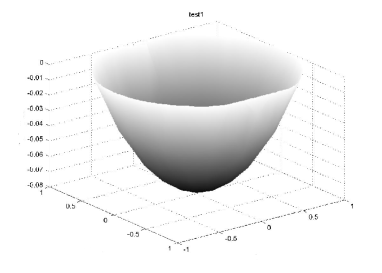
Figure 5.1. First test problem : Graph of $u_{h}^{c}.$

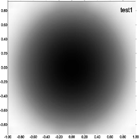
Figure 5.2. First test problem : Contour plot of $u_{h}^{c}.$

We conclude from the results in Table 1 that the value $g^{0}=0.3$ is optimal and quite accurate approximations of the exact solutions are obtained.

Remark 4.

We did not try to find the optimal value of $g^{0}$(it seems that is a difficult problem).

In the second test problem we take

$$f(x)={\displaystyle\left(\frac{4}{5}\right)^{2}\pi^{2}\left[\mbox{cos}^{2}\left(\frac{\pi}{2}\left(1-\left|x\right|^{2}\right)\right)+\frac{\pi}{2}\left(\left|x\right|^{2}\right)\mbox{sin}\left(\pi\left(1-\left|x\right|^{2}\right)\right)\right].}$$

The solution to the corresponding Monge-Ampère problem is the function $u\in C^{\infty}(\bar{\Omega})$ defined by

$$u\left(x\right)=-\frac{4}{5}\mbox{sin}\left(\frac{\pi}{2}\left(1-\left|x\right|^{2}\right)\right).$$

The method provides after 64 iterations the results summurized in Table 2.

The value $g^{0}=0.3$ is again optimal.

Table 2. second test problem : Convergence of the approximate solution.

$h$	$g_{h}^{0}$	$\left\|u-u_{h}^{c}\right\|_{0,\Omega}$
$\begin{array}[]{c}\nicefrac{{1}}{{32}}\\ \nicefrac{{1}}{{32}}\\ \nicefrac{{1}}{{32}}\end{array}$	$\begin{array}[]{c}0.1\\ 0.2\\ 0.3\end{array}$	$\begin{array}[]{c}0.6466\times 10^{-4}\\ 0.4510\times 10^{-4}\\ 0.2983\times 10^{-4}\end{array}$
$\begin{array}[]{c}\nicefrac{{1}}{{64}}\\ \nicefrac{{1}}{{64}}\\ \nicefrac{{1}}{{64}}\end{array}$	$\begin{array}[]{c}0.1\\ 0.2\\ 0.3\end{array}$	$\begin{array}[]{c}0.1749\times 10^{-4}\\ 0.8507\times 10^{-5}\\ 0.6221\times 10^{-5}\end{array}$
$\begin{array}[]{c}\nicefrac{{1}}{{128}}\\ \nicefrac{{1}}{{128}}\\ \nicefrac{{1}}{{128}}\end{array}$	$\begin{array}[]{c}0.1\\ 0.2\\ 0.3\end{array}$	$\begin{array}[]{c}0.3743\times 10^{-5}\\ 0.1180\times 10^{-5}\\ 0.5591\times 10^{-6}\end{array}$

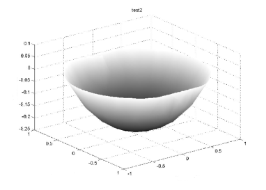
Figure 5.3. Second test problem : Graph of $u_{h}^{c}.$

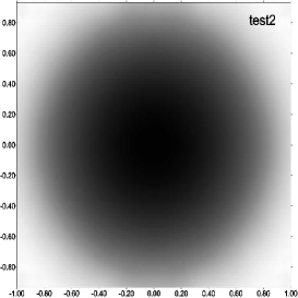
Figure 5.4. Second test problem : Contour plot of $u_{h}^{c}.$

The third test problem is defined as follows

(5.2) $$\left\{\begin{array}[]{cc}\mbox{det}[D^{2}u]=1&x\in\Omega,\\ u_{|\Gamma}=0,&u\>\textrm{convex}.\end{array}\right.$$

The function $u$ given by

$$u(x)=\frac{1}{2}\left(\left|x\right|^{2}-1\right)$$

is the solution of (5.2) and $u\in C^{\infty}(\bar{\Omega}).$

Table 3. Third test problem : Convergence of the approximate solution.

$h$	$g_{h}^{0}$	$\left\|u-u_{h}^{c}\right\|_{0,\Omega}$
$\begin{array}[]{c}\nicefrac{{1}}{{32}}\\ \nicefrac{{1}}{{32}}\\ \nicefrac{{1}}{{32}}\end{array}$	$\begin{array}[]{c}0.1\\ 0.2\\ 0.3\end{array}$	$\begin{array}[]{c}0.3830\times 10^{-3}\\ 0.2564\times 10^{-3}\\ 0.2971\times 10^{-3}\end{array}$
$\begin{array}[]{c}\nicefrac{{1}}{{64}}\\ \nicefrac{{1}}{{64}}\\ \nicefrac{{1}}{{64}}\end{array}$	$\begin{array}[]{c}0.1\\ 0.2\\ 0.3\end{array}$	$\begin{array}[]{c}0.7448\times 10^{-4}\\ 0.8529\times 10^{-6}\\ 0.9193\times 10^{-5}\end{array}$
$\begin{array}[]{c}\nicefrac{{1}}{{128}}\\ \nicefrac{{1}}{{128}}\\ \nicefrac{{1}}{{128}}\end{array}$	$\begin{array}[]{c}0.1\\ 0.2\\ 0.3\end{array}$	$\begin{array}[]{c}0.6215\times 10^{-5}\\ 0.5837\times 10^{-6}\\ 0.3806\times 10^{-5}\end{array}$

Figure 5.5. Third test problem : Graph of $u_{h}^{c}.$

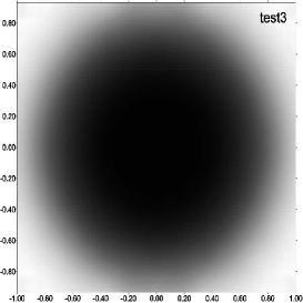
Figure 5.6. Third test problem : Contour plot of $u_{h}^{c}.$

We deduce from Table 3 that $g_{0}=0.2$ is an optimal value.

Unfortunaly I did not find any other initial value that gives more accurate results. Even for $g_{0}=0.4$ the results are not satisfied.

References

• [1] L. Armijo, Minimization of functions having Lipschits continuous partial derivatives, Pacific J. Math. 16 (1966) 1-3.
• [2] T. Aubin, Nonlinear analysis on manifolds, Monge-Ampère equations, Springer-Verlag, Berlin, 1982.
• [3] J. D. Benamou and Y. Brenier, The Monge-Kantorovich mass transfer and its computational fluid mechanics formulation, Int. J. Numer. Meth. Fluids, 2002.
• [4] J-D. Benamou, B. D. Frose, A. M. Oberman, Two numerical methods for the elliptic Monge-Ampere equation, ESSAIM: M2AN 44 (2010) 737-758.
• [5] O. Bokanowski, B. Grébert, Deformations of density functions in molecular quantum chemistry, J. Math. Phys. 37 (1996), no. 4, 1553-1573.
• [6] K. Böhmer, on finite element methods for fully nonlinear elliptic equations of second order, SIAM J. Numer. Anal., 46(3):1212-1249, 2008.
• [7] Y. Brenier, Some geometric PDEs related to hydrodynamics and electrodynamics, in Proceedings of the International Congress of Mathematicians, Beijing 2002, August 20-28, Vol. III, Higher Eduction Press, Beijing, 2002, pp. 761-771.
• [8] X. Cabré, Topics in regularity and qualitatives properties of solutions of non linear elliptic equations, Current developments in partial differential equations (Temucooo,1999). Discrete Contin. Dyn. Syst. 8 (2002). pp. 289-302.
• [9] L. Caffarelli, Non linear elliptic theory and the Monge-Ampère equation, in Proceedings of the International Congress of Mathematicians, Beijing 2002, August 20-28, Vol. I, Higher Eduction Press, Beijing, 2002, pp. 179-187.
• [10] L. Caffarelli and X. Cabré, Fully nonlinear Elliptic Equations, American Mathematical society, Providence, RI, 1995.
• [11] L. Caffarelli, S. A. Kochengin, V.I. Oliker, On the Numerical solution of the problem of reflector design with given far-field scattering data, Contemporary Mathematics, 226, (1999), 13-32. (Eds. L. A. Caffarelli and M. Milman)
• [12] L. Caffarelli, and Y. Y. Li, A liouville theorem for solutions of the Monge-Ampère equation with periodic data, Ann. Inst. H. Poincarè Anal. Non Linéaire, 21 (2004), pp. 97-120.
• [13] L. Caffarelli, L. Nirenberg, J. Spruck, The Dirichlet problem for nonlinear second-order elliptic equation I. Monge-Ampère equation, Comm. on Pure and Appl. Math., 17, (1984), 396-402.
• [14] L. Caffarelli, L Nirenberg, J. Spruck, The Dirichlet problem for the degenerate Monge-Ampère equation, Rev. Mat. Ibero., 2, (1985), 19-27.
• [15] S-Y. A. Chang and P. C. Yang, Nonlinear partial differential equations in conformal geometry, in Proceedings of the International Congress of Mathematicians, Beijing 2002, August 20-28, Vol. I, Higher Eduction Press, Beijing, 2002, pp. 189-207.
• [16] P. G. Ciarlet, The Finite Element Method for Elliptic Problems,North-Holland, Amsterdam (1978).
• [17] R. Courant, D. Hilbert, Methods of mathematical physics, Vol. II, New York Interscience Publishers, Wiley (1962).
• [18] M. J. P Cullen and R.J. Douglas, applications of the Monge-Ampère equation and Monge transport problem to metorology and oceanog-raphy, contemporary Mathematics, 226, (1999), 33-53.
• [19] E. J. Dean, R. Glowinski, Numerical solution of the two-dimensional elliptic Monge-Ampère equation with Dirichlet boundary conditions: an augmented Lagrangian approach, C. R. Acad. Sci. Paris, Ser. 1336 (2003) 779-784.
• [20] E. J. Dean, R. Glowinski, Numerical solution of the two-dimensional elliptic Monge-Ampère equation with Dirichlet boundary conditions: a least-squares approach, C. R. Acad. Sci. Paris, Ser. 1339 (2004) 887-892.
• [21] E. J. Dean, R. Glowinski, Numerical methods for fully nonlinear elliptic equations of the Monge-Ampère type, Comput. Methods Appl. Mech. Engrg., 195(13-16):1344-1386, 2006.
• [22] E. J. Dean, R. Glowinski, On the numerical solution of the elliptic Monge-Ampère equation in dimension two: a least-squares approach. In Partial differential equations, volume 16 of Comput. Methods Appl. sci., pages 43-63, Springer, Dordrecht, 2008.
• [23] X. Feng and M.Neilan, Vanishing moment method and moment solutions for second order fully nonlinear partial differential equations, J. Scient. Comp., DOI 10.1007/s10915-008-9221-9, 2008.
• [24] A. A. Goldstein, On steepest descent, SIAM J. Control 3 (1965) 147-151.
• [25] G. J. Haltiner, Numerical weather prediction, New York, Wiley (1971).
• [26] S.A. Kochengin, V.L. Oliker, Determination of reflector surfaces from near-filed scattering data, Inverse Problems 13 (1997), no. 2, 363-373.
• [27] F. X. Le Dimet and M. Ouberdous, Retrieval of balanced fields: an optimal control method, Tellus, 45 A (1993), pp. 449-461.
• [28] P.L. Lions. Une méthode nouvelle pour l’existense de solutions régulière de l’équation de Monge-Ampère réelle, C.R. Acad. Sc. Paris, T. 293, (30 Novombre 1981), Serie I, 589-592.
• [29] Michael Neilan A nonconforming Moreley finite element method for the fully nonlineair Monge-Ampere equation, Numer. Math. 115 (2010) 371-394.
• [30] E. Newman V.I. oliker, Differential-geometric methods in the design of reflector antennas, Sympos. Math., 35, (1992), 205-223.
• [31] Newman and L. Pamela Cook, A generalized Monge-Ampère equation arising in compressible Flow, Contemporary Mathematics, 226, (1999), 149-156.
• [32] A. M. Oberman, Wide stencil finite difference schemes for elliptic Monge-Ampère equation and functions of the eigenvalues of the Hessian, Discr. Cont. Dynam. Sys. B, 10(1):221-238, 2008.
• [33] V. Oliker, On the linearized Monge-Ampère equations related to the boundary value Minkowski problem and its generalizations. In : Gherardelli, F. (ed.) Monge-Ampère Equations and Related Topics, Proceedings of a seminar help in Firenze, 1980, pp. 79-112 Roma (1982).
• [34] V. I. Oliker, L. D. Prussner, On the numerical solution of th equation $z_{x}z_{y}-z_{xy}^{2}=f$ and its discretization, I, Numer. Math. 54 (1988) 271-293.
• [35] V. Oliker and P. Waltman, Radilly symmetric solutions of a Monge-Ampère eqaution arising in a reflector mapping problem, lecture notes in Mathematics 1285, EDS. A. Dold.
• [36] E. Polak, G. Ribière, Note sur la convergence de directions conjuguées, Rev. Francaise Infomat Recherche Operationnelle, 3e Année 16 (1969) 35-43.
• [37] B. T. Polyak, The conjugate gradient method in extreme problems, USSR Comput. Math. Math. Phys. 9 (1969) 94-112.
• [38] P. Wolfe, Convergence conditions for ascent methods, SIAM Rev. 11 (1969) 226-235.
• [39] V. Zheligovsky, O. Podvigina, U. Frish, The Monge-Ampère equation: Various forms and numerical solution, 229 issue 13 (2010).