Quantum-enhanced measurements without entanglement
Abstract
Quantum-enhanced measurements exploit quantum mechanical effects for increasing the sensitivity of measurements of certain physical parameters and have great potential for both fundamental science and concrete applications. Most of the research has so far focused on using highly entangled states, which are, however, difficult to produce and to stabilize for a large number of constituents. In the following we review alternative mechanisms, notably the use of more general quantum correlations such as quantum discord, identical particles, or non-trivial Hamiltonians; the estimation of thermodynamical parameters or parameters characterizing non-equilibrium states; and the use of quantum phase transitions. We describe both theoretically achievable enhancements and enhanced sensitivities, not primarily based on entanglement, that have already been demonstrated experimentally, and indicate some possible future research directions.
I Introduction
I.1 Aim and scope
Quantum-enhanced measurements aim at improving measurements of physical parameters by using quantum effects. The improvement sought is an enhanced sensitivity for a given amount of resources such as mean or maximum energy used, number of probes, number of measurements, and integration time. Ideas in this direction go back at least to the late 1960s when the effect of quantum noise on the estimation of classical parameters started to be studied in a systematic way using appropriate mathematical tools Helstrom (1969); Holevo (1982). In the early 1980s first detailed proposals appeared on how to enhance the sensitivity of gravitational wave detectors by using squeezed light Caves (1980, 1981). Nowadays, squeezed light is routinely produced in many labs, and used for instance to enhance sensitivity in gravitational wave observatories Aasi et al. (2013); Chua (2015).
Quantum-enhanced measurements have the potential of enabling many important applications, both scientific and technological. Besides gravitational wave detection, there are proposals or demonstrations for the improvement of time- or frequency-standards, navigation, remote sensing, measurement of very small magnetic fields (with applications to medical brain- and heart-imaging), measurement of the parameters of space-time, thermometry, and many more. The literature on the topic of quantum metrology is vast and for a general introduction we refer to the available reviews Wiseman and Milburn (2009); Paris (2009); Giovannetti et al. (2006); Pezzè and Smerzi (2014); Tóth and Apellaniz (2014); Pezzè et al. (2016); Degen et al. (2016).
From the theoretical side, the standard tool for evaluating a possible quantum enhancement has become the so-called quantum Cramér-Rao bound Helstrom (1969); Holevo (1982); Braunstein and Caves (1994); Braunstein et al. (1996). It provides a lower bound on the variance of any unbiased estimator function that maps observed data obtained from arbitrary quantum measurements to an estimate of the parameter . The bound is optimized over all possible measurements and data analysis schemes, in a sense made precise below. In the limit of an infinite number of measurements the bound can be saturated. It thus represents a valuable benchmark that can in principle be achieved once all technical noise problems have been solved, such that only the unavoidable noise inherent in the quantum state itself remains.
A standard classical method of noise reduction is to average measurement results from independent, identically prepared systems. In a quantum mechanical formulation with pure states, the situation corresponds to having the quantum systems in an initial product state, . Suppose that the parameter is encoded in the state through a unitary evolution with a Hamiltonian , i.e. . Based on the quantum Cramér-Rao bound one can show that with final measurements, the smallest achievable variance of the estimation of is
| (1) |
where and
are the largest and smallest eigenvalue of , respectively,
taken for simplicity here as identical for all subsystems
Giovannetti et al. (2006).
In fact, this scaling can be easily understood as a
consequence of the central limit theorem in the simplest case that one
measures the systems independently. But since (1)
is optimized over all measurements of the full system, it also implies
that entangling measurements of all systems after the parameter has
been encoded in the state cannot improve the scaling.
Unfortunately, there is no unique definition of the Standard Quantum Limit in the
literature. Whereas in the described scaling refers
to the number of distinguishable sub-systems, the term Standard Quantum Limit is used for
example in quantum optics typically for a scaling as
with the average number of photons , which in the same mode
are to be considered as indistinguishable (see Sec.III).
In this context, the scaling is
also called “shot-noise limit”, referring to the quantum noise that
arises from the fact that the electromagnetic energy is quantized in
units of photons. Furthermore, the prefactor in these scaling
behaviors is not fixed. We therefore may define quite generally Standard Quantum Limit
as the best scaling that can be achieved when employing only “classical” resources.
While this is not yet a mathematical definition either, it becomes precise once the classical resources are specified in the problem at hand. This may be achieved adopting a resource-theory framework, in which classical states of some specific sort are identified and formalised as “free” states (i.e. given at no cost), and any other state is seen as possessing a resource content which may allow us to outperform free states in practical applications, leading specifically to quantum-enhanced measurements beyond the Standard Quantum Limit scaling. For instance, separable states are the free (classical) states in the resource-theory of entanglement Horodecki et al. (2009), while states diagonal in a reference basis are the free (classical) states in the resource theory of quantum coherence Streltsov et al. (2017). In quantum optics, Glauber’s coherent states and their mixtures are regarded as the free (classical) states Mandel and Wolf (1965), and any other state can yield a nonclassical scaling. In the latter example, considering the mean photon number as an additional resource, one can fix the prefactor of the Standard Quantum Limit scaling, so that quantum enhancements are possible not only by improving the scaling law, but also by changing the prefactor.
However, basing our review exclusively on a resource-theory picture would be too restrictive, as cases of enhanced sensitivity are readily available for which no resource theory has been worked out yet (see Brandão and Gour (2015) and references therein for a recent overview of existing resource theories). Examples are the use of quantum phase transitions, for which one can compare the sensitivity at the phase transition with the sensitivities away from the phase transition, or instances of Hamiltonian engineering, for which one can evaluate the effect of added terms in the Hamiltonian. Rather than developing resource theories for all these examples, which would be beyond the scope of this review, we point out the enhancements achievable compared to the sensitivity without the use of the mechanism under consideration.
Based again on the quantum Cramér-Rao bound one can show that
initially entangled states can improve the scaling to
(see e.g. Giovannetti et al. (2006)), known as the
“Heisenberg-limit”. Similarly to the Standard Quantum Limit, there is no unique
definition of the Heisenberg-limit in the literature (see the remarks in sec.IV.1).
Nevertheless, achieving “the Heisenberg-limit” has been the goal of large experimental and
theoretical efforts over the last two decades. However, only few
experiments achieved the scaling of the Heisenberg-limit and only for very
small numbers of sub-systems, where the scaling advantage is
still far from allowing one to beat the best possible classical
measurements. This has several reasons: first of all, it is
already very difficult to achieve even the Standard Quantum Limit, as all
non-intrinsic noise sources have to be eliminated. Secondly,
resources such as photons are cheap, such that classically one can
operate with very large photon numbers, whereas entangled states
with large photon numbers are difficult to produce. Thirdly, and
most fundamentally, quantum-enhanced measurements schemes are plagued
by decoherence.
Indeed, it has been shown that a small amount of Markovian
decoherence brings the scaling for certain highly entangled
states back to the scaling of the Standard Quantum Limit
Huelga et al. (1997); Kołodyński and Demkowicz-Dobrzański (2010); Escher et al. (2011).
The reduction to the Standard Quantum Limit also affects the
estimation of noise in programmable and teleportation-covariant
channels Laurenza et al. (2017). Recent research has focussed on
finding optimal states in the presence of decoherence, and at
least for non-Markovian noise, a certain improvement can still be
obtained from entangled states
Chin et al. (2012); Matsuzaki et al. (2011). Also, niche
applications are possible, for which the light-intensity must be very
small, as in some biological applications. Nevertheless, it
appears worthwhile to think about alternative possible quantum
enhancement principles other than the use of highly entangled
states, and this is the focus of the
present survey.
Many results have been obtained over the last years for such
alternative schemes that are worth a comprehensive and exhaustive
review that compares their usefulness with respect to the main-stream
research focused on highly entangled states.
We structure the review by different ways of
breaking the conditions that are known to lead to Standard Quantum Limit scaling of the
sensitivity. Firstly, by going away from pure states, more general
forms of quantum correlations such as quantum discord become
possible. These become naturally important once we look at
estimation of loss parameters, quantum illumination problems, and
other applications that typically involve the loss of probes.
Secondly, in the derivation of the Standard Quantum Limit the quantum systems are
distinguished by an index , which supposes that they are
distinguishable. Cold atoms, on the other hand, have to be considered in general
as indistinguishable particles, and the same is true for photons,
which have been used for quantum-enhanced
measurements from the very beginning. Hence, statements about the
necessity of entanglement have to be re-examined for indistinguishable
particles. It turns out that the permutational symmetry of the
quantum states required due to
indistinguishability of the particles leads immediately to the level
of quantum-enhanced sensitivity that for distinguishable particles
would require to entangle them.
Thirdly, the structure of the Hamiltonian is rather
restrictive: a.) many hamitonians do not have a bound spectrum
characterized by largest and smallest eigenvalues and
as assumed in eq.(1). Indeed, one of the most common
systems used in quantum metrology, the harmonic oscillator that
represents e.g. a single mode of an electro-magnetic field, has an
unbound spectrum. And b.), the Hamiltonian does not
allow for any interactions. Taking into account these freedoms opens
the path to many new forms of enhanced sensitivity.
Fourthly, unitary evolutions with a
Hamiltonian that depends on the parameter are not the only way of
coding a parameter in a state. In statistical mechanics, for example,
there are parameters that describe the statistical ensemble, such as
temperature or chemical potential for systems in thermal equilibrium,
but which are not of Hamiltonian
origin. The same is true for non-equilibrium states. For many of these
situations, the corresponding QCRs have been obtained only recently,
and it often turned out that improvements beyond the Standard Quantum Limit should be
possible. Furthermore, it is known even in classical statistical
physics that phase transitions can lead to diverging susceptibilities
and hence greatly enhanced sensitivities. The same is true for quantum
phase transitions, and we therefore review as well the use of quantum
phase transitions for quantum-enhanced measurements.
While a growing number of researchers are investigating possibilities of breaking the Standard Quantum Limit without using entanglement (see e.g. Tilma et al. (2010)), these still appear to be a minority. The situation is comparable to other aspects and fields of quantum information treatment, where previously it was thought that entanglement is necessary. For example, for a long time entanglement has been considered as necessary for non-locality, until it was realized that certain aspects of non-locality can arise without entanglement Bennett et al. (1999). Recent reviews of quantum-enhanced measurements schemes using entanglement Paris (2009); Giovannetti et al. (2011); Pezzè and Smerzi (2014); Tóth and Apellaniz (2014); Pezzè et al. (2016); Degen et al. (2016) are available and we do not survey this vast literature here, but focus rather exclusively on quantum-enhanced measurements schemes that are not essentially based on the use of entanglement, hoping that our review will stimulate research in these directions. Before reviewing these schemes, we give a short introduction to parameter estimation theory and the precise definition of the quantum Cramér-Rao bound. A more elaborate pedagogical introduction to classical and quantum parameter estimation theory can be found in Fraïsse (2017).
I.2 Parameter estimation theory
Consider the following task in classical statistical analysis: Given a probability distribution of a random variable that continuously varies as function of a single real parameter , estimate as precisely as possible from samples drawn, i.e. a set of random values . We denote this -sample as for short, and denote the probability to find the drawn samples in the intervals as , with . For independently drawn, identically distributed samples, , but the formalism allows for arbitrary joint-probability distributions i.e. also correlations between different samplings of the distribution. For simplicity we take the support of to be the real numbers.
The task is accomplished by using an estimator function that takes as input the drawn random values and nothing else, and outputs an estimate of the parameter . Many different estimator functions are possible, some more useful than others. Through its random arguments the estimator will itself fluctuate from one sample to another. One would like to have an estimator that on average gives the true value of , , where is the mean value of a quantity over the distribution. This should hold at least in an infinitesimal interval about the true value of ; such an estimator is called “unbiased”. Secondly, one would like the estimator to fluctuate as little as possible. The latter request makes only sense together with the first one, as otherwise we could just choose a constant estimator, which of course would not reproduce the correct value of in most cases. Now consider the following chain of equalities, valid for an unbiased estimator:
| (2) | |||||
In the step before the last one we used that due to the normalization of the probability distribution valid for all values of . The scalar product in the last step is defined for any two real functions as . Using the Cauchy-Schwarz inequality for this scalar product, we immediately arrive at the (classical) Cramér-Rao (lower) bound for the variance of the estimator
| (3) |
where the (classical) Fisher information is defined as
| (4) | |||||
The bound can be saturated iff the two vectors in the scalar product are parallel, i.e. for , where is a possibly dependent proportionality factor. If one differentiates this condition once more and then integrates it over with , one finds that . Hence, an unbiased estimator exists iff there is a function independent of such that . In that case one can choose . One can show that for many (but not all) members of the family of exponential probability distributions, i.e. distributions that can be written in the form with some functions , this condition is satisfied, meaning that in such cases the Cramér-Rao bound can be saturated even for finite . For and identically, independently distributed samples, the so-called maximum-likelihood estimator saturates the bound. One easily shows from eq.(4) that the Fisher information is additive, such that for independently drawn, identically distributed samples with .
I.3 Quantum parameter estimation theory
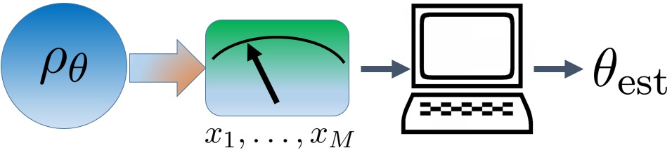
In quantum mechanics the state of a system is given by a density matrix , i.e. a positive hermitian operator with trace equal one that can depend on the parameter , which we assume to be a classical parameter. Random data are created when measuring some observable of the system whose statistics will depend on through the quantum state . Again we would like to estimate as precisely as possible based on the measurement data (see FIG.1).
The most general measurements are so-called POVM measurements (POVM=positive-operator-valued measure). These are measurements that generalize and include projective von Neumann measurements and are relevant in particular when the system is measured through an ancilla system to which it is coupled Peres (1993). They consist of a set of positive operators , where labels possible measurement outcomes that we take again as for simplicity. They obey a completeness relation, , where is the identity operator on the Hilbert-space of the system. The probability-density to find outcome is given by , and it is through this equation that the contact with the classical parameter estimation theory can be made: Plugging in in eq. (4) with , we are led to the Fisher information
| (5) | |||||
where in the last step we have introduced the so-called symmetric logarithmic derivative , defined indirectly through
| (6) |
in analogy to the classical logarithmic derivative . Compared to the classical case, one has in the quantum mechanical setting the additional freedom to choose a suitable measurement in order to obtain a distribution that contains as much information as possible on the parameter . Based on eq. (5), one can find a similar chain of inequalities as in the classical case based on the Cauchy-Schwarz inequality that leads to the bound
| (7) |
where is known as the “quantum Fisher information”.
Similarly as for the classical Fisher information, the quantum Fisher information of uncorrelated states is additive, Fujiwara and Hashizumé (2002):
| (8) |
such that for independent identical POVM measurements of the same system, prepared always in the same state, the total quantum Fisher information satisfies with . Inequalities (7) and (3) then lead to the so-called quantum Cramér-Rao bound,
| (9) |
Additivity of the quantum Fisher information also immediately implies the scaling
in eq.(1), as
the quantum Fisher information of the uncorrelated subsystems is just
times the quantum Fisher information of a single subsystem.
Inequality (7) can be saturated with a POVM that
consists of projectors onto eigenstates of
Helstrom (1969); Holevo (1982); Braunstein and Caves (1994).
As the quantum Cramér-Rao bound is already optimized, no
measurement of the whole system, even if entangling the individual systems, can
improve the sensitivity when the parameter was already imprinted on a
product state.
The quantum Cramér-Rao bound has become the most widely used quantity for establishing the ultimate sensitivity of measurement schemes. It derives its power from the facts that firstly it is already optimized over all possible data analysis schemes (unbiased estimator functions) and all possible (POVM-) measurements, and that secondly it can be saturated at least in the limit of infinitely many measurements and using the optimal POVM consisting of projectors onto the eigenstates of .
In Braunstein and Caves (1994) it was shown that is a geometric measure on how much and differ, where is an infinitesimal increment of . The geometric measure is given by the Bures-distance,
| (10) |
where the fidelity is defined as
| (11) |
and denotes the trace norm Miszczak et al. (2009). With this Braunstein and Caves (1994) showed that
| (12) |
unless the rank of changes with and thus produces removable singularities Banchi et al. (2015); Šafránek (2017), a situation which we do not consider in this review. The quantum Cramér-Rao bound thus offers the physically intuitive picture that the parameter can be measured the more precisely the more strongly the state depends on it. For pure states , the quantum Fisher information reduces to the overlap of the derivative of the state with itself and the original state Braunstein et al. (1996); Paris (2009),
| (13) |
If the parameter is imprinted on a pure state via a unitary transformation with hermitian generator as , eq.(13) gives . With a maximally entangled state of the subsystems and a suitable measurement, one can reach a scaling of the quantum Fisher information proportional to Giovannetti et al. (2006), the mentioned Heisenberg-limit. This can be seen most easily for a pure state of the form , where and are two eigenstates of to two different eigenvalues .
For mixed states, the Bures-distance is in general difficult to calculate, but is a convex function of , i.e. for two density matrices and and we have Fujiwara (2001a)
| (14) |
This can be used to obtain an upper bound for the quantum Fisher information. Convexity also
implies that the precision of measurements cannot be
increased by classically mixing states with mixing probabilities
independent of the parameter Braun (2010).
In principle, the optimal measurement that saturates the quantum Cramér-Rao bound can be
constructed by diagonalizing . The projectors onto its
eigenstates form a POVM that yields the optimal measurement. However,
such a construction requires that the precise value of the parameter
is already known. If that was the case, one could skip the
measurement altogether and choose the estimator as , with vanishing
uncertainty, i.e. apparently violating the quantum Cramér-Rao bound in most cases
Chapeau-Blondeau (2015) (note, however, that for a
state that depends on , the condition
for an unbiased estimator
cannot be fulfilled in a whole -interval about ,
such that there is no formal contradiction). If
is not
known, the more common
approach is therefore to use the quantum Cramér-Rao bound as a benchmark as function
of , and then
check whether physically motivated measurements can achieve it.
More general schemes have been proposed to mitigate the
problem of prior knowledge of the parameter. This includes the van
Trees inequality
van Trees (2001); Gill and Levit (1995), Bayesian approaches
Rivas and Luis (2012); Macieszczak et al. (2014), adaptive measurements
Serafini (2012); Okamoto et al. (2012); Wheatley et al. (2010); Berry and Wiseman (2006, 2013, 2002, 2000); Armen et al. (2002); Wiseman (1995); Fujiwara (2006); Higgins et al. (2009),
and
approaches specialized to
particular parameter estimation problems such as phase estimation
Hall et al. (2012).
Another point to be kept in mind is that the quantum Cramér-Rao bound can be reached
asymptotically for a large number of
measurements, but not necessarily for a finite number of
measurements. The latter case is clearly relevant for experiments and
subject of active current research (see
e.g. Liu and Yuan (2016)
).
These limitations not withstanding, we base this review almost
exclusively on the quantum Cramér-Rao bound (with the exception of Sec.II.7 on
quantum channel discrimination and parts of Sec.IV.2.1, where a
signal-to-noise ratio is used), given that the overwhelming majority of
results have been obtained for it and allow an in-depth
comparison of different strategies. A certain number of results
have been obtained as well for the quantum Fisher information optimized over all input
states Fujiwara (2001b); Fujiwara and Imai (2003), a quantity sometimes
called channel quantum Fisher information. We do not review this
literature here, as in this type of work sensitivity is typically not
separately optimized over entangled or
non-entangled initial states.
The Fisher information can be generalized to multi-parameter estimation Helstrom (1969); Paris (2009), . The Bures distance between two infinitesimal close states then reads
| (15) |
An expansion of leads to the quantum Fisher information matrix Sommers and Zyczkowski (2003); Paris (2009),
| (16) |
where , and is the symmetric logarithmic derivative with respect to parameter . The quantum Cramér-Rao bound generalizes to a lower bound on the co-variance matrix of the parameters Helstrom (1969, 1976); Paris (2009),
| (17) |
where , and means that is a positive-semidefinite matrix. Contrary to the single parameter quantum Cramér-Rao bound, the bound (17) can in general not be saturated, even in the limit of infinitely many measurements. The Bures metric has also been called fidelity susceptibility in the framework of quantum phase transitions Gu (2010).
II Quantum correlations beyond entanglement
II.1 Parallel versus sequential strategies in unitary quantum metrology
One of the most typical applications of quantum metrology is the task of unitary parameter estimation, exemplified in particular by phase estimation Giovannetti et al. (2006, 2011). Let be a unitary transformation, with the unknown parameter to be estimated, and a selfadjoint Hamiltonian operator which represents the generator of the transformation. The typical estimation procedure then consists of the following steps: a) preparing an input probe in a state ; b) propagating the state with the unitary transformation ; c) measuring the output state ; d) performing classical data analysis to infer an estimator for the parameter .
Let us now assume one has the availability of utilizations of the transformation . Then, the use of uncorrelated probes in a global initial state , each of which is undergoing the transformation in parallel, yields an estimator whose minimum variance scales as (Standard Quantum Limit). On the other hand, by using an initial entangled state of the probes, and propagating each with the unitary in parallel, one can in principle achieve the Heisenberg-limit, meaning that an optimal estimator can be constructed whose asymptotic variance, in the limit , scales as . However, it is not difficult to realize that the very same precision can be reached without the use of entanglement, by simply preparing a single input probe in a superposition state with respect to the eigenbasis of the generator , and letting the probe undergo sequential iterations of the transformation .
For instance, thinking of each probe as a qubit for simplicity, and fixing the generator to be the Pauli matrix , one can either consider a parallel scheme with input probes in the Greenberger-Horne-Zeilinger (GHZ, or cat-like) maximally entangled state , or a sequential scheme with a single probe in the superposition . In the first case, the state after imprinting the parameter reads , while in the second case . Hence, in both schemes one achieves an -fold increase of the phase between two orthogonal states, and both schemes reach therefore the Heisenberg-limit scaling in the estimation of the phase shift , meaning that the quantum Cramér-Rao bound can be asymptotically saturated in both cases by means of an optimal measurement, associated to a quantum Fisher information scaling quadratically with . The equivalence between entanglement in parallel schemes and coherence (namely, superposition in the eigenbasis of the generator) Baumgratz et al. (2014); Streltsov et al. (2017); Marvian and Spekkens (2016) in sequential schemes further extends to certain schemes of quantum metrology in the presence of noise, namely when the unitary encoding the parameter to be estimated and the noisy channel commute with each other (e.g. in the case of phase estimation affected by dephasing) Boixo and Heunen (2012); Demkowicz-Dobrzański and Maccone (2014), although in more general instances entanglement is shown to provide an advantage Huelga et al. (1997); Escher et al. (2011); Demkowicz-Dobrzański and Maccone (2014). In general, sequential schemes such that individual probes are initially correlated with an ancilla (on which the parameter is not imprinted) and assisted by feedback control (see Sec. IV.6.4) can match or outperform any parallel scheme for estimation of single or multiple parameters encoded in unitary transformations even in the presence of noise Demkowicz-Dobrzański and Maccone (2014); Sekatski et al. (2017); Huang et al. (2016); Yuan and Fung (2015); Yuan (2016); Nichols et al. (2016); Yousefjani et al. (2017). While probe and ancilla typically need to be entangled for such sequential schemes to achieve maximum quantum Fisher information, this observation removes the need for large-scale multiparticle entangled probes in the first place.
Similarly, in continuous variable optical interferometry Caves (1981), equivalent performances can be reached (for unitary phase estimation) by using either a two-mode entangled probe, such as a N00N state, or a single-mode non-classical state, such as a squeezed state. These are elementary examples of quantum-enhanced measurements achievable without entanglement, yet exploiting genuinely quantum effects such as nonclassicality and superposition. Such features can be understood by observing that both optical nonclassicality in infinite-dimensional systems and coherence (superposition) in finite-dimensional systems can be converted to entanglement within a well-defined resource-theoretic framework Asbóth et al. (2005); Vogel and Sperling (2014); Streltsov et al. (2015); Killoran et al. (2016), and can be thought-of as equivalent resources to entanglement for certain practical purposes, as is evidently the case for unitary metrology. 111An additional scenario in which the quantum limit can be reached without entanglement is when a multipartite state is used to measure multiple parameters, where each parameter is encoded locally onto only one subsystem — it has recently been shown that entanglement between the subsystems is not advantageous, and can even be detrimental, in this setting Knott et al. (2016); Proctor et al. (2018).
II.2 General results on the usefulness of entanglement
More generally, for unitary metrology with multipartite probes in a parallel setting, a quite general formalism has been developed to identify the metrologically useful correlations in the probes in order to achieve quantum-enhanced measurements Pezzè and Smerzi (2009) (see Pezzè and Smerzi (2014); Tóth and Apellaniz (2014) for recent reviews). Specifically, let us consider an input state of qubits and a linear interferometer with Hamiltonian generator given by , i.e. a component of the collective (pseudo-)angular momentum of the probes in the direction , with denoting the th Pauli matrix for qubit . If is -producible, i.e., it is a convex mixture of pure states which are tensor products of at most -qubit states, then the quantum Fisher information is bounded above as follows Tóth (2012); Hyllus et al. (2012),
| (18) |
where is the integer part of . This means that genuine multipartite entangled probes () are required to reach the maximum sensitivity, given by the Heisenberg-limit , even though partially entangled states can still result in quantum-enhanced measurements beyond the Standard Quantum Limit.
A similar conclusion has been reached in Augusiak et al. (2016) considering the geometric measure of entanglement, which quantifies how far is from the set of fully separable (-producible) states according to the fidelity. Namely, for unitary metrology with parallel probes initialized in the mixed state , in the limit a nonvanishing value of the geometric measure of entanglement of is necessary for the exact achievement of the Heisenberg-limit. However, a sensitivity arbitrarily close to the Heisenberg-limit, for any , can still be attained even if the geometric measure of entanglement of vanishes asymptotically for . In deriving these results, the authors proved an important continuity relation for the quantum Fisher information in unitary dynamics Augusiak et al. (2016).
II.3 Role of quantum discord in parameter estimation with mixed probes
Here we will focus our attention on possible advantages stemming from the use of quantum correlations more general than entanglement in the (generally mixed) state of the input probes for a metrological task. Such correlations are usually referred to under the collective name of quantum discord Ollivier and Zurek (2001); Henderson and Vedral (2001), see also Modi et al. (2012); Adesso et al. (2016) for recent reviews. The name quantum discord originates from a mismatch between two possible quantum generalizations of the classical mutual information, a measure of correlations between two (or more) variables described by a joint probability distribution Ollivier and Zurek (2001). A direct generalization leads to the so-called quantum mutual information , that quantifies total correlations in the state of a bipartite system , with being the von Neumann entropy. An alternative generalization leads instead to , a measure of one-sided classical correlations that quantifies how much the marginal entropy of, say, subsystem is decreased (i.e., how much additional information is acquired) by performing a minimally disturbing measurement on subsystem described by a POVM , with being the conditional state of the system after such measurement Henderson and Vedral (2001). The difference between the former and the latter quantity is precisely the quantum discord,
| (19) |
that quantifies therefore just the quantum portion of the total correlations in the state from the perspective of subsystem . It is clear from the definition above that the state of a bipartite system has nonzero discord (from the point of view of ) if and only if it is altered by all possible local measurements performed on subsystem : disturbance by measurement is a genuine quantum feature which is captured by the concept of discord, see Modi et al. (2012); Adesso et al. (2016) for more details. Every entangled state is also discordant, but the converse is not true; in fact, almost all separable states still exhibit nonzero discord Ferraro et al. (2010). The only bipartite states with zero discord, from the point of view of subsystem , are so-called classical-quantum states, which take the form
| (20) |
where the states form an orthonormal basis for subsystem , and denote a set of arbitrary states for subsystem , while stands for a probability distribution. These states are left invariant by measuring in the basis , which entails that .
In a multipartite setting, one can define fully classical states as the states with zero discord with respect to all possible subsystems, or alternatively as the states which are left invariant by a set of local measurements performed on all subsystems. Such states take the form for an -particle system ; i.e., they are diagonal in a local product basis. One can think of these states as the only ones which are completely classically correlated, that is, completely described by a classical multivariate probability distribution , embedded into a density matrix formalism. An alternative way to quantify discord in a (generally multipartite) state is then by taking the distance between and the set of classically correlated states, according to a suitable (quasi)distance function. For instance, the relative entropy of discord Modi et al. (2010) is defined as
| (21) |
where the minimization is over all classically correlated states , and denotes the quantum relative entropy. For a dedicated review on different measures of discord-type quantum correlations we refer the reader to Adesso et al. (2016).
Let us now discuss the role of quantum discord in metrological contexts. Modi et al. (2011) investigated the estimation of a unitary phase applied to each of qubit probes, initially prepared in mixed states with either (a) no correlations; (b) only classical correlations; or (c) quantum correlations (discord and/or entanglement). All the considered families of -qubit probe states were chosen with the same spectrum, i.e. in particular the same degree of mixedness (which is a meaningful assumption if one is performing a metrology experiment in an environment with a fixed common temperature), and were selected due to their relevance in recent nuclear magnetic resonance (NMR) experiments Jones et al. (2009). In particular, given an initial thermal state for each single qubit (with purity parameter ), the product states were considered for case (a), and the GHZ-diagonal states were considered for case (c), with denoting the single-qubit Hadamard gate (acting on each qubit in the first case, and only on the first qubit in the second case), and C-Not1j a series of Control-Not operations acting on pairs of qubits and . These two classes of states give rise to quantum Fisher information and , respectively. By comparing the two cases, the authors of Modi et al. (2011) concluded that a quantum enhancement, scaling as , is possible using pairs of mixed probe states with arbitrary (even infinitesimally small) degree of purity. This advantage persists even when the states in strategy (c) are fully separable, which occurs for (with and determined numerically for each value of ), in which case both strategies are unable to beat the Standard Quantum Limit, yet the quadratic enhancement of (c) over (a) is maintained, being independent of . The authors then argue that multipartite quantum discord — which increases with according to the relative entropy measure of eq. (21) and vanishes only at — may be responsible for this enhancement. Let us remark that, even though the quantum Fisher information is convex (which means that for every separable but discordant mixed state there exists a pure product state with a higher or equal quantum Fisher information), the analysis in Modi et al. (2011) was performed at fixed spectrum (and thus degree of purity) of the input probes, a constraint which allowed the authors to still identify an advantage in using correlations weaker than entanglement, as opposed to no correlations. However, it is presently unclear whether these conclusions are special to the selected classes of states, or can be further extended to more general settings, including noisy metrology.
In a more recent work, Cable et al. (2016) analyzed a model of unitary quantum metrology inspired by the computational algorithm known as deterministic quantum computation with one quantum bit (DQC1) or “power of one-qubit” Knill and Laflamme (1998). Using only one pure qubit supplemented by a register of maximally mixed qubits, all individually subject to a local unitary phase shift , their model was shown to achieve the Standard Quantum Limit for the estimation of , which can be conventionally obtained using the same number of qubits in pure uncorrelated states. They found that the Standard Quantum Limit can be exceeded by using one additional qubit, which only contributes a small degree of extra purity, which, however, for any finite amount of extra purity leads to an entangled state at the stage of parameter encoding. In this model, incidentally, the output state after the unitary encoding was found to be always separable but discordant, with its discord vanishing only in the limit of vanishing variance of the estimator for the parameter . It is not quite clear if and how the discord in the final state can be interpreted in terms of a resource for metrology, but the achievement of the Standard Quantum Limit with all but one probes in a fully mixed state was identified as a quantum enhancement without the use of entanglement. This suggests that further investigation on the role of quantum discord (as well as state purity) in metrological algorithms with vanishing entanglement may be in order. A protocol for multiparameter estimation using DQC1 was studied in Boixo and Somma (2008), although the resource role of correlations was not discussed there. In MacCormick et al. (2016) a detailed investigation of a DQC1-based protocol was made based on coherently controlled Rydberg interactions between a single atom and an atomic ensemble containing atoms. The protocol allows one to estimate a phase shift assumed identical for all atoms in the atomic ensemble with a sensitivity that interpolates smoothly between Standard Quantum Limit and Heisenberg-limit when the purity of the atomic ensemble increases from a fully mixed state to pure states. It leads to a cumulative phase shift proportional to , and the scheme can in fact also be seen as an implementation of “coherent averaging”, with the control qubit playing the role of the “quantum bus” (see Sec. IV.6.3).
II.4 Black-box metrology and the interferometric power
As explicitly discussed in Sec. II.1, for unitary parameter estimation, if one has full prior information on the generator of the unitary transformation imprinting the parameter , then no correlations are required whatsoever, and probe states with coherence in the eigenbasis of suffice to achieve quantum-enhanced measurements in a sequential scheme. Recently, Girolami et al. (2013, 2014); Adesso (2014) investigated quantum metrology in a so-called black-box paradigm, according to which the generator is assumed not fully known a priori. In such a case, suppose one selects a fixed (but arbitrary) input single-particle probe , then it is impossible to guarantee a precision in the estimation of for all possible nontrivial choices of . This is because, in the worst case scenario, the black-box unitary transformation may be generated by a which commutes with the input state , resulting in no information imprinted on the probe, hence in a vanishing quantum Fisher information. It is clear then that, to be able to estimate parameters independently of the choice of the generator, one needs an ancillary system correlated with the probe. But what type of correlations are needed? It is in this context that discord-type correlations, rather than entanglement or classical correlations, are found to play a key resource role.
Consider a standard two-arm interferometric configuration, and let us retrace the steps of parameter estimation in the black-box scenario Girolami et al. (2014): a) an input state of two particles, the probe and the ancilla , is prepared; b) particle is transmitted with no interaction, while particle enters a black-box where it undergoes a unitary transformation generated by a Hamiltonian , whose spectrum is known but whose eigenbasis is unknown at this stage; c) the agent controlling the black-box announces the full specifics of the generator , so that parties and can jointly perform the best possible measurement on the two-particle output state ; d) the whole process is iterated times, and an optimal unbiased estimator is eventually constructed for the parameter . In the limit , for any specific black-box setting , the corresponding quantum Fisher information determines the maximal precision enabled by the input state in estimating the parameter generated by , as prescribed by the quantum Cramér-Rao bound.
One can then introduce a figure of merit quantifying the worst case precision guaranteed by the state for the estimation of in this black-box protocol. This is done naturally by minimizing the quantum Fisher information over all generators within the given spectral class (the spectrum is assumed nondegenerate, with a canonical choice being that of equispaced eigenvalues) Girolami et al. (2013, 2014). This defines (up to a normalization constant) the interferometeric power of the bipartite state with respect to the probing system ,
| (22) |
Remarkably, as proven in Girolami et al. (2014), the interferometric power turns out to be a measure of discord-type correlations in the input state . In particular, it vanishes if and only if takes the form of a classical-quantum state, eq. (20). This entails that states with zero discord cannot guarantee a precision in parameter estimation in the worst case scenario, while any other bipartite state (entangled or separable) with nonzero discord is suitable for estimating parameters encoded by a unitary transformation (acting on one subsystem) no matter the generator, with minimum guaranteed precision quantified by the interferometric power of the state. This conclusion holds both for parameter estimation in finite-dimensional systems Girolami et al. (2014), and for continuous-variable optical interferometry Adesso (2014). Recently, it has been shown more formally that entanglement accounts only for a portion of the quantum correlations relevant for bipartite quantum interferometry. In particular, the interferometric power, which is by definition a lower bound to the quantum Fisher information (for any fixed generator ), is itself bounded from below in bipartite systems of any dimension by a measure of entanglement aptly named the interferometric entanglement, which simply reduces to the squared concurrence for two-qubit states Bromley et al. (2017). The interferometric power can be evaluated in closed form, solving analytically the minimization in eq. (22), for all finite-dimensional states such that subsystem is a qubit Girolami et al. (2014), and for all two-mode Gaussian states when the minimization is restricted to Gaussian unitaries Adesso (2014). An experimental demonstration of black-box quantum-enhanced measurements relying on discordant states as opposed to classically correlated states has been reported using a two-qubit NMR ensemble realized in chloroform Girolami et al. (2014).
We finally notice that, while (quantum) correlations with an ancilla are required to achieve a nonzero worst case precision when minimizing the quantum Fisher information over the choice of the generator within a fixed spectral class, as in the scenario considered here, single-probe (non-maximally mixed) states may however suffice to be useful resources in the arguably more practical case in which the average precision, rather than the minimal, is considered instead as a figure of merit. This scenario is further discussed in Sec. II.8.
II.5 Quantum estimation of bosonic loss
Any quantum optical communication, from fibre-based to free-space implementations, is inevitably affected by energy dissipation. The fundamental model to describe this scenario is the lossy channel. This attenuates an incoming bosonic mode by transmitting a fraction of the input photons, while sending the other fraction into the environment. The maximum number of bits per channel use at which we can transmit quantum information, distribute entanglement or generate secret keys through such a lossy channel are all equal to Pirandola et al. (2017), a fundamental rate-loss tradeoff that only quantum repeaters may surpass Pirandola (2016). For these and other implications to quantum communication, it is of paramount importance to estimate the transmissivity of a lossy channel in the best possible way.
Quantum estimation of bosonic loss was first studied in Monras and Paris (2007) by using single-mode pure Gaussian states (see also Pinel et al. (2013)). In this setting, the performance of the coherent state probes at fixed input energy provides the shot-noise limit or classical benchmark, which has to be beaten by truly quantum probes. Let us denote by the mean number of photons, then the shot-noise limit is equal to Monras and Paris (2007); Pinel et al. (2013). The use of squeezing can beat this limit, following the original intuition for phase estimation of Caves (1981). In fact, Monras and Paris (2007) showed that, in the regime of small loss and small energy , a squeezed vacuum state can beat the Standard Quantum Limit. The use of squeezing for estimating the interaction parameter in bilinear bosonic Hamiltonians (including beam-splitter interactions) was also discussed in Gaiba and Paris (2009), showing that unentangled single-mode squeezed probes offer equivalent performance to entangled two-mode squeezed probes for practical purposes.
The optimal scaling can be achieved by using Fock states at the input Adesso et al. (2009). Note that, because Fock states can only be used when the input energy corresponds to integer photon numbers, in all the other cases one needs to engineer superpositions, e.g., between the vacuum and the one-photon Fock state if we want to explore the low-energy regime . Non-Gaussian qutrit and quartet states can be designed to beat the best Gaussian probes Adesso et al. (2009). It is still an open question to determine the optimal probes for estimating loss at any energy regime. It is certainly known that the bound holds for any , as it can be proven by dilating the lossy channel into a beam-splitter unitary and then performing parameter estimation Monras and Paris (2007). Note that this bound is computed by considering uncorrelated probes in parallel. It is therefore an open question to find the best performance that is achievable by the most general (adaptive) strategies.
Interestingly, the problem of estimating the loss parameters of a pair of lossy bosonic channels has been proven formally equivalent to the problem of estimating the separation of two incoherent optical point-like sources Lupo and Pirandola (2016). In this context Tsang et al. (2016) showed that a pair of weak thermal sources can be resolved independently from their separation if one adopts quantum measurements based on photon counting, instead of standard intensity measurements. Thus, quantum detection strategies enables one to beat the so-called “Rayleigh’s curse” which affects classical imaging Tsang et al. (2016). This curse is reinstated in the classical limit of very bright thermal sources Lupo and Pirandola (2016); Nair, R. and Tsang, T. (2016). On the other hand, Lupo and Pirandola (2016) showed that quantum-correlated sources can be super-resolved at the sub-Rayleigh scale. In fact, it is possible to engineer quantum-correlated point-like sources that are not entangled (but discordant) which displays super-resolution, so that the closer the sources are the better their distance can be estimated.
The estimation of loss becomes complicated in the presence of decoherence, such as thermal noise in the environment and non-unit efficiency of the detectors. From this point of view, Spedalieri et al. (2016) considered a very general model of Gaussian decoherence which also includes the potential presence of non-Markovian memory effects. In such a scenario, Spedalieri et al. (2016) showed the utility of asymmetrically correlated thermal states (i.e., with largely different photon numbers in the two modes), fully based on discord and void of entanglement. These states can be used to estimate bosonic loss with a sensitivity that approaches the shot noise limit and may also surpass it in the presence of correlated noise and memory effects in the environment. This kind of thermal quantum metrology has potential applications for practical optical instruments (e.g., photometers) or at different wavelengths (e.g., far infrared, microwave or X-ray) for which the generation of quantum features, such as coherence, number states, squeezing or entanglement, may be challenging.
II.6 Gaussian quantum metrology
Clearly we may also consider the estimation of other parameters beyond loss. In general, Gaussian quantum metrology aims at estimating any parameter or multiple parameters encoded in a bosonic Gaussian channel. As shown in Pirandola and Lupo (2017), the most general adaptive estimation of noise parameters (such as thermal or additive noise) cannot beat the Standard Quantum Limit. This is because Gaussian channels are teleportation-covariant, i.e., they suitably commute with the random operations induced by quantum teleportation, a property which is shared by large class of quantum channels at any dimension Pirandola et al. (2017). The joint estimation of specific combinations of parameters, such as loss and thermal noise, or the two real components of a displacement, has been widely studied in the literature Monras and Illuminati (2011); Bellomo et al. (2009, 2010b, 2010a); Genoni et al. (2013); Gao and Lee (2014); Duivenvoorden et al. (2017); Gagatsos et al. (2016), but the ultimate performance achievable by adaptive (i.e., feedback-assisted) schemes is still unknown.
If we employ Gaussian states at the input of a Gaussian channel, then we have Gaussian states at the output and we may exploit closed formulas for the quantum Fisher information. These formulas can be derived by direct evaluation of the symmetric logarithmic derivative Monras (2013); Jiang (2014); Šafránek et al. (2015); Nichols et al. (2017) or by considering the infinitesimal expression of the quantum fidelity Banchi et al. (2015); Pinel et al. (2013, 2012). The latter approach may exploit general and handy formulas. In fact, for two arbitrary multi-mode Gaussian states, and , with mean values and , and covariance matrices and , we may write the Uhlmann-Jozsa fidelity Banchi et al. (2015)
| (23) | |||||
| (24) |
where we set with being the symplectic form Banchi et al. (2015). Specific expressions for the fidelity were previously given for single-mode Gaussian states Scutaru (1998), two-mode Gaussian states Marian and Marian (2012), multi-mode Gaussian states assuming that one of the states is pure Spedalieri et al. (2013), and multi-mode squeezed thermal Gaussian states with vanishing first moments Paraoanu and Scutaru (2000).
From eq. (23) we may derive the Bures metric . In fact, consider two infinitesimally-close Gaussian states , with statistical moments and , and , with statistical moments and . Expanding at the second order in and , one finds Banchi et al. (2015)
| (25) |
where , , and the inverse of the superoperator refers to the pseudo-inverse. A similar expression was also computed by Monras (2013) using the symmetric logarithmic derivative, with further refinements in Šafránek et al. (2015). From the Bures metric in eq. (25) we may derive the quantum Fisher information (see eq. (12)) for the estimation of any parameter encoded in a multi-mode (pure or mixed) Gaussian state directly in terms of the statistical moments. Eq. (25) is written in a compact basis-independent and parametrization-independent form, valid for any multi-mode Gaussian state. For an explicit parametrization via multiple parameters , one can expand the differential and write , and similarly for . In this way, as in Eq. (16), with
| (26) |
Eqs. (25) and (26) have been derived following eq. (12), namely explicitly computing the fidelity function for two most general multi-mode Gaussian states, and then taking the limit of two infinitesimally close states. A similar approach was used for fermionic Gaussian states in Banchi et al. (2014).
An alternative derivation of the bosonic quantum Fisher information for multi-mode Gaussian states, based on the use of the symmetric logarithmic derivative, has been recently obtained in Nichols et al. (2017). Furthermore, Nichols et al. (2017) derived a necessary and sufficient compatibility condition such that the quantum Cramér-Rao bound eq. (17) is asymptotically achievable in multiparameter Gaussian quantum metrology, meaning that a single optimal measurement exists which is able to extract the maximal information on all the parameters simultaneously. For any pair of parameters , in terms of the symmetric logarithmic derivatives and , the corresponding quantum Fisher information matrix element is defined as , while the measurement compatibility condition amounts to Ragy et al. (2016). In terms of the first and second statistical moments and of a -mode Gaussian state , we have then Nichols et al. (2017):
| (27) | |||||
with , where , are the symplectic eigenvalues of the covariance matrix , is the symplectic transformation that brings into its diagonal form, , and the set of matrices have all zero entries except for the block in position which is given by . Note that eq. (27) can also be obtained from (25) by explicitly writing all the operators in the basis in which is diagonal, observing that . On the other hand, Eq. (LABEL:eq:gcompatibility) cannot be obtained from the limit of the fidelity formula.
In the context of this review, Pinel et al. (2012) studied in particular the quantum Cramér-Rao bound for estimating a parameter which is encoded in a pure multi-mode Gaussian state. It was realized that, in the limit of large photon number, no entanglement nor correlations between different modes are necessary for obtaining the optimal sensitivity. Rather, a detection mode can be used based on the derivative of the mean photon field with respect to the parameter , into which all the resources in terms of photons and squeezing should be put. The mean photon field is defined as , with all parameter dependence in the pure Gaussian quantum state , , where are orthonormal mode functions found from solving Maxwell’s equation with appropriate boundary conditions, is the annihilation operators of mode , and the sum is over all modes. The mean field can be normalized, , where the norm contains spatial integration over a surface perpendicular to the light beam propagation and temporal integration over the detection time. The detection mode is then defined as , where ′ means derivative with respect to . The detection mode can be complemented by other, orthonormal modes to obtain a full basis, but these other modes need not be excited for achieving maximum quantum Fisher information. The quantum Fisher information reads then
| (29) |
where is the mean photon number, and the matrix element of the inverse covariance matrix of the Gaussian state corresponding to the detection mode . All other modes are chosen orthonormal to it. The Standard Quantum Limit corresponds to a quantum Fisher information of a coherent state, in which case . Hence, an improvement over the Standard Quantum Limit is possible with pure Gaussian states by squeezing the detection mode. The scaling with can be modified if depends on . For a fixed total energy a scaling can be achieved. This was proposed in Barnett et al. (2003) for measuring a beam displacement. The quantum Cramér-Rao bound in eq.(29) can be reached by homodyne detection with the local oscillator in this detection mode.
By using compact expressions of the quantum Fisher information for multi-mode Gaussian states, Šafránek and Fuentes (2016) developed a practical method to find optimal Gaussian probe states for the estimation of parameters encoded by Gaussian unitary channels. Applications of the method to the estimation of relevant parameters in single-mode and two-mode unitary channels, such as phase, single-mode squeezing, two-mode squeezing, and transmissivity of a beam splitter, confirmed that separable probes can achieve exactly the same precision as entangled probes, leading the authors of Šafránek and Fuentes (2016) to remark how entanglement does not play any significant role in achieving the Heisenberg-limit for unitary Gaussian quantum metrology.
The same conclusion has been reached by considering the estimation of any small parameter encoded in Bogoliubov transformations, i.e., Gaussian unitary channels corresponding to arbitrary linear transformations of a set of canonical mode operators Friis et al. (2015). In the limit of infinitesimal transformations (), and considering an arbitrary (Gaussian or not) pure -mode probe state with input mean photon number , Friis et al. (2015) showed by means of a perturbative analysis that the maximal achievable quantum Fisher information scales as , that is, at the Heisenberg-limit. Remarkably, such a quantum-enhanced scaling requires nonclassical (e.g., squeezed) but not necessarily entangled states.
Further results on the use of bosonic probes and the role of mode entanglement in Gaussian and non-Gaussian quantum metrology are presented in Sec. III.2.
II.7 Quantum channel discrimination
A fundamental protocol which is closely related to quantum metrology is quantum channel discrimination Childs et al. (2000); Acin (2001); Sacchi (2005); Lloyd (2008); Tan et al. (2008); Pirandola (2011); Invernizzi et al. (2011), which may be seen as a sort of digitalized version of quantum metrology. Its basic formulation is binary and involves the task of distinguishing between two quantum channels, or , associated with two a priori probabilities and . During the encoding phase, one of such channels is picked by Alice and stored in a box which is then passed to Bob. In the decoding phase, Bob uses a suitable state at the input of the box and performs a quantum measurement of its output. Bob may also use ancillary systems which are quantum correlated with the input probes and are directly sent to the measurement. For the specific tasks of discriminating bosonic channels, the input is assumed to be constrained in energy, so that we fix the mean number of photons per input probe, or more strongly, the mean total number of photons which are globally irradiated through the box Weedbrook et al. (2012).
Quantum channel discrimination is an open problem in general. However, when we fix the input state, it is translated into an easier problem to solve, i.e., the quantum discrimination of the output states. In the binary case, this conditional problem has been fully solved by the so-called Helstrom bound which provides the minimum mean error probability in the discrimination of any two states and . Assuming equiprobable states (), this bound is simply given by their trace distance , i.e., we have Helstrom (1976)
| (30) |
In the case of multi-copy discrimination, in which we probe the box times and we aim to distinguish the two outputs and , the mean error probability may be not so easy to compute and, therefore, we resort to suitable bounds. Using the quantum fidelity from (11), and setting
| (31) |
we may then write Fuchs and de Graaf (1999); Audenaert et al. (2007); Banchi et al. (2015)
| (32) |
where is the quantum Chernoff bound (QCB) Audenaert et al. (2007). In particular, the QCB is asymptotically tight for large . Furthermore, it can be easily computed for arbitrary multi-mode Gaussian states Pirandola and Lloyd (2008).
Since the conditional output states can be optimally distinguished, the non-trivial part in quantum channel discrimination is the optimization of the mean error probability over the input states. For this reason, it is an extremely rich problem and depending on the types of quantum channels, quantum correlations may play an important role or not. We now discuss some specific cases in more detail.
Quantum channel discrimination has various practical applications. One which is very well known is quantum illumination Lloyd (2008); Tan et al. (2008) which forms the basis for a “quantum radar” Barzanjeh et al. (2015). Despite the fact that entanglement is used at the input between the signal (sent to probe a potential target) and the idler (kept at the radar state for joint detection), entanglement is completely absent at the output between reflected and idler photons. Nevertheless the scheme assures a superior performance with respect to the use of coherent states; in particular, an increase by a factor 4 of the exponent of the asymptotic error probability (where is the number of transmissions) Tan et al. (2008). For this reason, the quantum illumination advantage has been studied in relation with the consumption of other discord-type quantum correlations beyond entanglement Weedbrook et al. (2016); Bradshaw et al. (2016). More precisely, the enhanced performance of quantum illumination (with respect to signal probing not assisted by an idler) corresponds to the amount of discord which is expended to resolve the target (i.e., to encode the information about its presence or absence). Quantum illumination was demonstrated experimentally in Zhang et al. (2013); Lopaeva et al. (2013); Zhang et al. (2015).
Another application of quantum channel discrimination is quantum reading Pirandola (2011). Here the basic aim is to discriminate between two different channels which are used to encode an information bit in a cell of a classical memory. In an optical setting, this means to discriminate between two different reflectivities, generally assuming the presence of decoherence effects, such as background stray photons. The maximum amount of bits per cell that can be read is called “quantum reading capacity” Pirandola et al. (2011). This model has also been studied in the presence of thermal and correlated decoherence, as that arising from optical diffraction Lupo et al. (2013). In all cases, the classical benchmark associated with coherent states can be largely beaten by non-classical states, as long as the mean number of photons hitting the memory cells is suitably low.
Depending on the regime, we may choose a different type of non-classical states. In the presence of thermal decoherence induced by background photon scattering, two-mode squeezed vacuum states between signal modes (reading the cells) and idler modes (kept for detection) are nearly-optimal. However, in the absence of decoherence, the sequential readout of an ideal memory (where one of the reflectivities is exactly ) is optimized by number states at the input Nair (2011). Roga et al. (2015) showed that, in specific regimes, the quantum advantage can be related with a particular type of quantum correlations, the discord of response, which is defined as the trace, or Hellinger, or Bures minimum distance from the set of unitarily perturbed states Roga et al. (2014). Roga et al. (2015) also identified particular regimes in which strongly discordant states are able to outperform pure entangled transmitters.
Let us consider the specific case of unitary channel discrimination. Suppose that the task is to decide whether a unitary was applied or not to a probing subsystem of a joint system . In other words, the aim is to discriminate between the two possible output states (when the unitary has acted on ) or (equal to the input, when the identity has acted on instead). In the limit of an asymptotically large number of copies of , the minimal probability of error in distinguishing between and , using an optimal discrimination strategy scales approximately as the QCB .
It is clear that the quantity plays a similar role in the present discrimination context as the quantum Fisher information in the parameter estimation scheme. One can therefore introduce an analogous figure of merit quantifying the worst case ability to discriminate, guaranteed by the state . The discriminating strength of the bipartite state with respect to the probing system is then defined as Farace et al. (2014)
| (33) |
where the minimization is performed once more over all generators within a given non-degenerate spectrum.
As proven in Farace et al. (2014), the discriminating strength is another measure of discord-type correlations in the input state , which vanishes if and only if is a classical-quantum state as in eq. (20). The discriminating strength is also computable in closed form for all finite-dimensional states such that subsystem is a qubit. In the latter case, the discriminating strength turns out to be proportional to the local quantum uncertainty Girolami et al. (2013), a further measure of discord-type correlations defined as in eq. (22), but with the quantum Fisher information replaced by the Wigner-Yanase skew information Girolami et al. (2013). The discriminating strength has also been extended to continuous-variable systems, and evaluated for special families of two-mode Gaussian states restricting the minimization in eq. (33) to Gaussianity-preserving generators (i.e., quadratic Hamiltonians) Rigovacca et al. (2015).
Finally, we notice that the presence and use of quantum correlations beyond entanglement has also been investigated in other tasks related to metrology and illumination, such as ghost imaging with (unentangled) thermal source beams Ragy and Adesso (2012). Adopting a coarse-grained two-mode description of the beams, quantum discord was found to be relevant for the implementation of ghost imaging in the regime of low illumination, while more generally total correlations in the thermal source beams were shown to determine the quality of the imaging, as quantified by the signal-to-noise ratio.
II.8 Average precision in black-box settings
The results reviewed so far in this Section highlight a clear resource role for quantum discord, specifically measured by operational quantifiers such as the interferometric power and the discriminating strength, in black-box metrology settings, elucidating in particular how quantum correlations beyond entanglement manifest themselves as coherence in all local bases for the probing subsystem. Discordant states, i.e., all states but those of eq. (20), are not only disturbed by all possible local measurements on , but are also modified by — hence sensitive to — all nontrivial unitary evolutions on subsystem . This is exactly the ingredient needed for the estimation and discrimination tasks described above.
In practice, however, one might want to assess the general purpose performance of probe states, rather than their worst case scenario only. One can then introduce alternative figures of merit quantifying how suitable a state is, on average, for estimation or discrimination of unitary transformations, when the average is performed over all generators of a fixed spectral class. This can be done by replacing the minimum with an average according to the Haar measure, in Eqs. (22) and (33), respectively. Such a study has been carried out in Farace et al. (2016) by defining the local average Wigner-Yanase skew information, which corresponds to the average version of the discriminating strength in case the probing subsystem is a qubit Farace et al. (2014).
Unlike the minimum, the average skew information is found not to be a measure of discord anymore. In particular, it vanishes only on states of the form , that is, tensor product states between a maximally mixed state on , and an arbitrary state on Farace et al. (2016). This entails that, to ensure a reliable discrimination of local unitaries on average, the input states need to have either one of these two (typically competing) ingredients: nonzero local purity of the probing subsystem, or nonzero correlations (of any nature) with the ancilla. The interplay between the average performance and the minimum one, which instead relies on discord, as well as a study of the role of entanglement, are detailed in Farace et al. (2016). A similar study has been recently performed in continuous variable systems, in which the average quantum Fisher information for estimating the amount of squeezing applied to an input single-mode probe, without previous knowledge on the phase of the applied squeezing, was investigated with and without the use of a correlated ancilla Rigovacca et al. (2017).
III Identical particles
Measuring devices and sensors operating with many-body systems are among the most promising instances for which quantum-enhanced measurements can be actually experimented; indeed, their large numbers of elementary constituents play the role of resources according to which the accuracy of parameter estimation can be scaled. Typical instances in which the quantum-enhanced measurement paradigm has been studied are in fact interferometers based on ultracold atoms confined in optical lattices Leggett (2001); Pitaevskii and Stringari (2003); Pethick and Smith (2004); Gerry and Knight (2005); Haroche and Raimond (2006); Leggett (2006); Köhl and Esslinger (2006); Inguscio et al. (2006); Giorgini et al. (2008); Cronin et al. (2009); Yukalov (2009) where a precise control on the state preparation and on the dynamics can nowadays be obtained. These systems are made of spatially confined bosons or fermions, i.e. of constituents behaving as identical particles, a fact that has not been properly taken into account in most of the literature.
In systems of distinguishable particles, the notion of separability and entanglement is well-established Horodecki et al. (2009): it is strictly associated with the natural tensor product structure of the multi-particle Hilbert space and expresses the fact that one is able to identify each one of the constituent subsystems with their corresponding single-particle Hilbert spaces. On the contrary, in order to describe identical particles one must extract from the tensor product structure of the whole Hilbert space either the symmetric (bosonic) or the anti-symmetric (fermionic) sector Feynman (1994); Sakurai (1994). This fact demands a more general approach to the notions of non-locality and entanglement based not on the particle aspect proper for first quantization, rather on the mode description typical of second quantization Zanardi et al. (2004); Narnhofer (2004); Barnum et al. (2004, 2005); Benatti et al. (2010a, 2011); Argentieri et al. (2011); Benatti et al. (2012a, b); Marzolino (2013); Benatti et al. (2014b, a); Benatti and Floreanini (2014); Benatti et al. (2017); Summers and Werner (1985, 1987a, 1987b).
The notion of entanglement in many-body systems has already
been addressed and discussed in the literature: for instance,
see Schliemann et al. (2001); Paskauskas and You (2001); Li et al. (2001); Ghirardi et al. (2002); Eckert et al. (2002); Micheli et al. (2003); Hines et al. (2003); Wiseman and Vaccaro (2003); Schuch et al. (2004); Dowling et al. (2006); Banuls et al. (2006); Kraus et al. (2009); Grabowski et al. (2011); Calabrese et al. (2012); Song et al. (2012); Tichy et al. (2013); Balachandran et al. (2013); Y.Shi (2004); Lewenstein et al. (2007); Bloch et al. (2008); Amico et al. (2008); Modi et al. (2012)
and references therein. Nevertheless, only limited results actually apply to the case of
identical particles and their applications to quantum-enhanced measurements. From the existing
literature on possible metrological uses of identical particles, there
emerges as a controversial issue the distinction between particle and
mode entanglement. Before illustrating the general approach developed
in Benatti et al. (2010a, 2012a, 2014a) within which this matter can be
settled, we shortly overview the main aspects of the problem.
Readers who feel that the discussion whether the states in
question are to be considered as entangled or not is rather academic
may be reassured by the very pragmatical result that independently of
this discussion, systems of
indistinguishable bosons offer a metrological advantage over
distinguishable particles, in the sense that for certain measurements
one would have to massively entangle the latter for obtaining the same
sensitivity as one obtains “for free” from the symmetrized states of
the former. This we show explicitly in Sec.III.2.
Entanglement based on the particle description proper for first quantization has been discussed for pure states in Schliemann et al. (2001); Paskauskas and You (2001); Li et al. (2001). In the fermionic case, Slater determinants are identified as the only non-entangled fermionic pure states, for, due to the Pauli exclusion principle, they are the least correlated many-particle states. In the case of bosons, two inequivalent notions of particle entanglement have been put forward: in Paskauskas and You (2001), a pure bosonic state is declared non-entangled if and only if all particles are prepared in the same single particle state, thus leading to a bosonic product state. In Li et al. (2001), bosonic non-entangled pure states are identified as those corresponding to permanents (the bosonic analogue of Slater determinants); in other words, a pure bosonic state is non-entangled not only when, as in the first approach mentioned above, it is a product state, but also when all bosons are prepared in pairwise orthogonal single particle states. The particle-based entanglement was then studied in Eckert et al. (2002) both for bosons and fermions, and then generalized within a more mathematical and abstract setting in Grabowski et al. (2011, 2012).
From the point of view of particle description, a different perspective was provided in Ghirardi et al. (2002, 2004), based on the fact that non-entangled pure states should possess a complete set of local properties, identifiable by local measurements. For a more recent non standard approach, still based on the particle description, see Lo Franco and Compagno (2016).
In all these approaches, only bipartite systems consisting of two identical particles are discussed; however, in the fermionic case, simple necessary and sufficient criteria of many particle-entanglement, based on the single-particle reduced density matrix, have been elaborated in Plastino et al. (2009).
A change of perspective occurred in Zanardi et al. (2004); Vedral (2003); Barnum et al. (2004, 2005) where the focus moved from particles to orthonormal modes; within this approach, states that are not mode-entangled are characterized by correlations that can be explained in terms of joint classical occupation probabilities of the modes. It then follows that entanglement and non-locality depend on the mode description which has been chosen. In all cases, however, identical-particle states represented by fermionic Slater determinants or bosonic permanents can be neither particle nor mode-entangled, in direct conflict with claims that these states are particle-entangled and hence metrologically useful Demkowicz-Dobrzański et al. (2014). In an attempt to resolve the conflict, in Killoran et al. (2014) it is shown that such a pseudo, or “fluffy-bunny” entanglement as called in Wiseman et al. (2003); Beenakker (2006), which is due to bosonic state symmetrization, can be turned into the entanglement of distinguishable, and thus metrologically accessible, modes; however, the operations needed for such a transformation are non-local in the mode picture and thus ultimately responsible for the achieved sub shot-noise accuracies.
The variety of approaches regarding entanglement in identical particle systems and their use in metrological applications, in particular whether entanglement is necessary or not to achieve sub-shot-noise accuracies, can be looked at from the unifying point of view provided by the algebraic approach to quantum many-body systems proper to second quantization Bratteli and Robinson (1987); Strocchi (1985). Within this scheme, we first address the relations between mode and particle entanglement. Then, we focus on specific quantum metrological issues and show that neither entangled states, nor preliminary state preparation as spin-squeezing are necessary in order to achieve sub shot-noise accuracies using systems of identical particles.
III.1 Particle and mode entanglement
In quantum mechanics, indistinguishable particles cannot be identified by specific labels, whence their states must be either completely symmetrized (bosons) or anti-symmetrized (fermions). This makes second quantization a most suited approach to deal with them, while the particle representation proper for first quantization results to be too restrictive for a consistent treatment of entangled identical particles.
As a simple example of the consequences of indistinguishability, consider two qubits, each of them described by the Hilbert space , where we select the orthonormal basis of eigenvectors of : , . If the two qubits describe distinguishable particles, the tensor product structure of the common Hilbert space exhibits the fact that one knows which is qubit and which one qubit . Instead, if the two qubits are indistinguishable, the corresponding Hilbert space loses its tensor product structure and becomes, in the bosonic case, the three-dimensional subspace spanned by the orthogonal two-particle symmetric vectors , and , whereas, in the Fermionic case, it reduces to the anti-symmetric two-particle vector .
An important consequence of this fact is that generic mixed states of indistinguishable particles must be represented by density matrices that arise from convex linear combinations of projectors onto symmetrized or anti-symmetrized pure states. Indeed, while operators must be symmetrized in order to comply with particle indistinguishability, by symmetrizing density matrices of distinguishable particles, say sending into one cannot in general obtain an appropriate bosonic or fermionic state, unlike sometimes stated in the literature (see e.g. Demkowicz-Dobrzański et al. (2014)). For instance, the two qubit symmetric mixed state cannot be a fermionic density matrix since the only fermionic state is . On the other hand, in the bosonic case, can be a bona-fide bosonic state only if is pure. Indeed, as , if the determinant of the density matrix, , then has support also in the anti-symmetric component of the Hilbert space. A careful discussion of the relationship between permutationally invariant density matrices and symmetric/anti-symmetric states can be found in Damanet et al. (2016).
Instead of on the standard particle picture, second quantization is based on the so-called mode picture. In general, a mode is any of the normalized vectors of the same single particle Hilbert space that is used to describe each one of a system of identical particles. In practice, one fixes an orthonormal basis in and populates the -th mode by acting on the so-called vacuum vector with (powers of) the creation operator , , while the adjoint operators annihilate the vacuum, . For bosons, and one can find arbitrarily many particles in a given mode, while for fermions and each mode can be occupied by one fermion, at most.
Typical modes are given by the eigenvectors of a given single particle Hamiltonian, orthogonal polarization directions, the left and right position in a double-well potential, or the atomic positions in an optical lattice. In the case of free photons, typical modes are plane waves labeled by wave vector and polarization, arising from the quantization of classical electrodynamics in terms of independent harmonic oscillators. Within this picture, saying that there are photons in a certain energy mode can also be interpreted as a quantum oscillator being promoted to its -th excited state.
In dealing with distinguishable particles, quantum entanglement Horodecki et al. (2009) is basically approached by referring to the tensor product structure of the total Hilbert space which embodies the fact that particles can be identified. From the previous discussion, it follows that, in the case of identical particles, one ought to consider the entanglement of modes rather than the entanglement of particles. The relations between the two approaches are studied in detail in Benatti et al. (2014b); here, we briefly compare them in the case of two two-mode indistinguishable bosons associated with orthogonal single-particle pure states , as, for instance, orthogonal polarization states, described by creation and annihilation operators , . The pure state
| (34) |
belongs the two-particle sector of the symmetric Fock space and represents a pure state with one boson in each mode. In the particle picture of first quantization, the same state corresponds to the symmetrized vector
| (35) |
which describes a balanced superposition of two states: one with the first particle in the state and the second particle in the state , the other with the two states exchanged. The net result is that, given the state (35), we can only say that one particle is surely in the state and that the other one is surely in the state , but we cannot attribute a specific state to a specific particle.
As an example of the misunderstandings that can result from sticking to the particle picture when dealing with identical particles, state (35) is often referred to as entangled: actually, it is only formally so in the particle picture, while, as we shall show below, it is separable in the mode picture. Indeed, (35) would clearly display particle entanglement as the state cannot be written as a tensor product of single particle states. Instead, in (34), the same state is expressed as the action on the vacuum state of two independent creation operators and thus should correspond to a mode-separable state under whichever meaningful definition of mode-entanglement one should adopt. We shall later give solid ground to this latter statement, but firstly we show that, while for distinguishable particles the state (35) is the prototype of an entangled pure state, it is nevertheless separable in the sense specified below.
III.1.1 Particle entanglement
For distinguishable particles, bipartite observables are termed local if they are tensor products of single particle observables pertaining to particle and pertaining to particle , where denotes the identity operator, namely if they address each particle independently. Consequently, in such a context, locality is associated to the addressability of single particles and referred to as particle-locality in the following. Then, a bipartite pure state is separable if and only if the expectation values of all local observables factorize:
| (36) |
Indeed, if the above equality clearly holds. On the other hand, if the equality holds, by using the Schmidt decomposition of and choosing , one finds that only one Schmidt coefficient can be different from zero. Instead, for distinguishable particles, the state in (35) violates the above equality for and and is thus entangled.
If the two particles are identical, they cannot be addressed individually; one has thus to refer to observables that specify properties attributable to single particles without specifying to which one of them. It therefore follows that, in the case of two identical particles, appropriate single particle observables cannot be of the form or , but of the symmetrized form
| (37) |
Consider the single-particle property described by the one-dimensional projector ; for two indistinguishable particles the property ”one particle is in the state ”, must then be represented by the symmetric projection Ghirardi et al. (2002, 2004)
| (38) | |||||
Similarly, the projector corresponding to the two qubits possessing two different properties must be . If , then . It then follows that, despite the formal entanglement of , the factorization of mean-values as in (36) still holds; indeed,
| (39) |
Therefore, from the particle point of view, namely of attributable properties, the formally entangled state is indeed separable.
III.1.2 Mode entanglement
Basing on the attribution of properties to identical particles, the previous discussion is developed in first quantization terms, namely using symmetrized states and observables. From the point of view of second quantization, separability and entanglement are instead to be related to the algebraic structure of Bose and Fermi systems rather than to the possibility of attributing individual properties: this is the point of view usually adopted in the analysis of many-body systems, for which the primary object of investigation are the algebras of operators rather than their representations on particular Hilbert spaces Bratteli and Robinson (1987); Emch (1972); Haag (1992); Strocchi (1985); Thirring (2002); Strocchi (2008a, b, 2012).
In order to appropriately formulate the notion of entanglement and non-locality in systems made of identical particles, the leading intuition is that there is no a priori given tensor product structure, reminiscent of particle identification, either in the Hilbert space or in the algebra of observables. Therefore, questions about entanglement and separability are meaningful only with reference to specific classes of observables. Within this broader context, entanglement becomes a caption for non-local quantum correlations between observables exhibited by certain quantum states (the original discussion can be found in Summers and Werner (1985, 1987a, 1987b); further developments can be found in Keyl et al. (2003); Verch and Werner (2005); Keyl et al. (2006); Halvorson and Clifton (2000); Clifton and Halvorson (2001); Moriya (2006).
Polynomials in creation and annihilation operators can be used to generate bosonic and fermionic algebras containing all physically relevant many-body observables. Quite in general, physical states are given by positive and normalized linear functionals associating to any operator its mean value , such that positive observables are mapped to positive numbers and . Typical instances of states are the standard expectations obtained by tracing with respect to a given density matrix , ; notice, however, that in presence of infinitely many degrees of freedom, not all physically meaningful states, like, for instance, the thermal ones, can be represented by density matrices Narnhofer (2004).
Within such an algebraic approach, one can study the entanglement between observables of with respect to a state by considering algebraic bipartitions Benatti et al. (2010a, 2014a), namely any couple of subalgebras of , having only the identity in common, , such that the linear span of products of their operators generate the entire algebra and
-
1.
for all and in the bosonic case;
-
2.
for all even elements and for all , and, similarly, for all even elements and for all , in the fermionic case,
where the even elements , are those remaining invariant under the transformation of creation and annihilation operators and similarly for . They generate the so-called even subalgebras which contain the only fermionic operators accessible to experiments.
These desiderata embody the notion of algebraic independence and generalize the tensor product structure typical of the particle picture. Within this more general context, an operator is called -local if of the form , and . Furthermore, a state is called -separable if the expectation values of all -local operators can be decomposed into convex combinations of expectations:
| (40) |
in terms of other states , with , ; otherwise, is called -entangled 222This generalized definition of separability can be easily extended to the case of more than two partitions; for instance, in the case of an -partition, Eq.(40) would extend to . .
In the standard case of bipartite entanglement for pairs of distinguishable particles Horodecki et al. (2009), entangled states are all density matrices which cannot be written in the form
| (41) |
with and density matrices of the two parties. That the algebraic definition reduces to the standard one becomes apparent in the case of two qubits by choosing the algebraic bipartition , where is the algebra of complex matrices and the expectation value .
Henceforth, we shall focus on many-body systems, whose elementary constituents can be found in different states or modes described by a discrete set of annihilation and creation operators ; this is a very general framework, useful for the description of physical systems in quantum optics, in atomic and condensed matter physics. A bipartition of the -mode algebra associated with the system can then be easily obtained by considering two disjoint sets and , being possibly infinite. The two sets form subalgebras that indeed constitute an algebraic bipartition of ; in practice, it is determined by the integer .
As for distinguishable particles, the case of pure states states is easier. Pure states in the algebraic context 333In the algebraic descripiton, Hilbert spaces are a byproduct of the algebraic structure and of the expectation functional (state) defined on it Bratteli and Robinson (1987). correspond to those expectations on that cannot be written as convex combinations of other expectations. For them the separability condition (40) simplifies: one can indeed prove Benatti and Floreanini (2016) that pure states on are separable with respect to a given bipartition if and only if
| (42) |
for all local operators . In other terms, separable pure states are just product states satisfying the factorization property (36) that holds for pure states of bipartite systems of distinguishable particles.
III.2 Mode entanglement and metrology: bosons
The differences between mode-entanglement and standard entanglement are best appreciated in the case of bosons that can occupy different modes; this is a very general situation encountered, for instance, in ultracold gases consisting of bosonic atoms confined in a multiple site optical lattices. These systems turn out to be a unique laboratory for studying quantum effects in many-body physics, e.g. in quantum phase transition and matter interference phenomena, and also for applications in quantum information (e.g. see Pitaevskii and Stringari (2003); Pethick and Smith (2004); Gerry and Knight (2005); Haroche and Raimond (2006); Leggett (2006); Köhl and Esslinger (2006); Inguscio et al. (2006); Giorgini et al. (2008); Cronin et al. (2009); Yukalov (2009), and references therein).
The algebra is in this case generated by creation and annihilation operators , , obeying the commutation relations, . The reference state is given by the expectations with respect to the vacuum state , for all , so that the natural states whose entanglement properties need be studied are vectors in the Fock Hilbert space spanned by the many-body Fock states
| (43) |
or density matrices acting on it.
Given a bipartition defined by two disjoint groups of creation and annihilation operators, any element , commutes with any element , i.e. .
In this framework, a necessary and sufficient condition for pure states to be separable with respect to a given bipartition is that they be generated by acting on the vacuum state with -local operators Benatti et al. (2012a),
| (44) |
where , are polynomials in the creation operators relative to the first modes, the last modes, respectively. Pure states that can not be cast in the above form are thus -entangled.
When the state of the bosonic many-body system is not pure, it can be described by a density matrix , in general not diagonal with respect to the Fock basis (43); since density matrices form a convex set whose extremal points are projectors onto pure states, one deduces that generic mixed states can be -separable if and only if they are convex combinations of -separable one-dimensional projections.
An interesting application of these general considerations is given by a system of bosons that can be found in just two modes, . In the Bose-Hubbard approximation, ultracold bosonic atoms confined in a double-well potential can be effectively described in this way. The two creation operators and generate out of the vacuum bosons in the two wells, so that the Fock basis (43) can be conveniently relabeled in terms of the integer counting the number of bosons in the first well:
| (45) |
Furthermore, , respectively , generate two commuting subalgebras and that, together, in turn generate the whole algebra ; it is the simplest bipartition of the system one can obtain by means of the operators and .
Then, the states are separable: this agrees with the fact that they are created by the local operators . Indeed, for any polynomial operator and , the expectation value of the product is such that (compare with (42))
| (46) |
where and are single-mode Fock states. Consequently, mixed spearable states must be diagonal with respect to the Fock basis (45), i.e. density matrices of the form Benatti et al. (2010a):
| (47) |
Unlike , most observables of physical interest are non-local with respect to the bipartition , i.e. they are not of the form , with and . Prominent among them are those used in phase estimation protocols based on ultra-cold atoms trapped in double-well interferometers. Consider the generators of the rotations satisfying the algebraic relations , . Among their possible representations in terms of two-mode creation and annihilation operators, let us focus upon the following one
| (48) | |||
| (49) | |||
| (50) |
Notice that, although the operators in (48), as well as the exponentials and , are non-local with respect to the bipartition , , the exponential of turns out to be local:
| (51) |
with and . By a linear transformation, one can always pass to new annihilation operators
| (52) |
and corresponding creation operators , and rewrite the three operators in (48) as
| (53) | |||
| (54) | |||
| (55) |
To , one associates the bipartition of consisting of the subalgebras generated by , respectively : with respect to it, the exponential of becomes:
| (56) |
with and . This explicitly shows that an operator, local with respect to a given bipartition, can become non-local if a different algebraic bipartition is chosen.
These considerations are relevant for metrological applications (see for instance Caves (1981); Yurke (1986); Yurke et al. (1986); Holland and Burnett (1993); Kitagawa and Ueda (1993); Wineland et al. (1994); Sanders and Milburn (1995); Bollinger et al. (1996); Bouyer and Kasevich (1997); Dowling (1998); Sørensen et al. (2001); Holland et al. (2002); Dunningham et al. (2002); Wang and Sanders (2003); Giovannetti et al. (2004); Korbicz et al. (2005); Higgins et al. (2007); Uys and Meystre (2007); Dowling (2008); Dorner et al. (2009); Pezzè and Smerzi (2009); Boixo et al. (2009); Tóth et al. (2009); Kacprowicz et al. (2010); Giovannetti et al. (2011)). In fact, ultracold atoms trapped in a double-well optical potential realize a very accurate interferometric device: state preparation and beam splitting can be precisely achieved by tuning the interatomic interaction and by acting on the height of the potential barrier. The combination of standard Mach-Zehnder type interferometric operations, i.e. state preparation, beam splitting, phase shift and subsequent beam recombination, can be effectively described as a suitable rotation of the initial state by a unitary transformation Yurke et al. (1986); Sanders and Milburn (1995):
| (57) |
The phase change is induced precisely by the operators in (48) through the combination:
| (58) |
In practice, the state transformation inside the interferometer can be effectively modeled as a pseudo-spin rotation along the unit vector , whose choice depends on the specific realization of the interferometric apparatus and of the adopted measurement procedure.
As discussed in
Section I,
in the case of distinguishable particles,
for any separable state
the quantum Fisher information is bounded by
where is a constant independent of
that can be taken as the maximum quantum Fisher information of a single system in all
components of the mixed separable state (see eq.(8))
Fujiwara and Hashizumé (2002); Giovannetti et al. (2006); Pezzè and Smerzi (2009).
Then, entangled initial states of distinguishable particles
are needed in order to obtain
sub-shot-noise accuracies.
A corresponding statement was proven in Benatti and Braun (2013) for a
system of indistinguishable bosons: The quantum Fisher information with respect to a
parameter imprinted onto a
-separable state via a
-local unitary operator
of the form , where
(respectively ) are hermitian functions of
(respectively ), strictly vanishes. Hence, in order to
be able to estimate at all (and even more so to beat the
standard quantum limit in terms of the total number of bosons), the separability of the
input state or the locality of the unitary operator that imprints
on the state need to be broken. Fortunately, mode
non-locality is easily achieved e.g. in quantum optics with a simple
beam-splitter, without any particle interactions (see below).
In the case of the double-well system introduced above, the operator algebras defined by , and , , are the natural ones. With respect to them, a balanced Fock number state as in (45) of the form is separable. By choosing the vector in the plane orthogonal to the direction one computes , thus approaching the Heisenberg limit.
As a concrete example Benatti and Braun (2013), consider the action of a beam-splitter described by the unitary involving two modes. If the complex transparency parameter , with real, then . In the case of distinguishable qubits, a state as the balanced Fock number state has half qubits in the state and half in the state such that , . Then, with have zero mean values, while the purity of yields , since
| (59) |
Instead, in the case of indistinguishable bosonic qubits, the mean values of for all in (48) vanish, while using (48), .
Unlike in the case of distinguishable particles, the quantum Fisher information
can thus attain a value greater than even with initial states like
that are separable with
respect to the given bipartition.
As mentioned before,
the rotation operated by the beam-splitter is not around the axis
and is thus non-local with respect to the chosen bipartition.
From the point of view of mode-entanglement, it is thus not the entanglement
of the states fed into the beam-splitter that helps overcoming the
shot-noise-limit
in the transparency parameter estimation accuracy; rather,
the non-local character of the rotations operated by the apparatus
on initially separable states
allows to be smaller than ,
with the possibility of eventually reaching the Heisenberg limit
Benatti et al. (2011); Benatti and Braun (2013).
Notice that, if one does not take into account the identity of
particles, the beam-splitter action in (56) is particle-local according to the discussion at the beginning of section A.1; indeed,
| (60) |
Thus, a prior massive entanglement of the input state
| (61) |
with spins up, , and spins down, , is needed.
Instead, if particle identity is considered, then the operator in (60), is not particle-local since it cannot be written as a product of symmetrized single particle operators (see (37) for the case ). Furthermore, in the formalism of first quantization, a Fock number state as in (45) is represented in the symmetrized form Benatti and Braun (2013)
| (62) |
where the sum is over all possible permutations of the indices and . Despite its formally entangled structure, such a state is the symmetrization of a tensor product state with the first particles in the state and the second particles in the state . Generalizing the argument briefly sketched in section A.1 in the case of two identical particles, individual properties can then be attributed to each of its constituents. Therefore, the state in (62) carries no particle-entanglement, particle non-locality being instead provided by the particle non-local operator in (60).
Of course, returning to the second quantization formalism, by changing bipartition from
to
via equations (52), the action of the beam-splitter, as outlined
in (56), is local.
In this bipartition, the non-locality
necessary for enhancing the sensitivity
completely resides in the state. Therefore, the mode-description, leaves the freedom to
locate the resources necessary to accuracy-enhancing either in the
entanglement of the state or in the non-locality of the operations
performed on it.
In Benatti and Braun (2013), also the paradigmatic case of phase
estimation in a Mach-Zehnder interferometer was considered with
similar results: in the mode-bipartition corresponding to the two
modes after the first beam-splitter, the phase shift operation in one
arm is a local operator. Hence, at that stage the state must be
mode-entangled to allow estimating the phase shift with an accuracy
better than the shot-noise limit. However, under
certain conditions
the first beam-splitter can generate enough mode-entanglement from a
mode-separable state fed into the two input ports of the interferometer to
beat the standard quantum limit.
For more general settings, the question of
what scaling of the quantum Fisher information can be
achieved with the number of indistinguishable bosons is still open.
Non-locality is partially attributed to operations like beamsplitting instead of entirely to states, even in cases when ”fluffy-bunny” entanglement is turned into useful entanglement as discussed in Killoran et al. (2014).
For massive bosons one might think that the tensor product of Fock states is a very natural state: As the boson-number is conserved at the energies considered, one cannot make coherent superpositions of different numbers of atoms. However, in typical experiments, one needs to average over many runs, and the real difficulty consists in controlling the atom number with single-atom precision from run to run Demkowicz-Dobrzański et al. (2014). One has therefore effectively a mixed state with a distribution of different atom numbers. So far the best experimentally demonstrated approximations to Fock states with massive bosons are number-squeezed states with a few dB of squeezing Gross et al. (2010b); Riedel et al. (2010b); Esteve et al. (2008). One may hope that novel measurement techniques such as the quantum gas microscope Bakr et al. (2009) may enable precise knowledge of boson numbers in the future and thus the preparation of Fock states with a large number of atoms at least in a post-selected fashion.
Recently, the authors of Oszmaniec et al. (2016) used concentration of measure techniques to investigate the usefulness of randomly sampled probe states for unitary quantum metrology. They show that random pure states drawn from the Hilbert space of distinguishable particles typically do not lead to super-classical scaling of precision. However, random states from the symmetric subspace, i.e. bosonic states, typically achieve the Heisenberg limit, even for very mixed isospectral states. Moreover, the quantum-enhancement is typically robust against the loss of particles, in contrast to e.g. GHZ-states. It remains to be seen how entangled these states are in the sense of mode-entanglement, but independently of the outcome of such an assessment, these results are in line with the finding that the naturally symmetrized pure states of bosons are a useful resource for quantum metrology. The fact that certain bosonic states can lead to the Heisenberg limit while mode entanglement does not play any significant role has also been recently emphasized in Friis et al. (2015); Šafránek and Fuentes (2016).
There are also metrological advantages achievable with bosons that are beyond the context of “standard quantum limit” versus “Heisenberg limit” scaling: In Duivenvoorden et al. (2017) it was shown that by using a grid-state Gottesman et al. (2001) of a single bosonic mode, one can determine both amplitude and phase of a Fourier-component of a small driving field that adds at most photons, or equivalently, both quadrature components of the displacement operator of the state. Slightly biased estimators were found whose sum of mean-square deviations from the true values scales as with the average number of photons in the probe-state. A “compass state” was proposed in Zurek (2001) that achieves similar sensitivity for small displacements up to order . These results should be contrasted with the lower bound for any single-mode Gaussian state as a probe state that is of order one, independent of , and regardless the amount of squeezing. With two-mode Gaussian states one can beat this constant lower bound, but then the two modes must be necessarily entangled Genoni et al. (2013). It is possible that the result in Duivenvoorden et al. (2017) may still be improved upon with other states, as in Duivenvoorden et al. (2017) also a lower bound for all single-mode probe states was found that scales as . This is the same lower bound as for arbitrary (in particular: entangled) two-mode Gaussian states Genoni et al. (2013).
III.3 Mode entanglement and metrology: fermions
As in the case of bosonic systems, we shall consider generic fermionic many-body systems made of elementary constituents that can occupy different states or modes, . The creation and annihilation operators for mode obey now the anticommutation relations and generate the fermion algebra , i.e. the norm closure of all polynomials in these operators. As already specified before, a bipartition of this algebra is the splitting of the collection of creation and annihilation operators into two disjoint sets. The Hilbert space of the system is again generated out of the vacuum state by the action of the creation operators; it is spanned by the many-body Fock states,
| (63) |
where the integers are the occupation numbers of the different modes, with ; they can now take only the two values 0 or 1.
As already clear from the definition of fermionic algebraic bipartitions, because of the anti-commutation relations, in dealing with fermions, one must distinguish between even and odd operators. While the even component of consists of elements such that , the odd component of consists of those elements such that . Even elements of commute with all other elements, while odd elements commute only with even ones.
The anticommuting character of the fermion algebra puts stringent constraints on the form of the fermion states that can be represented as product of other states, like the ones appearing in the decomposition (40) that defines separable states. Specifically, as a consequence of the result in Araki and Moriya (2003), any product vanishes whenever and both belong to the odd components of their respective subalgebras. Then, given a mode bipartition of the fermionic algebra , i.e. a decomposition of in the subalgebra generated by the first modes and the subalgebra , generated by the remaining ones, it follows that the decomposition (40) is meaningful only for local operators for which , so that the definition of separability it encodes is completely equivalent to the one adopted for bosonic systems.
As a further consequence of the result in Araki and Moriya (2003), one derives that if a state is non vanishing on a local operator , with the two components , both belonging to the odd part of the two subalgebras, then is entangled with respect to the bipartition . Indeed, if , then cannot be written as in (40), and therefore cannot be separable.
Using these results, as for the bosonic case, one shows that Benatti et al. (2014a), given a bipartition of the fermionic algebra determined by the integer , a pure state results separable if and only if it can be written in the form (44). Examples of pure separable states of fermions are the Fock states in (63); indeed, they can be recast in the form
| (64) | |||
where the and appearing in (44) are now monomials in the creation operators of the two partitions.
Concerning the metrological use of fermionic systems, the situation may appear more problematic than with bosons, for each mode can accommodate at most one fermion; therefore, the scaling with of the sensitivity in the estimation of physical parameters may worsen. Indeed, while a two-mode bosonic apparatus, as a double-well interferometer, filled with particles is sufficient to reach sub shot-noise sensitivities, with fermions, a multimode interferometer is needed in order to reach comparable sensitivities (for the use of multi-mode interferometers see, for instance D’Ariano and Paris (1997); D’Ariano et al. (1998); Söderholm et al. (2003); Vourdas and Dunningham (2005); Cooper et al. (2009), and Cooper et al. (2012) in the fermionic case). As an example, consider a system of fermions in modes, with even, and let us fix the balanced bipartition , in which each of the two parts contain modes, taking for simplicity . As generator of the unitary transformation inside the measuring apparatus let us take the following operator:
| (65) |
where is a given spectral function, e.g. , with positive. The apparatus implementing the above state transformation is clearly non-local with respect to the chosen bipartition: can not be written as the product of two components made of operators and belonging only to the first, second partition, respectively. It represents a generalized, multimode beam splitter, and the whole measuring device behaves as a multimode interferometer.
Let us feed the interferometer with a pure initial state, ,
| (66) |
where the fermions occupy the first modes of the first partition; is a Fock state and therefore it is separable, as already discussed. The quantum Fisher information can be easily computed Benatti et al. (2014a)
| (67) |
Unless is -independent, is larger than and therefore the interferometric apparatus can beat the shot-noise limit in -estimation, even starting with a separable state. Actually, for , one gets: , reaching sub-Heisenberg sensitivities with a linear device. Note that this result and the ability to go beyond the Heisenberg limit is not a “geometrical” phenomenon attributable to a phase accumulation even on empty modes D’Ariano and Paris (1997); rather, it is a genuine quantum effect, that scales as a function of the number of fermions, the resource available in the measure.
Again, as in the bosonic case, it is not the entanglement of the initial state that helps overcoming the shot-noise-limit in the phase estimation; rather, it is the non-local character of the rotations operated by the apparatus on an initially separable state that allows one beating the shot-noise limit.
IV More general Hamiltonians
IV.1 Non-linear Hamiltonians
Most discussions of quantum-enhanced measurements consider, implicitly or explicitly, evolution under a Hamiltonian that is linear in a collective variable of the system. For illustration, consider Ramsey spectroscopy on a collection of atoms with ground and excited states , , respectively. If these have energies , then the Hamiltonian giving rise to the Ramsey oscillation is
| (68) |
where is a pseudo spin-1/2 operator describing the transition and the superscript (i) indicates the -th atom. This Hamiltonian is manifestly linear in , and can be trivially decomposed into micro-Hamiltonians that describe the uncoupled precession of each atom in the ensemble. For a single Ramsey sequence of duration , so that the unknown parameter is , the Standard Quantum Limit and Heisenberg-limit sensitivities are as described in Section I, and . The assumption of uncoupled particles is often physically reasonable, for example when describing photons in a linear interferometer or low-density atomic gases for which collisional interactions can be neglected. In other systems, including Bose-Einstein condensates Gross et al. (2010a); Riedel et al. (2010a), laser interferometers at high power The LIGO Scientific Collaboration (2011); Aasi et al. (2013), high-density atomic magnetometers Dang et al. (2010); Kominis et al. (2003); Shah et al. (2010); Vasilakis et al. (2011) and high-density atomic clocks Deutsch et al. (2010), the assumption of uncoupled particles is unwarranted. This motivates the study of nonlinear Hamiltonians.
The unusual features of nonlinear Hamiltonians are well illustrated in the following example Boixo et al. (2008b). First, define the collective operator , where indicates the identity operator. is clearly the total number of particles. Now consider the nonlinear Hamiltonian
| (69) |
This is linear in the unknown , but of second order in the collective variables . At the microscopic level, the Hamiltonian describes a pair-wise interaction, with energy , between each pair of particles .
For a system with a fixed number of particles, the consequence for the dynamics of the system is very simple: the operator can be replaced by its eigenvalue , leading to an effective Hamiltonian
| (70) |
Estimation of the product now gives the same uncertainties that we saw earlier in the estimation of . That is, so that . Similarly, . More generally, a nonlinear Hamiltonian containing -order products of collective variables will contain microscopic interaction terms that contribute to the Hamiltonian and thus to the rate of change of an observable such as under time evolution. In contrast, the variance of such a macroscopic observable, e.g. , scales as (Standard Quantum Limit) or (Heisenberg-limit). This allows signal-to-noise ratios scaling as (Standard Quantum Limit) and as (Heisenberg-limit) Boixo et al. (2007). These noise terms depend only on the size of the system and nature of the initial state but not on the Hamiltonian Boixo et al. (2007).
That nonlinearities lead to improved scaling of the sensitivity appears to have been independently discovered by A. Luis and J. Beltrán Luis (2004); Beltrán and Luis (2005); Luis (2007) and by S. Boixo and co-workers Boixo et al. (2007, 2008b, 2008a); Datta and Shaji (2012). A related proposal using interactions to give a scaling is described in Roy and Braunstein (2008).
Prior to the appearance of these results, the term “Heisenberg limit,” which was introduced into the literature by Holland and Burnett (1993) in the context of interferometric phase estimation with the definition , had been used, often indiscriminately, to describe 1) the sensitivity , 2) the scaling , 3) the best possible sensitivity with particles, and 4) the best possible scaling with particles Giovannetti et al. (2011, 2006, 2004). Clearly these multiple definitions are not all compatible in a scenario with a nonlinear Hamiltonian. Taking as a definition “error …bounded by the inverse of the physical resources,” and implicitly considering scaling, Zwierz et al. (2010) (see also Zwierz et al. (2011) ) showed that an appropriate definition for “physical resource” is the query complexity of the system viewed as a quantum network.
For the simplest optical nonlinearity, and quadrature detection, it has been shown that quadrature squeezed states are near-optimal Maldonado-Mundo and Luis (2009). Considering the same nonlinearity and limiting to classical inputs, i.e. coherent states and mixtures thereof, it is argued in Rivas and Luis (2010) that non-linear strategies can out-perform linear ones by concentrating the available particles in a small number of high-intensity probes. Tilma et al. (2010) analyzed a variety of entangled coherent states for nonlinear interferometry of varying orders, and found that in most cases entanglement degraded the sensitivity for high-order nonlinearities. Berrada (2013) considered the use of two-mode squeezed states as inputs to a non-linear interferometer, including the effects of loss, and showed a robust advantage for such states.
IV.2 Proposed experimental realizations
A number of physical systems have been proposed for nonlinear quantum-enhanced measurements: Propagation through nonlinear optical materials Luis (2004); Beltrán and Luis (2005); Luis (2007), collisional interactions in Bose-Einstein condensates Boixo et al. (2009), Duffing nonlinearity in nanomechanical resonators Woolley et al. (2008), and nonlinear Faraday rotation probing of an atomic ensemble Napolitano and Mitchell (2010).
IV.2.1 Nonlinear optics
The first proposals concerned nonlinear optics Luis (2004); Beltrán and Luis (2005); Luis (2007), in which a nonlinear optical susceptibility is directly responsible for a phase-shift , where is the order of the nonlinear contribution to the refractive index. In the simplest example, Beltrán and Luis (2005) showed that an input coherent state , experiencing a Kerr-type nonlinearity described by the unitary , and detected in quadrature , gives an outcome distribution
| (71) |
If we consider the case of small , imaginary , and the estimator , where is the mean of the observed quadratures, we find the standard deviation
| (72) | |||||
| (73) |
Here we have used for the quantum mechanical uncertainty of in the initial state, and which up to corrections of order holds also for the evolved state when is small. For large , this strategy saturates the quantum Cramér-Rao bound; the quantum Fisher information is straightforwardly calculated to be .
IV.2.2 Ultra-cold atoms
Coherent interaction-based processes are well developed in Bose-Einstein condensates and have been used extensively for squeezing generation. For example, a confined two-species Bose-Einstein condensate experiences collisional energy shifts described by an effective Hamiltonian
| (75) | |||||
where and are pseudo-spin operators, and are the number of atoms of species 1 and 2, respectively, and are the collisional scattering lengths. In 87Rb, and with , , the scattering lengths (near zero magnetic field) have the ratio . A proven method to generate spin squeezing in this system is to increase using a Feshbach resonance to give the single-axis twisting Hamiltonian Muessel et al. (2014), plus terms proportional to and , which induce a global rotation and a global phase shift, respectively.
It was observed in Boixo et al. (2008a) that the zero-field scattering lengths naturally give , making small the coefficient of and leaving the term as the dominant nonlinear contribution. Detailed analyses of the Bose-Einstein condensate physics beyond the simplified single-mode treatment here are given in Boixo et al. (2008b, 2009); Tacla and Caves (2013). The strategy gives scaling for estimation of the relative scattering length . Mahmud et al. (2014) describe a strategy of dynamical decoupling to suppress the second-order terms in the Hamiltonian and thus make dominant three-body interactions, giving a sensitivity scaling of for measurements of three-body collision strengths.
IV.2.3 Nano-mechanical oscillators
Woolley et al. (2008) propose a nonlinear interferometer using two modes of a nano-mechanical oscillator, with amplitudes and , experiencing the nonlinear Hamiltonian
| (76) |
where indicates the simple harmonic oscillator Hamiltonian, is the Duffing nonlinearity coefficient, is the low-amplitude resonance frequency, and is an externally-controlled coupling between modes and that produces a beam-splitter interaction. With an interferometric sequence resembling a Mach-Zehnder interferometer, the Duffing nonlinearity can be estimated with uncertainty scaling as , where is the number of excitations.
IV.2.4 Nonlinear Faraday rotation
Whereas Luis and co-workers considered phenomenological models of optical nonlinearities, Napolitano and Mitchell (2010) describes an ab-initio calculation of the optical nonlinearity produced on a particular atomic transition, using degenerate perturbation theory and a collective quantum variable description. This gives an effective Hamiltonian for the interaction of polarized light, described by the Stokes operators , with the collective orientation and alignment spin variables of an atomic ensemble:
| (77) | |||||
| (78) | |||||
| (79) | |||||
where the and coefficients are linear and non-linear polarizabilities that depend on the detuning of the probe photons from the atomic resonance. By proper choice of detuning and initial atomic polarization , the term can be made dominant, making the Hamiltonian formally equivalent to that of Eq. (69). Note that , proportional to the atomic polarization , plays the role of the unknown interaction energy . The photons are thus made to interact, mediated by and proportional to the atomic polarization . For a different detuning, the term becomes dominant, allowing a linear measurement of the same quantity with the same atomic system.
The experimental realization using a cold, optically-trapped 87Rb atomic ensemble is described in Napolitano et al. (2011). The experiment observed the predicted scaling of over a range of photon numbers from to . For larger photon numbers the scaling worsened, i.e. had a logarithmic derivative . Due to this limited range of the scaling, and the difference in pre-factors versus , the nonlinear estimation never surpassed the sensitivity of the linear measurement for the same number of photons. Nonetheless, due to a shorter measurement time , the nonlinear measurement did surpass the linear measurement in spectral noise density , a common figure of merit for time- or frequency-resolved measurements.
IV.3 Observations and commentary
Several differences between linear and nonlinear strategies, perhaps surprising, deserve comment.
First, it should be obvious that there is no conflict with the Heisenberg uncertainty principle. and are parameters, not observables, and as such are not subject to operator-based uncertainty relations, neither the Heisenberg uncertainty principle nor generalizations such as the Robertson uncertainty relation Robertson (1929). Moreover, the advantageous scaling in is the result of a rapidly-growing signal, rather than a rapidly decreasing statistical noise. A nonlinear Hamiltonian immediately leads to a strong change in the scaling of the signal: even the simplest nonlinearity gives signal growing as and thus Standard Quantum Limit uncertainty , which scales faster with than does .
Second, the estimated phases and necessarily reflect different physical quantities. describes a single-particle energy such as that due to an external field, whereas describes a pair-wise interaction energy. As such, the uncertainties and are not directly comparable. Any comparison of the efficacy of the measurements must introduce another element, a connection between a third physical quantity, , and . This we have seen in Section IV.2.4, where the unknown appears in both the linear and nonlinear Hamiltonians. In what follows, we describe an optimized linear/nonlinear comparison.
IV.4 Nonlinear measurement under number-optimized conditions
A more extensive study of nonlinear spin measurements, using the same system as Napolitano et al. (2011) is reported in Sewell et al. (2014). This work compared two estimation strategies, one linear and one non-linear, for measuring the collective variable , which describes a component of the spin alignment tensor used in a style of optical magnetometry known as alignment-to-orientation conversion Budker et al. (2000); Pustelny et al. (2008); Sewell et al. (2012). The linear estimation used the term , which appears in Eq. (78) and produces a rotation from linearly polarized light toward elliptically-polarized light. The nonlinear estimation in contrast used Eq. (78) in second order: in the first step, due to the term and the input optical polarization, an initial atomic polarization is rotated toward by an angle , and thus , where is the number of photons. In the second step, the term produces a Faraday rotation, i.e. from toward , by an angle proportional to the polarization produced in the first step. The resulting polarization is , while the statistical noise is , giving sensitivity scaling . Importantly, the two estimation strategies use the same -polarized input, and thus have identical statistical noise and cause identical damage in the form of spontaneous scattering, which adds noise to the atomic polarization.
The experimentally-observed nonlinear sensitivity was compared against the calculated ideal sensitivity of the linear measurement. Owing to its faster scaling, and more favorable pre-factors than in Napolitano et al. (2011), the nonlinear measurement’s sensitivity surpassed that of the ideal linear measurement at about photons. A comparison was also made when each measurement was independently optimized for number and detuning, which affects both the pre-factors and the scattering. The ability to produce measurement-induced spin-squeezing was taken as the figure of merit, and the fully-optimized nonlinear measurement gave more squeezing than the fully-optimized linear measurement. This shows that for some quantities of practical interest, a nonlinear measurement can out-perform the best possible linear measurement. Similar conclusions have been drawn for the case of number-optimized saturable spectroscopy Mitchell (2017).
IV.5 Signal amplification with nonlinear Hamiltonians
The single-axis twisting Hamiltonian , in addition to producing spin squeezed states, has been proposed as a nonlinear amplifier to facilitate state readout in atom interferometry Davis et al. (2016). Starting from an -polarized coherent spin state , and defining the unitary , the Wigner distribution of the squeezed state is thin in the direction, and is thus sensitive to rotations about the -axis, so that states of the form have large quantum Fisher information with respect to . Exploitation of this in-principle sensitivity is challenging, however, because it requires low-noise readout, detecting at the single-atom level if the Heisenberg limit is to be approached. In contrast, a sequence that applies , waits for rotation about the -axis and then applies for an equal time generates the state . Because is unitary, the quantum Fisher information is unchanged, but the perturbation implied by now manifests itself at the scale of the original coherent spin state, which is to say it is amplified from the Heisenberg-limit scale up to the Standard Quantum Limit scale, greatly facilitating detection. Implementations include a cold-atom cavity QED system Hosten et al. (2016) and Bose-Einstein condensates Linnemann et al. (2016). While this strategy clearly uses entanglement, it is nonetheless striking that un-doing the entanglement-generation step provides an important benefit.
IV.6 Other modifications of the Hamiltonian
The assumption of a Hamiltonian considered for the derivation of eq.(1), where and are the largest and smallest eigenvalues of , respectively, not only implies distinguishable subsystems, it is also restrictive in two other important regards: a.) The existence of such bounds on the spectrum of may not be warranted, and b.) interactions between the subsystems are excluded. In this section we explore the consequences of lifting these restrictions.
IV.6.1 Lifting spectral limitations
A large portion of the work on quantum-enhanced measurements stems from quantum optics, where
the basic dynamical objects are modes of the e.m. field, corresponding
to simple harmonic oscillators, . A phase
shift in mode can be implemented by . Clearly,
for the relevant Hamiltonian acting as generator of the phase shift,
and
. Hence, eq.(1) would imply
a minimal uncertainty . Of course, one
may argue that in reality
one can never use states of infinite energy, such that there is
effectively a maximum energy. However, it need not be that the
maximum energy sustainable by the system must be distributed over
modes. Indeed, what is typically counted in quantum optics in terms
of resources is not the number of modes , but the total number of photons
, directly linked to the total energy. It turns out, that the
total number of modes (or subsystems, in general) is completely
irrelevant for achieving optimal
sensitivity, even if the parameter is coded in several modes or subsystems,
e.g. with a general unitary transformation of the form , if one can stock the same amount of energy in a single
system as in the total system. Note that this is often the case in
quantum optics, where different modes can be spatially confined or
parametrically influenced by the
same optical elements such as mirrors, beam-splitters, and phase
shifters whose material properties ultimately determine the maximum
amount of energy that can be used.
To see the liberating effect of unbound spectra, recall that for any initial pure state propagated by a Hamiltonian of the form with a hermitian generator for a time the quantum Fisher information is given by Braunstein and Caves (1994); Braunstein et al. (1996)
| (80) |
Let be the spectral decomposition of ,
and , where we assume that
() are the states of lowest (largest) energy
available. Then with and .
The Popoviciu inequality Popoviciu (1935) states . It is saturated for
else.
The state with an arbitrary phase
saturates the inequality and thus maximizes .
If or is
degenerate, only the total probability for the degenerate energy levels
is fixed to 1/2, and arbitrary linear combinations
in the degenerate subspace are allowed. But the value of
remains unchanged under such redistributions, and we may still choose
just two non-vanishing probabilities .
The derivation did not make use of a multi-mode structure
of the energy eigenstates. Hence, exactly the same minimal
uncertainty of can
be obtained by
superposing the ground state of a single mode with a Fock state of
given maximum allowed energy as with an arbitrarily entangled multi-mode
state containing components of up to the same maximum energy.
For a specific example, consider phase estimation in a Mach-Zehnder
interferometer. It has modes, and a phase shift just in one of
them, i.e. the relevant Hamiltonian is . Adding energy
conservation of the two modes at the beam-splitters (i.e. the fact
that the accessible states are two-mode Fock states of the form
, where with is the number of photons
in the second mode), one immediately finds that the optimal two mode state is
, i.e. the highly entangled N00N state
Boto et al. (2000).
However, we can achieve exactly the same variance of and hence
sensitivity with the single-mode state
, i.e. a product state
where we keep the second mode in any state . In both
cases the maximum energy of the first mode is
(assuming ), and the average energy in
the interferometer (neglecting the vacuum energy
). Hence, also from the perspective of maximum energy
deposit in the optical components, there is no advantage in using two
entangled modes. If the Mach-Zehnder interferometer is realized
abstractly via Ramsey-pulses on two-level systems (states
) for the
beam-splitters, and a phase shift ,
, the state that
maximizes is the (maximally entangled) GHZ state
. But exactly the same
uncertainty can be obtained with a single spin-j () in the state
(in the usual notation,
where is the total angular momentum and its
-component). Clearly, allowing as large a
spectrum for a single system as for the combined systems makes
entanglement entirely unnecessary here.
These considerations teach us that the relevant quantity to be
maximized is the quantum uncertainty of the generator . This can
be understood in terms of generalized Heisenberg uncertainty
relations, in which the generator plays the quantity
complementary to
, as was found early on Braunstein et al. (1996). In a
multi-component system maximizing may be achieved with
highly entangled states, but if the spectral range of a single system
admits the same , there is no need for
entanglement.
If unbound spectra are permitted, one can in fact do much better than
the Heisenberg-limit: In Berry et al. (2015) the single-mode state
was pointed
out that has diverging
with, at the same time finite . It
therefore allows, at least in principle and in an ideal setting,
arbitrarily precise phase measurements while using finite
energy.
In Braun (2011, 2012) a state of the form was found to be optimal for mass measurements with a nano-mechanical oscillator given a maximum allowed number of excitation quanta and times much larger than the oscillation period (for shorter times there are contributions also from the dependence on frequency of the energy eigenfunctions). The same state of a single mode of the e.m. field is optimal for measuring the speed of light Braun et al. (2017). In both cases the quantum uncertainties scale as (quantum Fisher information proportional to ), and obviously no entanglement is needed. Of course, a state of the form (called “half a N00N” state in Braun (2011)) is still highly non-classical (see also De Pasquale et al. (2015)). In fact, already a single Fock state is highly non-classical, as is witnessed by its highly oscillatory Wigner function Schleich (2001) with substantial negative parts. The superposition leads in addition to lobes in azimuthal direction that explain the sensitivity of phase measurements . Alternatively, one can use superpositions of coherent states Braginsky et al. (1995); Lund et al. (2004); Suzuki et al. (2006); Neergaard-Nielsen et al. (2006); Wakui et al. (2007); Bimbard et al. (2010); Yukawa et al. (2013), i.e. ”Schrödinger-cat” type states of the form . They have been created in quantum optics with values of in Ourjoumtsev et al. (2006). In Lund et al. (2004) a “breeding method” based on weak squeezing, beam mixing with an auxiliary coherent field, and photon detecting with threshold detectors was proposed to achieve values up to , but the success probability has been found to be too low for a realistic iterated protocol. An alternative based on homodyning was proposed in Laghaout et al. (2013); Etesse et al. (2014) and implemented in Etesse et al. (2015), leading to . The current record in the optical domain for “large” appears to be , achieved from two-mode squeezed vacuum and -photon detection on one of the modes Huang et al. (2015). In the microwave regime, superpositions of coherent states with have been generated, as well as superposition of coherent states with smaller phase differences with up to 111 photons Vlastakis et al. (2013). In Monroe et al. (1996) superpositions of coherent states of the vibrational motion of a ion in a one-dimensional trap with were reported. Almost arbitrary superpositions with a small number of photons can be generated by using couplings of a mode with two-level systems that can be tuned in and out of resonance, and a plethora of methods for generating superpositions of coherent states were proposed, but reviewing the entire literature of non-classical states in general and even all the proposals for generating superpositions of coherent states is beyond the scope of the present review (see e.g. Gottesman et al. (2001); Deléglise et al. (2008); Hofheinz et al. (2009) and the Nobel lectures of Serge Haroche and David J. Wineland Haroche (2013); Wineland (2013) for historical accounts of the development of these fields and many more references, as well as the literature citing Montina and Arecchi (1998) where superpositions of coherent states in a Mach-Zehnder interferometer were studied with respect to the limitations arising from imperfect photodetectors).
The use of superpositions of coherent states for metrology was examined in Gilchrist et al. (2004); Ralph (2002) and it was found that the Heisenberg limit can be reached. In Montina and Arecchi (1998) . superpositions of coherent states in atom interferometers may even exhibit quantum-enhanced sensitivity to parameters that have have no classical analog. For example, in Riedel (2015) it was shown that monitoring the decoherence rate of an superposition of atomic coherent states may uncover clues about so-far undetected particles that couple softly (i.e. via weak momentum transfer, but not weakly) to the atoms. This is reminiscent of previous ideas of using decoherence as a sensitive probe Braun and Martin (2011). The decoherence rate can be detected with sensitivity that is limited only by the spatial size of the superposition, and the situation is quite similar to the estimation of boson loss discussed in II.5.
IV.6.2 Decoherence-enhanced measurements
Decoherence is arguably the most fundamental issue that plagues quantum enhancements of all kinds, and quantum enhanced measurements are no exception. However, decoherence has interesting physical properties which imply that it can also be useful for precision measurements. This goes beyond the benefits of decoherence and open system dynamics found as early as the late 1990s and the early 2000s, when it was realized that entanglement can be created through decay processes or more generally through coupling to common environments Plenio et al. (1999); Braun (2002); Benatti et al. (2003); Braun (2005); Benatti et al. (2008, 2009, 2010b), and, paradoxically, that decoherence of quantum computations can be reduced by rather strong dissipation that confines the computation to a decoherence-free subspace through a Zeno-type effect due to the rapid decay of states outside the decoherence-free subspace Beige et al. (2000b, a). Recently such ideas have found renewed interest, and meanwhile techniques have been proposed to create steady state entanglement in driven open quantum systems, such as cold Rydberg gases in the Rydberg-blockade regime Lee et al. (2015). It remains to be seen whether such stabilized entangled states are useful for precision measurements.
Here, on the contrary, we focus on the dynamics created by decoherence processes themselves. Decoherence arises from an interaction with an environment described by a non-trivial interaction Hamiltonian with a similar structure as the non-linear Hamiltonians considered above, where in , however, one distinguishes operators pertaining to the system and others () pertaining to the environment. The environment is typically considered as heat bath with a large number of degrees of freedom that may not be entirely accessible Weiss (1999); Breuer and Petruccione (2002); Benatti and Floreanini (2005). In addition, system and heat bath have their own Hamiltonian, such that the total Hamiltonian reads . From simple model systems it is known that decoherence tends to become extremely fast for quantum superpositions of states that differ macroscopically in terms of the eigenvalues of one of the . For example it was shown that superposing two Gaussian wave packets of a free particle in one dimenson that is coupled through its position to a heat bath of harmonic oscillators leads to decoherence times that scale as powers of that depend on how the wave packets are localized in phase space: The shortest decoherence time, scaling as results from wave packets distinguished only by positions , the longest one from wave packets that differ only in their mean momenta , and an intermediate one scaling as . For systems of finite Hilbert-space dimensions such as angular momenta, one can often identify an effective that scales like the inverse Hilbert-space dimension which suggests that monitoring the decoherence process can lead to highly sensitive measurements, possibly surpassing the scaling of the Standard Quantum Limit.
That this intuition is correct was shown in Braun and Martin (2011),
where a method war proposed for measuring the length of a cavity by
monitoring the decoherence process of atoms inside the cavity.
The atoms are initially prepared in a highly excited dark state,
in which
destructive interference prevents them from transferring their energy
to a mode of the cavity with which they are resonant. For example, if
one has two atoms coupling via an interaction
to a mode of the cavity
with annihilation operator , a state of the atoms (where
and are the ground and excited states of the atoms) is a
dark state, also known as decoherence-free state: the amplitudes of
photon transfer from the two atoms to the cavity cancel. However, the
couplings depend on the position of the atoms relative to the
cavity due to the envelope of the e.m. field. If the cavity changes
its length with the atoms at fixed positions, the change, such that
the original state becomes slightly bright. This manifests itself
through the transfer of atomic excitations to the mode of the cavity,
from where photons can escape and be detected outside. In
Braun and Martin (2011) it was shown that through this procedure the
minimal uncertainty with which can be estimated (according to the quantum Cramér-Rao bound) scales as even when using an initial product
state of pairs of atoms. This scaling applies both for a
perfect cavity, and in the bad cavity limit in which superradiance
arises. Thus, at least in principle, Heisenberg-limited scaling
can arise here without the need for an entangled state, and in spite
of the inherently decoherent nature of superradiance. However, the
prefactor matters also here: Superradiance leads to a rapid decay of
all states that are not dark, such that the available signal and with
it the prefactor of the scaling law deteriorate rapidly with
time.
Given the delocalized nature of the cavity mode in this example, it is possible in principle to make the number of atoms that interact with the mode arbitrarily large, in contrast to the non-linear schemes above, for which the interactions have to decrease if the total energy is to remain an extensive quantity. But if the volume is kept fixed the atoms will start to interact so that the simple independent atom model of superradiance breaks down. For even larger one has to increase the size of the cavity in order to accommodate all atoms. When the largest possible density is reached, the volume will have to grow , which implies coupling constants of the atoms to the cavity that decay as and leads back to Standard Quantum Limit scaling. In addition, the number of atoms has to be macroscopic in order to compete with the best classical sensitivities reached with interferometers such as LIGO: Assuming that the prefactor in the -scaling is of order one, one needs atoms for a minimal uncertainty of . A cubic optical lattice with one atom every m, the lattice would have to span 10m in -direction in order to accommodate that many atoms. When using a diamond with regularly arranged NV-centers every nm (such dense samples have been fabricated Acosta et al. (2009)), one would still require a cubic diamond of edge length 10cm. These examples show that competing with the best classical techniques is very challenging even if one can achieve Heisenberg-limit scaling, as in classical protocols it is relatively easy to scale up the number of photons, compensating thus for a less favorable scaling with .
IV.6.3 Coherent averaging
There is nothing inherently quantum about the scaling of
the Standard Quantum Limit. Rather, this behavior is a simple
consequence of the central
limit theorem applied to independently acquired measurement
results that are averaged as part of a classical noise-reduction
procedure. The idea of coherent averaging is to replace the averaging
by a coherent procedure, in which the probes all interact
with a
central quantum system (a “quantum bus”). In the end one measures
the quantum bus or the entire system.
A simple example shows how this can lead to Heisenberg-limit
sensitivity without needing any entanglement: Consider spins-1/2
interacting with a central spin-1/2 with the Ising-interaction , where the index
zero indicates the central spin. The interaction commutes with the
free Hamiltonian of all spins
,
and we can solve the time-evolution exactly, starting from the initial
product state
.
At time , the state has evolved to
,
up to an unimportant global phase factor. In particular, the state
remains a product state at all times. If we measure
of the central spin, we find , i.e. the
oscillation frequency increases for large proportional to . As the
quantum fluctuations of the central spin are independent of , this
implies a standard deviation in the estimation of the average coupling
that scales as , which can be confirmed by calculating
the quantum Fisher information. Clearly, this is not an effect of
entanglement, but simply of a phase accumulation. In this respect the
approach is reminiscent to the sequential phase accumulation protocols,
in which the precision of a phase shift measurement
is enhanced by
sending the light several times through the same phase shifter
Higgins et al. (2007). However, there the losses increase exponentially
with the number of passes, and the sequential nature of the
interaction leads to a bandwidth penalty that is absent for the
simultaneous interaction described by . In
Birchall et al. (2017) the
exponential loss of photons with the number of passes was taken into
account, and quantum Fisher information per scattered photon optimized. It was found that
when both probe and reference beam are
subject to photon loss, the
reduction of by a non-classical state
compared to an optimal classical multi-pass strategy is only at most
19.5%, and an optimal number of passes independent of the
initial photon number was found, resulting in a loss of
about 80% of all input photons. For a single-mode lossy phase the
possible sensitivity gain is even smaller. Multi-pass microscopy was
proposed in Juffmann et al. (2016a) and it was experimentally
demonstrated that at a
constant number of photon sample interactions retardance and
transmission measurements with a sensitivity beyond the
single-pass shot-noise limit could be achieved. Similar ideas are
being developed for electron-microscopy Juffmann et al. (2016b).
The fact that an interaction with probes and a central quantum bus
can lead to Heisenberg-limit scaling of the sensitivity was first found in
Braun and Martin (2011), where a more
general model was studied. It will be noted that the
total Hamiltonian has exactly the same structure as for a decoherence
model, with the probes playing the role of the original system,
and the bus the role of an environment. However, in contrast to the
standard scenario in decoherence,
it is assumed here that at least part of the
“environment” is accessible. The above example shows that the
“environment” can be as simple as a single spin-1/2.
One can also extend the model to include additional decoherence processes. In
Braun and Martin (2011) a phase-flip channel with rate on all spins was
considered. It was found that phase flips on any of the probes has
no effect, whereas phase flip of the central spin introduces a
prefactor that decays exponentially as with time in . Since the prefactor is independent of
the power-law scaling of the sensitivity with is unchanged, but it
is clear that the prefactor matters and leads to a sensitivity that
deteriorates exponentially with time.
The fact that the parameter estimated in the above example is the interaction strength between the bus and the probes prevents a comparison with other schemes that do not use interactions. In Fraïsse and Braun (2015) a more comprehensive study of two different spin-systems was undertaken where also parameters describing the probes themselves and the bus were examined. Regimes of strong and weak interaction were analyzed, and different initial states considered. The two models, called ZZZZ and ZZXX models, are respectively given by the Hamiltonians
| (81) |
where . The ZZZZ model is an exactly solvable dephasing model, the ZZXX can be analyzed numerically and with perturbation theory. The analysis is simplified when starting with a product state that is symmetric under exchange of the probes, in which case the probes can be considered as a single spin with total spin quantum number . It was found that for , Heisenberg-limit scaling can be achieved in the ZZXX model when measuring the entire system, but not when only measuring the quantum bus, and not for the ZZZZ model. Heisenberg-limit scaling for the uncertainty of is not possible in either model. For the interaction strength , Heisenberg-limit scaling is found for a large set of initial states and range of interaction strengths when measuring the entire system, but only for a small set of initial states in the vicinity of the state considered in the simple example above, when measuring only the quantum bus. Interestingly, in the ZZZZ model Heisenberg-limit scaling of the sensitivity for measuring also arises with the probes in a thermal state at any finite temperature, as long as the quantum bus can be brought into an initially pure state. This is reminiscent of the “power of one-qubit” Knill and Laflamme (1998): With a set of qubits of which only a single one is initially in a pure state, a quantum enhancement is already possible in quantum computation, providing evidence for an important role of quantum discord Datta et al. (2005); Lanyon et al. (2008) (see Sec. II.3). As detailed in Sec.II.3, the DQC1-scheme can provide better-than-Standard Quantum Limit sensitivity as soon as the ancillas have a finite purity. The control qubit plays the role of the quantum bus, and the dipole-dipole interaction between the Rydberg atoms implements the -interaction considered in Fraïsse and Braun (2015).
An important limitation of such schemes was proven in
Fraïsse and Braun (2016); Boixo et al. (2007), where it was
shown very generally that with a Hamiltonian extension to an ancilla
system the sensitivity of a phase shift measurement cannot be improved
beyond the best sensitivity achievable with the original system
itself. Coherent averaging is nevertheless interesting, as it allows
one to achieve without injecting
entanglement better-than-Standard Quantum Limit sensitivity for which the non-interacting phase
shift measurement would need a highly entangled state.
In Fraïsse and Braun (2017) it was shown that for general
parameter dependent Hamiltonians the largest sensitivity
is achieved if the eigenvectors of to the
largest and smallest eigenvalue are also eigenvectors of
. If these eigenvalues are non-degenerate, the condition is
also necessary. For a phase shift-Hamiltonian the condition is
obviously satisfied. This insight opens the way to Hamiltonian engineering
techniques by adding parameter-independent parts to the Hamiltonian
that remove or overwhelm parts that spoil the commutativity of
and in the subspace of the largest
and smallest eigenvalues of . These techniques
were called “Hamiltonian subtraction” and “signal flooding”,
respectively, and proposed to improve magnetometry with NV-centers.
Another opportunity for Hamiltonian engineering arises
if the eigenvalues of do not depend on the parameter. It
was shown in Pang and Brun (2014, 2016) that in such
a case the quantum Fisher information becomes periodic in time. This is particularly
pernicious for quantum-enhanced measurement schemes that allow long measurement times, as
under the condition of quantum coherence the quantum Fisher information typically increases
quadratically with time if the eigenvalues of depend on
. Adding another
parameter-independent Hamiltonian might lead to parameter-dependent
eigenvalues and hence unlock unbound increase of the quantum Fisher information with time.
The existence of Heisenberg-limit scaling of sensitivities for product states, suggests that “coherent averaging” might even be possible classically. This question was investigated in Braun and Popescu (2014) in a purely classical model of harmonic oscillators, in which “probe” oscillators interact with a central oscillator. It was found that indeed for weak interaction strengths a regime of Heisenberg-limit scaling of the sensitivity exists, even though the scaling crosses over to Standard Quantum Limit scaling for sufficiently large . Nevertheless, it was proposed that this could be useful for measuring very weak interactions, and notably improve measurements of the gravitational constant.
IV.6.4 Quantum feedback schemes
In the context of having probes interact with additional (ancilla) systems, quantum feedback schemes should be mentioned. This is a whole field by itself (see e.g. Wiseman and Milburn (2009); D’Alessandro (2007); Serafini (2012) for reviews). Quantum feedback generalizes classical feedback loops to the quantum world: one tries to stabilize, or more generally dynamically control, a desired state of or an operation on a quantum system by obtaining information about its actual state or operation, and feeding back corrective actions into the controls of the system that bring it back to that desired state or operation if any deviation occurs. As a consequence, the field can be broadly classified according to two different categories: Firstly, the object to be controlled maybe a quantum state or an entire operation. And secondly, the type of information fed back can be classical or quantum. With classical information is meant information that is obtained from a measurement, and which is then typically processed on a classical computer and used to re-adjust the classical control knobs of the experiment. Such schemes are called “measurement-based feedback”. In contrast to this, “coherent feedback” schemes directly use quantum systems that are then manipulated unitarily and fed back to the system.
Measurement-based feedback schemes in metrology are also known as “adaptive measurements” (see also Sec.V.4 for adaptive measurements in the context of phase transitions). An adaptive scheme was proposed as early as 1988 by Nagaoka for mending the problem that the optimal POVM obtained in standard quantum parameter estimation depends on the a priori unknown parameter Nagaoka (1988). One starts with a random estimate, uses its value to determine the corresponding optimal POVM, measures the POVM, updates the estimate, uses that new value to determine a new optimal POVM, and so on. The scheme was shown to be strongly consistent (meaning unbiased for the number of iterations going to infinity), and asymptotically efficient (i.e. saturates the quantum Cramér-Rao bound in that limit) by Fujiwara Fujiwara (2006). It was experimentally implemented in Okamoto et al. (2012) as an adaptive quantum state estimation scheme for measuring polarization of a light beam, but is in principle a general purpose estimation scheme applicable to any quantum statistical model using identical copies of an unknown quantum state.
In the context of quantum optics, an
adaptive homodyne scheme was proposed by Wiseman for measuring the phase of
an optical mode, in which
the reference phase of the local oscillator is adjusted in
real-time to
, where is the latest
estimate of the phase carried by a continuous-wave, phase-squeezed light signal
Wiseman (1995). This reference phase corresponds to the highest
sensitivity in a homodyne scheme.
Keeping the local oscillator phase through feedback close to this
optimal operating point can beat non-adpative heterodyning in single shot phase
decoding, as experimentally demonstrated in
Armen et al. (2002). In Pope et al. (2004) it was shown
that adaptive measurements have a finite factor
advantage even in the limit of arbitrarily weak coherent states.
Phase estimation
using feedback was also
studied in
Berry and Wiseman (2000, 2002, 2006); Higgins et al. (2007).
In
Berry and Wiseman (2002) it was investigated how well a
stochastically varying, white
noise-correlated phase can be estimated. The theoretical analysis
showed that
the variance of the phase estimation could be
reduced by a factor by a simple adaptive scheme compared to
a non-adaptive heterodyne scheme, resulting in a value of
, where is the number of photons per coherence
time. With a squeezed beam and a more accurate feedback, the scaling
can be improved to . The latter result was also found
for a narrow-band squeezed beam
Berry and Wiseman (2006, 2013).
In Yonezawa et al. (2012) % reduction of mean
square error of the phase
below the coherent-state limit was reported with this scheme in
optical-phase tracking, i.e. in a case without any a priori information
about the value of the signal phase. The broad support of the signal phase
implies that there is an optimal amount of squeezing, and the
sensitivity enhancement is directly given by the squeezing. The
scheme can therefore be seen as a generalization of
Caves’ idea of reducing
the uncertainty with which a (fixed)
phase shift in one arm of an interferometer can be measured
Caves (1981). Instead of having a fixed phase
reference by the beam in the other arm of the interferometer, the
feedback allows one to continuously adjust the phase of the reference
in the homodyning scheme to the optimal operating point.
Clark et al. (2016) proposed a feedback scheme based on measured temporal
correlations ( correlation function) for estimating the phase
of a coherent state inside a cavity and find that the uncertainty
scales better than the Standard Quantum Limit, namely as , where is the
mean photon number of the coherent state.
In
Wheatley et al. (2010) an “adaptive quantum smoothing method”
was used experimentally for estimating a stochastically fluctuating
phase on a coherent beam. “Smoothing” refers to the fact that
estimates are obtained not only from data measured up to the time
when one wants to estimate the phase, but also on later data. This
implies, of course, that these smoothed estimates can only be
calculated
after a sufficient delay or at the end of the experiment, whereas
feedback itself at time can only use data from times (or
even when considering finite propagation times). Theory
predicts a reduction of
the mean square error by a factor 2 compared to the Standard Quantum Limit
(achievable by non-adaptive filtering, i.e. without feedback and using
only previous data at any time), and an experimental
reduction of about was achieved.
Quantum error correction for quantum-enhanced measurements, recently introduced in Kessler et al. (2014); Dür et al. (2014), can also be seen in the context of quantum feedback schemes Ahn et al. (2002). Quantum error correction is one of the most important ingredients of quantum computing Shor (1995); Steane (1996); Gottesman (1996). The general idea, both for quantum computing and quantum-enhanced measurements, is that one would like to apply recovery operations to a state that after encoding the desired information through an operation has been corrupted by a noise process , such that . In Kessler et al. (2014) it was shown that this can be achieved for the sensing of a single qubit subject to dephasing noise if it is coupled to a pure ancilla bit. Syndrome measurements (i.e. measurements of collective observables which do not destroy the relevant phase information, a concept developed in quantum error correction) of both qubits at a rate faster than the dephasing rate allow one to detect whether a phase flip has occurred and to correct it, extending in this way the coherence time available for Ramsey interferometry to much longer times and thus better maximum sensitivities. When using qubits in parallel, an ancilla is not necessary. The method then operates directly on an initially entangled state, such as the GHZ-state, and measures error-syndromes on pairs of spins. Thus, the idea is here not so much to avoid entanglement but rather to stabilize through rapid multi-spin error-syndrome measurements the correct imprinting of the information on the quantum state against unwanted decoherence processes. For phase estimation on qubits evolving in parallel under individual and identical Pauli rank-one noisy channels, fast control schemes based on quantum error correction allow one to restore the Heisenberg-limit by completely eliminating the noise, at the cost of slowing down the unitary evolution by a constant factor, unless the noise is dephasing noise that couples to the same Pauli-operator as the Hamiltonian generating the phase shift Sekatski et al. (2017).
More generally, one can prove that sequential metrological schemes involving an initial probe entangled with an ancilla, with the probe undergoing passes of a transformation encoding the parameter of interest, interspersed by arbitrary feedback control operations acting on probe and ancilla, and followed by a joint measurement on the two particles at the output, can outperform any parallel metrological scheme relying on an initial -particle entangled state Demkowicz-Dobrzański and Maccone (2014); Sekatski et al. (2017); Huang et al. (2016); Yuan and Fung (2015); Yuan (2016). In particular, in Yuan (2016) it was shown that a sequential feedback scheme allows one to realize a joint quantum-enhanced measurement of all the three components of a magnetic field on a single-qubit probe. As remarked in Sec. II.1, the use of sequential schemes assisted by suitable control reduces the input demand from multipartite to bipartite entanglement, resulting in a notable technological advantage.
V Thermodynamical and non-equilibrium steady states
In this section, we discuss precision parameter estimations when probes are thermal states or non-equilibrium steady states of dissipative dynamics. These states have the advantage to be stationary, and describe mesoscopic systems. From measurements on these probes, intensive parameters, like temperature, chemical potential, or couplings of Hamiltonians or of dissipators, are infered with a sensitivity given by the inverse of the quantum Fisher Information. Thermal probes are crucial for both fundamental issues and technological applications Benedict (1984); Childs (2001); Giazotto et al. (2006). Estimations with dissipative dynamics Bellomo et al. (2009, 2010b, 2010a); Alipour et al. (2014); Zhang and Sarovar (2015) are also instances of process tomography Mohseni et al. (2008); Merkel et al. (2013); Bendersky and Paz (2013); Baldwin et al. (2014) with partial prior knowledge. The identification of the quantum Fisher Information with the Bures metric clarifies the role of criticality as a resource for estimation sensitivity. With extensive, i.e. linear in the system size, interactions and away from critical behaviors, the Bures distance between the probe state and its infinitesimal perturbation is at most extensive. Critical behaviors, e.g. separation between different states of matter or long-range correlations, are thus characterised by superextensive Bures metric and the quantum Fisher Information. We thus focus on superextensivity of the quantum Fisher Information as a signature of enhancements in precision measurements on thermodynamical and non-equilibrium steady states. We lay emphasis on highly sensitive probes that do not need to be entangled, and in certain cases not even quantum.
V.1 Thermodynamical states and thermal phase transitions
Thermodynamic states at equilibrium are derived by the maximization of the information-theoretic Shannon’s entropy Jaynes (1957a, b), equivalent to the maximization of the number of microscopic configurations compatible with physical constraints. Given the probability distribution of a set of configurations , the constraints are the normalization and the averages of certain quantities , being the values of the quantity corresponding to the -th configuration. The solution of the maximization is the well-known Boltzmann-Gibbs distribution
| (82) |
where is the partition function, and is the Lagrange multiplier corresponding to the quantity fixed on average.
This formalism is equally adequate for both classical and quantum thermodynamic systems. In the quantum case all the quantities are commuting operators, the configurations are labeled by the set of eigenvalues of these operators and possibly additional quantum numbers in the case of degeneracy, and the thermal state is the density matrix diagonal in the common eigenbasis of the with eigenvalues :
| (83) |
Lagrange multipliers are the thermodynamic parameters to be estimated. Since the density matrix in (83) depends on them only through its eigenvalues , the quantum Fisher matrix coincides with the classical Fisher matrix of the probability distribution . A straightforward computation shows
| (84) |
See also Jiang (2014) for the computation of the quantum Fisher Information with density matrices in exponential form. The diagonal element is the largest inverse sensitivity for a single estimation of the parameter , while the Fisher matrix bounds the inverse covariance matrix of the multiparameter estimation, see eq.(17). The Cramér-Rao bound hence reads
| (85) |
which is the uncertainty relation for conjugate variables in statistical mechanics, see e.g. Gilmore (1985); Davis and Gutiérrez (2012).
The computation of the Fisher matrix (84), together with the Cramér-Rao bound (85), tells us that the best sensitivity of Lagrange multipliers is inversely proportional to squared thermal fluctuations, and thus susceptibilities, see e.g. Reichl (1998). For connections among metric of thermal states, Fisher information, and susceptibilities see Weinhold (1974); Ruppeiner (1979, 1981); Salamon et al. (1984); Diósi et al. (1984); Mrugała (1984); Nulton and Salamon (1985); Janyszek (1986b); Janyszek and Mrugała (1989); Janyszek (1990); Ruppeiner (1991, 1995); Brody and Rivier (1995); Dolan (1998); Janke et al. (2002, 2003); Brody and Ritz (2003); Crooks (2007); Prokopenko et al. (2011); Davis and Gutiérrez (2012) for classical systems and Janyszek (1986a); Janyszek and Mrugała (1990); Zanardi et al. (2007a); You et al. (2007); Paunković and Vieira (2008); Zanardi et al. (2008); Quan and Cucchietti (2009); Marzolino and Braun (2013, 2015) for quantum systems.
Due to the pairwise commutativity of the , the estimations of the parameters are reduced to parameter estimations with the classical probability distribution . Thus, the maximum likelihood estimator is asymptotically unbiased and optimal, in the sense of achieving the Cramér-Rao bound, in the limit of infinitely many measurements Helstrom (1976); Holevo (1982). This estimator consists in measuring each with outcomes , and in maximizing the average logarithmic likelihood with respect to the parameters .
Among the most common statistical ensembles for equilibrium systems, there are the canonical ensemble and the grandcanonical ensemble. The canonical ensemble describes systems that only exchange energy with their surrounding: the only quantity fixed on average is the Hamiltonian, the Lagrange multiplier is where is the Boltzmann constant and is the absolute temperature, and the Fisher information is proportional to the heat capacity ,
| (86) |
The grandcanonical ensemble describes systems that exchange energy and particles with the surrounding: the quantities fixed on average are the Hamiltonian and the particle number , with Lagrange multipliers being the inverse temperature and where is the chemical potential. The Fisher information of temperature and chemical potential are linked to thermal fluctuations, i.e. heat capacity and isothermal compressibility respectively, where is the volume and is the pressure Marzolino and Braun (2013, 2015):
| (87) | ||||
| (88) |
Another parameter that can be estimated within this framework is the magnetic field. For certain classical magnetic or spin systems, the interaction with a magnetic field is , with being the total magnetization. This interaction term can represent a contribution to the Hamiltonian as well as additional “fixed-on-average quantities” with Lagrange multipliers . The magnetic field is also linked to magnetic susceptibility (where we consider for simplicity only a single component of and , , ):
| (89) |
This picture of the magnetic field as a Lagrange multiplier is valid also for coupling constants whenever the Hamiltonian is , where is the Lagrange multiplier of . For general quantum systems, the non-commutativity of magnetization or other Hamiltonian contributions with the rest of the Hamiltonian gives rise to quantum phase transitions that occur also at zero temperature without thermal fluctuations. The above considerations also apply to the so-called generalized Gibbs ensembles, i.e. with arbitrary fixed-on-average quantities , for which estimations of parameters are under experimental Langen et al. (2015) and theoretical Foini et al. (2017) study.
Thermal susceptibilities are typically extensive except in the presence of phase transitions. Thus, their connection with Fisher information suggests that thermal states at critical points Reichl (1998); Baxter (1982); Diósi et al. (1984); Janyszek and Mrugała (1989); Janyszek (1990); Ruppeiner (1991, 1995); Brody and Rivier (1995); Dolan (1998); Janke et al. (2002, 2003); Brody and Ritz (2003); Prokopenko et al. (2011) with divergent susceptibilities are probes for enhanced measurements. Thermal susceptibility divergences occur also in classical systems, proving precision measurements without entanglement.
V.1.1 Role of quantum statistics
We now discuss the estimation of Lagrange multipliers of quantum gases in the grandcanonical ensemble and the role of quantum statistics therein Marzolino and Braun (2013, 2015). Consider ideal gases in a homogeneous or harmonic trap. is always extensive in the average particle number . The corresponding relative error found in Marzolino and Braun (2013, 2015) for temperature estimation is still one order of magnitude smaller than the standard deviations obtained experimentally via density measurements of Bosons Leanhardt et al. (2003) and Fermions Müller et al. (2010); Sanner et al. (2010).
Estimations of chemical potentials are more sensitive to quantum statistics than estimations of temperature, because the chemical potential is the conjugate Lagrange multiplier of the particle number which in turn reveals clear signatures of quantum statistics, such as bunching and antibunching. Effects of quantum statistics are more evident in quantum degenerate gases, i.e. at low temperatures.
In Fermion gases, is extensive but diverges at zero temperature. A change in the chemical potential corresponds to the addition or the subtraction of particles, thus achieving a state orthogonal to the previous one. This sudden state change makes the chemical potential estimation very sensitive. A generalization of the Cramér-Rao bound, called Hammerseley-Chapman-Robbins-Kshirsagar bound that is suitable for non-differentiable statistical models Tsuda and Matsumoto (2005) must be applied. This may lead to superextensive , depending on the degree of rotational symmetry breaking or confinement anisotropy and dimension (see appendix B in Marzolino and Braun (2013)).
Bose gases undergo a phase transition to a Bose-Einstein condensate in three dimensions for homogeneous confinement, and in three or two dimensions in a harmonic trap. Approaching from above the critical temperature, or zero temperature with large density when there is no phase transition, is superextensive: for homogeneous and harmonic trap respectively
| (90) | ||||
| (91) |
Below the critical temperature, the Bose-Einstein condensate phase depends on the anisotropy of the external potential. If the gas is much less confined along certain directions, the Bose-Einstein condensate is an effective low dimensional gas with excitations restricted to directions along the less confined dimensions. A hierarchy of condensations to subsequent lower-dimensional gases is possible. These Bose-Einstein condensates have been studied both at finite size and in the thermodynamic limit focusing on mathematical structures and general properties Girardeau (1960, 1965); Casimir (1968); Krueger (1968); Rehr (1970); van den Berg and Lewis (1982); van den Berg (1983); van den Berg et al. (1986b, a); Ketterle and van Druten (1982); van Druten and Ketterle (1982); Mullin (1997); Zobay and Garraway (2004); Beau and Zagrebnov (2010); Mullin and Sakhel (2012), in connection with liquid helium in thin films Osborne (1949); Mills (1964); Douglass et al. (1964); Khorana and Douglass (1965); Goble and Trainor (1967, 1965, 1966), magnetic flux of superconducting rings Sonin (1969), and gravito-optical traps Wallis (1996). Experimental realizations of effective low dimensional Bose-Einstein condensates with trapped atoms have been reported in Görlitz et al. (2001); Greiner et al. (2001); Esteve et al. (2006); van Amerongen et al. (2008); van Amerongen (2008); Bouchoule et al. (2011); Armijo et al. (2011). in these Bose-Einstein condensate phases is superextensive and interpolates between the scaling above the critical temperature and for a standard Bose-Einstein condensate only consisting of the ground state. The advantage of Bose-Einstein condensate probes for precision estimations is that is superextensive in the entire Bose-Einstein condensate phase and not only at critical points as for susceptibilities of other thermal phase transition.
In a mean field model with interactions treated perturbatively, if the ideal system exhibits a superlinear scaling of the Fisher information, the interaction strength has to go to zero for for the perturbation theory to remain valid. In this limit, the superlinear scaling disappears for any non-zero value of , but at finite there are values of which do not destroy the sub-shot-noise.
Moreover, superextensive quantum Fisher Information in one dimension at fixed volume and small contact interaction coupling results
| (92) |
where is the thermal wavelength, in agreement with experimental measurements on atom chips using 87Rb atoms Armijo et al. (2011). Superextensive grandcanonical fluctuations of particle number, and thus superextensive , have been observed in a photon Bose-Einstein condensate, see e.g. Schmitt et al. (2014), which can be realized at room temperature Klaers (2014).
V.1.2 Interferometric thermometry
We now discuss a protocol for precision thermometry proposed in Stace (2010), using a Mach-Zehnder interferometer coupled to an ideal gas consisting of two-level atoms in the canonical ensemble. The gas Hamiltonian is , where is the -th particle excited state with single-particle energy , while the single-particle lowest energy is zero. We skip the label at the bra-vector in the projector for brevity.
The interferometer is injected with two-level atoms that interact with the gas in one arm of the interferometer with the interaction Hamiltonian , where the index labels the atoms in the interferometer and refers to the atoms in the gas. In order for the interaction not to sensitively perturb the gas, the interferometer should be much smaller than the gas, thus . Each atom in the interferometers acquires a relative phase between the arms, where is the interaction time and is the number of excited atoms in the gas whose expectation depends on the temperature.
The inverse temperature can be estimated from the interferometric phase measurement with the sensitivity
| (93) |
resulting from error propagation, where is the best sensitivity of the phase estimation according to the quantum Cramér-Rao bound. The scaling with the number of probes comes from . For distinguishable atoms, separable states imply shot-noise , while sub-shot-noise can be achieved with separable states of identical atoms as discussed in section III, leading to for ideal non-interacting bosons, or for ideal fermions with a dispersion relation of the probe atoms as discussed after (67). Note also that the scaling of the sensitivity (93) with respect to the particle number in the gas looks like a Heisenberg scaling irrespectively of the probe state, and it is not possible to achieve this scaling by direct measurement of the gas (i.e. without any probe) because the Fisher information is extensive except at critical points. What is conventionally considered is however the scaling with the number of probes, in this case , which can be controlled.
Optimal thermometry with a single quantum probe (and hence by definition without entanglement) was discussed in Correa et al. (2015). It was found that the quantum Cramér-Rao bound for of a thermalizing probe reproduces the well-known relation of temperature fluctuations to specific heat , (with Boltzmann constant , see also Jahnke et al. (2011)). The level structure of the probe was then optimized to obtain maximum heat capacity and it was found that the probe should have only two different energy levels, with the highest one maximally degenerate and a non-trivial dependence of the optimal energy gap on temperature (see also Reeb and Wolf (2015)). The sensitivity of the probe increases with the number of levels, but the role of the quantumness of the initial state of the probe on the sensitivity of thermometry is not fully understood yet. Interferometric thermometry with a single probe was realized experimentally in an NMR setup in Raitz et al. (2015) and the role of quantum coherence emphasized. Experimental simulations in quantum optical setups and investigations of the role of quantum coherence were reported in Tham et al. (2016); Mancino et al. (2016). The theoretical study in Jevtic et al. (2015) examined thermometry with two qubits. Numerical evidence suggested that while initial quantum coherences can improve the sensitivity, the optimal initial state is not maximally entangled.
V.2 Thermodynamical states and quantum phase transitions
Quantum phase transitions are sudden changes of the ground state for varying Hamiltonian parameters. If the Hamiltonian , with , has a unique pure ground state , the Fisher matrix You et al. (2007); Zanardi et al. (2007c); Campos Venuti and Zanardi (2007); Gu and Lin (2009) is
| (94) |
which follows from the differentiation of the eigenvalue equation or from the standard time-independent perturbation theory with respect to small variations . The quantum Fisher Information is also expressed in terms of the imaginary time correlation function or dynamical response function You et al. (2007); Campos Venuti and Zanardi (2007); Gu and Lin (2009); You and He (2015), and has been used to count avoided crossings Wimberger (2016).
Equation (94) tells us that the Fisher matrix can diverge only for divergent Hamiltonian derivatives or for gapless systems in the thermodynamic limit. Thus, the divergence or the superextensivity of the quantum Fisher Information reveals a quantum phase transition but the converse does not hold: see Gu (2010) for a review. Finite size scaling of the quantum Fisher Information Campos Venuti and Zanardi (2007); Zanardi et al. (2008); Gu and Lin (2009) can be derived using finite size scaling at criticality Brankov et al. (2000); Continentino (2001).
Superextensive quantum Fisher Information was observed at low order symmetry breaking quantum phase transitions, topological quantum phase transitions, and gapless phases, but this criterion may fail at high order symmetry breaking quantum phase transitions Tzeng et al. (2008) and Berezinskii-Kosterlitz-Thouless (BKT) quantum phase transitions Chen et al. (2008); Sun et al. (2015). We now review quantum critical systems at zero temperature exhibiting superextensive quantum Fisher Information of Hamiltonian parameters without entanglement. We adapt and unify the notation of existing literature, by writing down a general parameterized Hamiltonian whose different special cases are studied in the literature.
V.2.1 Quasi-free Fermion models
We start with non-interacting many-body Hamiltonians, i.e.
| (95) |
where () creates (annihilates) a Fermion in the -th eigenmode. The dependence of the eigenmodes on the parameters corresponds in second quantization to the dependence of the Hamiltonian eigenvectors on , as required for the ground state to be sensitive to variations of . The eigenstates of (95), and thus thermal probes including the ground state, are not entangled in the eigenmodes. Therefore, measurements on the ground state provide parameter estimation without entanglement and with enhanced precision at phase transitions, as shown by the following examples.
Under Bogoliubov transformations the Hamiltonian (95) can be mapped into many models studied in literature. Bogoliubov transformations preserve neither mode entanglement nor operation locality, as discussed in Section III. The relativity of entanglement with respect to the basis of modes provides complementary pictures of the Hamiltonian and of estimation protocols of its parameters but does not change the physics: either the probe state is entangled in one basis, or it is not in another and the enhanced estimation precision is achieved by non-local measurements as a consequence of long-range correlations at criticality. This situation is reminiscent of the case of interferometry with identical particles, discussed in Section III, for which rotations of modes redistributes quantum resources between initial entanglement and non-local interferometers. Moreover, Bogolibov transformations and corresponding rotated modes are experimentally addressed in several physical systems Segovia et al. (1999); Vogels et al. (2002); Moritz et al. (2003); Davis et al. (2006); Robillard et al. (2008); Sattler (2011); Inguscio and Fallani (2013); Hu et al. (2014); Yan et al. (2016), showing that quasi-particles represent legitimate and experimentally relevant subsystems.
Hamiltonians equivalent to (95) under Bogoliubov transformations are quasi-free Fermion models Cozzini et al. (2007), i.e. quadratic Hamiltonians in the creation and annihilation operators of Fermionic modes:
| (96) |
where is a measure of the system volume. Translationally invariant Hamiltonians (96) with periodic boundary conditions and tunneling in the modes of range have
| (97) |
where , , and is the unit step function with . Here corresponds to a tunneling energy between different sites, and to an effective interaction; multiplies the total particle number and hence corresponds to a chemical potential. This Hamiltonian can be analytically diagonalized Cozzini et al. (2007). For large and a fully connected system, with periodic boundary conditions, the Fisher matrix with respect to is
| (98) |
with
| (99) |
The lines and reveal second-order quantum phase transitions, as well as superextensivity of the Fisher matrix in the volume . At the critical line , the ground state is unentangled not only in the eigenmodes but also in the original modes .
The fully connected translationally invariant Hamiltonian with open boundary conditions reads
| (100) |
with second-order quantum phase transitions at lines and , and superextensive Fisher matrix as for periodic boundary conditions with different prefactors Cozzini et al. (2007); Zanardi et al. (2007b). For instance, at
| (101) |
Another interesting case is the Hamiltonian with nearest neighbor tunneling in the modes , periodic boundary conditions, and :
| (102) |
Such Hamiltonian Zanardi et al. (2008) is also equal to
| (103) |
with , , and are Pauli matrices on orthogonal subspaces. Eq. (103) provides an alternative representation of the Hamiltonian in terms of non-interacting quasi-spins, and its eigenstates are separable with respect to both the eigenmodes and the quasi-spins. The same quantum Fisher Information scaling holds in both representations as theoretical independent models.
The quantum Fisher Information is linear in away from the critical points, but superextensive at criticality in the leading order for large Zanardi and Paunković (2006); Zanardi et al. (2008):
| (104) | ||||
| (105) |
The origin of the superextensivity of stems from the fact that the symmetric logarithmic derivative, and thus the optimal estimation of , is close to a single particle operator in the Fermion representation away from the critical point, but is a genuine multi-particle operator close to the critical point. In the canonical ensemble, at , the quantum Fisher Information has a divergence around zero temperature, . The superextensivity of , together with the divergence of the derivative of the geometric phase, is also a universal feature depending only on the slope for the closing of the energy gap between one and zero Fermion occupations of certain eigenmodes Cheng et al. (2017).
Superextensive quantum Fisher Information is observed also for tight-binding electrons on the triangular lattice with magnetic flux within each triangle, hopping constants () at edge along the () direction and at the third edge Gong and Tong (2008). Assuming zero momentum in the direction Ino and Kohmoto (2006), the Hamiltonian can be transformed into (96), with and
| (106) |
with and labeling the sites in the direction. Consider , the -th Fibonacci number, and , the inverse of the golden ratio in the thermodynamic limit. At the critical line , numerical computations result in if , otherwise . has the same size dependence at the critical line . A more complicated quasi-free Fermion Hamiltonian describes a superconductor with a magnetic impurity Paunković et al. (2008). A sudden increase of the Bures distance between two reduced ground states of few modes around the impurity at very close exchange interaction with the impurity was numerically observed, but it is unclear whether the quantum Fisher Information with respect to exchange interaction is superextensive.
V.2.2 Hubbard models
Another class of Fermionic systems is described by -mode Hubbard Hamiltonians
| (107) |
with , the hopping constants, the interaction strength, and the external potential. When , the system undergoes a Berezinskii-Kosterlitz-Thouless (BKT) quantum phase transition at and half filling . is extensive, but diverges as for and , and as around the BKT critical point only if the system size is much larger than the correlation length Campos Venuti et al. (2008). At zero interaction (V.2.2) is a free Fermion Hamiltonian, and thus the ground state is not entangled in the eigenmodes.
In the large limit and at , a quantum phase transition occurs with control parameter . The quantum Fisher Information at critical points is superextensive , where the exponent was numerically computed Gu et al. (2008). In the large limit, the eigenstates of the Hamiltonian are perturbations of those of the interaction term, that are Fock states, thus with vanishingly small entanglement with respect to the modes .
V.2.3 Spin- systems
We now discuss systems of spins-, which provide alternative representations of quasi-free models. Consider the following complete Hamiltonian, to be specialised later on,
| (108) |
with anisotropies and , Dzyaloshinskii-Moriya coupling , magnetic field with uniform value and gradient , and .
For the moment, we focus on the XY model with transverse field, i.e. , with and periodic boundary conditions. This Hamiltonian can be transformed into (96) with (V.2.1), , and using the Jordan-Wigner transformation, see e.g. Giamarchi (2003). Thus, the XY Hamiltonian provides an alternative physical setting to implement precision metrology without entanglement in the Fermionic eigenmodes.
At zero temperature, , since the ground state depends on and only via the ratio . The Fisher matrix is extensive with divergent prefactors around critical regions Zanardi et al. (2007c); Cheng et al. (2017), and is superextensive at criticality as in (104,105).
In the Ising model, i.e. , corrections to the quantum Fisher Information around the critical points Chen et al. (2008); Zhou and Barjaktarevič (2008); Zhou et al. (2008); You and He (2015) and at small temperature Zanardi et al. (2007a); Invernizzi et al. (2008) are also linear in with divergent prefactors. was also explicitly computed in Damski (2013); Damski and Rams (2014); You and He (2015). A good estimator of the parameter is the value inferred by measurements of the total magnetization, at least at small system size Invernizzi et al. (2008).
The divergence of was numerically observed also in the XX model, i.e. , approaching the critical field , with the reduced state of spin blocks Sacramento et al. (2011). This implies precision estimations of the magnetic field looking only at a part of the system.
Divergent at critical field was numerically computed also when an alternating magnetic field is added to the XY Hamiltonian You and He (2015). The corresponding quasi-free Fermion Hamiltonian has the additional term .
The XY and the Ising models are also interesting because the superextensivity of the Fisher matrix is robust against disorder, i.e. with Hamiltonian parameters being Gaussian random variables Garnerone et al. (2009b). In the presence of disorder, quantum phase transitions are broadened to Griffiths phases Griffiths (1969); Fisher (1992, 1995); Sachdev (1999). Thus, the exponent of in average and is slightly reduced but the superextensivity is broadened in the parameter range. Superextensivity of at the critical Ising point becomes a broad peak, and the superextensive at the critical line is split into two symmetric broad peaks around , where at a local minimum with extensive arises. Furthermore, the scaling of of the XY model at the critical point is preserved when a periodic time-oscillating transverse magnetic field is considered, and the state is the Floquet time-evolution of the ground state at up to times that scale linearly with the system size for small time-dependent driving Lorenzo et al. (2017). These robustness features are suitable for practical implementations of precision measurements.
Another interesting system is the XXZ model, i.e. and , whose low-energy spectrum for is equivalent to a quasi-free Boson Hamiltonian known as Luttinger liquid, see e.g. Giamarchi (2003). Thus, superextensive ground state quantum Fisher Information implies precision measurements without entanglement in the Boson eigenmodes. Given the Luttinger liquid parameter , superextensive quantum Fisher Information is observed with periodic boundary conditions at ,
| (109) |
while, with open boundary conditions, at
and
,
with , at
Greschner et al. (2013). Here, the quantum Fisher Information is superextensive mainly because the system
is gapless, while the quantum phase transition only affects subleading in , even though superextensive, orders of the quantum Fisher Information.
is also equal to the quantum Fisher Information with respect to a twist phase
of spin operators
Thesberg and Sørensen (2011). Via the Jordan-Wigner transformation, the
case in (V.2.3)
is equivalent to a quasi-free Fermion Hamiltonian with matrix elements
given by (V.2.1) with
and with the
Dzyaloshinskii-Moriya and the gradient field terms
and
, respectively. and have the
same scaling in a generalization of the latter model with spin-
Fermions Greschner et al. (2013), providing a further example of precision
measurements without Fermion entanglement.
Another model, mapped to a quasi-free Fermionic Hamiltonian and exhibiting superextensive quantum Fisher Information, is the quantum compass chain with periodic boundary conditions Motamedifar et al. (2013)
| (110) |
Quantum phase transitions occur at critical fields when these values are real. Numerical computations show that is superextensive with
| (111) |
V.2.4 Topological quantum phase transitions
The quantum Fisher Information is superextensive also in topological quantum phase transition which have non-local order parameters Zeng et al. (2015). Mosaic models defined on two-dimensional lattices with trivalent vertices, i.e. each vertex is the border among three polygons, and with three-body interaction were numerically studied. The -particle Hamiltonian is
| (112) |
where is the set of edges in the direction. can be mapped onto a free Majorana Fermion Hamiltonian, thus without entanglement in Fermion eigenmodes. When the edge numbers of the three polygons are , , , and , the quantum Fisher Information is at the critical point Garnerone et al. (2009a). When the edge numbers are , for edges within triangular elementary subcells Yao and Kivelson (2007), for other links, and , the quantum Fisher Information is at the critical point Garnerone et al. (2009a). on the honeycomb lattice with has topological quantum phase transition at the boundaries , , and with superextensive quantum Fisher Information, e.g. for and Zhao and Zhou (2009), and for , and Garnerone et al. (2009a).
Topological quantum phase transition are particularly relevant because of superextensive quantum Fisher Information in gapless phases and not only at critical points. In the honeycomb lattice with , and , the quantum Fisher Information is at the critical point Yang et al. (2008), and in the gapless phase Gu and Lin (2009). Superextensivity in the gapless phase is due to the algebraic decay of the correlation function of the -edge, in contrast to exponential decay in the gapped phase leading to extensive quantum Fisher Information.
V.3 Non-equilibrium steady states
Consider now parameter estimation with probes in non-equilibrium steady states of spin- chains with boundary noise Zunkovic and Prosen (2010); Prosen (2015); Marzolino and Prosen (2016a) described by the Markovian master equation Breuer and Petruccione (2002); Benatti and Floreanini (2005)
| (113) |
with XYZ Hamiltonian, i.e. (V.2.3) with , and Lindblad operators .
Superextensive quantum Fisher Information of the non-equilibrium steady states is observed at non-equilibrium phase transition and in phases with long-range correlations. In the XY model, , superextensive quantum Fisher Information was computed at the critical lines () and with (), at the critical points (), and in the phase with long-range correlations () Banchi et al. (2014).
In the XXZ model , the quantum Fisher Information is superextensive in the limit of small and for at irrational Marzolino and Prosen (2014, 2016b, 2017). If is rational where and are constants in and for , thus the quantum Fisher Information is not superextensive. Nevertheless, after inserting the value of in and reducing the fraction to lowest term with coprime integers , one realizes that the coefficient is unbounded when the denominator grows. Therefore, , as a function of , exhibits a fractal-like structure with a different size scaling at irrational . Moreover, the limit of approaching irrational numbers from rationals and the thermodynamic limit do not commute. If the thermodynamic limit is first performed then with . If the thermodynamic limit is postponed after the limit to irrational then the quantum Fisher Information is still fitted by a superextensive power law with exponent depending on the value of , e.g. with and being the golden ratio. When , with in both cases.
In addition, the quantum Fisher Information of the reduced state of a single spin at position scales superextensively also for arbitrary dissipation strength but only at the critical points , and with a power law depending on the position of the spin Marzolino and Prosen (2017): e.g. at , for , , or , and for or . This proves that the anisotropy at can be precisely estimated measuring single spin magnetisations along the axis, or measuring the magnetisations for any non-centrosymmetric portion of the chain, or with even functions for any set , even centrosymmetric ones.
For either small or small the steady states of the above models are perturbations of the completely mixed state and thus not entangled, see e.g. Bengtsson and Życzkowski (2006). In the XX model , there is no nearest neighbor spin entanglement for a wide range of parameters Žnidarič (2012). Non-equilibrium steady state probes are favorable because the quantum Fisher Information is superextensive in a whole phase and not only at exceptional parameters. Moreover, the distinguishability of non-equilibrium steady states via Fisher information, thus detectability of non-equilibrium criticality and metrological performances, are enhanced compared to thermal equilibrium systems: e.g. the BKT quantum phase transition at in the ground state of the XXZ model does not correspond to superextensive quantum Fisher Information Chen et al. (2008); Sun et al. (2015).
V.4 Adaptive measurements
Since critical points without critical phases are isolated values, they should be known in advance in order to set the system at criticality and benefit of superextensive quantum Fisher Information. A partial solution is an adaptive approach Mehboudi et al. (2016) that we generalize to phase transitions under reasonable conditions. The idea is to perform several estimates changing the thermal state or the non-equilibrium steady state, in particular the critical point, at each step according to previous estimates, in order to approach the phase transition ensuring enhanced sensitivity of the control parameter estimation.
Consider any phase transition with control parameter to be estimated, and assume the quantum Fisher Information close to a critical point with and a prefactor . We use the notation to make clear that the quantum Fisher Information depends on the difference , rather than on alone. Sub-shot-noise sensitivity is shown only at . Assume also that is initially known within a fixed interval enclosing the value which can be controlled by other system parameters. First, set the critical point to , ensuring that , i.e. one is on a well-defined side of the phase transition. Find a first estimate for the parameter , with an uncertainty that saturates the quantum Cramér-Rao bound. Use therefore a number of measurements that ensures a small error compared to the original confidence interval, , where once more is the standard deviation of the estimate. Then, update the critical parameter to . Since , the new critical point is now much closer to the true value of than , assuming that the obtained estimate (which is random and only on average agrees for an unbiased estimator with ) is indeed within an interval of order of the true . Hence, in the next round, the quantum Fisher Information should be substantially larger. Perform then again sufficiently many times a POVM that allows saturating the quantum Cramér-Rao bound for a new estimate , . After iterations, the sensitivity of the estimate saturating the quantum Cramér-Rao bound is
| (114) |
achieving sub-shot-noise for with the limiting scaling for .
Within the above adaptive scheme, control of Hamiltonian parameters, estimations at each step, and re-materialization or re-stabilization of states at each step are assumed to be efficiently implementable. This adaptive measurement was proposed to estimate the critical magnetic field of the XX model at small non-zero temperature when the quantum phase transition is smoothened to a phase crossover Mehboudi et al. (2016), achieving the limiting scaling . The optimal estimate is derived from measurements of the magnetization along the direction , since the magnetic field commutes with the spin interaction restoring the classical picture of Lagrange multipliers and quantities fixed on average. The same estimate and that derived from measurements of the variance of are nearly optimal for the XY model. It is remarkable that, when the adaptive measurement is applied to the model (V.2.1) approaching the critical lines in (99) from the non-critical region, the critical scalings are consistently recovered.
VI Outlook
Most work on quantum-enhanced measurements has investigated the
benefits of using quantum entanglement (see Paris (2009); Giovannetti et al. (2011); Pezzè and Smerzi (2014); Tóth and Apellaniz (2014); Pezzè et al. (2016) for
recent reviews). Indeed, under certain
restrictive assumptions (see Introduction), entanglement can be shown
to be necessary if
one wants to improve over classical sensitivity. However, going beyond
these restrictive assumptions opens up a host of new possibilities of
which we have explored a large number in this review. Given the
difficulty of producing and maintaining entangled states of a large
number of subsystems, some of these may open up new roads to better
sensitivities than classically possible with a comparable number of
resources in actual experiments.
We conclude this review by challenging yet another common mind-set in
the field (which we could not quite escape in this review either),
namely the hunt for faster scaling of the
sensitivity, in particular the quest for a scaling faster than
with the number of subsystems , and the goal of reaching
“Heisenberg-limited” scaling : It should be clear (see also
Sec.IV.3 and the linear/nonlinear comparison in
Napolitano et al. (2011)) that scaling of the sensitivity is not
per se a desideratum. Any given instrument or measurement is
judged by its sensitivity, not the scaling thereof. When the
sensitivity is , it is sometimes argued
that the pre-factor is irrelevant, because a more rapid
scaling necessarily leads to better sensitivity for
sufficiently large . While mathematically impeccable, this
argument assumes that the scaling persists to sufficiently large
where the possibly small prefactor can be compensated — an assumption
that may not be valid in practice. Typically, at some point the
model breaks down, and systematic errors arise that scale with a
positive power of and at some point become comparable
to the stochastic error quantified by the quantum Cramér-Rao bound.
And finally, some large- catastrophe destroys the
instrument and its measurement capability.
Such concerns are of course very relevant for real-life experiments,
for which material properties have to be taken into account. But
they may also determine fundamental bounds to achievable precision for
various physical
quantities that are ultimately linked to the fabric of space-time at extremely
small length- and time-scales.
Such ideas were advanced early
on notably by Wigner, who estimated the ultimate achievable precision
of atomic clocks: increasing the energy of the used clock states more
and more for improving its precision leads ultimately to the formation
of a black hole and hence renders reading off the clock impossible
Wigner (1957).
Similar limitations of this kind exist for measurements of lengths
Amelino-Camelia (1999); Ng and Dam (2000), and have been recently
explored in more detail for the speed of light in
vacuum Braun et al. (2017).
While current technology is still far from probing such extreme
conditions, we nevertheless arrive to the conclusion that the
importance of scaling is to give the functional form for an extrapolation of the sensitivity, a prediction of how well one
could measure if one had a given large . The validity of this
extrapolation will be limited by the range over which the scaling
persists, an additional datum not described by the scaling nor by the
prefactor. Moreover, there is the possibility of an optimum
, beyond which the sensitivity worsens Nichols et al. (2016). In such a case, the
interesting questions are “is the optimum achievable
given available resources” and “what is the actual sensitivity at
this optimum?” At such an optimum the local scaling is flat,
i.e. the smallest possible uncertainty of an unbiased estimate of the
parameter is independent of . Ironically, our
discussion of advantageous scaling leads us to the conclusion that the
best scaling may be no scaling at all.
The relevance of the actually achievable smallest uncertainty rather than its scaling with the number of resources makes it particularly important that alternatives to the use of massive entanglement be investigated, as so far the number of subsystems that could be entangled experimentally has remained relatively small. We hope that the present review will stimulate further research in this direction.
Acknowledgements.
DB thanks Julien Fraïsse for useful discussions, a careful reading of the manuscript, and pointing out ref. Popoviciu (1935). GA acknowledges fruitful discussions with Kavan Modi. SP would like to thank S. L. Braunstein, Cosmo Lupo and Leonardo Banchi for comments on Section II. This work was supported in part by the Deutsche Forschungsgemeinschaft through SFB TRR21 and Grant BR 5221/1-1, by the European Research Council (ERC) through the StG GQCOP (Grant Agreement No. 637352) and AQUMET (Grant Agreement No. 280169) and the PoC ERIDIAN (Grant Agreement No. 713682), by the Royal Society through the International Exchanges Programme (Grant No. IE150570), by the Foundational Questions Institute (fqxi.org) through the Physics of the Observer Programme (Grant No. FQXi-RFP-1601), the Spanish MINECO/FEDER, the MINECO projects MAQRO (Ref. FIS2015-68039-P), XPLICA (Ref. FIS2014-62181-EXP) and Severo Ochoa grant SEV-2015-0522, Catalan 2014-SGR-1295, by the European Union Project QUIC (Grant Agreement No. 641122), by Fundació Privada CELLEX, by the Engineering and Physical Sciences Research Council (EPSRC) through the UK Quantum Communications Hub (EP/M013472/1), by the grants J1-5439 and N1-0025 of Slovenian Research Agency, and by H2020 CSA Twinning project No. 692194, “RBI-T-WINNING”.References
- Aasi et al. (2013) Aasi, J., et al. (2013), Nat Photon 7 (8), 613.
- Acin (2001) Acin, A. (2001), Phys. Rev. Lett. 87, 177901.
- Acosta et al. (2009) Acosta, V. M., E. Bauch, M. P. Ledbetter, C. Santori, K.-M. C. Fu, P. E. Barclay, R. G. Beausoleil, H. Linget, J. F. Roch, F. Treussart, S. Chemerisov, W. Gawlik, and D. Budker (2009), Phys. Rev. B 80 (11), 115202.
- Adesso (2014) Adesso, G. (2014), Phys. Rev. A 90 (2), 022321.
- Adesso et al. (2016) Adesso, G., T. R. Bromley, and M. Cianciaruso (2016), J. Phys. A: Math. Theor. 49, 473001.
- Adesso et al. (2009) Adesso, G., F. Dell’Anno, S. D. Siena, F. Illuminati, and L. A. M. Souza (2009), Phys. Rev. A 79, 040305(R).
- Ahn et al. (2002) Ahn, C., A. C. Doherty, and A. J. Landahl (2002), Phys. Rev. A 65, 042301.
- Alipour et al. (2014) Alipour, S., M. Mehboudi, and A. T. Rezakhani (2014), Phys. Rev. Lett. 112, 120405.
- Amelino-Camelia (1999) Amelino-Camelia, G. (1999), Nature 398 (6724), 216.
- van Amerongen (2008) van Amerongen, A. (2008), Ann. Phys. Fr. 22, 1.
- van Amerongen et al. (2008) van Amerongen, A., J. van Es, P. Wicke, K. Kheruntsyan, and N. van Druten (2008), Phys. Rev. Lett. 100, 090402.
- Amico et al. (2008) Amico, L., R. Fazio, A. Osterloh, and V. Vedral (2008), Rev. Mod. Phys. 80, 517.
- Araki and Moriya (2003) Araki, H., and H. Moriya (2003), Commun. Math. Phys. 237, 105.
- Argentieri et al. (2011) Argentieri, G., F. Benatti, R. Floreanini, and U. Marzolino (2011), Int. J. Quant. Inf. 9, 1745.
- Armen et al. (2002) Armen, M. A., J. K. Au, J. K. Stockton, A. C. Doherty, and H. Mabuchi (2002), Phys. Rev. Lett. 89 (13), 133602.
- Armijo et al. (2011) Armijo, J., T. Jacqmin, K. Kheruntsyan, and I. Bouchoule (2011), Phys. Rev. A 83, 021605.
- Asbóth et al. (2005) Asbóth, J. K., J. Calsamiglia, and H. Ritsch (2005), Phys. Rev. Lett. 94, 173602.
- Audenaert et al. (2007) Audenaert, K. M. R., J. Calsamiglia, R. Muñoz Tapia, E. Bagan, L. Masanes, A. Acin, and F. Verstraete (2007), Phys. Rev. Lett. 98, 160501.
- Augusiak et al. (2016) Augusiak, R., J. Kołodyński, A. Streltsov, M. N. Bera, A. Acín, and M. Lewenstein (2016), Phys. Rev. A 94, 012339.
- Bakr et al. (2009) Bakr, W. S., J. I. Gillen, A. Peng, S. Fölling, and M. Greiner (2009), Nature 462 (7269), 74.
- Balachandran et al. (2013) Balachandran, A., T. Govindarajan, A. de Queiroz, and A. Reyes-Lega (2013), Phys. Rev. Lett. 110, 080503.
- Baldwin et al. (2014) Baldwin, C. H., A. Kalev, and I. H. Deutsch (2014), Phys. Rev. A 90, 012110.
- Banchi et al. (2015) Banchi, L., S. L. Braunstein, and S. Pirandola (2015), Phys. Rev. Lett. 115, 260501.
- Banchi et al. (2014) Banchi, L., P. Giorda, and P. Zanardi (2014), Phys. Rev. E 89, 022102.
- Banuls et al. (2006) Banuls, M.-C., J. Cirac, and M. Wolf (2006), Phys. Rev. A 76, 022311.
- Barnett et al. (2003) Barnett, S. M., C. Fabre, and A. Maître (2003), Eur. Phys. J. D 22 (3), 513.
- Barnum et al. (2004) Barnum, H., E. Knill, G. Ortiz, R. Somma, and L. Viola (2004), Phys. Rev. Lett. 92, 107902.
- Barnum et al. (2005) Barnum, H., G. Ortiz, R. Somma, and L. Viola (2005), Int. J. Theor. Phys. 44, 2127.
- Barzanjeh et al. (2015) Barzanjeh, S., S. Guha, C. Weedbrook, D. Vitali, J. H. Shapiro, and S. Pirandola (2015), Phys. Rev. Lett. 114, 080503.
- Baumgratz et al. (2014) Baumgratz, T., M. Cramer, and M. B. Plenio (2014), Phys. Rev. Lett. 113, 140401.
- Baxter (1982) Baxter, R. J. (1982), Exactly Solved Models in Statistical Mechanics (Academic, New York).
- Beau and Zagrebnov (2010) Beau, M., and V. A. Zagrebnov (2010), Condens. Matter Phys. 13, 23003.
- Beenakker (2006) Beenakker, C. W. J. (2006), in Quantum Computers, Algorithms and Chaos, Proceedings of the International School of Physics ”Enrico Fermi” (Societa Italiana di fisica, Bologna - Italy).
- Beige et al. (2000a) Beige, A., D. Braun, and P. L. Knight (2000a), New Journal of Physics 2, 22.1.
- Beige et al. (2000b) Beige, A., D. Braun, B. Tregenna, and P. L. Knight (2000b), Phys. Rev. Lett. 85, 1762.
- Bellomo et al. (2009) Bellomo, B., A. De Pasquale, G. Gualdi, and U. Marzolino (2009), Phys. Rev. A 80, 052108.
- Bellomo et al. (2010a) Bellomo, B., A. De Pasquale, G. Gualdi, and U. Marzolino (2010a), Phys. Rev. A 82, 062104.
- Bellomo et al. (2010b) Bellomo, B., A. De Pasquale, G. Gualdi, and U. Marzolino (2010b), J. Phys. A 43, 395303.
- Beltrán and Luis (2005) Beltrán, J., and A. Luis (2005), Phys. Rev. A 72 (4), 045801.
- Benatti and Braun (2013) Benatti, F., and D. Braun (2013), Phys. Rev. A 87, 012340.
- Benatti and Floreanini (2005) Benatti, F., and R. Floreanini (2005), Int. J. Mod. Phys. B 19, 3063.
- Benatti and Floreanini (2014) Benatti, F., and R. Floreanini (2014), Int. J. Quant. Inf. 12, 1461002.
- Benatti and Floreanini (2016) Benatti, F., and R. Floreanini (2016), J. Phys. A 49, 305303.
- Benatti et al. (2009) Benatti, F., R. Floreanini, and U. Marzolino (2009), EPL 88 (2), 20011.
- Benatti et al. (2010a) Benatti, F., R. Floreanini, and U. Marzolino (2010a), Ann. Phys. 325, 924.
- Benatti et al. (2010b) Benatti, F., R. Floreanini, and U. Marzolino (2010b), Phys. Rev. A 81 (1), 012105.
- Benatti et al. (2011) Benatti, F., R. Floreanini, and U. Marzolino (2011), J. Phys. B 44 (091001), 924.
- Benatti et al. (2012a) Benatti, F., R. Floreanini, and U. Marzolino (2012a), Ann. Phys. 327, 1304.
- Benatti et al. (2012b) Benatti, F., R. Floreanini, and U. Marzolino (2012b), Phys. Rev. A 85, 042329.
- Benatti et al. (2014a) Benatti, F., R. Floreanini, and U. Marzolino (2014a), Phys. Rev. A 89, 032326.
- Benatti et al. (2003) Benatti, F., R. Floreanini, and M. Piani (2003), Phys. Rev. Lett. 91 (7), 070402.
- Benatti et al. (2014b) Benatti, F., R. Floreanini, and K. Titimbo (2014b), Open. Sys. Inf. Dyn. 21, 1440003.
- Benatti et al. (2017) Benatti, F., F. Franchini, R. Floreanini, and U. Marzolino (2017), Open Syst. Inf. Dyn. 24, 1740004.
- Benatti et al. (2008) Benatti, F., A. M. Liguori, and A. Nagy (2008), J. Math. Phys. 49 (4), 042103.
- Bendersky and Paz (2013) Bendersky, A., and J. P. Paz (2013), Phys. Rev. A 87, 012122.
- Benedict (1984) Benedict, R. P. (1984), Fundamentals of temperature, pressure and flow measurements (Hogn Wiley & sons).
- Bengtsson and Życzkowski (2006) Bengtsson, I., and K. Życzkowski (2006), Geometry of quantum states: an introduction to quantum entanglement (Cambride University Press).
- Bennett et al. (1999) Bennett, C. H., D. P. DiVincenzo, C. A. Fuchs, T. Mor, E. Rains, P. W. Shor, J. A. Smolin, and W. K. Wootters (1999), Phys. Rev. A 59 (2), 1070.
- van den Berg (1983) van den Berg, M. (1983), J. Stat. Phys. 31, 623.
- van den Berg and Lewis (1982) van den Berg, M., and J. T. Lewis (1982), Physica A 110, 550.
- van den Berg et al. (1986a) van den Berg, M., J. T. Lewis, and M. Munn (1986a), Helv. Phys. Acta 59, 1289.
- van den Berg et al. (1986b) van den Berg, M., J. T. Lewis, and J. V. Pulé (1986b), Helv. Phys. Acta 59, 1271.
- Berrada (2013) Berrada, K. (2013), Phys. Rev. A 88, 013817.
- Berry et al. (2015) Berry, D. W., M. Tsang, M. J. W. Hall, and H. M. Wiseman (2015), Phys. Rev. X 5, 031018.
- Berry and Wiseman (2000) Berry, D. W., and H. M. Wiseman (2000), Phys. Rev. Lett. 85 (24), 5098.
- Berry and Wiseman (2002) Berry, D. W., and H. M. Wiseman (2002), Phys. Rev. A 65, 043803.
- Berry and Wiseman (2006) Berry, D. W., and H. M. Wiseman (2006), Phys. Rev. A 73, 063824.
- Berry and Wiseman (2013) Berry, D. W., and H. M. Wiseman (2013), Phys. Rev. A 87, 019901.
- Bimbard et al. (2010) Bimbard, E., N. Jain, A. MacRae, and A. I. Lvovsky (2010), Nat Photon 4 (4), 243.
- Birchall et al. (2017) Birchall, P. M., J. L. O’Brien, J. C. F. Matthews, and H. Cable (2017), Phys. Rev. A 96, 062109.
- Bloch et al. (2008) Bloch, I., J. Dalibard, and W. Zwerger (2008), Rev. Mod. Phys. 80, 885.
- Boixo et al. (2008a) Boixo, S., A. Datta, M. J. Davis, S. T. Flammia, A. Shaji, and C. M. Caves (2008a), Phys. Rev. Lett. 101 (4), 040403.
- Boixo et al. (2009) Boixo, S., A. Datta, M. J. Davis, A. Shaji, A. B. Tacla, and C. M. Caves (2009), Phys. Rev. A 80, 032103.
- Boixo et al. (2008b) Boixo, S., A. Datta, S. T. Flammia, A. Shaji, E. Bagan, and C. M. Caves (2008b), Phys. Rev. A 77 (1), 012317.
- Boixo et al. (2007) Boixo, S., S. T. Flammia, C. M. Caves, and J. M. Geremia (2007), Phys. Rev. Lett. 98 (9), 090401.
- Boixo and Heunen (2012) Boixo, S., and C. Heunen (2012), Phys. Rev. Lett. 108, 120402.
- Boixo and Somma (2008) Boixo, S., and R. D. Somma (2008), Phys. Rev. A 77, 052320.
- Bollinger et al. (1996) Bollinger, J. J., W. M. Itano, D. J. Wineland, and D. J. Heinzen (1996), Phys. Rev. A 54, R4649.
- Boto et al. (2000) Boto, A. N., P. Kok, D. S. Abrams, S. L. Braunstein, C. P. Williams, and J. P. Dowling (2000), Phys. Rev. Lett. 85 (13), 2733.
- Bouchoule et al. (2011) Bouchoule, I., N. J. van Druten, and C. I. Westbrook (2011), in Atom Chips, edited by J. Reichel and V. Vuletić (Wiley-VCH Verlag GmbH & Co. KGaA, Weinheim, Germany).
- Bouyer and Kasevich (1997) Bouyer, P., and M. Kasevich (1997), Phys. Rev. A 56, R1083.
- Bradshaw et al. (2016) Bradshaw, M., S. M. Assad, J. Y. Haw, S.-H. Tan, P. K. Lam, and M. Gu (2016), “The overarching framework between Gaussian quantum discord and Gaussian quantum illumination,” ArXiv:1611.10020v1.
- Braginsky et al. (1995) Braginsky, V. B., F. Y. Khalili, and K. S. Thorne (1995), Quantum Measurement, 1st ed. (Cambridge University Press, Cambridge).
- Brandão and Gour (2015) Brandão, F. G. S. L., and G. Gour (2015), Phys. Rev. Lett. 115, 070503.
- Brankov et al. (2000) Brankov, J. G., D. M. Danchev, and N. S. Tonchev (2000), Theory of Critical Phenomena in Finite-Size Systems (World Scientific, Singapore).
- Bratteli and Robinson (1987) Bratteli, O., and D. Robinson (1987), Operator Algebras and Quantum Statistical Mechanics (Springer, Heidelberg).
- Braun (2002) Braun, D. (2002), Phys. Rev. Lett. 89, 277901.
- Braun (2005) Braun, D. (2005), Phys. Rev. A 72, 062324.
- Braun (2010) Braun, D. (2010), Eur. Phys. J. D 59, 521.
- Braun (2011) Braun, D. (2011), Europhys. Lett. 94 (6), 68007.
- Braun (2012) Braun, D. (2012), EPL 99 (4), 49901.
- Braun and Martin (2011) Braun, D., and J. Martin (2011), Nat. Commun. 2, 223.
- Braun and Popescu (2014) Braun, D., and S. Popescu (2014), Quantum Measurements and Quantum Metrology 2 (1).
- Braun et al. (2017) Braun, D., F. Schneiter, and U. R. Fischer (2017), Classical and Quantum Gravity 34 (17), 175009.
- Braunstein and Caves (1994) Braunstein, S. L., and C. M. Caves (1994), Phys. Rev. Lett. 72, 3439.
- Braunstein et al. (1996) Braunstein, S. L., C. M. Caves, and G. J. Milburn (1996), Annals of Physics 247 (1), 135.
- Breuer and Petruccione (2002) Breuer, H.-P., and F. Petruccione (2002), The Theory of Open Quantum Systems (Oxford University Press).
- Brody and Rivier (1995) Brody, D., and N. Rivier (1995), Phys. Rev. E 51, 1006.
- Brody and Ritz (2003) Brody, D. C., and A. Ritz (2003), Journal of Geometry and Physics 47, 207.
- Bromley et al. (2017) Bromley, T. R., I. A. Silva, C. O. Oncebay-Segura, D. O. Soares-Pinto, E. R. deAzevedo, T. Tufarelli, and G. Adesso (2017), Phys. Rev. A 95, 052313.
- Budker et al. (2000) Budker, D., D. F. Kimball, S. M. Rochester, and V. V. Yashchuk (2000), Phys. Rev. Lett. 85, 2088.
- Cable et al. (2016) Cable, H., M. Gu, and K. Modi (2016), Phys. Rev. A 93, 040304.
- Calabrese et al. (2012) Calabrese, P., M. Mintchev, and E. Vicari (2012), Europhys. Lett. 98, 20003.
- Campos Venuti et al. (2008) Campos Venuti, L., M. Cozzini, P. Buonsante, F. Massel, N. Bray-Ali, and P. Zanardi (2008), Phys. Rev. B 78, 115410.
- Campos Venuti and Zanardi (2007) Campos Venuti, L., and P. Zanardi (2007), Phys. Rev. Lett. 99, 095701.
- Casimir (1968) Casimir, H. B. G. (1968), in Fundamental problems in statistical mechanics II, edited by E. G. D. Cohen, p. 188.
- Caves (1980) Caves, C. M. (1980), Rev. Mod. Phys. 52 (2), 341.
- Caves (1981) Caves, C. M. (1981), Phys. Rev. D 23 (8), 1693.
- Paunković et al. (2008) Paunković, N., P. D. Sacramento, P. Nogueira, V. R. Vieira, and V. K. Dugaev (2008), Phys. Rev. A 77, 052302.
- Paunković and Vieira (2008) Paunković, N., and V. R. Vieira (2008), Phys. Rev. E 77, 011129.
- Chapeau-Blondeau (2015) Chapeau-Blondeau, F. (2015), Phys. Rev. A 91, 052310.
- Chen et al. (2008) Chen, S., L. Wang, Y. Hao, and Y. Wang (2008), Phys. Rev. A 77, 032111.
- Cheng et al. (2017) Cheng, J.-M., M. Gong, G.-C. Guo, and Z.-W. Zhou (2017), Phys. Rev. A 95, 062117.
- Childs et al. (2000) Childs, A., J. Preskill, and J. Renes (2000), J. Mod. Opt. 47, 155.
- Childs (2001) Childs, P. R. N. (2001), Practical Temperature Measurement (Butterworth-Heinemann).
- Chin et al. (2012) Chin, A. W., S. F. Huelga, and M. B. Plenio (2012), Phys. Rev. Lett. 109, 233601.
- Chua (2015) Chua, S. S. Y. (2015), Quantum Enhancement of a 4 km Laser Interferometer Gravitational-Wave Detector (Springer).
- Clark et al. (2016) Clark, L. A., A. Stokes, and A. Beige (2016), Phys. Rev. A 94, 023840.
- Clifton and Halvorson (2001) Clifton, R., and H. Halvorson (2001), Stud. Hist. Phil. Mod. Phys. 32, 31.
- Continentino (2001) Continentino, M. A. (2001), Quantum Scaling in Many-Body Systems (World Scientific Publishing Co. Pte. Ltd.).
- Cooper et al. (2009) Cooper, J. J., D. W. Hallwood, and J. A. Dunningham (2009), J. Phys. B 42, 105301.
- Cooper et al. (2012) Cooper, J. J., D. W. Hallwood, J. A. Dunningham, and J. Brand (2012), Phys. Rev. Lett. 108, 130402.
- Correa et al. (2015) Correa, L. A., M. Mehboudi, G. Adesso, and A. Sanpera (2015), Phys. Rev. Lett. 114, 220405.
- Cozzini et al. (2007) Cozzini, M., P. Giorda, and P. Zanardi (2007), Phys. Rev. B 75, 014439.
- Cronin et al. (2009) Cronin, A., J. Schmiedmayer, and D. Pritchard (2009), Rev. Mod. Phys. 81, 1051.
- Crooks (2007) Crooks, G. E. (2007), Phys. Rev. Lett. 99, 100602.
- D’Alessandro (2007) D’Alessandro, D. (2007), Introduction to Quantum Control and Dynamics, 1st ed. (Chapman and Hall/CRC, Boca Raton).
- Damanet et al. (2016) Damanet, F., D. Braun, and J. Martin (2016), Phys. Rev. A 94, 033838.
- Damski (2013) Damski, B. (2013), Phys. Rev. E 87, 052131.
- Damski and Rams (2014) Damski, B., and M. Rams (2014), J. Phys. A 47, 025303.
- Dang et al. (2010) Dang, H. B., A. C. Maloof, and M. V. Romalis (2010), Applied Physics Letters 97 (15), 151110.
- D’Ariano et al. (1998) D’Ariano, G., C. Macchiavello, and M. Sacchi (1998), Phys. Lett. A248, 103.
- D’Ariano and Paris (1997) D’Ariano, G., and M. Paris (1997), Phys. Rev. A 55, 2267.
- Datta et al. (2005) Datta, A., S. T. Flammia, and C. M. Caves (2005), Phys. Rev. A 72 (4), 10.1103/PhysRevA.72.042316.
- Datta and Shaji (2012) Datta, A., and A. Shaji (2012), Modern Physics Letters B 26 (18), 1230010.
- Davis et al. (2016) Davis, E., G. Bentsen, and M. Schleier-Smith (2016), Phys. Rev. Lett. 116, 053601.
- Davis et al. (2006) Davis, J. P., H. Choi, J. Pollanen, and W. P. Halperin (2006), Phys. Rev. Lett. 97, 115301.
- Davis and Gutiérrez (2012) Davis, S., and G. Gutiérrez (2012), Phys. Rev. E 86, 051136.
- De Pasquale et al. (2015) De Pasquale, A., P. Facchi, G. Florio, V. Giovannetti, K. Matsuoka, and K. Yuasa (2015), Phys. Rev. A 92, 042115.
- Degen et al. (2016) Degen, C. L., F. Reinhard, and P. Cappellaro (2016), “Quantum sensing,” ArXiv:1611.02427.
- Deléglise et al. (2008) Deléglise, S., I. Dotsenko, C. Sayrin, J. Bernu, M. Brune, J.-M. Raimond, and S. Haroche (2008), Nature 455 (7212), 510.
- Demkowicz-Dobrzański et al. (2014) Demkowicz-Dobrzański, R., M. Jarzyna, and J. Kołodiński (2014), Progress in Optics 60, 345.
- Demkowicz-Dobrzański and Maccone (2014) Demkowicz-Dobrzański, R., and L. Maccone (2014), Phys. Rev. Lett. 113, 250801.
- Deutsch et al. (2010) Deutsch, C., F. Ramirez-Martinez, C. Lacroûte, F. Reinhard, T. Schneider, J. N. Fuchs, F. Piéchon, F. Laloë, J. Reichel, and P. Rosenbusch (2010), Phys. Rev. Lett. 105, 020401.
- Diósi et al. (1984) Diósi, L., G. Forgács, B. Lukács, and H. L. Frisch (1984), Phys. Rev. A 29, 3343.
- Dolan (1998) Dolan, B. P. (1998), Proc. Roy. Soc. A 454, 2655.
- Dorner et al. (2009) Dorner, U., R. Demkowicz-Dobrzański, B. J. Smith, J. S. Lundeen, W. Wasilewski, K. Banaszek, and I. A. Walmsley (2009), Phys. Rev. Lett. 102, 040403.
- Douglass et al. (1964) Douglass, D. H. J., B. M. Khorana, and M. Brij (1964), Phys. Rev. 138, A35.
- Dowling (1998) Dowling, J. (1998), Phys. Rev. A 57, 4736.
- Dowling (2008) Dowling, J. (2008), Contemp. Phys. 49, 125.
- Dowling et al. (2006) Dowling, M., A. Doherty, and H. Wiseman (2006), Phys. Rev. A 73, 052323.
- van Druten and Ketterle (1982) van Druten, N. J., and W. Ketterle (1982), Phys. Rev. Lett. 79, 549.
- Duivenvoorden et al. (2017) Duivenvoorden, K., B. M. Terhal, and D. Weigand (2017), Phys. Rev. A 95, 012305.
- Dunningham et al. (2002) Dunningham, J., K. Buenett, and S. Barnett (2002), Phys. Rev. Lett. 89, 150401.
- Dür et al. (2014) Dür, W., M. Skotiniotis, F. Fröwis, and B. Kraus (2014), Phys. Rev. Lett. 112 (8), 080801.
- Eckert et al. (2002) Eckert, K., J. Schliemann, D. Bruß, and M. Lewenstein (2002), Ann. of Phys. 299, 88.
- Emch (1972) Emch, G. (1972), Algebraic Methods in Statistical Mechanics and Quantum Field Theory (Wiley, New York).
- Escher et al. (2011) Escher, B. M., R. L. de Matos Filho, and L. Davidovich (2011), Nat. Phys. 7 (5), 406.
- Esteve et al. (2008) Esteve, J., C. Gross, A. Weller, S. Giovanazzi, and M. K. Oberthaler (2008), Nature 455 (7217), 1216.
- Esteve et al. (2006) Esteve, J., J.-B. Trebbia, T. Schumm, A. Aspect, C. Westbrook, and I. Bouchoule (2006), Phys. Rev. Lett. 96, 130403.
- Etesse et al. (2014) Etesse, J., R. Blandino, B. Kanseri, and R. Tualle-Brouri (2014), New J. Phys. 16 (5), 053001.
- Etesse et al. (2015) Etesse, J., M. Bouillard, B. Kanseri, and R. Tualle-Brouri (2015), Phys. Rev. Lett. 114 (19), 193602.
- Farace et al. (2014) Farace, A., A. De Pasquale, L. Rigovacca, and V. Giovannetti (2014), New Journal of Physics 16 (7), 073010.
- Farace et al. (2016) Farace, A., A. D. Pasquale, G. Adesso, and V. Giovannetti (2016), New J. Phys. 18, 013049.
- Ferraro et al. (2010) Ferraro, A., L. Aolita, D. Cavalcanti, F. Cucchietti, and A. Acín (2010), Phys. Rev. A 81 (5), 052318.
- Feynman (1994) Feynman, R. (1994), Statistical Mechanics (Benjamin, Reading (MA)).
- Fisher (1992) Fisher, D. S. (1992), Phys. Rev. Lett. 69, 534.
- Fisher (1995) Fisher, D. S. (1995), Phys. Rev. B 51, 6411.
- Foini et al. (2017) Foini, L., A. Gambassi, R. Konik, and L. F. Cugliandolo (2017), Phys. Rev. E 95, 052116.
- Fraïsse (2017) Fraïsse, J. M. E. (2017), “Ph.d. thesis, university tübingen (2017),” .
- Fraïsse and Braun (2015) Fraïsse, J. M. E., and D. Braun (2015), Annalen der Physik 527, 701.
- Fraïsse and Braun (2016) Fraïsse, J. M. E., and D. Braun (2016), “Hamiltonian extensions in quantum metrology,” ArXiv:1610.05974.
- Fraïsse and Braun (2017) Fraïsse, J. M. E., and D. Braun (2017), Phys. Rev. A 95, 062342.
- Friis et al. (2015) Friis, N., M. Skotiniotis, I. Fuentes, and W. Dür (2015), Phys. Rev. A 92, 022106.
- Fuchs and de Graaf (1999) Fuchs, C. A., and J. V. de Graaf (1999), IEEE Trans. Inf. Theory 45, 1216.
- Fujiwara (2001a) Fujiwara, A. (2001a), Physical Review A 63 (4).
- Fujiwara (2001b) Fujiwara, A. (2001b), Phys. Rev. A 63 (4), 042304.
- Fujiwara (2006) Fujiwara, A. (2006), J. Phys. A: Math. Gen. 39 (40), 12489.
- Fujiwara and Hashizumé (2002) Fujiwara, A., and T. Hashizumé (2002), Physics Letters A 299, 469.
- Fujiwara and Imai (2003) Fujiwara, A., and H. Imai (2003), Journal of Physics A: Mathematical and General 36 (29), 8093.
- Gagatsos et al. (2016) Gagatsos, C. N., D. Branford, and A. Datta (2016), Phys. Rev. A 94, 042342.
- Gaiba and Paris (2009) Gaiba, R., and M. G. A. Paris (2009), Phys. Lett. A 373, 934.
- Gao and Lee (2014) Gao, Y., and H. Lee (2014), The European Physical Journal D 68 (11), 347.
- Garnerone et al. (2009a) Garnerone, S., D. Abasto, S. Haas, and P. Zanardi (2009a), Phys. Rev. A 79, 032302.
- Garnerone et al. (2009b) Garnerone, S., N. T. Jacobson, S. Haas, and P. Zanardi (2009b), Phys. Rev. Lett. 102, 057205.
- Genoni et al. (2013) Genoni, M. G., M. G. A. Paris, G. Adesso, H. Nha, P. L. Knight, and M. S. Kim (2013), Phys. Rev. A 87, 012107.
- Gerry and Knight (2005) Gerry, C., and P. Knight (2005), Introductory Quantum Optics (Cambridge University Press, Cambridge).
- Ghirardi et al. (2002) Ghirardi, G., L. Marinatto, and T. Weber (2002), J. Stat Phys. 108, 49.
- Ghirardi et al. (2004) Ghirardi, G., L. Marinatto, and T. Weber (2004), Phys. Rev. A 70, 012109.
- Giamarchi (2003) Giamarchi, T. (2003), Quantum Physics in One Dimension (Oxford University Press).
- Giazotto et al. (2006) Giazotto, F., T. T. Heikkilä, A. Luukanen, A. M. Savin, and J. P. Pekola (2006), Rev. Mod. Phys. 78, 217.
- Gilchrist et al. (2004) Gilchrist, A., K. Nemoto, W. J. Munro, T. C. Ralph, S. Glancy, S. L. Braunstein, and G. J. Milburn (2004), Journal of Optics B: Quantum and Semiclassical Optics 6 (8), S828.
- Gill and Levit (1995) Gill, R. D., and B. Y. Levit (1995), Bernoulli 1 (1-2), 59.
- Gilmore (1985) Gilmore, R. (1985), Phys. Rev. A 31, 3237.
- Giorgini et al. (2008) Giorgini, S., L. Pitaevskii, and S. Stringari (2008), Rev. Mod. Phys. 80, 1215.
- Giovannetti et al. (2004) Giovannetti, V., S. Lloyd, and L. Maccone (2004), Science 306 (5700), 1330.
- Giovannetti et al. (2006) Giovannetti, V., S. Lloyd, and L. Maccone (2006), Phys. Rev. Lett. 96 (1), 010401.
- Giovannetti et al. (2011) Giovannetti, V., S. Lloyd, and L. Maccone (2011), Nat Photon 5 (4), 222.
- Girardeau (1960) Girardeau, M. (1960), J. Math. Phys. 1, 516.
- Girardeau (1965) Girardeau, M. (1965), J. Math. Phys. 6, 1083.
- Girolami et al. (2014) Girolami, D., A. M. Souza, V. Giovannetti, T. Tufarelli, J. G. Filgueiras, R. S. Sarthour, D. O. Soares-Pinto, I. S. Oliveira, and G. Adesso (2014), Phys. Rev. Lett. 112, 210401.
- Girolami et al. (2013) Girolami, D., T. Tufarelli, and G. Adesso (2013), Phys. Rev. Lett. 110, 240402.
- Goble and Trainor (1965) Goble, D. F., and L. E. H. Trainor (1965), Phys. Lett. 18, 122.
- Goble and Trainor (1966) Goble, D. F., and L. E. H. Trainor (1966), Can. J. Phys. 44, 27.
- Goble and Trainor (1967) Goble, D. F., and L. E. H. Trainor (1967), Phys. Rev. 157, 167.
- Gong and Tong (2008) Gong, L., and P. Tong (2008), Phys. Rev. B 78, 115114.
- Görlitz et al. (2001) Görlitz, A., J. Vogels, A. Leanhardt, C. Raman, T. Gustavson, J. Abo-Shaeer, A. Chikkatur, S. Gupta, S. Inouye, T. Rosenband, and W. Ketterle (2001), Phys. Rev. Lett. 87, 130402.
- Gottesman (1996) Gottesman, D. (1996), Phys. Rev. A 54, 1862.
- Gottesman et al. (2001) Gottesman, D., A. Kitaev, and J. Preskill (2001), Phys. Rev. A 64 (1), 012310.
- Grabowski et al. (2011) Grabowski, J., M. Kus̀, and G. Marmo (2011), J. Phys. A 44, 175302.
- Grabowski et al. (2012) Grabowski, J., M. Kus̀, and G. Marmo (2012), J. Phys. A 45, 105301.
- Greiner et al. (2001) Greiner, M., I. Bloch, O. Mandel, T. Hänsch, and T. Esslinger (2001), Phys. Rev. Lett. 87, 160405.
- Greschner et al. (2013) Greschner, S., A. K. Kolezhuk, and T. Vekua (2013), Phys. Rev. B 88, 195101.
- Griffiths (1969) Griffiths, R. B. (1969), Phys. Rev. Lett. 23, 17.
- Gross et al. (2010a) Gross, C., T. Zibold, E. Nicklas, J. Estève, and M. K. Oberthaler (2010a), Nature 464 (7292), 1165.
- Gross et al. (2010b) Gross, C., T. Zibold, E. Nicklas, J. E. amd M. K. Oberthaler, and C. Gross (2010b), Nature 464, 1165.
- Gu (2010) Gu, S.-J. (2010), Int. J. Mod. Phys. B 24, 4371.
- Gu et al. (2008) Gu, S.-J., H.-M. Kwok, W.-Q. Ning, and H.-Q. Lin (2008), Phys. Rev. B 77, 245109.
- Gu and Lin (2009) Gu, S.-J., and H.-Q. Lin (2009), Europhys. Lett. 87, 10003.
- Haag (1992) Haag, R. (1992), Local Quantum Physics (Springer, Heidelberg).
- Hall et al. (2012) Hall, M. J. W., D. W. Berry, M. Zwierz, and H. M. Wiseman (2012), Physical Review A 85 (4).
- Hall and Wiseman (2012) Hall, M. J. W., and H. M. Wiseman (2012), Phys. Rev. X 2, 041006.
- Halvorson and Clifton (2000) Halvorson, H., and R. Clifton (2000), J. Math. Phys. 41, 1711.
- Haroche (2013) Haroche, S. (2013), Rev. Mod. Phys. 85 (3), 1083.
- Haroche and Raimond (2006) Haroche, S., and J.-M. Raimond (2006), Exploring the Quantum: Atoms, Cavities and Photons (Oxford University Press, Oxford).
- Helstrom (1969) Helstrom, C. W. (1969), J. Stat. Phys. 1 (2), 231.
- Helstrom (1976) Helstrom, C. W. (1976), Quantum Detection and Estimation Theory (Academic Press, New York).
- Henderson and Vedral (2001) Henderson, L., and V. Vedral (2001), J. Phys. A: Math. Gen. 34 (35), 6899.
- Higgins et al. (2009) Higgins, B. L., D. W. Berry, S. D. Bartlett, M. W. Mitchell, H. M. Wiseman, and G. J. Pryde (2009), New Journal of Physics 11 (7), 073023.
- Higgins et al. (2007) Higgins, B. L., D. W. Berry, S. D. Bartlett, H. M. Wiseman, and G. J. Pryde (2007), Nature 450, 393.
- Hines et al. (2003) Hines, A., R. McKenzie, and G. Milburn (2003), Phys. Rev. A 67, 013609.
- Hofheinz et al. (2009) Hofheinz, M., H. Wang, M. Ansmann, R. C. Bialczak, E. Lucero, M. Neeley, A. D. O’Connell, D. Sank, J. Wenner, J. M. Martinis, and A. N. Cleland (2009), Nature 459 (7246), 546.
- Holevo (1982) Holevo, A. S. (1982), Probabilistic and Statistical Aspect of Quantum Theory (North-Holland, Amsterdam).
- Holland et al. (2002) Holland, H., P. Kok, and J. Dowling (2002), J. Mod. Opt. 49, 2325.
- Holland and Burnett (1993) Holland, M. J., and K. Burnett (1993), Phys. Rev. Lett. 71, 1355.
- Horodecki et al. (2009) Horodecki, R., P. Horodecki, M. Horodecki, and K. Horodecki (2009), Rev. Mod. Phys. 81 (2), 865.
- Hosten et al. (2016) Hosten, O., R. Krishnakumar, N. J. Engelsen, and M. A. Kasevich (2016), Science 352 (6293), 1552.
- Hu et al. (2014) Hu, H., G. Xianlong, and X.-J. Liu (2014), Phys. Rev. A 90, 013622.
- Huang et al. (2015) Huang, K., H. Le Jeannic, J. Ruaudel, V. Verma, M. Shaw, F. Marsili, S. Nam, E. Wu, H. Zeng, Y.-C. Jeong, R. Filip, O. Morin, and J. Laurat (2015), Phys. Rev. Lett. 115 (2), 023602.
- Huang et al. (2016) Huang, Z., C. Macchiavello, and L. Maccone (2016), Phys. Rev. A 94, 012101.
- Huelga et al. (1997) Huelga, S. F., C. Macchiavello, T. Pellizzari, A. K. Ekert, M. B. Plenio, and J. I. Cirac (1997), Phys. Rev. Lett. 79 (20), 3865–3868.
- Hyllus et al. (2012) Hyllus, P., W. Laskowski, R. Krischek, C. Schwemmer, W. Wieczorek, H. Weinfurter, L. Pezzè, and A. Smerzi (2012), Phys. Rev. A 85, 022321.
- Inguscio and Fallani (2013) Inguscio, M., and L. Fallani (2013), Atomic Physics: Precision Measurements and Ultracold Matter (Oxford University Press).
- Inguscio et al. (2006) Inguscio, M., W. Ketterle, and C. Salomon, Eds. (2006), Ultra-cold Fermi Gases (IOS Press, Amsterdam).
- Ino and Kohmoto (2006) Ino, K., and M. Kohmoto (2006), Phys. Rev. B 73, 205111.
- Invernizzi et al. (2008) Invernizzi, C., M. Korbman, L. Campos Venuti, and M. G. A. Paris (2008), Phys. Rev. A 78, 042106.
- Invernizzi et al. (2011) Invernizzi, C., M. G. A. Paris, and S. Pirandola (2011), Phys. Rev. A 84, 022334.
- Jahnke et al. (2011) Jahnke, T., S. Lanéry, and G. Mahler (2011), Phys. Rev. E 83, 011109.
- Janke et al. (2003) Janke, W., D. A. Johnston, and R. Kenna (2003), Phys. Rev. E 67, 046106.
- Janke et al. (2002) Janke, W., D. A. Johnston, and R. P. K. C. Malmini (2002), Phys. Rev. E 66, 056119.
- Janyszek (1986a) Janyszek, H. (1986a), Rep. Math. Phys. 24, 11.
- Janyszek (1986b) Janyszek, H. (1986b), Rep. Math. Phys. 24, 1.
- Janyszek (1990) Janyszek, H. (1990), J. Phys. A 23, 477.
- Janyszek and Mrugała (1989) Janyszek, H., and R. Mrugała (1989), Phys. Rev. A 39, 6515.
- Janyszek and Mrugała (1990) Janyszek, H., and R. Mrugała (1990), J. Phys. A 23, 467.
- Jaynes (1957a) Jaynes, E. T. (1957a), Phys. Rev. 106, 620.
- Jaynes (1957b) Jaynes, E. T. (1957b), Phys. Rev. 108, 171.
- Jevtic et al. (2015) Jevtic, S., D. Newman, T. Rudolph, and T. M. Stace (2015), Phys. Rev. A 91, 012331.
- Jiang (2014) Jiang, Z. (2014), Phys. Rev. A 89, 032128.
- Jones et al. (2009) Jones, J. A., S. D. Karlen, J. Fitzsimons, A. Ardavan, S. C. Benjamin, G. A. D. Briggs, and J. J. L. Morton (2009), Science 324 (5931), 1166, http://science.sciencemag.org/content/324/5931/1166.full.pdf .
- Juffmann et al. (2016a) Juffmann, T., B. B. Klopfer, T. L. I. Frankort, P. Haslinger, and M. A. Kasevich (2016a), Nature Communications 7, 12858.
- Juffmann et al. (2016b) Juffmann, T., S. A. Koppell, B. B. Klopfer, C. Ophus, R. Glaeser, and M. A. Kasevich (2016b), “Multi-pass transmission electron microscopy,” ArXiv:1612.04931.
- Kacprowicz et al. (2010) Kacprowicz, M., R. Demkowicz-Dobrzański, W. Wasilewski, K. Banaszek, and I. A. Walmsley (2010), Nature Photonics 4, 357.
- Kessler et al. (2014) Kessler, E., I. Lovchinsky, A. Sushkov, and M. Lukin (2014), Phys. Rev. Lett. 112 (15), 150802.
- Ketterle and van Druten (1982) Ketterle, W., and N. J. van Druten (1982), Phys. Rev. A 54, 656.
- Keyl et al. (2006) Keyl, M., T. Matsui, D. Schlingemann, and R. Werner (2006), Rev. Math. Phys. 18, 935.
- Keyl et al. (2003) Keyl, M., D. Schlingemann, and R. Werner (2003), Quant. Inf. Comput. 3, 281.
- Khorana and Douglass (1965) Khorana, B. M., and D. H. Douglass (1965), Phys. Rev. 138, A35.
- Killoran et al. (2014) Killoran, N., M. Cramer, and M. Plenio (2014), Phys. Rev. Lett. 112, 150501.
- Killoran et al. (2016) Killoran, N., F. E. S. Steinhoff, and M. B. Plenio (2016), Phys. Rev. Lett. 116, 080402.
- Kitagawa and Ueda (1993) Kitagawa, M., and M. Ueda (1993), Phys. Rev. A 47, 5138.
- Klaers (2014) Klaers, J. (2014), J. Phys. B 47, 243001.
- Knill and Laflamme (1998) Knill, E., and R. Laflamme (1998), Phys. Rev. Lett. 81 (25), 5672.
- Knott et al. (2016) Knott, P. A., T. J. Proctor, A. J. Hayes, J. F. Ralph, P. Kok, and J. A. Dunningham (2016), Phys. Rev. A 94, 062312.
- Köhl and Esslinger (2006) Köhl, M., and T. Esslinger (2006), Europhys. News 37, 18.
- Kołodyński and Demkowicz-Dobrzański (2010) Kołodyński, J., and R. Demkowicz-Dobrzański (2010), Phys. Rev. A 82 (5), 053804.
- Kominis et al. (2003) Kominis, I., T. Kornack, J. Allred, and M. Romalis (2003), Nature 422 (6932), 596.
- Korbicz et al. (2005) Korbicz, J., J. Cirac, and M. Lewenstein (2005), Phys. Rev. Lett. 95, 120502.
- Kraus et al. (2009) Kraus, C., M. Wolf, J. Cirac, and G. Giedke (2009), Phys. Rev. A 79, 012306.
- Krueger (1968) Krueger, D. A. (1968), Phys. Rev. 172, 211.
- Laghaout et al. (2013) Laghaout, A., J. S. Neergaard-Nielsen, I. Rigas, C. Kragh, A. Tipsmark, and U. L. Andersen (2013), Phys. Rev. A 87 (4), 043826.
- Langen et al. (2015) Langen, T., S. Erne, R. Geiger, B. Rauer, T. Schweigier, W. Kuhnert, W. Rohringer, I. E. Mazets, T. Gasenzer, and J. Schmiedmayer (2015), Science 348, 207.
- Lanyon et al. (2008) Lanyon, B. P., M. Barbieri, M. P. Almeida, and A. G. White (2008), Phys. Rev. Lett. 101 (20), 10.1103/PhysRevLett.101.200501.
- Laurenza et al. (2017) Laurenza, R., C. Lupo, G. Spedalieri, S. L. Braunstein, and S. Pirandola (2017), arXiv preprint arXiv:1712.06603 .
- Leanhardt et al. (2003) Leanhardt, A. E., T. Pasquini, M. Saba, A. Schirotzek, Y. Shin, D. Kielpinski, D. E. Pritchard, and W. Ketterle (2003), Science 301, 1513.
- Lee et al. (2015) Lee, S. K., J. Cho, and K. S. Choi (2015), New J. Phys. 17, 113053.
- Leggett (2001) Leggett, A. (2001), Rev. Mod. Phys. 73, 307.
- Leggett (2006) Leggett, A. (2006), Quantum Liquids (Oxford University Press, Oxford).
- Lewenstein et al. (2007) Lewenstein, M., A. Sanpera, V. Ahufinger, B. Damski, A. Sen, and U. Sen (2007), Adv. in Phys. 56, 243.
- Li et al. (2001) Li, Y., B. Zeng, X. Liu, and G. Long (2001), Phys. Rev. A 64, 054302.
- Linnemann et al. (2016) Linnemann, D., H. Strobel, W. Muessel, J. Schulz, R. J. Lewis-Swan, K. V. Kheruntsyan, and M. K. Oberthaler (2016), Phys. Rev. Lett. 117, 013001.
- Liu and Yuan (2016) Liu, J., and H. Yuan (2016), New Journal of Physics 18 (9), 093009.
- Lloyd (2008) Lloyd, S. (2008), Science 321, 1463.
- Lo Franco and Compagno (2016) Lo Franco, R., and G. Compagno (2016), Sci Rep 20603, 6.
- Lopaeva et al. (2013) Lopaeva, E. D., I. R. Berchera, I. P. Degiovanni, S. Olivares, G. Brida, and M. Genovese (2013), Phys. Rev. Lett. 110, 153603.
- Lorenzo et al. (2017) Lorenzo, S., J. Marino, F. Plastina, G. M. Palma, and T. J. G. Apollaro (2017), Sci. Rep. 7, 5672.
- Luis (2004) Luis, A. (2004), Phys. Lett. A 329 (1-2), 8 .
- Luis (2007) Luis, A. (2007), Phys. Rev. A 76 (3), 035801.
- Lund et al. (2004) Lund, A. P., H. Jeong, T. C. Ralph, and M. S. Kim (2004), Phys. Rev. A 70 (2), 020101.
- Lupo and Pirandola (2016) Lupo, C., and S. Pirandola (2016), Phys. Rev. Lett. 117, 190802.
- Lupo et al. (2013) Lupo, C., S. Pirandola, V. Giovannetti, and S. Mancini (2013), Phys. Rev. A 87, 062310.
- MacCormick et al. (2016) MacCormick, C., S. Bergamini, C. Mansell, H. Cable, and K. Modi (2016), Phys. Rev. A 93, 023805.
- Macieszczak et al. (2014) Macieszczak, K., R. Demkowicz-Dobrzański, and M. Fraas (2014), New J. Phys. 16, 113002.
- Mahmud et al. (2014) Mahmud, K. W., E. Tiesinga, and P. R. Johnson (2014), Phys. Rev. A 90, 041602.
- Maldonado-Mundo and Luis (2009) Maldonado-Mundo, D., and A. Luis (2009), Phys. Rev. A 80, 063811.
- Mancino et al. (2016) Mancino, L., M. Sbroscia, I. Gianani, E. Roccia, and M. Barbieri (2016), “Quantum Simulation of single-qubit thermometry using linear optics,” ArXiv:1609.01590.
- Mandel and Wolf (1965) Mandel, L., and E. Wolf (1965), Rev. Mod. Phys. 37, 231.
- Marian and Marian (2012) Marian, P., and T. A. Marian (2012), Phys. Rev. A 86, 022340.
- Marvian and Spekkens (2016) Marvian, I., and R. W. Spekkens (2016), Phys. Rev. A 94, 052324.
- Marzolino (2013) Marzolino, U. (2013), Europhys. Lett. 104, 40004.
- Marzolino and Braun (2013) Marzolino, U., and D. Braun (2013), Phys. Rev. A 88 (6), 063609.
- Marzolino and Braun (2015) Marzolino, U., and D. Braun (2015), Phys. Rev. A 91, 039902.
- Marzolino and Prosen (2014) Marzolino, U., and T. Prosen (2014), Phys. Rev. A 90, 062130.
- Marzolino and Prosen (2016a) Marzolino, U., and T. Prosen (2016a), Phys. Rev. A 93, 032306.
- Marzolino and Prosen (2016b) Marzolino, U., and T. Prosen (2016b), Phys. Rev. A 94, 039903.
- Marzolino and Prosen (2017) Marzolino, U., and T. c. v. Prosen (2017), Phys. Rev. B 96, 104402.
- Matsuzaki et al. (2011) Matsuzaki, Y., S. C. Benjamin, and J. Fitzsimons (2011), Phys. Rev. A 84, 012103.
- Mehboudi et al. (2016) Mehboudi, M., L. A. Correa, and A. Sanpera (2016), Phys. Rev. A 94, 042121.
- Merkel et al. (2013) Merkel, S. T., J. M. Gambetta, J. A. Smolin, S. Poletto, A. D. Córcoles, B. R. Johnson, C. A. Ryan, and M. Steffen (2013), Phys. Rev. A 87, 062119.
- Micheli et al. (2003) Micheli, A., D. Jaksch, J. Cirac, and P. Zoller (2003), Phys. Rev. A 67, 013607.
- Mills (1964) Mills, D. L. (1964), Phys. Rev. 134, A306.
- Miszczak et al. (2009) Miszczak, J. A., Z. Puchała, P. Horodecki, A. Uhlmann, and K.Życzkowski (2009), Quantum Information and Computation 9, 0103.
- Mitchell (2017) Mitchell, M. W. (2017), Quantum Science and Technology 2 (4), 044005.
- Modi et al. (2012) Modi, K., A. Brodutch, H. Cable, T. Paterek, and V. Vedral (2012), Rev. Mod. Phys. 84, 1655.
- Modi et al. (2011) Modi, K., H. Cable, M. Williamson, and V. Vedral (2011), Phys. Rev. X 1, 021022.
- Modi et al. (2010) Modi, K., T. Paterek, W. Son, V. Vedral, and M. Williamson (2010), Phys. Rev. Lett. 104, 080501.
- Mohseni et al. (2008) Mohseni, M., A. T. Rezakhani, and D. A. Lidar (2008), Phys. Rev. A 77, 032322.
- Monras (2013) Monras, A. (2013), “Phase space formalism for quantum estimation of gaussian states,” ArXiv:1303.3682 .
- Monras and Illuminati (2011) Monras, A., and F. Illuminati (2011), Phys. Rev. A 83, 012315.
- Monras and Paris (2007) Monras, A., and M. G. A. Paris (2007), Phys. Rev. Lett. 98, 160401.
- Monroe et al. (1996) Monroe, C., D. M. Meekho, B. E. King, and D. J. Wineland (1996), Science 272, 1131.
- Montina and Arecchi (1998) Montina, A., and F. T. Arecchi (1998), Phys. Rev. A 58, 3472.
- Moritz et al. (2003) Moritz, H., T. Stöferle, M. Köhl, and T. Esslinger (2003), Phys. Rev. Lett. 91, 250402.
- Moriya (2006) Moriya, H. (2006), J. Phys. A 39, 3753.
- Motamedifar et al. (2013) Motamedifar, M., S. Mahdavifar, S. F. Shayesteh, and S. Nemati (2013), Phys. Scr. 88, 015003.
- Mrugała (1984) Mrugała, R. (1984), Physica A 125, 631.
- Muessel et al. (2014) Muessel, W., H. Strobel, D. Linnemann, D. B. Hume, and M. K. Oberthaler (2014), Phys. Rev. Lett. 113, 103004.
- Müller et al. (2010) Müller, T., B. Zimmermann, J. Meineke, J.-P. Brantut, T. Esslinger, and H. Moritz (2010), Phys. Rev. Lett. 105, 040401.
- Mullin (1997) Mullin, W. J. (1997), J. Low Temp. Phys. 106, 615.
- Mullin and Sakhel (2012) Mullin, W. J., and A. R. Sakhel (2012), J. Low Temp. Phys. 166, 125.
- Nagaoka (1988) Nagaoka, H. (1988), in Proc. Int. Symp. on Inform. Theory, Vol. 98, p. 577.
- Nair (2011) Nair, R. (2011), Phys. Rev. A 84, 032312.
- Nair, R. and Tsang, T. (2016) Nair, R.,, and Tsang, T. (2016), Phys. Rev. Lett. 77, 190801.
- Napolitano et al. (2011) Napolitano, M., M. Koschorreck, B. Dubost, N. Behbood, R. J. Sewell, and M. W. Mitchell (2011), Nature 471 (7339), 486.
- Napolitano and Mitchell (2010) Napolitano, M., and M. W. Mitchell (2010), New J. Phys. 12 (9), 093016.
- Narnhofer (2004) Narnhofer, H. (2004), Phys. Lett. A310, 423.
- Neergaard-Nielsen et al. (2006) Neergaard-Nielsen, J. S., B. M. Nielsen, C. Hettich, K. Mølmer, and E. S. Polzik (2006), Phys. Rev. Lett. 97 (8), 083604.
- Ng and Dam (2000) Ng, Y. J., and H. v. Dam (2000), Foundations of Physics 30 (5), 795.
- Nichols et al. (2016) Nichols, R., T. R. Bromley, L. A. Correa, and G. Adesso (2016), Phys. Rev. A 94, 042101.
- Nichols et al. (2017) Nichols, R., P. Liuzzo-Scorpo, P. A. Knott, and G. Adesso (2017), Arxiv preprint arXiv:1711.09132 .
- Nulton and Salamon (1985) Nulton, J. D., and P. Salamon (1985), Phys. Rev. A 31, 2520.
- Okamoto et al. (2012) Okamoto, R., M. Iefuji, S. Oyama, K. Yamagata, H. Imai, A. Fujiwara, and S. Takeuchi (2012), Phys. Rev. Lett. 109 (13), 130404.
- Ollivier and Zurek (2001) Ollivier, H., and W. H. Zurek (2001), Phys. Rev. Lett. 88, 017901.
- Osborne (1949) Osborne, M. F. M. (1949), Phys. Rev. 76, 396.
- Oszmaniec et al. (2016) Oszmaniec, M., R. Augusiak, C. Gogolin, J. Kołodyński, A. Acín, and M. Lewenstein (2016), Phys. Rev. X 6, 041044.
- Ourjoumtsev et al. (2006) Ourjoumtsev, A., R. Tualle-Brouri, J. Laurat, and P. Grangier (2006), Science 312 (5770), 83.
- Pang and Brun (2014) Pang, S., and T. A. Brun (2014), Phys. Rev. A 90, 022117.
- Pang and Brun (2016) Pang, S., and T. A. Brun (2016), Phys. Rev. A 93, 059901.
- Paraoanu and Scutaru (2000) Paraoanu, G., and H. Scutaru (2000), Physical Review A 61 (2), 022306.
- Paris (2009) Paris, M. G. A. (2009), Int. J. Quant. Inf. 7, 125.
- Paskauskas and You (2001) Paskauskas, R., and L. You (2001), Phys. Rev. A 64, 042310.
- Peres (1993) Peres, A. (1993), Quantum Theory: Concepts and Methods (Kluwer Academic Publishers, Dordrecht).
- Pethick and Smith (2004) Pethick, C., and H. Smith (2004), Bose-Einstein Condensation in Dilute Gases (Cambridge University Press, Cambridge).
- Pezzè and Smerzi (2009) Pezzè, L., and A. Smerzi (2009), Phys. Rev. Lett. 102, 100401.
- Pezzè and Smerzi (2014) Pezzè, L., and A. Smerzi (2014), Arxiv:1411.5164 Published in ”Atom Interferometry”, Proceedings of the International School of Physics ”Enrico Fermi”, Course 188, Varenna. Edited by G.M. Tino and M.A. Kasevich (IOS Press, Amsterdam, 2014). Page 691.
- Pezzè et al. (2016) Pezzè, L., A. Smerzi, M. K. Oberthaler, R. Schmied, and P. Treutlein (2016), “Non-classical states of atomic ensembles: fundamentals and applications in quantum metrology,” ArXiv:1609.01609.
- Pinel et al. (2012) Pinel, O., J. Fade, D. Braun, P. Jian, N. Treps, and C. Fabre (2012), Phys. Rev. A 85, 010101.
- Pinel et al. (2013) Pinel, O., P. Jian, N. Treps, C. Fabre, and D. Braun (2013), Phys. Rev. A 88, 040102.
- Pirandola (2011) Pirandola, S. (2011), Phys. Rev. Lett. 106, 090504.
- Pirandola (2016) Pirandola, S. (2016), “Capacities of repeater-assisted quantum communications,” Arxiv:1601.00966.
- Pirandola et al. (2017) Pirandola, S., R. Laurenza, C. Ottaviani, and L. Banchi (2017), Nature Communications 8, 15043, arXiv:1510.08863 (2015).
- Pirandola and Lloyd (2008) Pirandola, S., and S. Lloyd (2008), Phys. Rev. A 78, 012331.
- Pirandola and Lupo (2017) Pirandola, S., and C. Lupo (2017), Phys. Rev. Lett. 118, 100502.
- Pirandola et al. (2011) Pirandola, S., C. Lupo, V. Giovannetti, S. Mancini, and S. L. Braunstein (2011), New J. Phys. 13, 113012.
- Pitaevskii and Stringari (2003) Pitaevskii, L., and S. Stringari (2003), Bose-Einstein Condensation (Oxford University Press).
- Plastino et al. (2009) Plastino, A. R., D. Manzano, and J. Dehesa (2009), Europhys. Lett. 86, 20005.
- Plenio et al. (1999) Plenio, M. B., S. F. Huelga, A. Beige, and P. L. Knight (1999), Phys. Rev. A 59 (3), 2468.
- Pope et al. (2004) Pope, D. T., H. M. Wiseman, and N. K. Langford (2004), Phys. Rev. A 70, 043812.
- Popoviciu (1935) Popoviciu, T. (1935), Mathematica 9, 129.
- Proctor et al. (2018) Proctor, T. J., P. A. Knott, and J. A. Dunningham (2018), Phys. Rev. Lett. 120, 080501.
- Prokopenko et al. (2011) Prokopenko, M., J. T. Lizier, O. Obst, and X. R. Wang (2011), Phys. Rev. E 84, 041116.
- Prosen (2015) Prosen, T. (2015), J. Phys. A 48, 373001.
- Pustelny et al. (2008) Pustelny, S., A. Wojciechowski, M. Gring, M. Kotyrba, J. Zachorowski, and W. Gawlik (2008), Journal of Applied Physics 103 (6), 063108.
- Quan and Cucchietti (2009) Quan, H. T., and F. M. Cucchietti (2009), Phys. Rev. E 79, 031101.
- Ragy and Adesso (2012) Ragy, S., and G. Adesso (2012), Scientific Reports 2, 651.
- Ragy et al. (2016) Ragy, S., M. Jarzyna, and R. Demkowicz-Dobrzański (2016), Phys. Rev. A 94, 052108.
- Raitz et al. (2015) Raitz, C., A. M. Souza, R. Auccaise, R. S. Sarthour, and I. S. Oliveira (2015), Quantum Information Processing 14 (1), 37.
- Ralph (2002) Ralph, T. C. (2002), Phys. Rev. A 65, 042313.
- Reeb and Wolf (2015) Reeb, D., and M. M. Wolf (2015), IEEE Transactions on Information Theory 61 (3), 1458.
- Rehr (1970) Rehr, J. J. (1970), Phys. Rev. B 1, 3160.
- Reichl (1998) Reichl, L. E. (1998), A modern course in statistical physics (John Wiley & Sons, Inc.).
- Riedel (2015) Riedel, C. J. (2015), Phys. Rev. A 92, 010101.
- Riedel et al. (2010a) Riedel, M. F., P. Böhi, Y. Li, T. W. Hänsch, A. Sinatra, and P. Treutlein (2010a), Nature 464 (7292), 1170.
- Riedel et al. (2010b) Riedel, M. F., P. Böhi, Y. Li, T. W. Hänsch, A. Sinatra, P. Treutlein, and M. Riedel (2010b), Nature 464, 1170.
- Rigovacca et al. (2015) Rigovacca, L., A. Farace, A. De Pasquale, and V. Giovannetti (2015), Phys. Rev. A 92, 042331.
- Rigovacca et al. (2017) Rigovacca, L., A. Farace, L. A. M. Souza, A. De Pasquale, V. Giovannetti, and G. Adesso (2017), Phys. Rev. A 95, 052331.
- Rivas and Luis (2010) Rivas, Á., and A. Luis (2010), Phys. Rev. Lett. 105, 010403.
- Rivas and Luis (2012) Rivas, Á., and A. Luis (2012), New Journal of Physics 14 (9), 093052.
- Robertson (1929) Robertson, H. P. (1929), Phys. Rev. 34, 163.
- Robillard et al. (2008) Robillard, J.-F., A. Devos, I. Roch-Jeune, and P. A. Mante (2008), Phys. Rev. B 78, 064302.
- Roga et al. (2015) Roga, W., D. Buono, and F. Illuminati (2015), New Journal of Physics 17 (1), 013031.
- Roga et al. (2014) Roga, W., S. Giampaolo, and F. Illuminati (2014), J. Phys. A: Math. Theor. 47 (36), 365301.
- Roy and Braunstein (2008) Roy, S. M., and S. L. Braunstein (2008), Phys. Rev. Lett. 100, 220501.
- Ruppeiner (1979) Ruppeiner, G. (1979), Phys. Rev. A 20, 1608.
- Ruppeiner (1981) Ruppeiner, G. (1981), Phys. Rev. A 24, 488.
- Ruppeiner (1991) Ruppeiner, G. (1991), Phys. Rev. A 44, 3583.
- Ruppeiner (1995) Ruppeiner, G. (1995), Rev. Mod. Phys. 67, 605.
- Sacchi (2005) Sacchi, M. (2005), Phys. Rev. A 72, 014305.
- Sachdev (1999) Sachdev, S. (1999), Quantum Phase Transitions (Cambridge University Press).
- Sacramento et al. (2011) Sacramento, P. D., N. Paunković, and V. R. Vieira (2011), Phys. Rev. A 84, 062318.
- Sakurai (1994) Sakurai, J. (1994), Modern Quantum Mechanics (Addison-Wesley, Reading (MA)).
- Salamon et al. (1984) Salamon, P., J. Nulton, and E. Ihrig (1984), J. Chem. Phys. 80, 436.
- Sanders and Milburn (1995) Sanders, B., and G. Milburn (1995), Phys. Rev. Lett. 75, 2944.
- Sanner et al. (2010) Sanner, C., E. J. Su, A. Keshet, R. Gommers, Y.-i. Shin, W. Huang, and W. Ketterle (2010), Phys. Rev. Lett. 105, 040402.
- Sattler (2011) Sattler, K. D. (2011), Handbook of Nanophysics Principles and Methods (CRC Press,Taylor & Francis Group).
- Schleich (2001) Schleich, W. (2001), Quantum Optics in Phase Space (Wiley-VCH Verlag Berlin GmbH, Berlin, Germany).
- Schliemann et al. (2001) Schliemann, J., J. Cirac, M. Kus, M. Lewenstein, and D. Loss (2001), Phys. Rev. A 64, 022303.
- Schmitt et al. (2014) Schmitt, J., T. Damm, D. Dung, F. Vewinger, J. Klaers, and M. Weitz (2014), Phys. Rev. Lett. 112, 030401.
- Schuch et al. (2004) Schuch, N., F. Verstraete, and J. Cirac (2004), Phys. Rev. A 70, 042310.
- Scutaru (1998) Scutaru, H. (1998), J. Phys. A 31, 3659.
- Segovia et al. (1999) Segovia, P., D. Purdie, M. Hengsberger, and Y. Baer (1999), Nature 402, 504.
- Sekatski et al. (2017) Sekatski, P., M. Skotiniotis, J. Kołodyński, and W. Dür (2017), Quantum 1, 27.
- Serafini (2012) Serafini, A. (2012), International Scholarly Research Notices 2012, e275016.
- Sewell et al. (2012) Sewell, R. J., M. Koschorreck, M. Napolitano, B. Dubost, N. Behbood, and M. W. Mitchell (2012), Phys. Rev. Lett. 109, 253605.
- Sewell et al. (2014) Sewell, R. J., M. Napolitano, N. Behbood, G. Colangelo, F. Martin Ciurana, and M. W. Mitchell (2014), Phys. Rev. X 4, 021045.
- Shah et al. (2010) Shah, V., G. Vasilakis, and M. V. Romalis (2010), Phys. Rev. Lett. 104 (1), 013601.
- Shor (1995) Shor, P. W. (1995), Phys. Rev. A 52, R2493.
- Söderholm et al. (2003) Söderholm, J., G. Björk, B. Hessmo, and S. Inoue (2003), Phys. Rev. A 67, 053803.
- Sommers and Zyczkowski (2003) Sommers, H.-J., and K. Zyczkowski (2003), J. Phys A: Math. Gen. 36 (39), 10083.
- Song et al. (2012) Song, H. F., S. Rachel, C. Flindt, I. Klich, N. Laflorencie, and K. Le Hur (2012), Phys. Rev. B 85, 035409.
- Sonin (1969) Sonin, E. A. (1969), Sov. Phys. JEPT 29, 520.
- Sørensen et al. (2001) Sørensen, A., L.-M. Duan, J. Cirac, and P. Zoller (2001), Nature 409, 63.
- Spedalieri et al. (2016) Spedalieri, G., S. L. Braunstein, and S. Pirandola (2016), “Thermal quantum metrology,” Arxiv:1602.05958.
- Spedalieri et al. (2013) Spedalieri, G., C. Weedbrook, and S. Pirandola (2013), J. Phys. A: Math. Theor. 46, 025304.
- Stace (2010) Stace, T. M. (2010), Phys. Rev. A 82, 011611, note that there are typos in equations (13) and (17) of Stace (2010) which are corrected in equation (93) of this review (privite communication with Thomas M. Stace).
- Steane (1996) Steane, A. M. (1996), Phys. Rev. Lett. 77, 793.
- Streltsov et al. (2017) Streltsov, A., G. Adesso, and M. B. Plenio (2017), Rev. Mod. Phys. 89, 041003.
- Streltsov et al. (2015) Streltsov, A., U. Singh, H. S. Dhar, M. N. Bera, and G. Adesso (2015), Phys. Rev. Lett. 115, 020403.
- Strocchi (1985) Strocchi, F. (1985), Elements of Quantum mechanics of Infinite Systems (World Scientific, Singapore).
- Strocchi (2008a) Strocchi, F. (2008a), An Introduction to the Mathematical Structure of Quantum Mechanics, 2nd ed. (World Scientific, Singapore).
- Strocchi (2008b) Strocchi, F. (2008b), Symmetry Breaking, 2nd ed. (Springer, Heidelberg).
- Strocchi (2012) Strocchi, F. (2012), Eur. Phys. J. Plus 127, 12.
- Summers and Werner (1985) Summers, J., and R. Werner (1985), Phys. Lett. A110, 257.
- Summers and Werner (1987a) Summers, J., and R. Werner (1987a), J. Math. Phys. 28, 2440.
- Summers and Werner (1987b) Summers, J., and R. Werner (1987b), Comm. Math. Phys. 110, 247.
- Sun et al. (2015) Sun, G., A. K. Kolezhuk, and T. Vekua (2015), Phys. Rev. B 91, 014418.
- Suzuki et al. (2006) Suzuki, S., M. Takeoka, M. Sasaki, U. L. Andersen, and F. Kannari (2006), Phys. Rev. A 73 (4), 042304.
- Tacla and Caves (2013) Tacla, A. B., and C. M. Caves (2013), New Journal of Physics 15 (2), 023008.
- Tan et al. (2008) Tan, S.-H., B. I. Erkmen, V. Giovannetti, S. Guha, S. Lloyd, L. Maccone, S. Pirandola, and J. H. Shapiro (2008), Phys. Rev. Lett. 101, 253601.
- Tham et al. (2016) Tham, W. K., H. Ferretti, A. V. Sadashivan, and A. M. Steinberg (2016), Scientific Reports 6, 38822.
- The LIGO Scientific Collaboration (2011) The LIGO Scientific Collaboration, (2011), Nat. Phys. 7 (12), 962.
- Thesberg and Sørensen (2011) Thesberg, M., and E. S. Sørensen (2011), Phys. Rev. B 84, 224435.
- Thirring (2002) Thirring, W. (2002), Quantum Mathematical Physics: Atoms, Molecules and Large Systems (Springer, Berlin).
- Tichy et al. (2013) Tichy, M., F. de Melo, M. Kuś, F. Mintert, and A. Buchleitner (2013), Fortschr. Phys. 61, 225.
- Tilma et al. (2010) Tilma, T., S. Hamaji, W. J. Munro, and K. Nemoto (2010), Phys. Rev. A 81, 022108.
- Tóth (2012) Tóth, G. (2012), Phys. Rev. A 85, 022322.
- Tóth and Apellaniz (2014) Tóth, G., and I. Apellaniz (2014), J. Phys. A: Math. Theor. 47 (42), 424006.
- Tóth et al. (2009) Tóth, G., C. Knapp, O. Gühne, and H. Briegel (2009), Phys. Rev. A 79, 042334.
- van Trees (2001) van Trees, H. L. (2001), Detection, Estimation, and Modulation Theory, part i ed. (Wiley-Interscience, New York).
- Tsang et al. (2016) Tsang, M., R. Nair, and X.-M. Lu (2016), Phys. Rev. X 6, 031033.
- Tsuda and Matsumoto (2005) Tsuda, Y., and K. Matsumoto (2005), Journal of Physics A: Mathematical and General 38, 1593.
- Tzeng et al. (2008) Tzeng, Y.-C., H.-H. Hung, Y.-C. Chen, and M.-F. Yang (2008), Phys. Rev. A 77, 062321.
- Uys and Meystre (2007) Uys, H., and P. Meystre (2007), Phys. Rev. A 76, 013804.
- Vasilakis et al. (2011) Vasilakis, G., V. Shah, and M. V. Romalis (2011), Phys. Rev. Lett. 106, 143601.
- Žnidarič (2012) Žnidarič, M. (2012), Phys. Rev. A 85, 012324.
- Vedral (2003) Vedral, V. (2003), Central Europ. J. Phys. 2, 289.
- Verch and Werner (2005) Verch, R., and R. Werner (2005), Rev. Math. Phys. 17, 545.
- Vlastakis et al. (2013) Vlastakis, B., G. Kirchmair, Z. Leghtas, S. E. Nigg, L. Frunzio, S. M. Girvin, M. Mirrahimi, M. H. Devoret, and R. J. Schoelkopf (2013), Science 342 (6158), 607.
- Vogel and Sperling (2014) Vogel, W., and J. Sperling (2014), Phys. Rev. A 89, 052302.
- Vogels et al. (2002) Vogels, J. M., K. Xu, C. Raman, J. R. Abo-Shaeer, and W. Ketterle (2002), Phys. Rev. Lett. 88, 060402.
- Vourdas and Dunningham (2005) Vourdas, A., and J. A. Dunningham (2005), Phys. Rev. A 71, 013809.
- Šafránek and Fuentes (2016) Šafránek, D., and I. Fuentes (2016), Phys. Rev. A 94, 062313.
- Šafránek et al. (2015) Šafránek, D., A. R. Lee, and I. Fuentes (2015), New Journal of Physics 17 (7), 073016.
- Šafránek (2017) Šafránek, D. (2017), Phys. Rev. A 95, 052320.
- Wakui et al. (2007) Wakui, K., H. Takahashi, A. Furusawa, and M. Sasaki (2007), Optics Express 15 (6), 3568.
- Wallis (1996) Wallis, H. (1996), Quantum Semiclass. Opt. 8, 727.
- Wang and Sanders (2003) Wang, X., and B. Sanders (2003), Phys. Rev. A 68, 012101.
- Weedbrook et al. (2012) Weedbrook, C., S. Pirandola, R. Garcia-Patron, N. J. Cerf, T. C. Ralph, J. H. Shapiro, and S. Lloyd (2012), Rev. Mod. Phys. 84, 621.
- Weedbrook et al. (2016) Weedbrook, C., S. Pirandola, J. Thompson, V. Vedral, and M. Gu (2016), New J. Phys. 18, 043027.
- Weinhold (1974) Weinhold, F. (1974), J. Chem. Phys. 63, 2488.
- Weiss (1999) Weiss, U. (1999), Quantum Dissipative Systems, Vol. 2nd edition (World Scientific, Singapore).
- Wheatley et al. (2010) Wheatley, T. A., D. W. Berry, H. Yonezawa, D. Nakane, H. Arao, D. T. Pope, T. C. Ralph, H. M. Wiseman, A. Furusawa, and E. H. Huntington (2010), Phys. Rev. Lett. 104, 093601.
- Wigner (1957) Wigner, E. P. (1957), Rev. Mod. Phys. 29 (3), 255.
- Wimberger (2016) Wimberger, S. (2016), Phil. Trans. R. Soc. A 374, 20150153.
- Wineland (2013) Wineland, D. J. (2013), Rev. Mod. Phys. 85 (3), 1103.
- Wineland et al. (1994) Wineland, D. J., J. J. Bollinger, W. M. Itano, and D. J. Heinzen (1994), Phys. Rev. A 50, 67.
- Wiseman and Vaccaro (2003) Wiseman, H., and J. Vaccaro (2003), Phys. Rev. Lett. 91, 097902.
- Wiseman (1995) Wiseman, H. M. (1995), Phys. Rev. Lett. 75 (25), 4587.
- Wiseman et al. (2003) Wiseman, H. M., S. D. Bartlett, and J. A. Vaccaro (2003), arXiv:quant-ph/0309046 .
- Wiseman and Milburn (2009) Wiseman, H. M., and G. J. Milburn (2009), Quantum Measurement and Control, 1st ed. (Cambridge University Press).
- Woolley et al. (2008) Woolley, M. J., G. J. Milburn, and C. M. Caves (2008), New Journal of Physics 10 (12), 125018.
- Yan et al. (2016) Yan, Z., P.-W. Huang, and Z. Wang (2016), Phys. Rev. B 93, 085138.
- Yang et al. (2008) Yang, S., S.-J. Gu, C.-P. Sun, and H.-Q. Lin (2008), Phys. Rev. A 78, 012304.
- Yao and Kivelson (2007) Yao, H., and S. A. Kivelson (2007), Phys. Rev. Lett. 99, 247203.
- Yonezawa et al. (2012) Yonezawa, H., D. Nakane, T. A. Wheatley, K. Iwasawa, S. Takeda, H. Arao, K. Ohki, K. Tsumura, D. W. Berry, T. C. Ralph, H. M. Wiseman, E. H. Huntington, and A. Furusawa (2012), Science 337 (6101), 1514.
- You and He (2015) You, W.-L., and L. He (2015), J. Phys.: Condens. Matter 27, 205601.
- You et al. (2007) You, W.-L., Y.-W. Li, and S.-J. Gu (2007), Phys. Rev. E 76, 022101.
- Yousefjani et al. (2017) Yousefjani, R., R. Nichols, S. Salimi, and G. Adesso (2017), Phys. Rev. A 95, 062307.
- Y.Shi (2004) Y.Shi, (2004), J. Phys. A 37, 6807.
- Yuan (2016) Yuan, H. (2016), Phys. Rev. Lett. 117, 160801.
- Yuan and Fung (2015) Yuan, H., and C.-H. F. Fung (2015), Phys. Rev. Lett. 115, 110401.
- Yukalov (2009) Yukalov, V. (2009), Laser Physics 19, 1.
- Yukawa et al. (2013) Yukawa, M., K. Miyata, T. Mizuta, H. Yonezawa, P. Marek, R. Filip, and A. Furusawa (2013), Optics Express 21 (5), 5529.
- Yurke (1986) Yurke, B. (1986), Phys. Rev. Lett. 56, 1515.
- Yurke et al. (1986) Yurke, B., S. McCall, and J. Klauder (1986), Phys. Rev. A 33, 4033.
- Zanardi et al. (2007a) Zanardi, P., L. Campos Venuti, and P. Giorda (2007a), Phys. Rev. A 76, 062318.
- Zanardi and Paunković (2006) Zanardi, P., and N. Paunković (2006), Phys. Rev. E 74, 031123.
- Zanardi et al. (2007b) Zanardi, P., M. Cozzini, and P. Giorda (2007b), J. Stat. Phys. , L02002.
- Zanardi et al. (2007c) Zanardi, P., P. Giorda, and M. Cozzini (2007c), Phys. Rev. Lett. 99, 100603.
- Zanardi et al. (2004) Zanardi, P., D. Lidar, and S. Lloyd (2004), Phys. Rev. Lett. 92, 060402.
- Zanardi et al. (2008) Zanardi, P., M. G. A. Paris, and L. Campos Venuti (2008), Phys. Rev. A 78, 042105.
- Zeng et al. (2015) Zeng, B., X. Chen, D.-L. Zhou, and X.-G. Wen (2015), “Quantum Information Meets Quantum Matter – From Quantum Entanglement to Topological Phase in Many-Body Systems,” ArXiv:1508.02595.
- Zhang and Sarovar (2015) Zhang, J., and M. Sarovar (2015), Phys. Rev. A 91, 052121.
- Zhang et al. (2015) Zhang, Z., S. Mouradian, F. N. C. Wong, and J. H. Shapiro (2015), Phys. Rev. Lett. 114, 110506.
- Zhang et al. (2013) Zhang, Z., M. Tengner, T. Zhong, F. N. C. Wong, and J. H. Shapiro (2013), Phys. Rev. Lett. 111, 010501.
- Zhao and Zhou (2009) Zhao, J.-H., and H.-Q. Zhou (2009), Phys. Rev. B 80, 014403.
- Zhou and Barjaktarevič (2008) Zhou, H.-Q., and J. P. Barjaktarevič (2008), J. Phys. A 41, 412001.
- Zhou et al. (2008) Zhou, H.-Q., J. Zhao, and B. Li (2008), J. Phys. A 41, 492002.
- Zobay and Garraway (2004) Zobay, O., and B. M. Garraway (2004), Phys. Rev. A 69, 023605.
- Zunkovic and Prosen (2010) Zunkovic, B., and T. Prosen (2010), J. Stat. Mech. 1008, P08016.
- Zurek (2001) Zurek, W. H. (2001), Nature 412 (6848), 712.
- Zwierz et al. (2010) Zwierz, M., C. Pérez-Delgado, and P. Kok (2010), Phys Rev Lett 105 (18).
- Zwierz et al. (2011) Zwierz, M., C. A. Pérez-Delgado, and P. Kok (2011), Phys. Rev. Lett. 107, 059904.