Clustering instability of focused swimmers

Abstract

One of the hallmarks of active matter is its rich nonlinear dynamics and instabilities. Recent numerical simulations of phototactic algae showed that a thin jet of swimmers, obtained from hydrodynamic focusing inside a Poiseuille flow, was unstable to longitudinal perturbations with swimmers dynamically clustering (Jibuti et al., Phys. Rev. E, 90, 2014). As a simple starting point to understand these instabilities, we consider in this paper an initially homogeneous one-dimensional line of aligned swimmers moving along the same direction, and characterise its instability using both a continuum framework and a discrete approach. In both cases, we show that hydrodynamic interactions between the swimmers lead to instabilities in density for which we compute the growth rate analytically. Lines of pusher-type swimmers are predicted to remain stable while lines of pullers (such as flagellated algae) are predicted to always be unstable.

I Introduction

A fascinating recent development in soft condensed matter physics is the flurry of new results on active matter ramaswamy10 . Originally motivated by the over-damped limit of swimming microoganisms lp09 , the physics of active matter also encompasses active gels, driven granular suspensions, filament-motor protein complexes and the cytoskeleton of eukaryotic cells marchetti13 .

One of the important issues in active matter research is that of pattern formation and instabilities. Under which conditions does a particular homogeneous, isotropic system remain stable and what parameters govern its transition to a fluctuating, inhomogeneous state?

The question of stability has been the subject of many theory papers in the case of swimming cell suspensions. Aligned three-dimensional suspensions of swimmers are always unstable to density and orientation perturbations simha02 ; saintillan07 ; saintillan08 . In contrast, homogeneous, isotropic suspensions are linearly unstable to long wavelengths perturbations in orientation for pushers-type cells (swimming cells propelled from their back, such as flagellated bacteria) but stable for pullers-type cells (cells propelled from their front, such as flagellated algae) saintillan08 ; hohenegger10 ; koch .

Beyond stability, many studies have looked to characterise the nonlinear, collective dynamics of swimming cells, both computationally hernandez-ortiz05 and experimentally sokolov12 , and have shown how collective modes of locomotion could lead to enhanced transport in the surrounding fluid wu00 ; valeriani11 ; jepson13 ; kasyap14 and mixing pushkin13prl , novel rheological characteristics chen07 ; sokolov09 and could power synthetic systems sokolov10 .

Recently, a numerical study addressed the dynamics of a suspension of phototactic algae i.e. cells whose direction of motion was set by the presence of an external light source. When present in a pressure-driven (Poiseuille) flow, these swimming cells hydrodynamically focus into a thin jet in the center of the channel (itself a classical result pedley92 ) which was shown to be unstable to longitudinal perturbations with swimmers clustering along the jet jibuti14 . This instability is illustrated in Fig. 1a and a similar instability was observed numerically in the case of one-dimensional lines of model algae (Fig. 1b).

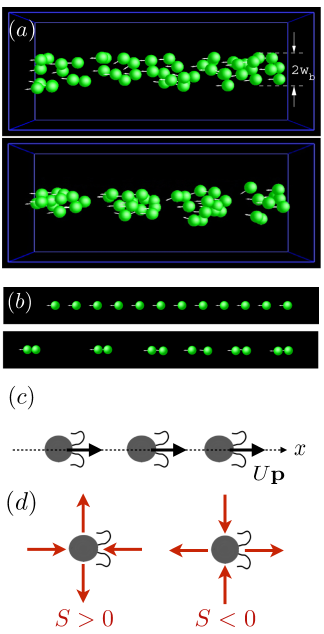
Figure 1: (a) Clustering instability of phototactic algae from numerical simulations as main motivation for our work jibuti14 ; (b) Similar instability arising on a one-dimensional line of swimming algae, which is the precise setup considered in this paper. Reproduced from Jibuti et al. (2014) Phys. Rev. E, 90. Copyright 2014, American Physical Society; (c) Sketch of the model problem addressed in this paper: a one-dimensional line of swimmers of fixed orientation ${\bf p}={\bf e}_{x}$ swimming with identical speed $U$ in the absence of rotational diffusion; (d) each swimmer acts on the fluid as a stresslet of magnitude $S$, creating in the swimming frame local flows as illustrated by solid red arrows.

As a simple starting point to understand these instabilities, we consider in this paper the problem of an initially homogeneous one-dimensional line of aligned swimmers moving along the same direction. We ignore rotational diffusion (except in the introduction section where the standard theoretical framework is summarised) and therefore the swimmers remain aligned, while their one-dimensional density is allowed to vary. We characterise analytically density instabilities using two complementary modelling approaches, namely a continuum framework and a discrete, point-swimmer, framework. In both cases we show that hydrodynamic interactions between the swimmers are responsible for the clustering and compute the growth rate of the instability. Both approaches give the same results and indicate that the instability arises only for puller-type swimmers such as the algae considered in Ref. jibuti14 while pushers are predicted to remain stable.

II Continuum framework

In the first approach, we use the classical continuum framework for suspension of swimming cells simha02 ; saintillan13 . The suspension is characterised by a probability distribution function, $\Psi({\bf r},{\bf p},t)$, for the position ${\bf r}$ and orientation ${\bf p}$ of the cells. Conservation of probability is written as

$$\frac{{\partial}\Psi}{{\partial}t}+\nabla_{\bf r}\cdot(\dot{\bf r}\Psi)+\nabla_{\bf p}\cdot(\dot{\bf p}\Psi)=D\nabla_{\bf r}^{2}\Psi+D_{R}\nabla_{\bf p}^{2}\Psi,$$ (1)

where $D$ is a diffusion constant in position and $D_{R}$ in orientation. The swimmers self-propel with speed $U$ along their direction ${\bf p}$ (Fig. 1c) and are also advected by the flow ${\bf u}$ and thus we have the relationship

$$\dot{\bf r}=U{\bf p}+{\bf u}.$$ (2)

The velocity field ${\bf u}$ is incompressible, $\nabla_{\bf r}\cdot{\bf u}=0$, and satisfies Stokes equation with a pressure field $q$

$$-\nabla_{\bf r}q+\mu\nabla_{\bf r}^{2}{\bf u}+\nabla_{\bf r}\cdot\boldsymbol{\Sigma}={\bf 0},$$ (3)

the last term being the active stress due to the active particles, namely the stresslet

$$\boldsymbol{\Sigma}=S\left\langle{\bf p}{\bf p}-\frac{1}{3}{\bf 1}\right\rangle,$$ (4)

where the brackets $\langle\cdot\rangle$ denote orientational average i.e.

$$\langle\cdot\rangle\equiv\int\Psi(.){\rm d}{\bf p}.$$ (5)

In Eq. (4), the sign of the stresslet strength, $S$, plays an important role in collective dynamics: $S<0$ for pushers and $S>0$ for pullers (see illustration in Fig. 1d).

In the simulation of Ref. jibuti14 , the swimmers are phototactic and their swimming orientation is identical and aligned with the line of swimmers. We thus assume here that the swimmers are located on a single line, along the $x$ direction, and that their orientation is fixed and also along $x$. We thus look for solutions of the form

$$\Psi=\delta(y)\delta(z)\lambda(x,t)\delta({\bf p}-{\bf e}_{x}),$$ (6)

where $\lambda$ is the one-dimensional density of swimmers along the $x$ axis. Note that for the particular solution of the form of Eq. (6) to be admissible, we ignore diffusion in orientation in what follows as well as diffusion in position in the directions perpendicular to the axis $x$. Given the fixed orientation, the active stress is given by

$$\boldsymbol{\Sigma}=S\int\Psi\left({\bf e}_{x}{\bf e}_{x}-\frac{1}{3}{\bf 1}\right){\rm d}{\bf p},$$ (7)

which, using Eq. (6), becomes

$$\boldsymbol{\Sigma}=S\delta(y)\delta(z)\lambda(x,t)\left({\bf e}_{x}{\bf e}_{x}-\frac{1}{3}{\bf 1}\right).$$ (8)

The flow equation becomes

$$\frac{{\partial}q}{{\partial}x} = \mu\nabla^{2}u_{x}+\frac{2}{3}S\frac{{\partial}}{{\partial}x}\left[\delta(y)\delta(z)\lambda(x,t)\right],$$ (9)

$$\frac{{\partial}q}{{\partial}y} = \mu\nabla^{2}u_{y}-\frac{1}{3}S\frac{{\partial}}{{\partial}y}\left[\delta(y)\delta(z)\lambda(x,t)\right],$$ (10)

$$\frac{{\partial}q}{{\partial}z} = \mu\nabla^{2}u_{z}-\frac{1}{3}S\frac{{\partial}}{{\partial}z}\left[\delta(y)\delta(z)\lambda(x,t)\right],$$ (11)

$$0 = \frac{{\partial}u_{x}}{{\partial}x}+\frac{{\partial}u_{y}}{{\partial}y}+\frac{{\partial}u_{z}}{{\partial}z}\cdot$$ (12)

In order to make progress, we use Fourier transforms defined for any function $\alpha({\bf x},t)$ of space and time as

$$\alpha({\bf x},t)=\frac{1}{(2\pi)^{3}}\int e^{i({\bf k}\cdot{\bf x})}\hat{\alpha}({\bf k},t){\rm d}{\bf k}.$$ (13)

We proceed by Fourier-transforming Eq. (9)-(12) in space leading to

$$ik_{x}\hat{q} = -\mu k^{2}\hat{u}_{x}+\frac{2}{3}Sik_{x}\hat{\lambda},$$ (14)

$$ik_{y}\hat{q} = -\mu k^{2}\hat{u}_{y}-\frac{1}{3}Sik_{y}\hat{\lambda},$$ (15)

$$ik_{z}\hat{q} = -\mu k^{2}\hat{u}_{z}-\frac{1}{3}Sik_{z}\hat{\lambda},$$ (16)

$$0 = {\bf k}\cdot\hat{\bf u}.$$ (17)

In order to determine the pressure we take the dot product of the ${\bf k}$ vector with the first three equations and exploit Eq. (17) to get

$$ik^{2}\hat{q}=Si\hat{\lambda}\left[\frac{2}{3}k_{x}^{2}-\frac{1}{3}(k_{y}^{2}+k_{z}^{2})\right]=Si\hat{\lambda}\left[k_{x}^{2}-\frac{1}{3}k^{2}\right].$$ (18)

Plugging Eq. (18) into Eq. (14) then leads to

$$i\frac{k_{x}}{k^{2}}S\hat{\lambda}\left[k_{x}^{2}-\frac{1}{3}k^{2}\right]=-\mu k^{2}\hat{u}_{x}+\frac{2}{3}Sik_{x}\hat{\lambda},$$ (19)

which can be solved for $\hat{u}_{x}$ as

$$\hat{u}_{x}=\frac{iS\hat{\lambda}}{\mu}\frac{k_{x}}{k^{2}}\left(1-\frac{k_{x}^{2}}{k^{2}}\right).$$ (20)

In order to close the stability calculation we finally need to write down conservation of swimmers along the line. In one dimension the conservation of swimmers is written as

$$\frac{\partial\lambda}{\partial t}+\frac{\partial}{\partial x}\left[(U+u_{x}|_{(x,0,0,t)})\lambda\right]=D\frac{\partial^{2}\lambda}{\partial x^{2}}\cdot$$ (21)

Note that using Fourier notation, we can see that

$$u_{x}|_{(x,0,0,t)}=\frac{1}{(2\pi)^{3}}\int e^{ik_{x}x}\hat{u}_{x}({\bf k},t){\rm d}{\bf k}.$$ (22)

The base case is a uniform distribution of swimmers, characterised by $\lambda(x,t)=\lambda_{0}$, so that $\hat{\lambda}=\lambda_{0}\delta(k_{x})$. Note that $\lambda_{0}$ is the inverse of the initial inter-swimmer distance, which we denote $\Delta$ in what follows. From Eq. (22) and using Eq. (20) we thus see that

$$u_{x}|_{(x,0,0,t)}=\int e^{ik_{x}x}\frac{iS\lambda_{0}\delta(k_{x})}{\mu}\left(\frac{k_{x}}{k^{2}}-\frac{k_{x}^{3}}{k^{4}}\right){\rm d}{\bf k}=0,$$ (23)

and therefore the uniform concentration is indeed a base state.

We then consider perturbations of this case state, written as $\lambda(x,t)=\lambda_{0}+\lambda^{\prime}$, $u_{x}=u_{x}^{\prime}$. The linearisation of Eq. (21) around the base state gives

$$\frac{\partial\lambda^{\prime}}{\partial t}+U\frac{\partial\lambda^{\prime}}{\partial x}+\lambda_{0}\frac{\partial}{\partial x}\left[u_{x}^{\prime}|_{(x,0,0,t)}\right]=D\frac{\partial^{2}\lambda^{\prime}}{\partial x^{2}}\cdot$$ (24)

To get a self contained equation for $\lambda^{\prime}$ we then use the definition of the Fourier integral and rewrite it as

$$\frac{\partial\lambda^{\prime}}{\partial t}+U\frac{\partial\lambda^{\prime}}{\partial x}+i\frac{\lambda_{0}k_{x}}{(2\pi)^{3}}\int e^{ik_{x}x}\hat{u}^{\prime}_{x}({\bf k},t){\rm d}{\bf k}=D\frac{\partial^{2}\lambda^{\prime}}{\partial x^{2}}\cdot$$ (25)

Fourier transforming along the $x$ direction gives

$$\frac{\partial\hat{\lambda}^{\prime}}{\partial t}+Uik_{x}\hat{\lambda}^{\prime}+\frac{i\lambda_{0}k_{x}}{(2\pi)^{2}}\int\hat{u}^{\prime}_{x}({\bf k},t){\rm d}k_{y}{\rm d}k_{z}=-Dk_{x}^{2}\hat{\lambda}^{\prime}.$$ (26)

and then using Eq. (20) leads to the final stability relationship

$$\frac{\partial\hat{\lambda}^{\prime}}{\partial t}+Uik_{x}\hat{\lambda}^{\prime}=\frac{Sk_{x}^{2}\lambda_{0}\lambda^{\prime}}{\mu(2\pi)^{2}}\int\left(1-\frac{k_{x}^{2}}{k^{2}}\right)\frac{{\rm d}k_{y}{\rm d}k_{z}}{k^{2}}-Dk_{x}^{2}\hat{\lambda}^{\prime}.$$ (27)

Looking for exponentially growing modes of the form $\hat{\lambda}^{\prime}(k_{x},t)=f(k_{x})e^{\sigma t}$ and we find a dispersion relation

$$\sigma=-iUk_{x}+\frac{Sk_{x}^{2}\lambda_{0}}{\mu(2\pi)^{2}}\int\left(1-\frac{k_{x}^{2}}{k^{2}}\right)\frac{{\rm d}k_{y}{\rm d}k_{z}}{k^{2}}-Dk_{x}^{2}.$$ (28)

This dispersion relationship has three terms. The first is a pure traveling mode reflecting the fact that we are in the laboratory frame while the swimmers move with speed $U$. The third term is diffusive and stabilizing. In contrast, the second term is the one arising from hydrodynamic interactions and is the one leading to instabilities.

We can evaluate the integral in the second term of Eq. (28) using cylindrical coordinates, writing $k_{\perp}^{2}=k_{y}^{2}+k_{z}^{2}$, which yields

$$I=\int\frac{1}{k^{2}}\left(1-\frac{k_{x}^{2}}{k^{2}}\right) {\rm d}k_{y}{\rm d}k_{z}=2\pi\int_{k_{\mbox{\tiny min}}}^{k_{\mbox{\tiny max}}}\!\!\!\!\frac{k_{\perp}^{3}}{(k_{\perp}^{2}+k_{x}^{2})^{2}}{\rm d}k_{\perp},$$ (29)

where the bounds $k_{\mbox{\tiny min}}$ and $k_{\mbox{\tiny max}}$ of the second integral must be specified. We assume for simplicity that the swimmers move in an unbounded space such that the lower bound $k_{\mbox{\tiny min}}$ can be taken equal to zero. The upper bound needs to scale with $\Delta^{-1}$ since below the length scale $\Delta$ the continuous approach loses its meaning; for simplicity we take it here to be $k_{\mbox{\tiny max}}=\Delta^{-1}$ and making a different choice of the form $k_{\mbox{\tiny max}}=\alpha\Delta^{-1}$ does not affect the main results below.

The integral in Eq. (29) can then be calculated exactly and one finds

$$\sigma=-iUk_{x}+\frac{1}{4\pi}\frac{Sk_{x}^{2}}{\Delta\mu}\,f(k_{x}\Delta)-Dk_{x}^{2},$$ (30)

where the function $f$ is given by

$$f(u)\equiv-\left[\ln\left(\frac{u^{2}}{1+u^{2}}\right)+\frac{1}{1+u^{2}}\right].$$ (31)

To capture the instability, we need to consider only the real part, $\sigma_{R}$, of the right-hand side of Eq. (30), i.e. its last two terms. At small wavenumbers, i.e. for wavelength much larger than the initial (mean) distance between swimmers $k_{x}\Delta\ll 1$, the real part of the growth rate scales as

$$\sigma_{R}(k_{x})\sim-\frac{1}{2\pi}\frac{S}{\mu\Delta^{3}}(k_{x}\Delta)^{2}\ln(k_{x}\Delta),$$ (32)

and diffusion plays no role. A similar result will be obtained below with a discrete approach.

As can be seen from Eq. (32), in the case of puller cells with $S>0$, since the $\log$ term is negative, the real part of the growth rate is positive, and long wavelengths are unconditionally unstable. As discussed below, when considering practical situations of real microscopic swimmers, small wavelengths are also unstable, and thus a whole band of wavelengths $[0,\Delta^{-1}]$ is unstable, a result in line with Jibuti’s simulationsjibuti14 . Conversely, for negative values of $S$, so-called pusher cells, the growth rate is always negative and the system is always stable, also in agreement with Jibuti’s results.

III Discrete framework

We now consider a second, complementary, modelling approach for the same problem.

Specifically, we model the three-dimensional swimmers as discrete moving stresslets located on a uniform one-dimensional lattice of spacing $\Delta$. Due to the long range nature of the hydrodynamic interactions, we include the flow created by all other swimmers when computing the velocity of a given swimmer. The swimmers are equally spaced on the $x$ axis and we wish to assess the stability of such a situation. In the reference frame moving with speed $U$ along the $x$ axis, the swimmers are motionless if the situation is unperturbed. We then subject the homogenous line to a harmonic perturbation of wavenumber $k_{x}=2\pi/(p\Delta)$, where $p$ a positive integer, such that each individual swimmer is shifted from its equilibrium position by a small quantity $\epsilon_{n}\equiv\varepsilon\,\cos(k_{x}\,n\Delta)=\varepsilon\,\cos(2\pi n/p)$ (see notation in Fig. 2). Since the wavelength of the perturbation needs to be larger than $2\Delta$, the wavevector is bounded by $\pi/\Delta$.

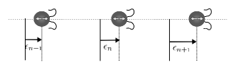
Figure 2: Discrete homogeneous one-dimensional line of swimmers. In the frame moving with the swimming speed of the cells, the perturbation distance to the equilibrium steady position of each swimming, $x_{n}$, is denoted $\epsilon_{n}$.

A swimmer located at ${\bf r}_{\scriptscriptstyle{0}}$ generates its own flow given by a force dipole

$$\mbox{\boldmath$u$}^{d}({\bf r}-{\bf r}_{\scriptscriptstyle{0}})=\mbox{\boldmath$S$}({\bf p})\colon\!\!\mbox{\boldmath$\nabla$}\mbox{\boldmath$\mathcal{G}$}({\bf r}-{\bf r}_{\scriptscriptstyle{0}}),$$ (33)

where $\mbox{\boldmath$S$}({\bf p})=S\,{\bf p}{\bf p}$ and $\mbox{\boldmath$\mathcal{G}$}({\bf r})=({\bf 1}+{\bf r}{\bf r})/8\pi\mu r$ is the stokeslet (point force) solution. All the dipoles have the same fixed orientation and subject to the flow generated on the $x$-axis ($y=z=0$) by all other swimmers. The $x$-component of the velocity field, Eq. (33), reduces to

$$u^{d}(x-x_{\scriptscriptstyle{0}})=-\frac{S}{4\pi\mu}\frac{x-x_{\scriptscriptstyle{0}}}{|x-x_{\scriptscriptstyle{0}}|^{3}}\cdot$$ (34)

In the absence of inertia, the dynamics of swimmer #$n$ is governed by the evolution of its perturbation, away from the equilibrium position, $\epsilon_{n}$, which follows thus

$$\dot{\epsilon}_{n}=\sum_{q>1}\left[u^{d}(x_{n}-x_{n-q})+u^{d}(x_{n}-x_{n+q})\right],$$ (35)

where the infinite sum includes interactions with all swimmers. The first term on the right-hand side of Eq. (35) can be expanded to first order in $\epsilon_{n}-\epsilon_{n-q}$ since $x_{n}-x_{n-q}=\Delta+\epsilon_{n}-\epsilon_{n-q}$ with $(\epsilon_{n}-\epsilon_{n-q})/\Delta\ll 1$, and one gets at first order

$$u^{d}(x_{n}-x_{n-q})=-\frac{S}{4\pi\mu}(q\Delta)^{-2}\left(1-2\frac{\epsilon_{n}-\epsilon_{n-q}}{q\Delta}\right),$$ (36)

with a similar result for $u^{d}(x_{n}-x_{n+q})$. Introducing these expansions in Eq. (35) leads to the equation which governs the evolution of the $\epsilon_{n}$ in time,

$$\dot{\epsilon}_{n}=-\frac{S}{4\pi\mu}\sum_{q>1}\frac{1}{(q\Delta)^{3}}(\epsilon_{n+q}+\epsilon_{n-q}-2\epsilon_{n}).$$ (37)

Note that this equation is valid in both the laboratory frame or the frame moving with the swimming speed $U$.

The perturbation in displacement $\epsilon_{n}$ (which “follows” the global displacement of the assembly at speed $U$) can be considered as a propagative wave in the laboratory frame, so that we consider a discrete perturbation of the form

$$\epsilon_{n\pm q}=\varepsilon\,\mbox{e}^{\tilde{\sigma}t}\mbox{e}^{-\mbox{\scriptsize i}[k_{x}(n\pm q)\Delta-\omega t)]},\;\;\mbox{with}\;\omega=k_{x}U.$$ (38)

When introduced in Eq. (37), this leads to the dispersion relationship which provides the discrete growth rate $\tilde{\sigma}(k_{x})$, and one finds the infinite sum

$$\tilde{\sigma}(k_{x})=-\mbox{i}Uk_{x}+\frac{2}{\pi}\frac{S}{\mu\Delta^{3}}\,\sum_{q>1}\frac{\sin^{2}(qk_{x}\Delta/2)}{q^{3}}\cdot$$ (39)

Here again, we see clearly from Eq. (39) that if $S<0$ (pushers) the system is predicted to be stable while a line suspension of pullers ($S>0$) is always unstable.

To address the behaviour at long wavelengths, we rewrite the real part $\tilde{\sigma}_{R}$ of the discrete growth rate, second term in the right-hand side of Eq. (39), in the following form

$$\tilde{\sigma}_{R}(k_{x})=\frac{1}{2\pi}\frac{S}{\mu\Delta^{3}}(k_{x}\Delta)^{2}\,\sum_{q>1}\frac{\sin^{2}(qk_{x}\Delta/2)}{(qk_{x}\Delta/2)^{3}}\,\frac{k_{x}\Delta}{2}.$$ (40)

The sum in Eq. (40), which has the form of a discrete integral, is bounded as follow

$$\int_{k_{x}\Delta/2}^{\infty}\!\!\frac{\sin^{2}u}{u^{3}}\,du <$$

$$\sum_{q>1} \frac{\sin^{2}(qk_{x}\Delta/2)}{(qk_{x}\Delta/2)^{3}}\,\frac{k_{x}\Delta}{2}$$

$$<\mbox{sinc}^{2}(k_{x}\Delta/2)+\int_{\bar{k}_{x}/2}^{\infty}\!\!\frac{\sin^{2}u}{u^{3}}\,du.$$ (41)

Given that the integral in both right and left bounds of the previous double inequality scales as $-\ln k_{x}\Delta$ for $k_{x}\Delta\rightarrow 0$, one obtains the scaling of $\sigma_{R}$ at small wavenumbers, namely

$$\tilde{\sigma}_{R}(k_{x})\sim-\frac{1}{2\pi}\frac{S}{\mu\Delta^{3}}(k_{x}\Delta)^{2}\ln(k_{x}\Delta),$$ (42)

which is exactly the same relationship as the one obtained in the continuum limit, Eq. (32).

.

IV Discussion

The spatial organisation of active matter under the combined effects of external Poiseuille flows and physical taxis (such as magnetotaxis or phototaxis) has been the subject of recent numerical and experimental studies jibuti14 ; Waisbord2016 ; Martin2016 . The interplay between hydrodynamic effects and physical taxis classically results in a focusing of the swimmers close to the axis of the channel pedley92 , the radial density profile being determined by the competition between the swimming-enhanced diffusivity of the swimmers and the amplitudes of external forcing.

In this paper, we examined theoretically the linear stability of swimmers along a one-dimensional clusters from both a continuum and discrete perspectives. The continuum approach, performed in Fourier space, leads to a stability condition involving two competing terms coming from hydrodynamic interactions and diffusion, respectively.

At small $k_{x}\Delta$, both modelling approaches provide a real part of the growth rate scaling as $\sigma_{R}(k_{x})\sim-(1/2\pi)[S/(\mu\Delta^{3})](k_{x}\Delta)^{2}\ln(k_{x}\Delta)$. In this limit diffusion plays no role – a result is in fact true, with very good approximation, for all wavenumbers. To see this, we take $D/\Delta^{2}$ as a typical timescale and denoting $\bar{k}_{x}$ the dimensionless product $k_{x}\Delta$, the real part $\sigma_{R}$ of the growth rate obtained in the continuum limit can be rewritten in the following dimensionless form

$$\bar{\sigma}_{R}(\bar{k}_{x})=\bar{k}_{x}^{2}\left[\bar{S}\,f(\bar{k}_{x})-1\right],$$ (43)

where $\bar{\sigma}_{R}=\Delta^{2}\sigma_{R}/D$ and $\bar{S}=(1/4\pi)[S/(D\Delta\mu)]$. For microscopic swimmers of size $a=1$ $\mu$m separated by an initial distance $\Delta/a=2$ and propelled in water ($\mu=10^{-3}$ Pa.s) by an individual stresslet of $S=1$ pN.$\mu$m, and writing $D\mu=k_{B}T/6\pi a$ where $k_{B}$ and $T$ refer to the Boltzmann constant and the temperature (300 K), one obtains the dimensionless value $\bar{S}\simeq 181$. Given the typical value of the dimensionless function $f$, one obtains that the diffusive term in Eq. (43) can basically always be neglected and with a good approximation we can write

$$\sigma_{R}(k_{x})\simeq\frac{1}{4\pi}\frac{S}{\mu\Delta^{3}}\,(k_{x}\Delta)^{2}\,f(k_{x}\Delta).$$ (44)

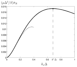
Figure 3: Dimensionless real part of the growth rate as a function of the dimensionless wave number, in the large $\bar{S}$ limit, Eq. (44). The dashed lines correspond to the improved small $k_{x}\Delta$ scaling $\sigma_{R}(k_{x})\simeq-(1/2\pi)[S/(\mu\Delta^{3})](k_{x}\Delta)^{2}\,[\ln(k_{x}\Delta)+1/2]$ obtained by taking into account the constant in the Taylor expansion of the function $f$.

The real part of the growth rate, non-dimensionalised as $S/(\mu\Delta^{3})$, is plotted in the large $\bar{S}$ limit (where diffusion is negligible) as a function of the dimensionless axial wavenumber, $k_{x}\Delta$, in Fig. 3, for positive values of the stresslet strength $S$ (i.e. in the unstable case of pullers). All wavelengths $k_{x}\Delta\in[0,1]$ are seen to be unstable. Furthermore, a most unstable wavelength $k^{\star}\Delta\approx 0.68$ is obtained. Considering however the small difference between the growth rate at $k^{\star}\Delta$ and at $k_{x}\Delta=1$, no real emergence of the most unstable wave length $\lambda^{\star}=2\pi/k^{\star}$ should be expected experimentally. This is consistent with the “pairing” scenario depicted in Jibuti et al. jibuti14 . It is likely that this pairing would continue in sequence, with swimmer pairs, which also act at pullers, pairing up, eventually leading to one big cluster.

The physical mechanism leading to the instability captured in our paper is in fact quite elementary, and can be captured by considering the line of swimmers sketched in Fig. 2. Puller cells induce attractive flows along their swimming axis with a magnitude which increases as one gets closer to the cell (Fig. 1d). In contrast, pushers induce repulsive flows, also with a magnitude increasing near the cell (Fig. 1d). Consider a situation where the location of the middle cell in Fig. 2 is perturbed to its right. If the cells are pushers, the repulsion with its neighbour on the right increases while the repulsion with the cell on the left decreases, and the cell returns to its original location, indicating stability. If in contrast the cells are pullers, the attraction toward the cell on the right increases, and the attraction with the left on the left decreases, leading to an amplification of the original perturbation, and an unstable situation. As a simple analogy, the instability of a line of pullers is thus similar to the instability of a line of point charges with alternating signs where while the periodic lattice is a fixed point, any perturbation to it is unstable.

While our theoretical predictions agree with the numerical results obtained in Ref. jibuti14 showing a jet instabilities for pullers in the absence of diffusion, we note that in contrast a recent experimental realisation of focused puller suspensions (specifically, the green alga Chlamydomonas) did not display such axial clustering Martin2016 . The origin of this discrepancy could for instance come from the existence of a threshold in flow intensity such as the one observed in Ref. Waisbord2016 for magnetotactic focusing. Indeed the jet pearling transition in Ref. Waisbord2016 was obtained as soon as the value of the flow intensity exceeds a critical value (for a fixed external magnetic field). Another possible source of discrepancy could come from our assumption to model the swimmer as a steady puller. Chlamydomonas is a puller on average but in fact oscillates between instantaneous pusher and puller behaviours klindt15 , potentially interfering with the development of an instability.

A simple extension of the situation considered in the present paper would be a configuration in which the direction of swimming is perpendicular to the line of swimmers. In this case, one expects pushers to be unstable while pullers would remain stable. An other extension would focus an axisymmetric situation in which a cylindrical blob of co-swimmers could be perturbed, or multiple parallel lines of swimmers. Such analysis would be closer to the experiment in Ref. Waisbord2016 and would be a step further towards the full modelling of instabilities of convected active suspensions subject to physical taxis.

This work was funded in part by the European Union through a Marie Curie CIG Grant and an ERC consolidator grant to EL.

References

- [1] S. Ramaswamy. The mechanics and statistics of active matter. Annu. Rev. Cond. Mat. Phys., 1:323–345, 2010.
- [2] E. Lauga and T. R. Powers. The hydrodynamics of swimming microorganisms. Rep. Prog. Phys., 72:096601, 2009.
- [3] M. C. Marchetti, J. F. Joanny, S. Ramaswamy, T. B. Liverpool, J. Prost, M. Rao, and R A. Simha. Hydrodynamics of soft active matter. Rev. Mod. Phys., 85:1143, 2013.
- [4] R. A. Simha and S. Ramaswamy. Hydrodynamic fluctuations and instabilities in ordered suspensions of self-propelled particles. Phys. Rev. Lett., 89:058101, 2002.
- [5] D. Saintillan and M. J. Shelley. Orientational order and instabilities in suspensions of self-locomoting rods. Phys. Rev. Lett., 99:058102, 2007.
- [6] D. Saintillan and M. J. Shelley. Instabilities and pattern formation in active particle suspensions: Kinetic theory and continuum simulations. Phys. Rev. Lett., 100:178103, 2008.
- [7] C. Hohenegger and M. J. Shelley. Stability of active suspensions. Phys. Rev. E, 81:046311, 2010.
- [8] D. L. Koch and G. Subramanian. Collective hydrodynamics of swimming microorganisms: Living fluids. Annu. Rev. Fluid Mech., 43:637 – 659, 2011.
- [9] J. P. Hernandez-Ortiz, C. G. Stoltz, and M. D. Graham. Transport and collective dynamics in suspensions of confined swimming particles. Phys. Rev. Lett., 95:204501, 2005.
- [10] A. Sokolov and I. S. Aranson. Physical properties of collective motion in suspensions of bacteria. Phys. Rev. Lett., 109:248109, 2012.
- [11] X. L. Wu and A. Libchaber. Particle diffusion in a quasi-two-dimensional bacterial bath. Phys. Rev. Lett., 84:3017–3020, 2000.
- [12] C. Valeriani, M. Li, J. Novosel, J. Arlt, and D. Marenduzzo. Colloids in a bacterial bath: simulations and experiments. Soft Matt., 7(11):5228–5238, 2011.
- [13] A. Jepson, V. A. Martinez, J. Schwarz-Linek, A. Morozov, and W. C. K. Poon. Enhanced diffusion of nonswimmers in a three-dimensional bath of motile bacteria. Phys. Rev. E, 88:041002, 2013.
- [14] T. V. Kasyap, D. L. Koch, and M. Wu. Hydrodynamic tracer diffusion in suspensions of swimming bacteria. Phys. Fluids, 26:081901, 2014.
- [15] D. O. Pushkin and J. M. Yeomans. Fluid mixing by curved trajectories of microswimmers. Phys. Rev. Lett., 111(18):188101, 2013.
- [16] D. T. N. Chen, A. W. C. Lau, L. A. Hough, M. F. Islam, M. Goulian, T. C. Lubensky, and A. G. Yodh. Fluctuations and rheology in active bacterial suspensions. Phys. Rev. Lett., 99(14):148302, 2007.
- [17] A. Sokolov and I. S. Aranson. Reduction of viscosity in suspension of swimming bacteria. Phys. Rev. Lett., 103:148101, 2009.
- [18] A. Sokolov, M. M. Apodaca, B. A. Grzybowski, and I. S. Aranson. Swimming bacteria power microscopic gears. Proc. Natl. Acad. Sci. USA, 107:969–974, 2010.
- [19] T. J. Pedley and J. O. Kessler. Hydrodynamic phenomena in suspensions of swimming microorganisms. Annu. Rev. Fluid Mech., 24:313–358, 1992.
- [20] L. Jibuti, L. Qi, C. Misbah, W. Zimmermann, S. Rafaï, and P. Peyla. Self-focusing and jet instability of a microswimmer suspension. Phys. Rev. E, 90:063019, 2014.
- [21] D Saintillan and M J. Shelley. Active suspensions and their nonlinear models. Comptes Rendus Phys., 14:497– 517, 2013.
- [22] N. Waisbord, C. Lefèvre, L. Bocquet, C. Ybert, and C. Cottin-Bizonne. Destabilization of a flow focused suspension of magnetotactic bacteria. Phys. Rev. Fluids, 1:053203, 2016.
- [23] M. Martin, A. Barzyk, E. bertin, P. Peyla, and S. Rafai. Photofocusing: Light and flow of photoactic microswimmer suspension. Phys. Rev. E, 93:051101, 2016.
- [24] G. S Klindt and B. M. Friedrich. Flagellar swimmers oscillate between pusher-and puller-type swimming. Phys. Rev. E, 92:063019, 2015.