Radiation from transmission lines PART I: free space transmission lines

Abstract

This work derives exact expressions for the radiation from two conductors non isolated TEM transmission lines of any cross section in free space. We cover the cases of infinite, semi-infinite and finite transmission lines and show that while an infinite transmission line does not radiate, there is a smooth transition between the radiation from a finite to a semi-infinite transmission line. Our analysis is in the frequency domain and we consider transmission lines carrying any combination of forward and backward waves. The analytic results are validated by successful comparison with ANSYS commercial software simulation results, and successful comparisons with other published results.

I Introduction

The aim of this work is to calculate the radiated power from two conductors transmission lines (TL) in free space. We consider any cross section of small electric size (shown in Figure 1) and TL of any length, analyzing the infinite, semi-infinite and finite TL cases. Part II is the generalization of this work for TL inside dielectric insulator and will be published separately. Some preliminary results of this work have been presented in [1, 2].

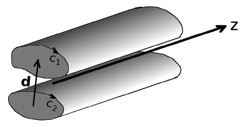
Figure 1: A basic configuration of a two ideal conductors TL, with a well defined separation between the conductors. The surface current distributions on the contours of the conductors is known from electrostatic considerations, and given that for a two-conductors TL there is only one (differential) TEM mode, the total current is the same on both conductors but with opposite signs. The arrow shows the vector distance between the center of the surface current distributions, named $\mathbf{d}$, obtained for a twin lead equivalent (see Appendix A). $c_{1,2}$ are the contours of the “upper” and “lower” conductors, respectively. We consider the case of small electric cross section $kd\ll 1$, $k$ is the wavenumber.

One of the earliest analysis of radiation from transmission lines (TL) is presented in the paper “Radiation from Transmission Lines” [3], published in 1923. In this publication the radiation from open ended twin lead TL in free space, at the resonance frequencies is calculated.

A more conclusive and full analysis is presented in the 1951 paper “Radiation Resistance of a Two-Wire Line” [4]. This work calculates the radiation resistance of a twin lead loaded at its termination by any impedance, considering TL ohmic losses as well. In this work we consider 0 ohmic losses, but generalize [4] as follows:

• We consider the separate radiation of the forward and backward waves and also their combination. From such analysis it comes out that the interference term between the waves does not contribute to the radiated power.

• We analyze the radiation from semi-infinite TL, and show the connection with the finite TL case.

• We do not limit ourselves to the twin lead cross section, and present a general algorithm for TL of any cross section.

• We develop a more accurate radiation resistance.

Additional works on the subject can be found in [5, 6, 7]. It is interesting to remark that [8] claims that balanced TL do not radiate. Although [8] is only an educational document of a university, such inaccuracy is a symptom showing that the subject of radiation from TL is not well enough known in the electromagnetic community, requiring additional research on this subject.

There are two appendices in this work. In Appendix A we calculate the far potential vector from a general cross section TL (see Figure 1), and show that this far potential vector can be represented in terms of an equivalent twin lead as shown in Figure 2. By “far” we mean in the transverse $x,y$ direction because this appendix is not limited to finite TL, so for being able to use the results for a semi-infinite TL, we keep everything in cylindrical coordinates, and consider the TL between $z_{1}$

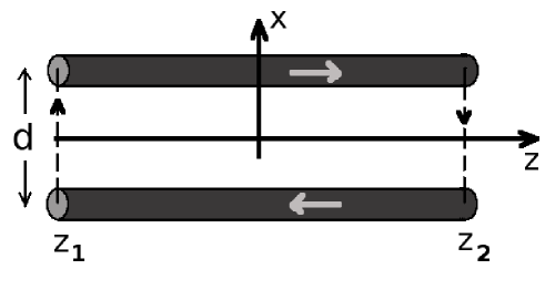
Figure 2: The transmission line is modeled as a twin lead in free space, with distance $d$ between the conductors. The currents in the transmission line flow in the $z$ direction at $x=\pm d/2$ and they contribute to the magnetic vector potential $A_{z}$. The termination currents (source or load) flow in the $x$ direction and contribute the magnetic vector potential $A_{x}$. The arrows on the conductors show the conventional directions of those currents. The wires appear in the figure with finite thickness, but are considered of 0 radius. The transmission line goes in the $z$ direction from $z_{1}$ to $z_{2}$.

and $z_{2}$ on the $z$ axis. The twin lead model is defined without loss of generality on the $x,z$ plane and allows us to define $x$ directed termination currents as current filaments [4] across the termination (see Figure 2). Those termination currents contribute a far $x$ directed potential vector, calculated in Appendix A.

In Appendix B we show how to calculate for any cross section the parameters needed to determine the radiation: the separation distance $d$ in the twin lead representation, and the characteristic impedance $Z_{0}$. We perform this analysis on two cross section examples.

It is important to remark that the calculations in this work and in [4, 3, 5, 6, 7] are completely different from what is presented as “traveling wave antenna” in many antenna and electromagnetic books like [9, 10, 11, 12, 13]. The last ones consider only the current in the “upper” conductor in Figure 2, while we consider all 4 currents appearing in the figure. This is not an attempt to criticize those works, but only to mention their results do not represent radiation from transmission lines, hence are not comparable with the results of this work or [4, 3, 5, 6, 7].

It should be also mentioned that power loss from TL is also affected by nearby objects interfering with the fields, line bends, irregularities, etc. This is certainly true, but those affect not only the radiation, but also the basic, “ideal” TL model in what concerns the characteristic impedance, the propagation wave number, etc. Those non-ideal phenomena are not considered in the current work, nor in [4, 3, 5, 6, 7], and also not in [9, 10, 11, 12, 13].

The methodology we use for calculating radiation losses is first order perturbation: we use the lossless (0’th order solution) for the electric current to derive the losses, and we therefore use in Appendix A the $e^{-jkz}$ dependence. This methodology is used to derive the ohmic and dielectric losses [14, 10, 11, 12], and the same approach is used in different radiation schemes from free electrons: one uses the 0’th order current (which is unaffected by the radiation) to calculate the radiation [17, 18, 19]. To be mentioned that the same approach has been used in [4, 3, 5, 6, 7] (although [4] discussed about higher order terms, without applying them).

The main text is organized as follows. In Section II we use the results of Appendix A to calculate the power radiated from a finite TL carrying a forward wave current, and generalize this result for any combination of waves. As mentioned earlier, the results of Appendix A are applicable also for semi-infinite TL, but we prefer to start with the finite TL, because in the following Section III we validate the analytic results of Section II by comparing them with ANSYS commercial software simulation results, and with published results obtained by other authors.

Section IV we base on Appendix A to analyze an infinite and semi-infinite TL. As expected, an infinite TL does not radiate and rather carries power in the $z$ direction only, but a semi-infinite TL does radiate, and we show in this section the connection between the finite and semi-infinite case and how the transition between them occurs. Here, it is important to mention that in some senses a finite matched TL is very similar to an infinite TL: in both cases there is no reflected wave, but they are very different in what concerns radiation: the first radiates and the second does not.

In Section V we discuss the radiation resistance and generalize the formula derived in [4].

The work is ended with some concluding remarks.

Note: through this work, the phasor amplitudes are RMS values, hence there is no 1/2 in the expressions for power. Also, it is worthwhile to mention that the results of this work depend on physical sizes relative to the wavelength, and hence are valid for all frequencies.

II Power radiated from a finite TL

II-A Matched TL

We calculate in this subsection the power radiated form a TL of length $2L$, carrying a forward wave, represented by the current

$$I(z)=I^{+}e^{-jkz}$$ (1)

We set $z_{1}=-L$ and $z_{2}=L$ in the expression for the $z$ directed magnetic vector potential in Eq. (A.13) from Appendix A, and obtain in spherical coordinates:

$$A_{z}=\mu_{0}G(r)F_{(z)}(\theta,\varphi)$$ (2)

where $G$ is the 3D Green’s function defined in (Eq. (A.2)), and

$$F_{(z)}(\theta,\varphi)=jI^{+}2Lkd\sin\theta\cos\varphi\operatorname{sinc}\left[kL(1-\cos\theta)\right]$$ (3)

is the directivity function, and the subscript $(z)$ denotes the contribution from the $z$ directed currents. The sinc function is defined $\operatorname{sinc}(x)\equiv\sin x/x$. To obtain the far fields (those decaying like $1/r$), the $\boldsymbol{\nabla}$ operator is approximated by $-jk\mathbf{\widehat{r}}$ and one obtains:

$$\mathbf{H}_{(z)}=\frac{1}{\mu_{0}}\boldsymbol{\nabla}\times(A_{z}\mathbf{\widehat{z}})=jkG(r)F_{(z)}(\theta,\varphi)\sin\theta\boldsymbol{\widehat{\varphi}}$$ (4)

and $\mathbf{E}_{(z)}=\eta_{0}\mathbf{H}_{(z)}\times\mathbf{\widehat{r}}$, where $\eta_{0}=\sqrt{\mu_{0}/\epsilon_{0}}=120\pi\,\Omega$ is the free space impedance. For the contribution of the $x$ directed end currents we sum the results for the $x$ directed magnetic vector potential from Eq. (A.16) in Appendix A (setting $z_{1}=-L$ and $z_{2}=L$), obtaining

$$A_{x}=\mu_{0}G(r)F_{(x)}(\theta,\varphi)$$ (5)

where

$$F_{(x)}(\theta,\varphi)=2jI^{+}d\sin\left[kL(1-\cos\theta)\right]$$ (6)

is the directivity function, and the subscript $(x)$ denotes the contribution from the $x$ directed currents. The fields from the $x$ directed end currents are calculated, obtaining

$$\mathbf{H}_{(x)}=\frac{1}{\mu_{0}}\boldsymbol{\nabla}\times(A_{x}\mathbf{\widehat{x}})=-jkG(r)F_{(x)}(\cos\theta\cos\varphi\boldsymbol{\widehat{\varphi}}+\sin\varphi\boldsymbol{\widehat{\theta}})$$ (7)

and $\mathbf{E}_{(x)}=\eta_{0}\mathbf{H}_{(x)}\times\mathbf{\widehat{r}}$. Now summing the fields contributed by the $z$ directed currents with those contributed by the $x$ directed currents, we obtain $\mathbf{H}=\mathbf{H}_{(z)}+\mathbf{H}_{(x)}$:

$$\mathbf{H}=jkG(r)[\boldsymbol{\widehat{\varphi}}(F_{(z)}\sin\theta-F_{(x)}\cos\theta\cos\varphi)-\boldsymbol{\widehat{\theta}}F_{(x)}\sin\varphi].$$ (8)

Using Eqs (3) and (6), the explicit expression for the far magnetic field is

$$\mathbf{H}^{+}=-G(r)2kdI^{+}\sin\left[2kL\sin^{2}(\theta/2)\right][\boldsymbol{\widehat{\varphi}}\cos\varphi-\boldsymbol{\widehat{\theta}}\sin\varphi].$$ (9)

We now use the superscript + on all the quantities calculated in this subsection, to denote that they refer to a forward wave. The far electric field is

$$\mathbf{E}^{+}=\eta_{0}\mathbf{H}^{+}\times\mathbf{\widehat{r}}$$ (10)

We remark that the polarization of the fields is not well defined at $\theta=0$ (as shown in Figure 3), but this is not a problem in this case, because the fields are 0 at this point.

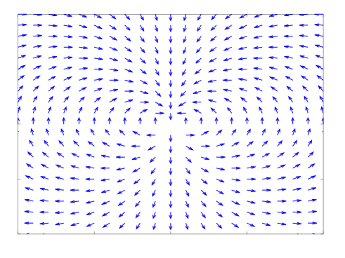
Figure 3: The polarization of the $H^{+}$ field $\boldsymbol{\widehat{\varphi}}\cos\varphi-\boldsymbol{\widehat{\theta}}\sin\varphi$ , according to Eqs. (9), around $\theta=0$ (“north pole”). The $z$ axis comes toward us from the center of the plot (at $\theta=0$), $\varphi$ is 0 at the right side and increases counterclockwise. The polarization is not defined at $\theta=0$, but the fields are 0 at this location.

The far Poynting vector $\mathbf{S}^{+}=\mathbf{E}^{+}\times\mathbf{H}^{+*}$ comes out

$$\mathbf{S}^{+}=\frac{\mathbf{\widehat{r}}\eta_{0}k^{2}d^{2}|I^{+}|^{2}}{4\pi^{2}r^{2}}\sin^{2}\left[2kL\sin^{2}(\theta/2)\right]$$ (11)

so that the total radiated power is calculated via

$$\int_{0}^{2\pi}\int_{0}^{\pi}\sin\theta d\theta d\varphi r^{2}\mathbf{\widehat{r}}\cdot\mathbf{S}.$$ (12)

and comes out

$$P_{rad}^{+}=60\,\Omega|I^{+}|^{2}(kd)^{2}\left[1-\operatorname{sinc}(4kL)\right].$$ (13)

The radiation pattern function is calculated from the radial pointing vector (Eq. 11) and the total power in Eq. (13): $D^{+}=4\pi r^{2}S_{r}^{+}/P_{rad}^{+}$, which comes out

$$D^{+}(\theta)=2\frac{\sin^{2}[2kL\sin^{2}(\theta/2)]}{\left[1-\operatorname{sinc}(4kL)\right]}.$$ (14)

The function $D^{+}$ is 0 for $\theta=0$, and its number of lobes increases as the TL length increases. A one dimensional plot of $D^{+}$ as function of $\theta$ for different TL lengths is shown in Figure 4.

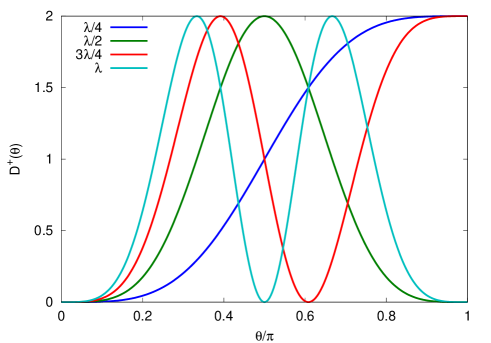
Figure 4: $D^{+}$ as function of $\theta$ for TL $2L=\lambda/4$, $\lambda/2$, $3\lambda/4$ and $\lambda$.

The radiated power relative to the forward wave propagating power ($P^{+}=|I^{+}|^{2}Z_{0}$) is given by

$$\frac{P_{rad}^{+}}{P^{+}}=\frac{60\,\Omega}{Z_{0}}(kd)^{2}\left[1-\operatorname{sinc}(4kL)\right],$$ (15)

As results from Eq. (15), the calculation of the relative radiated power requires the knowledge of two parameters: the separation distance in the twin lead representation $d$ (relative to the wavelength), and the characteristic impedance of the actual cross section $Z_{0}$, and in Appendix B we show examples of how to calculate this two parameters for different cross sections.

In the following subsection we generalize the radiation losses for a TL with any termination.

II-B Generalization for non matched line

We generalize here the result (13) obtained for the losses of a finite TL carrying a forward wave to any combination of waves, as follows:

$$I(z)=I^{+}e^{-jkz}+I^{-}e^{jkz}$$ (16)

where $I^{+}$ is the forward wave phasor current, as used in the previous subsection and $I^{-}$ is the backward wave phasor current, still defined to the right in the “upper” line in Figure 2.

The solution for a backward moving wave (only) on the finite TL, with a current phasor amplitude $I^{-}$ can be found by first solving for a reversed $z$ axis in Figure 2, i.e. a $z$ axis going to the left, replacing in the solution $I^{+}\rightarrow-I^{-}$. But this defines exactly the same configuration for the backward wave, as the original $z$ axis defined for a forward wave, hence resulting in the same solution in Eqs. (9) and (10). Now to express the solution for the backward wave in the original coordinates, defined by the right directed $z$ axis, one has to replace: $\theta\rightarrow\pi-\theta$, $\varphi\rightarrow-\varphi$, and therefore also $\boldsymbol{\widehat{\theta}}\rightarrow-\boldsymbol{\widehat{\theta}}$ and $\boldsymbol{\widehat{\varphi}}\rightarrow-\boldsymbol{\widehat{\varphi}}$. Hence, for a backward wave, the far H field is

$$\mathbf{H}^{-}=-G(r)2kdI^{-}\sin\left[2kL\cos^{2}(\theta/2)\right][\boldsymbol{\widehat{\varphi}}\cos\varphi+\boldsymbol{\widehat{\theta}}\sin\varphi],$$ (17)

so that the polarization at $\theta=\pi$ is not defined, and it looks like in Figure 3, this time the center of the plot is $\theta=\pi$, and $\varphi$ increases clockwise. Again, this is no problem because for this case the fields vanish at $\theta=\pi$.

For a backward wave only, the radiation pattern is:

$$D^{-}(\theta)=2\frac{\sin^{2}[2kL\cos^{2}(\theta/2)]}{\left[1-\operatorname{sinc}(4kL)\right]},$$ (18)

which looks like in Figure 4, only reflected around $\theta=\pi/2$.

We sum the fields of the forward and backward waves given in Eqs. (9) and (17), obtaining

$$\mathbf{H}=kG(r)2d$$

$$[-\boldsymbol{\widehat{\varphi}}\cos\varphi(I^{+}\sin\left[2kL\sin^{2}(\theta/2)\right]+I^{-}\sin\left[2kL\cos^{2}(\theta/2)\right])+$$

$$\boldsymbol{\widehat{\theta}}\sin\varphi(I^{+}\sin\left[2kL\sin^{2}(\theta/2)\right]-I^{-}\sin\left[2kL\cos^{2}(\theta/2)\right])],$$ (19)

so the far Poynting vector is

$$\mathbf{S}= \mathbf{\widehat{r}}\eta_{0}\frac{4(kd)^{2}}{16\pi^{2}r^{2}}\left\{|I^{+}|^{2}\sin^{2}\left[2kL\sin^{2}(\theta/2)\right]+|I^{-}|^{2}\right.$$

$$\sin^{2}\left[2kL\cos^{2}(\theta/2)\right]+2\cos(2\varphi)$$

$$\left.\sin\left[2kL\sin^{2}(\theta/2)\right]\sin\left[2kL\cos^{2}(\theta/2)\right]\Re\{I^{+}I^{-*}\}\right\}$$ (20)

The interference between the waves does not contribute to the radiated power (because $\int_{0}^{2\pi}d\varphi\cos(2\varphi)=0$). The radiated power comes out

$$P_{rad}= 60\,\Omega(kd)^{2}\left(|I^{+}|^{2}+|I^{-}|^{2}\right)\left[1-\operatorname{sinc}(4kL)\right]\equiv$$

$$P^{+}_{rad}+P^{-}_{rad},$$ (21)

where $P_{rad}^{+}$ is given in Eq. (13) and $P^{-}_{rad}$ is similar, only replace $I^{+}$ by $I^{-}$.

The radiation pattern for the general case of forward and backward waves is $D=4\pi r^{2}S_{r}/P_{rad}$, where $S_{r}$ is given in Eq. (20) and $P_{rad}$ in (21). To express $D$ independently of the currents, it is convenient to consider a general TL circuit in Figure 5,

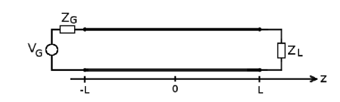
Figure 5: TL fed by a generator $V_{G}$ with an internal impedance $Z_{G}$, loaded by $Z_{L}$. The value of $Z_{L}$ affects indirectly the radiated power by setting the relation between the forward and backward currents $I^{+}$ and $I^{-}$.

for which the relation between $I^{+}$ and $I^{-}$ is

$$I^{-}e^{jkL}+\Gamma I^{+}e^{-jkL}=0,$$ (22)

where $\Gamma\equiv\frac{Z_{L}-Z_{0}}{Z_{L}+Z_{0}}$. Using (22), the radiation pattern is

$$D(\theta,\varphi)=2\frac{A^{2}+|\Gamma|^{2}B^{2}-2AB\cos(2\varphi)\Re\{\Gamma e^{-2jkL}\}}{\left(1+|\Gamma|^{2}\right)\left[1-\operatorname{sinc}(4kL)\right]},$$ (23)

where $A$ and $B$ are abbreviations for:

$$A\equiv\sin\left[2kL\sin^{2}(\theta/2)\right]\,\,\,B\equiv\sin\left[2kL\cos^{2}(\theta/2)\right]$$ (24)

For a matched TL, $\Gamma=0$, and Eq. (23) reduces to Eq. (14). We remark that although the interference between the forward and backward waves does not contribute to the radiated power (see Eq. 21), it distorts the radiation pattern and introduces a $\varphi$ dependence.

As mentioned in the introduction, the “traveling wave antenna” presented in [9, 10, 11, 12, 13] do not represent transmission lines, and therefore the radiation patterns in (14) or (23) are not comparable with those presented in the above references. They will be however compared with [6, 15, 16].

In the next section we validate the analytic results obtained in this section, using ANSYS commercial software simulation and additional published results on radiation losses from TL.

III Validation of the analytic results

III-A Comparison with ANSYS simulation results

We compare in this subsection the relative radiated power from a two-conductor TL (Eq. 15) carrying a forward wave, with the relative radiation losses results obtained from ANSYS commercial software simulation. For the comparison we use the cross section of two parallel cylinders, for which the analytic solution is known from image theory [14, 10, 11, 12], but also confirmed by Appendix B. The cross section is shown in Figure 6. The diameters of the cylinders are $2a=0.0203\lambda$, and the distance between their centers is $s=0.02872\lambda$, where the wavelength $\lambda=6.25$ cm, corresponding to the frequency of 4.8 GHz.

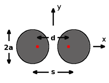
Figure 6: Cross section of two parallel cylinders: the distance between the centers is $s=0.02872$, and the diameters are $2a=0.0203$ wavelengths. The the red points show the current images which define the twin lead representation, and the distance between them $d=0.0203$ wavelengths is calculated in Eq. (25).

The distance between the image currents (shown as red points in Figure 6) is the separation distance $d$ in the twin lead model, given by

$$d=\sqrt{s^{2}-(2a)^{2}}=0.0203\lambda,$$ (25)

so that $(kd)^{2}=0.016$ is small enough, and the characteristic impedance is

$$Z_{0}=\frac{\eta_{0}}{\pi}\ln\left(\frac{d+s}{2a}\right)=105.6\,\Omega$$ (26)

Both analytic results for $d$ and $Z_{0}$ compare well with those calculated in Appendix B for this cross section.

We simulated the configuration in Figure 6 using ANSYS-HFSS commercial software, in the frequency domain, FEM technique. The box surface enclosing the device constitutes a radiation boundary, implying absorbing boundary conditions (ABC), used to simulate an open configuration that allows waves to radiate infinitely far into space. ANSYS HFSS ABC, absorbs the wave at the radiation boundary, essentially ballooning the boundary infinitely far away from the structure. The enclosing box surface has to be located at least a quarter wavelength from the radiating source. For the frequency of 4.8 GHz we used, the wavelength is 6.25 cm , and we chose the box sides 7.5 cm in the $x$ and $y$ directions, and the TL length plus 2.5 cm on each side in the $z$ direction. For the interface to the device we used lumped ports, which define perfect H boundaries everywhere on the port plane, so that the E field on the port plane (outside the conductors) is perpendicular to the conductors.

The simulation setup is shown schematically in Figure 7. The TL is ended at both sides by lumped ports of characteristic impedance $Z_{port}=50\,\Omega$, but fed only from port 1 by forward wave voltage $V^{+}_{port}=1\,V$, so the equivalent Thévenin feeding circuit is a generator of $2V^{+}_{port}$ in series with a resistance $Z_{port}$.

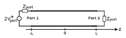
Figure 7: Simulation setup for obtaining $2\times 2$ S matrices for different TL lengths.

We obtained from the simulation S matrices defined for a characteristic impedance of $Z_{port}$ at both ports (which is an arbitrary choice), for different lengths of the transmission line. By symmetry, the S matrix has the form

$$S=\left(\begin{array}[]{cc}\Gamma&\tau\\ \tau&\Gamma\end{array}\right),$$ (27)

from which one may calculate the ABCD matrix of the TL [14, 20, 21, 22]. We need only the A element from the matrix:

$$A=\frac{1}{2}\left[\tau+(1-\Gamma^{2})/\tau\right]$$ (28)

from which we compute the delay angle (or electrical length) of the TL

$$\Theta=\arccos(A)$$ (29)

The real part of $\Theta$ represents the phase accumulated by a forward wave along the TL, and the imaginary part of $\Theta$ (which is always negative) represents the relative decay of the forward wave (voltage or current) due to losses (in our case there are only radiation losses) along the TL, so that $|I^{+}(L)|=|I^{+}(-L)|\exp(\text{Im}\{\Theta\})$. Therefore, the power carried by the forward wave $|P^{+}(L)|=|P^{+}(-L)|\exp(2\text{Im}\{\Theta\})$, but for small losses $|P^{+}(L)|\simeq|P^{+}(-L)|(1+2\text{Im}\{\Theta\})$, so that the difference between the input and output values of $P^{+}$ (which represent the radiated power $P_{rad}^{+}$ in Eq. (15)), relative to the (average) power $P^{+}$ carried by the wave is obtained by

$$\frac{P_{rad}^{+}}{P^{+}}=-2\text{Im}\{\Theta\},$$ (30)

where Im is the imaginary part and Im$\{\Theta\}<0$ always.

In Figure 8 and Table I we compare the analytic result in Eq. (15) with the result obtained from simulation Eq. (30), for a fixed frequency of 4.8 GHz and different TL lengths.

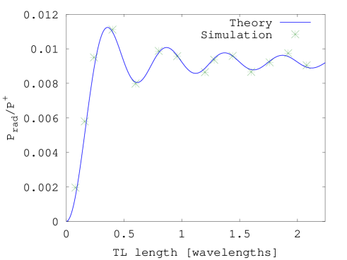
Figure 8: Relative radiation losses for a matched TL $P_{rad}/P^{+}$: comparison between the analytic result in Eq. (15) and the simulation result in Eq. (30) for different TL lengths in units of wavelengths.

TABLE I: The numerical data from Figure 8 and the relative error.

TL length	simulation (Eq. 30)	theoretical (Eq. 15)	% error
0.08	0.001963	0.001479	32.76
0.16	0.005796	0.005079	14.12
0.24	0.009502	0.008851	7.35
0.4	0.011115	0.010982	1.21
0.6	0.007987	0.008069	-1.02
0.8	0.009878	0.009774	1.06
0.96	0.009575	0.009603	-0.28
1.12	0.008198	0.008579	-4.44
1.2	0.008646	0.008874	-2.57
1.28	0.009366	0.009445	-0.84
1.44	0.009589	0.009583	0.05
1.6	0.008665	0.008797	-1.50
1.76	0.009216	0.009286	-0.75
1.92	0.009746	0.009557	1.98
2.08	0.009046	0.008936	1.23

We see that the simulation confirms well the theoretical result, with an average absolute relative error of 4.75%. The biggest relative errors are at the short TL, where the relative radiation losses are low, and hence more difficult to reproduce accurately with the simulation. For example, if we exclude the shortest TL length of 0.08$\lambda$ from the comparison, the average absolute relative error is 2.75%, or if we exclude the 2 shortest points of 0.08 and 0.16$\lambda$ from the comparison, it drops to 1.87%.

III-B Comparison with [3]

In 1923 Manneback [3] published a paper “Radiation from transmission lines” which calculated the power radiated by two thin wires of length $l$ (equivalent to our $2L$), and separation $d$, in resonance, having open terminations. The author considered the current

$$I_{m}\cos(k_{n}z)\sin(\omega_{n}t)$$ (31)

where $k_{n}=\pi n/l$ and $\omega_{n}=ck_{n}$ for odd $n$ (as defined in Eq. 3 of [3]). Note that the time dependence has been explicitly written in [3] and the calculations have been done in time domain, but using a fixed frequency, hence they are completely equivalent to our phasor calculations. The result for the radiated power is given in Eq. 11 of [3], rewritten here for convenience

$$P_{rad}=15\,\Omega(kd)^{2}I_{m}^{2}$$ (32)

We compare this with our result (21). $kl=n\pi$ is in our notation $kL=n\pi/2$ hence the sinc function in Eq. (21) results 0. This resonant case implies $I^{+}=I^{-}$, so the general current in Eq. (16) reduces to

$$2I^{+}\cos(kz)$$ (33)

and Eq. (21) results in $120\,\Omega(kd)^{2}|I^{+}|^{2}$.

The value $I_{m}$ in Eq. (31) is the amplitude of the current, i.e. the RMS value times $\sqrt{2}$. We use RMS values (as mentioned in the introduction) hence the equivalence between Eq. (31) and Eq. (33) is by setting $I_{m}=2\sqrt{2}|I^{+}|$, and using this equivalence, Eq. (21) reduces exactly to Eq. (32).

To be mentioned that our results are general, covering all cases of terminations, or any combination of waves, and we showed in this subsection how our general result reduces correctly to the result for a private case of resonance.

III-C Comparison with [4]

In 1951 J. E. Storer and R. King, published the paper “Radiation Resistance of a Two-Wire Line”, in which they calculated the radiation resistance of a twin lead TL loaded by an arbitrary load, i.e. carrying an arbitrary combination of forward and backward waves, shown schematically in Figure 5. Defining the complex reflection coefficient $\Gamma\equiv\frac{Z_{L}-Z_{0}}{Z_{L}+Z_{0}}$, the relation between $I^{+}$ and $I^{-}$ is given in Eq. (22). The current at the generator side is:

$$I(-L)=I^{+}e^{jkL}+I^{-}e^{-jkL},$$ (34)

and the radiation resistance is defined by

$$r_{\text{rad}}\equiv P_{\text{rad}}/|I(-L)|^{2},$$ (35)

where $P_{\text{rad}}$ is given in Eq. (21). Using Eqs. (22), (34) and (35) we obtain

$$r_{\text{rad}}=60\,\Omega(kd)^{2}\left[1-\operatorname{sinc}(4kL)\right]\frac{1+|\Gamma|^{2}}{|1-\Gamma e^{-4jkL}|^{2}},$$ (36)

which is identical to Eq. (5) in [4], after setting the ohmic attenuation $\alpha$ to 0, and use the identity $\arctan(x)=\frac{1}{2}\ln\frac{1+x}{1-x}$ and the definition of the $\cosh$ function.

One remarks that $r_{\text{rad}}$ in Eq. (36) goes to infinity if $|\Gamma|=1$ and $4kL-\angle\Gamma=2\pi n$ ($n$ integer). This lacuna will be fixed in Section V.

In the private case of a matched TL, using the radiated power in Eq. (13) divided by $|I^{+}|^{2}$, or alternatively setting $\Gamma=0$ in Eq. (36) results in:

$$r_{\text{rad}}=60\,\Omega(kd)^{2}\left[1-\operatorname{sinc}(4kL)\right],$$ (37)

which is identical to the case shown in Eq. (6) in [4], after setting the attenuation $\alpha$ to 0.

III-D Comparison with [5]

Another comparison is with Bingeman’s work from 2001 [5], in which the method of moments (MoM) has been used to calculate the radiation from two thin wires of diameter $2a=5$ mm, length $2L=10$ m and separated at a distance of $d=1$ m. The characteristic impedance is given by Eq. (26) (but given $d\gg a$ one may use $s=d$, see Eq. (25)) and results in $Z_{0}=720\,\Omega$, as calculated at the beginning of [5]. In absence of other losses, the author derived the radiated power as the difference between the power carried by the TL and the power reaching the load.

The first calculation is the power radiated by a matched TL, fed by a power of 1000 W, for frequencies $f=2$, 5, 7, 10, 15 and 20 MHz. For the power of 1000 W, the RMS value of the forward current to set in Eq. (13) is $|I^{+}|=\sqrt{1000/Z_{0}}=$1.1785 A, and we use $k=2\pi f/c$ for the above frequencies. The numerical results for this case are given in Table 1 of [5], and we compare those results to ours, in Figure 9 and Table II.

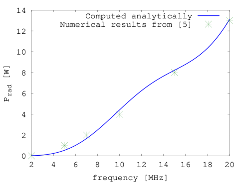
Figure 9: Comparison between the radiated power for a matched line from Table 1 of [5] with our results for a matched line in Eq. (13) for different frequencies.

TABLE II: The numerical data from Figure 9 and the relative error.

Frequency [MHz]	[5]	theoretical (Eq. 13)	% error
2	0	0.0165	-100
5	1	0.5359	87
7	2	1.664	20
10	4	4.411	-9.32
15	8	8.225	-2.73
20	13	13.11	-0.84

We see a good match for the high frequencies (big electric delay), and it deteriorates at small electric delays. But the result 0 for the frequency of 2 MHz is clearly incorrect, so we may understand that the accuracy of the results in [5] is low at small electric delays, for which the relative radiated power is small.

Another calculation in [5] is for a non matched TL, with end loads $R_{L}$=10, 50, 500$\,\Omega$, 1, 5, 10, and 50$~{}k\Omega$, all cases at frequency 10 MHz, carrying a net power of 1000 W. We compare those results with the results of Eq. (21). First $k=2\pi f/c=0.2094$ [1/m] is fixed, and we calculate for each load resistance $R_{L}$

$$|\Gamma|=\left|\frac{R_{L}-Z_{0}}{R_{L}+Z_{0}}\right|,$$ (38)

from which the forward power values for each case are given by

$$P^{+}=\frac{P}{1-|\Gamma|^{2}}=\frac{1000}{1-|\Gamma|^{2}}.$$ (39)

The forward current values for each case are given by $|I^{+}|=\sqrt{P^{+}/Z_{0}}$ and the backward current values for each case are given by $|I^{-}|=|\Gamma||I^{+}|$. Setting the values in Eq. (21), we compare the results of [5] for the unmatched line at 10MHz (Table 2 in [5]), with the results of Eq. (21) in Figure 10 and Table III.

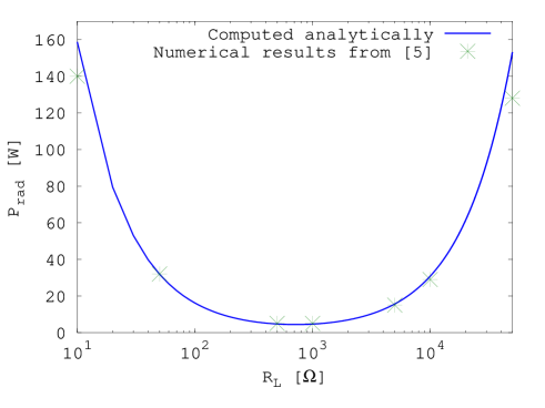
Figure 10: Comparison between the radiated power for a non matched line from Table 2 of [5] with our results for a non matched line in Eq. (21) for different load resistances.

TABLE III: The numerical data from Figure 10 and the relative error.

Load $R_{L}$ [$\Omega$]	[5]	theoretical (Eq. 21)	% error
10	140	158.83	-11.85
50	32	31.91	0.28
500	5	4.70	6.38
1k	5	4.65	7.53
5k	15	15.63	-4.03
10k	29	30.79	-5.81
50k	128	153.19	-16.44

The match between the results is good, except for the first and last cases, in which the radiated power is big and approaches the order of magnitude of the net power (1000 W). This may be due to the limitations of the current theory to small losses that almost do not affect the basic electromagnetic solution (see Introduction).

III-E Comparison with [6]

In 2006 Nakamura et. al. published the paper “Radiation Characteristics of a Transmission Line with a Side Plate” [6] which intends to reduce radiation losses from a twin lead TL using a side plate. The side plate is a perfect conductor put aside the transmission line, to create opposite image currents, and hence reduce the radiation.

The authors first derived the radiation from a TL without the side plate, obtaining an integral (Eq. 20 in [6]) which they computed numerically. The numerical integration result is shown in Figure 6 of [6], where the solid line represents the free space case.

We compare our analytic result in Eq. (13), with the numerical result shown in Figure 6 of [6]. First, $I_{0}$ in  [6] is a forward current, and from Eq. (19) in  [6], it is evident that they used RMS values. They used $I_{0}=1$A, hence we set $|I^{+}|=1$A in Eq. (13). $2h$ is the distance between the conductors in  [6], equivalent to $d$ in this work, and they used $h\lambda=0.1$, therefore $(kd)^{2}=(4\pi h/\lambda)^{2}=1.5791$ in Eq. (13), so that the total radiated power for the case displayed in Figure 6 of [6] is

$$P_{rad}= 60\times 1\times 1.5791\left[1-\operatorname{sinc}(4kL)\right]=$$

$$94.746[W]\left[1-\operatorname{sinc}\left(\frac{2L}{\lambda}4\pi\right)\right],$$ (40)

and we wrote the argument of the sinc function in terms of $2L/\lambda$, i.e. the TL length in wavelengths. This result is displayed in Figure 11, in which we show the radiated power as function of the TL length in wavelengths. The authors did not supply the numerical data to reproduce Figure 6 of [6], and we did not want to copy

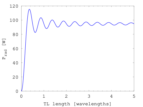
Figure 11: Recalculation of the solid line in Figure 6 of [6], using Eq. (13).

the figure into this work for comparison, but we checked very carefully that indeed our calculation shown in Figure 11 completely overlaps the solid line in Figure 6 of [6].

We compare as well the radiation patterns obtained in [6] with ours (Eq. 14) in Figure 12.

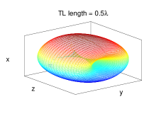
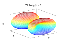
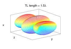
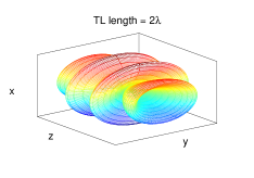
Figure 12: Radiation pattern $D^{+}$ calculated from Eq. (14) for the cases of TL lengths $n\lambda/2$, for n=1 to 4. They are identical to the parallel cases shown in Figure 5, panel(a) of [6]. Note that the definitions of the $x$ and $z$ axes are swapped in [6] compared to our definitions, we therefore showed them in an orientation which makes the comparison easy (i.e. our $z$ axis is oriented in the plots in the same direction as their $x$ axis). We remark that the pattern for the case $0.5\lambda$ is quite similar to this of a dipole antenna, because a short TL behaves similar to a small magnetic loop, i.e. a magnetic dipole.

We remark that $D^{+}(\theta)$ is not symmetric around $\theta=\pi/2$ in general (see Figure 4), but for the cases $kL=n\pi/2$ (integer $n$), i.e. the TL length is a multiple integer of half wavelength, displayed in Figure 12, $D^{+}(\theta)$ is symmetric around $\theta=\pi/2$, because $\sin^{2}(n\pi/2+x)=\sin^{2}(n\pi/2-x)$ for any $x$. The radiation patterns in Figure 12 are identical to the parallel cases shown in Figure 5, panel(a) of [6].

It is worthwhile to remark that the radiation pattern (Eq. 14) does not depend on the distance between the conductors $d$ (or $2h$ in [6]), hence the annotation of $h/\lambda=0.1$ in Figure 5 of [6] is redundant, and probably has been added to the caption because the authors computed the radiation patterns numerically for $h/\lambda=0.1$, without deriving an analytic expression.

III-F Comparison with [15, 16]

References [15, 16] analyze the radiation from a “U” shaped antenna (see Figure 13) and showed that its radiation pattern is uniform.

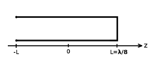
Figure 13: Transmission line of length $\lambda/4$, open at one termination, and shorted at the other, represents a “U” shaped antenna.

Using $\Gamma=-1$ (shorted termination) and $kL=\pi/4$ the radiation pattern in Eq. (23) is:

$$D=\sin^{2}\left[(\pi/2)\sin^{2}(\theta/2)\right]+\sin^{2}\left[(\pi/2)\cos^{2}(\theta/2)\right]=1.$$ (41)

Using $(\pi/2)\cos^{2}(\theta/2)=(\pi/2)-(\pi/2)\sin^{2}(\theta/2)$ one easily remarks that (41) is 1, describing uniform radiation, as mentioned in [15, 16]. This does not contradict the “hairy-ball” theorem [23], because this theorem states that any real tangential field must be 0 at least at one point on a sphere, and by real one means: having the same phase everywhere.

And indeed the separate fields associated with $I^{+}$ and $I^{-}$ (each one “real” in the above sense) given in Eqs. (9) and (17) are 0 at points $\theta=0$ and $\pi$ respectively. From Eq. (22), the relation between the forward and backward wave is $I^{-}=-jI^{+}$, and after summing the fields by setting this relation into Eq. (19), the far magnetic field is

$$\mathbf{H}=G(r)2kdI^{+}$$

$$[-\boldsymbol{\widehat{\varphi}}\cos\varphi e^{-j(\pi/2)\cos^{2}(\theta/2)}+\boldsymbol{\widehat{\theta}}\sin\varphi e^{j(\pi/2)\cos^{2}(\theta/2)}],$$ (42)

which has a constant amplitude everywhere, but a changing phase, which cannot be factored out to get a “real” field. This complex field manifests a linear polarization at $\theta=0$ and $\pi$, circular polarization at $\theta=\pi/2$ and $\varphi$ multiple of $\pi/4$, and elliptic elsewhere, compare with [15, 16].

IV Infinite and semi-infinite TL analysis

As we know, there are no infinite or semi-infinite TL in reality, but the literature considers those kind of TL as limiting cases, and as we shall see, the analysis of the infinite and semi-infinite TL supplies an additional insight and validation of the results obtained in the Section II, as shown in the following subsections.

Certainly those cases can be considered only in absence of other losses, like ohmic or dielectric, for which infinite TL have infinite losses. As one remarks, the radiation losses of finite TL reach an asymptotic value for long TL, so that one may expect that infinite or semi-infinite TL do not radiate an infinite power.

IV-A Infinite TL

For an infinite TL, carrying a forward wave, we set $z_{1}=-L$ and $z_{2}=L$ in the result (A.13) and considering $L\rightarrow\infty$ (i.e. for finite $z$ and $\rho$, $L\gg|z|,\rho$) we obtain

$$A_{z}=\frac{\mu_{0}I^{+}}{4\pi}d\cos\varphi\frac{2e^{-jkz}}{\rho}.$$ (43)

Certainly, we do not have in this case $x$ directed currents, so we obtain from Eq. (43):

$$\mathbf{H}=\frac{1}{\mu_{0}}\boldsymbol{\nabla}\times\mathbf{A}=\frac{e^{-jkz}}{2\pi}\frac{I^{+}d}{\rho^{2}}[-\widehat{\boldsymbol{\rho}}\sin\varphi+\widehat{\boldsymbol{\varphi}}\cos\varphi]$$ (44)

and

$$\mathbf{E}=\frac{1}{j\omega\epsilon_{0}}\boldsymbol{\nabla}\times\mathbf{H}=\eta_{0}\frac{e^{-jkz}}{2\pi}\frac{I^{+}d}{\rho^{2}}[\widehat{\boldsymbol{\rho}}\cos\varphi+\widehat{\boldsymbol{\varphi}}\sin\varphi],$$ (45)

which are the static $\mathbf{H}$ and $\mathbf{E}$ fields multiplied by the forward wave propagation factor $e^{-jkz}$.

We remark that in Appendix A we considered the far field ($k\rho\gg 1$), so the fields in Eqs. (44) and (45) are correct far from the TL, and their diverging at $\rho=0$ is an artifact of this far field approximation. But even in the far field, writing them in spherical coordinates so that $\rho=r\sin\theta$, the fields decay like $1/r^{2}$ and there is no “radiating” term decaying like $1/r$.

This is also evident from the Poynting vector:

$$\mathbf{S}=\mathbf{E}\times\mathbf{H}^{*}=\eta_{0}\frac{1}{4\pi^{2}}\frac{|I^{+}|^{2}d^{2}}{\rho^{4}}\widehat{\mathbf{z}},$$ (46)

which is only in the $z$ direction, representing the power carried by the TL.

Given the fact that the fields in Eqs. (44) and (45) decay much faster than radiating fields, hence are negligible relative to them far from the TL, it is convenient to define a typical distance $\rho_{0}$ from the TL, so that

$$\text{Static near field is dominant if}\,\,\rho<\rho_{0}$$

$$\text{Radiation field is dominant if}\,\,\rho>\rho_{0}.$$ (47)

There are no radiation fields in this subsection, but the relation (47) will be referred to in the next subsection, analyzing semi-infinite TL.

Another way of understanding $\rho_{0}$ is by integrating the Poynting vector to obtain the forward power $P^{+}$

$$P^{+}=\iint_{-\infty}^{\infty}dxdy\,\mathbf{S}\cdot\widehat{\mathbf{z}},$$ (48)

and here one has to use the exact fields in the expression for $\mathbf{S}$ (not the far fields in Eqs. (44) and (45)). To obtain $P^{+}$ with a “reasonable” required accuracy, one does not need to integrate to infinity, but rather

$$P^{+}\simeq\int_{0}^{2\pi}d\varphi\int_{0}^{\rho_{0}}d\rho\,\rho\,\mathbf{S}\cdot\widehat{\mathbf{z}},$$ (49)

so that $\rho_{0}$ is the radial distance from the TL (in cylindrical coordinates) within which the near fields are significant.

IV-B Semi-infinite TL

We analyze here a semi-infinite TL carrying a forward wave. The TL can be either from $z=-\infty$ to 0 (Figure 14) or from $z=0$ to $\infty$ (Figure 15). We note that in both cases we have to consider also the contribution of the $x$ directed current at the termination at $z=0$.

For the first case we set $z_{1}=-L$, $z_{2}=0$ in Eq. (A.13) and taking $L\rightarrow\infty$ we obtain

$$A_{z\,\,RT}=\frac{\mu_{0}I^{+}}{4\pi}d\cos\varphi\left[\frac{2e^{-jkz}}{\rho}-\frac{\rho}{r-z}\frac{e^{-jkr}}{r}\right]$$ (50)

and from Eq. (A.16) for $z_{2}=0$:

$$A_{x\,\,RT}=-\mu_{0}I^{+}d\frac{e^{-jkr}}{4\pi r},$$ (51)

while for the second case we set $z_{1}=0$, $z_{2}=L$ in Eq. (A.13) and taking $L\rightarrow\infty$ we obtain

$$A_{z\,\,LT}=\frac{\mu_{0}I^{+}}{4\pi}d\cos\varphi\left[\frac{\rho}{r-z}\frac{e^{-jkr}}{r}\right]$$ (52)

and from Eq. (A.16) for $z_{1}=0$:

$$A_{x\,\,LT}=\mu_{0}I^{+}d\frac{e^{-jkr}}{4\pi r},$$ (53)

where the subscripts RT and LT mean “right terminated” and “left terminated” TL, respectively.

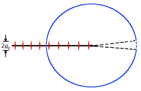
Figure 14: Semi-infinite TL from $z=-\infty$ to the center of coordinates at $z=0$. The blue circle represents the wave front of the outgoing spherical wave radiation in the second part of Eq. (50) and the red wave fronts represent the near plane wave field in the first part of Eq. (50). The near plane wave and spherical wave cancel each other in the paraxial region $z>0$ and $\rho<\rho_{0}$, see Eq. (54). The spherical wave is shown dashed blue in the canceling region, which occurs within a cone $\Delta\theta=\rho_{0}/r$ (dashed black line). The cone gets narrower as the distance from the center of coordinates $r$ increases.

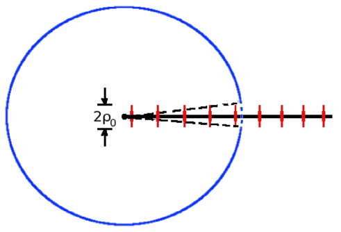
Figure 15: Semi-infinite TL from the center of coordinates at $z=0$ to $z=\infty$. The blue circle represents the wave front of the outgoing spherical wave radiation (Eq. (52)), but behaves in the paraxial region $z>0$ and $\rho<\rho_{0}$, like the near plane wave in the first part of Eq. (50), according to Eq. (54). Therefore, in this paraxial region the spherical wave front (dashed blue) does not represent radiation, but rather the near plane wave. Like in Figure 14, this paraxial region is within the cone $\Delta\theta=\rho_{0}/r$ (dashed black line), which gets narrower as the distance from the center of coordinates $r$ increases.

Looking at the RT configuration in Eq. (50), we see that it includes also the near field expression of the infinite TL from Eq. (43) for all $z$ in spite of the fact that the TL is in the region $z<0$ and terminates at $z=0$. This is explained by the fact that for $z>0$ and small $\rho$ (typically $\rho<\rho_{0}$, see (47)), $r\approx z+\frac{\rho^{2}}{2z}$, so that $r-z\approx\frac{\rho^{2}}{2z}$, resulting in

$$\left.\frac{\rho}{r-z}\frac{e^{-jkr}}{r}\right|_{\begin{subarray}{c}z>0\\ \rho<\rho_{0}\end{subarray}}\simeq\frac{2e^{-jkz}}{\rho},$$ (54)

which means that the spherical wave in the second part of Eq. (50) describes radiation everywhere except in a cone around $\theta=0$ where it is canceled by the near plane wave in the first part of Eq. (50), see Figure 14.

For the LT configuration the spherical wave in Eq. (52) represents radiation except inside a cone around $\theta=0$, where it equals the near plane wave in the first part of Eq. (50) (according to Eq. (54)), which does not have radiating fields, see Figure 15.

So to calculate the radiated power $P_{rad}^{+}$, one may either use the second part of Eq. (50) together with Eq. (51), or Eq. (52) together with Eq. (53), excluding the paraxial region around $\theta=0$. This exclusion is meaningless from the point of view of the calculation, because as the distance from the center of coordinates $r$ increases this region reduces to a singular point. The spherical potential vectors for the RT and LT configurations differ only by sign, so both yield the same result for $P_{rad}^{+}$. Using the RT configuration, we rewrite

$$A_{z}=\mu_{0}F_{(z)}(\theta,\varphi)G(r),$$ (55)

where

$$F_{(z)}(\theta,\varphi)=-I^{+}d\cos\varphi\frac{\sin\theta}{1-\cos\theta},$$ (56)

is the directivity function. We calculate now the radiating electric and magnetic fields, i.e. the part of the fields which decays like $1/r$, by approximating $\boldsymbol{\nabla}\simeq-jk\mathbf{\widehat{r}}$, obtaining

$$\mathbf{H}_{(z)}=jkF_{(z)}(\theta,\varphi)\sin\theta G(r)\boldsymbol{\widehat{\varphi}},$$ (57)

and $\mathbf{E}_{(z)}=\eta_{0}\mathbf{H}_{(z)}\times\mathbf{\widehat{r}}$. Now we rewrite (51):

$$A_{x}=\mu_{0}F_{(x)}(\theta,\varphi)G(r),$$ (58)

where the directivity function $F_{(x)}$ is

$$F_{(x)}(\theta,\varphi)=-I^{+}d,$$ (59)

The fields are $\mathbf{H}_{(x)}=(-jk\mathbf{\widehat{r}})\times(A_{x}\mathbf{\widehat{x}})/\mu_{0}$

$$\mathbf{H}_{(x)}=-jk(\cos\theta\cos\varphi\boldsymbol{\widehat{\varphi}}+\sin\varphi\boldsymbol{\widehat{\theta}})G(r)F_{(x)},$$ (60)

and $\mathbf{E}_{(x)}=\eta_{0}\mathbf{H}_{(x)}\times\mathbf{\widehat{r}}$. Adding up the fields $\mathbf{H}_{(z)}+\mathbf{H}_{(x)}$ we obtain

$$\mathbf{H}^{+}=-jkG(r)I^{+}d[\boldsymbol{\widehat{\varphi}}\cos\varphi-\boldsymbol{\widehat{\theta}}\sin\varphi].$$ (61)

We named it $\mathbf{H}^{+}$, because it is the radiating field of a forward wave. and

$$\mathbf{E}^{+}=\eta_{0}\mathbf{H}^{+}\times\mathbf{\widehat{r}}$$ (62)

resulting in Poynting vector $\mathbf{E}^{+}\times\mathbf{H}^{+*}$ :

$$\mathbf{S}^{+}=30\,\Omega\frac{(kd)^{2}\mathbf{\widehat{r}}}{4\pi r^{2}}|I^{+}|^{2},$$ (63)

So that the total radiated power for a forward wave is

$$P_{rad}^{+}=\int_{0}^{2\pi}\int_{0}^{\pi}\sin\theta d\theta d\varphi r^{2}\mathbf{\widehat{r}}\cdot\mathbf{S}=30\,\Omega|I^{+}|^{2}(kd)^{2}$$ (64)

It is clear from Eqs. (61) and (63) that this is an isotropic radiation. Calculating $D^{+}=4\pi r^{2}S_{r}^{+}/P_{rad}^{+}$, one obtains

$$D^{+}=1,$$ (65)

so that we encounter again an isotropic radiation, but contrary to the case shown in Section III-F, here the polarization is linear. This is possible because the radiation field is not the only field far from the origin, and the near plane wave is also present, see Figures 14 and 15.

It is worthwhile at this point to understand the connection between the radiation of a finite TL and a semi-infinite TL. In reality, a semi-infinite TL is a very long TL, for which we analyze the termination near to “our” side, while someone else analyzes the termination near to “his/her side”, as shown in Figure 16.

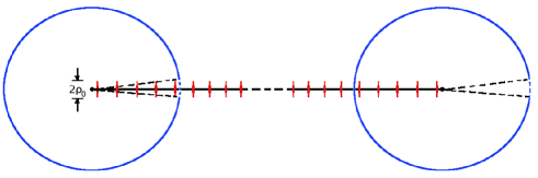
Figure 16: Very long TL, carrying a forward wave, for which one considers each termination as the termination of a semi-infinite TL. Each termination radiates the power $30\,\Omega|I^{+}|^{2}(kd)^{2}$, so that the whole TL radiates $60\,\Omega|I^{+}|^{2}(kd)^{2}$, the asymptotic value in Eq. (13).

Figure 17 shows schematically how the power radiated by a TL carrying a forward wave, gradually changes as the TL length increases.

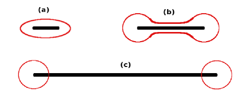
Figure 17: A schematic diagram showing the connection between the radiation of finite TL and semi-infinite TL carrying a forward wave. The red lines are hand drawn and go around the element considered for the calculation of the radiation, so their shape is meaningless. Panel (a) shows a short TL radiating the power $60\,\Omega(kd)^{2}|I^{+}|^{2}\left[1-\operatorname{sinc}(4kL)\right]$ according to Eq. (13). Panel (b) shows a TL longer than several wavelengths, for which $|\operatorname{sinc}(4kL)|\ll 1$, which practically radiates $60\,\Omega(kd)^{2}|I^{+}|^{2}$, but still considered a single radiating element. Panel (c) shows a very long TL, like in Figure 16, which is analyzed as two separate radiating elements (as shown in Figures 14 and 15), each one radiating $30\,\Omega(kd)^{2}|I^{+}|^{2}$, according to Eq. (64), in total the same as in panel (b).

Till here we considered only a forward wave, and that is what one usually considers for a semi-infinite TL from $z=0$ to $\infty$ (LT case), but for the RT case terminated by a non matched load, one can have both forward and backward waves. The generalization for this case is done like in Section II-B, and the total radiated power in presence of a forward and backward wave is

$$P_{rad}=30\,\Omega(kd)^{2}(|I^{+}|^{2}+|I^{-}|^{2}),$$ (66)

so that the interference between the waves does not contribute to the radiated power, similarly to the case of a finite TL.

V Radiation resistance

The radiation resistance has already been worked out in Section III-C, for comparison with [4]. It is defined by $r_{\text{rad}}=P_{\text{rad}}/|I|^{2}$, $P_{\text{rad}}$ being the total power radiated by the TL, and $I$ the current at the generator side (in Figure 5 it is $I(-L)$). The radiation resistance is given in Eq. (36) and is identical to Eq. (5) in [4].

However, we remark that $r_{\text{rad}}$ in Eq. (36) goes to infinity if $|\Gamma|=1$ and $4kL-\angle\Gamma=2\pi n$ ($n$ integer). For example if $Z_{L}$ in Figure 5 is $\infty$ (open TL), $\Gamma=1$, so that $I(L)=0$. If the length of the TL $2L$ is a multiple integer of $\lambda/2$, also the current at the generator side $I(-L)=0$. This is shown schematically in Figure 18, for $n=1$.

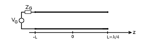
Figure 18: Open ended transmission line, of length $2L=\lambda/2$. The current is 0 at both TL ends. The radiation resistance in Eq. (36) (or Eq. (5) in [4]) fails in this case, resulting infinity.

This case represents resonance (infinite VSWR) and current at generator side 0. This of course does not mean that the generator does not have to compensate for the radiated power, but rather a fail of the small radiation losses approximation. In such case $P^{+}=|I^{+}|^{2}Z_{0}$ equals $P^{-}=|I^{-}|^{2}Z_{0}$ so that the net power carried by the TL $P=P^{+}-P^{-}=0$, hence the radiated power $P_{rad}$ is infinitely bigger than the net power $P$ transferred by the TL.

We derive here a more robust radiation resistance, valid for any TL configuration. We still assume $P^{+}_{rad}\ll P^{+}$ (small relative losses), but the total radiated power $P_{rad}$ is allowed to be bigger than the net power $P$. Given the fact that the interference between the forward and backward waves does not contribute to the radiated power (see (Eq. 21)), we may consider the separate loss of the forward or backward wave.

The relation $P_{rad}^{+}/P^{+}$ in Eq. (15), equal also to $P_{rad}^{-}/P^{-}$, is written as if $P^{+}$ would be a constant, but $P^{+}$ is only approximately constant for $P^{+}_{rad}\ll P^{+}$. Looking at the configuration in Figure 5, by conservation of energy, the power radiated by a forward wave $P^{+}_{rad}$ must be the difference $P^{+}(-L)-P^{+}(L)$, which is small relative to the individual values of $P^{+}(-L)$ and $P^{+}(L)$. We may therefore express $P^{+}(L)=P^{+}(-L)-P^{+}_{rad}$, but considering $P^{+}_{rad}\ll P^{+}$, this may be written as $P^{+}(L)=P^{+}(-L)\left[1-P^{+}_{rad}/P^{+}\right]$, or more conveniently $P^{+}(L)=P^{+}(-L)\exp(-P^{+}_{rad}/P^{+})$.

The small decay factor $P^{+}_{rad}/P^{+}$ (or $P^{-}_{rad}/P^{-}$ for the backward wave) is minus twice the imaginary part of the TL electrical length $2\text{Im}\{\Theta\}$ according to Eq. (30), so we may describe the dynamics of $P^{+}$ or $P^{-}$ along the TL

$$P^{+}(L)=P^{+}(-L)e^{2\text{Im}\{\Theta\}}$$ (67)

$$P^{-}(-L)=P^{-}(L)e^{2\text{Im}\{\Theta\}}$$ (68)

where Im$\{\Theta\}<0$ always. Given $P^{\pm}$ are proportional to $|I^{\pm}|^{2}$ respectively, the forward and backward currents decay according to $\text{Im}\{\Theta\}$, in addition to their accumulated phase, so we express

$$I^{+}(L)=I^{+}(-L)e^{-j2kL}e^{\text{Im}\{\Theta\}},$$ (69)

$$I^{-}(-L)=I^{-}(L)e^{-j2kL}e^{\text{Im}\{\Theta\}},$$ (70)

At the load side $I^{-}(L)=-\Gamma I^{+}(L)$, so using Eqs. (69) and (70), we express the total current near the generator $I(-L)=I^{+}(-L)+I^{-}(-L)$:

$$I(-L)=I^{+}(-L)\left[1-\Gamma e^{-j4kL}e^{2\text{Im}\{\Theta\}}\right]$$ (71)

which for $|\text{Im}\{\Theta\}|\ll 1$ can be written:

$$I(-L)=I^{+}(-L)\left[1-\Gamma e^{-j4kL}(1+2\text{Im}\{\Theta\})\right]$$ (72)

Using Eqs. (35), (21) and the relation $-2\text{Im}\{\Theta\}=P^{+}_{rad}/P^{+}$ from Eq. (15) we obtain a more accurate, explicit expression for the radiation resistance

$$r_{\text{rad}}=\frac{60\,\Omega(kd)^{2}\left[1-\operatorname{sinc}(4kL)\right](1+|\Gamma|^{2})}{|1-\Gamma e^{-4jkL}\{1-(60\,\Omega/Z_{0})(kd)^{2}\left[1-\operatorname{sinc}(4kL)\right]\}|^{2}}.$$ (73)

If $\Gamma e^{-4jkL}$ is far from 1, the last term in the denominator is negligible, and one recovers the approximate Eq. (36). On the other hand if $\Gamma e^{-4jkL}=1$ (resonance), one obtains

$$r_{\text{rad}}=\frac{2Z_{0}^{2}}{60\,\Omega(kd)^{2}\left[1-\operatorname{sinc}(4kL)\right]}.$$ (74)

which is big, because $kd\ll 1$, but not infinite. For the special case described in Figure 18, $\Gamma=1$ and $4kL=2\pi$, the $\operatorname{sinc}$ function is 0, so that $r_{\text{rad}}$ reduces to $2Z_{0}^{2}/[60\,\Omega\,(kd)^{2}]$.

VI Conclusions

We derived in this work a general radiation losses model for two-conductors transmission lines (TL) in free space. We considered any combination of forward and backward waves (i.e. any termination), and also any TL length, analyzing infinite, semi-infinite and finite TL.

One important finding is that the interference between forward and backward waves does not contribute to the radiated power (Eq. (21)), which has been also validated by the comparisons with [3, 4, 5, 15, 16], in the sense that those comparisons would have failed if Eq. (21) were incorrect.

This property allowed us to consider the separate losses for the forward an backward wave for the calculation of the radiation resistance in Section V. This radiation resistance reduces correctly far from resonance to this calculated in [4] (Eq. 36), but handles correctly the resonant case.

Another novelty of this work is the analysis of the semi-infinite TL which clearly shows that the radiation from TL is mainly a termination effect. We found an isotropic radiation from the semi-infinite TL, which is possible due to the fact that the radiation fields are not the only far fields, as shown in Figures 14 and 15. The semi-infinite TL radiation results are consistent with finite TL results, so that a very long TL can be regarded as two semi-infinite TLs, as shown in Figure 17.

Although previous works [4, 3, 5, 6, 7] considered exclusively the twin lead cross section, the formalism developed in this work is valid for any cross section. We showed this in Section III-A by successfully comparing the analytic results with simulation of ANSYS-HFSS commercial software for a parallel cylinders cross section (Figure 6), in which the radius was not small relative to the distance between the centers of the cylinders. Appendix B explains how to calculate the parameters needed to derive the radiation for any TL cross section.

Some comments on the generalization of this research for TL in dielectric insulator. The case of TL in dielectric insulator is solvable analytically, but much more involved than the free space case. The fact that the TL propagation wavenumber $\beta$ is different form the free space wavenumber $k$ by itself complicates the mathematics, but in addition it comes out that one needs to consider in this case also polarization currents, which further complicate the results. Radiation from TL in dielectric insulator will be published separately, as Part II of this study.

Appendix A Far vector potential of separated two-conductors transmission line

We show in this appendix that for the purpose of calculating the far fields from a two ideal conductor transmission line (TL) in free space, having a well defined separation between the conductors, as shown in Figure 1, one can use an equivalent twin lead, provided the separation is much smaller than the wavelength.

For simplicity we use a forward wave (propagating like $e^{-jkz}$), but the same conclusion is valid for a combination of waves. In the far field the $z$ directed magnetic potential vector $A_{z}$ is expressed as

$$A_{z}=\mu_{0}\int_{z_{1}}^{z_{2}}dz^{\prime}\oint dc\,K_{z}(c)e^{-jkz^{\prime}}G(R)$$ (A.1)

where the $dz^{\prime}$ integral goes on the whole length of the TL,

$$G(s)=\frac{e^{-jks}}{4\pi s}$$ (A.2)

is the 3D Green’s function, $K_{z}$ is the surface current distribution as function of the contour parameter $c$ (i.e. $c_{1}$ and $c_{2}$, see Figure 1) which is known from electrostatic considerations, and $R$ is the distance from the integration point on the contour of the conductors to the observer:

$$R=\sqrt{(x-x^{\prime}(c))^{2}+(y-y^{\prime}(c))^{2}+(z-z^{\prime})^{2}}.$$ (A.3)

Changing variable $z^{\prime\prime}=z^{\prime}-z$ in Eq. (A.1), one obtains

$$A_{z}=\mu_{0}e^{-jkz}\int_{z_{1}-z}^{z_{2}-z}dz^{\prime\prime}\oint dc\,K_{z}(c)e^{-jkz^{\prime\prime}}G(R),$$ (A.4)

redefining $R=\sqrt{(x-x^{\prime}(c))^{2}+(y-y^{\prime}(c))^{2}+(z^{\prime\prime})^{2}}$. For a far observer, at distance $\rho\equiv\sqrt{x^{2}+y^{2}}$ from the TL, so that $\rho$ is much bigger than the transverse dimensions of the TL one approximates $R$ in cylindrical coordinates as

$$R\simeq r-\frac{\rho}{r}\left[x^{\prime}(c)\cos\varphi+y^{\prime}(c)\sin\varphi\right],$$ (A.5)

where $r(z^{\prime\prime})\equiv\sqrt{(z^{\prime\prime})^{2}+\rho^{2}}$. We keep for now everything in cylindrical coordinates, to be able to handle infinite or semi-infinite lines. Using this in Eq. (A.4), one obtains

$$A_{z}= \mu_{0}e^{-jkz}\int_{z_{1}-z}^{z_{2}-z}dz^{\prime\prime}\frac{e^{-jk[z^{\prime\prime}+r(z^{\prime\prime})]}}{4\pi r(z^{\prime\prime})}$$

$$\oint dc\,K_{z}(c)e^{jk(\rho/r)[x^{\prime}(c)\cos\varphi+y^{\prime}(c)\sin\varphi]}.$$ (A.6)

We consider the higher modes to be in deep cutoff, so that $kx^{\prime}(c),ky^{\prime}(c)\ll 1$, hence

$$A_{z}\approx \mu_{0}e^{-jkz}\int_{z_{1}-z}^{z_{2}-z}dz^{\prime\prime}\frac{e^{-jk[z^{\prime\prime}+r(z^{\prime\prime})]}}{4\pi r(z^{\prime\prime})}\oint dc\,K_{z}(c)$$

$$\left\{1+jk(\rho/r)[x^{\prime}(c)\cos\varphi+y^{\prime}(c)\sin\varphi]\right\}.$$ (A.7)

Separating the contour integral $\oint dc=\oint dc_{1}+\oint dc_{2}$, where $c_{1,2}$ are the contours of the “upper” and “lower” conductors respectively (see Figure 1), and using

$$\oint dc_{1}K_{z}(c_{1})=-\oint dc_{2}K_{z}(c_{2})=I^{+}$$ (A.8)

so that the integral on each surface current distribution results in the total current, which we call $I^{+}$, because it represents a forward wave. Given that for a two-conductors TL there is only one (differential) TEM mode, this current is equal, but with opposite signs on the conductors. We may define the 2D vector $\boldsymbol{\rho}(c)\equiv(x^{\prime}(c),y^{\prime}(c))$, from which one defines the vector distance between the center of the surface current distributions

$$\mathbf{d}\equiv\left[\oint dc_{1}K_{z}(c_{1})\boldsymbol{\rho}(c_{1})+\oint dc_{2}K_{z}(c_{2})\boldsymbol{\rho}(c_{2})\right]/I^{+}.$$ (A.9)

From this point, the original cross section is relevant only for calculating the equivalent separation vector $\mathbf{d}$ in the twin lead representation, and the remaining calculation bases solely on this twin lead representation. In appendix B we show examples for the calculation of the twin lead equivalent for given cross sections.

Using the twin lead representation, Eq. (A.7) may be rewritten

$$A_{z}= \mu_{0}e^{-jkz}I^{+}jk[d_{x}\cos\varphi+d_{y}\sin\varphi]$$

$$\int_{z_{1}-z}^{z_{2}-z}dz^{\prime\prime}\frac{e^{-jk[z^{\prime\prime}+r(z^{\prime\prime})]}}{4\pi r(z^{\prime\prime})}\frac{\rho}{r(z^{\prime\prime})},$$ (A.10)

where $d_{x}$ and the $d_{y}$ are the $x$ and $y$ components of the vector $\mathbf{d}$. This represents a twin lead, as shown in Figure 2, and is actually a 2D dipole approximation of the TL. Without loss of generality, one redefines the $x$ axis to be aligned with $\mathbf{d}$, so that $d_{x}=d$ and $d_{y}=0$, obtaining

$$A_{z}=\mu_{0}e^{-jkz}I^{+}jkd\cos\varphi\int_{z_{1}-z}^{z_{2}-z}dz^{\prime\prime}\frac{e^{-jk[z^{\prime\prime}+r(z^{\prime\prime})]}}{4\pi r}\frac{\rho}{r(z^{\prime\prime})},$$ (A.11)

which is equivalent of having a current $I^{+}e^{-jkz}$ confined on the conductor at $x=d/2$ and the same current confined on the conductor $x=-d/2$ but defined in the opposite direction, representing a twin lead (see Figure 2). We are interested in radiation, so we require the observer to be many wavelengths far from the TL: $k\rho\gg 1$ and $kr\gg 1$, so that Eq. (A.11) may be further simplified to

$$A_{z}=-\frac{\mu_{0}I^{+}e^{-jkz}d\cos\varphi}{4\pi}\frac{\partial}{\partial\rho}\int_{z_{1}-z}^{z_{2}-z}dz^{\prime\prime}\frac{e^{-jk[z^{\prime\prime}+r(z^{\prime\prime})]}}{r(z^{\prime\prime})}.$$ (A.12)

The $dz^{\prime\prime}$ integral results in the exponential integral function $\operatorname{Ei}$ as follows

$$A_{z}= -\frac{\mu_{0}I^{+}e^{-jkz}d\cos\varphi}{4\pi}$$

$$\left.\frac{\partial}{\partial\rho}\operatorname{Ei}\left(-jk\left[z^{\prime\prime}+\sqrt{(z^{\prime\prime})^{2}+\rho^{2}}\right]\right)\right|_{z_{1}-z}^{z_{2}-z},$$ (A.13)

where the $\operatorname{Ei}$ function satisfies $d\operatorname{Ei}(s)/ds=e^{s}/s$.

The twin lead geometry also allows us to use simple models for the termination currents in the $x$ direction (see Figure 2), defining the $x$ component of the magnetic vector potential, calculated as:

$$A_{x\,1,2}=\pm\mu_{0}I^{+}\int_{-d/2}^{d/2}dx^{\prime}e^{-jkz_{1,2}}G(R_{1,2})$$ (A.14)

where the indices 1,2 denote the contributions from the termination currents at $z_{1,2}$, respectively, see (see Figure 2) and the distances $R_{1,2}$ of the far observer from the terminations may be expressed in spherical coordinates, as follows:

$$R_{1,2}\simeq r-z_{1,2}\cos\theta-x^{\prime}\sin\theta\cos\varphi,$$ (A.15)

The integral (A.14) is carried out for $kd\ll 1$, resulting in

$$A_{x\,1,2}=\pm\mu_{0}I^{+}dG(r)e^{-jkz_{1,2}(1-\cos\theta)}$$ (A.16)

Appendix B Computation of radiation parameters

To calculate the power radiated from a TL, of any cross section, one needs the separation vector $\mathbf{d}$, defined in Figure 1, calculated from Eq. (A.9). If one needs the normalized radiation due to a forward wave, one also needs to know the characteristic impedance $Z_{0}$. Those are obtained with the aid of the ANSYS 2D “Maxwell” simulation, from an electrostatic analysis. We ran the 2D “Maxwell” simulation on two cross sections shown in Figure B.1.

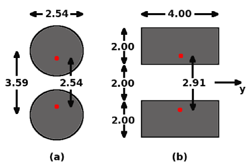
Figure B.1: Panel (a) shows a cross section of circular shaped conductors and panel (b) shows a cross section of rectangular shaped conductors. The sizes are in units of cm. The $y$ axis is horizontal, and the $x$ axis for each cross section is the symmetry axis. The red points show the current images which define the twin lead representation, and are referred further on.

It is to be mentioned that we know the analytic solution for the cross section in panel (a) from image theory [10], so that it can be used as a test for the quality of the numerical simulation. The magnitude of the electric fields measured for those cross sections is shown in Figure B.2.

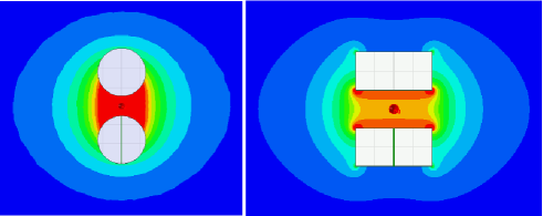
Figure B.2: The magnitude of the electric field, the hottest color representing high field and coldest color low (close to 0) field, for the circular shaped conductors cross section in the left panel and for the rectangular shaped conductors in the right panel. The red scars in the middle of the plots show the coordinate’s origin.

We remark that the surface currents, which are proportional to the (tangential) magnetic field on the conductors are also proportional to the (normal) electric field on the conductors. Given the surface currents $K_{z}(c_{1})>0$ and $K_{z}(c_{2})<0$ in Eq. (A.9), and using the field intensity which is positive, $E(c_{1})$ is proportional to $K_{z}(c_{1})$ and $E(c_{2})$ is proportional to $-K_{z}(c_{2})$, we may calculate the separation vector $\mathbf{d}$, using Eqs. (A.8) and (A.9), after replacing $K_{z}(c_{1})$ by $E(c_{1})$ and $K_{z}(c_{2})$ by $-E(c_{2})$ as follows

$$\mathbf{d}=\frac{\oint dc_{1}E(c_{1})\boldsymbol{\rho}(c_{1})-\oint dc_{2}E(c_{2})\boldsymbol{\rho}(c_{2})}{\oint dc_{1}E(c_{1})}.$$ (B.1)

For the cross sections in Figure B.1, the “positive” and “negative” conductors are symmetric, so that a given location vector $\boldsymbol{\rho}(c_{2})$ on the negative conductor, is the minus of the corresponding location vector $\boldsymbol{\rho}(c_{1})$ on the positive conductor, and by symmetry the magnitudes of the electric fields $E(c_{1})=E(c_{2})$, so that we may drop the second integral in the numerator of Eq. (B.1), and multiply the result by 2. Also by symmetry the $y$ component of $\mathbf{d}$ comes out 0, so that $d=|\mathbf{d}|=d_{x}$ represents the distance between the “image” currents in the twin lead model, and we obtained $d=2.54$ cm for the circular cross section (compares well with Eq. (25)), and $d=2.91$ cm for the rectangular cross section, as shown in Figure B.1.

We obtained from the 2D “Maxwell” simulation also the per unit length capacitances, which came out 31.5 pF/m and 33.51 pF/m for the circular and rectangular cross sections, respectively. The characteristic impedance $Z_{0}$ is calculated by $1/(Cc)$, where $c$ is the velocity of light in vacuum and $C$ is the per unit length capacitance, and come out 105.8$\,\Omega$ (compares well with Eq. (26)) and 99.51$\,\Omega$ for the circular and rectangular cross sections, respectively.

The procedure described in this section can be done for any cross section, and it supplies all the values needed to calculate the normalized radiation in Eq. (15). Its accuracy can be found by comparing the values obtained for $d$ and $Z_{0}$ for the circular cross section, with the theoretical values obtained from image theory and they fit with an inaccuracy of less than 0.5%.

Reuven Ianconescu graduated B.Sc (Summa cum laude) in 1987 and PhD in 1994, both in Electrical engineering at Tel Aviv university. He worked many years in R&D in the hi-tech industry, did a post-doc in the Weizmann Institute of Science, and is currently an academic staff member in Shenkar college of engineering and design. His research interests are: guided EM propagation, radiation and dynamics of charges and electrohydrodynamics.

Vladimir Vulfin has over 13 years of research experience in the areas of electromagnetic engineering. Since 2004 he worked in different companies as Electromagnetics Engineer. His job duties included design, simulations, implementations and measurements of antennas and microwave devices. Parallel to this, Vladimir was active as an external lecturer and instructor in different universities and colleges in Israel. He lead more than 100 degree final projects for students in Electrical Engineering Departments. Vladimir received the B.Sc and M.Sc. degrees in Electrical Engineering. Currently he is working towards his Ph.D degree at Ben Gurion University in the area of antennas and metamaterials.

References

- [1] R. Ianconescu and V. Vulfin, “TEM Transmission line radiation losses analysis”, Proceedings of the 46th European Microwave Conference, EuMW 2016, London, October 3-7
- [2] R. Ianconescu and V. Vulfin, “Simulation and theory of TEM transmission lines radiation losses”, ICSEE International Conference on the Science of Electrical Engineering, Eilat, Israel, November 16-18, 2016
- [3] C. Manneback, “Radiation from Transmission Lines”, Transactions of the American Institute of Electrical Engineers, Vol. XLII, pp. 289-301, 1923 ; C. Manneback, “Radiation from Transmission Lines”, Journal of the American Institute of Electrical Engineers, 42(2), pp. 95-105, 1923
- [4] J. E. Storer and R. King, Radiation Resistance of a Two-Wire Line, in Proceedings of the IRE, vol. 39, no. 11, pp. 1408-1412, doi: 10.1109/JRPROC.1951.273603, (1951)
- [5] G. Bingeman, “Transmission lines as antennas”, RF Design 2(1), pp. 74-82, 2001
- [6] T. Nakamura, N. Takase and R, Sato, “Radiation Characteristics of a Transmission Line with a Side Plate”, Electronics and Communications in Japan, Part 1, Vol. 89, No. 6, 2006
- [7] JR. Carson, Radiation from transmission lines, Journal of the American Institute of Electrical Engineers 40(10), pp. 789-90 (1921)
- [8] Midlands State University, Zimbabwe, educational document: http://www.msu.ac.zw/elearning/material/1343053427HTEL104
- [9] Collin, Robert E. Antennas and radiowave propagation, McGraw-Hill, 1985.
- [10] Orfanidis S.J., Electromagnetic Waves and Antennas, ISBN: 0130938556, (Rutgers University, 2002)
- [11] S. Ramo, J. R. Whinnery and T. Van Duzer, Fields and Waves in Communication Electronics, 3rd edition, Wiley 1994
- [12] E. C. Jordan and K. G. Balmain, Electromagnetic Waves and Radiating Systems, 2nd edition, Prentice Hall 1968
- [13] C. A. Balanis, Antenna Theory: Analysis and Design, 3rd edition, John Wiley & Sons, 2005
- [14] D. M. Pozar, Microwave Engineering, Wiley India Pvt., 2009
- [15] H. Matzner and K. T. McDonald, “Isotropic Radiators”, arXiv:physics/0312023
- [16] R. Guertler, ”Isotropic transmission-line antenna and its toroid-pattern modification.” IEEE Transactions on Antennas and Propagation 25(3), pp 386-392 (1977)
- [17] A. Gover, R. Ianconescu, C. Emma, P. Musumeci and A. Friedman, “Conceptual Theory of Spontaneous and Taper-Enhanced Superradiance and Stimulated Superradiance”, FEL 2015 Conference, August 23-28, Daejeon, Korea
- [18] R. Ianconescu, E. Hemsing, A. Marinelli, A. Nause and A. Gover, “Sub-Radiance and Enhanced-Radiance of undulator radiation from a correlated electron beam”, FEL 2015 Conference, August 23-28, Daejeon, Korea
- [19] A. Gover, R. Ianconescu, A. Friedman, C. Emma and P. Musumeci, “Coherent emission from a bunched electron beam: superradiance and stimulated-superradiance in a uniform and tapered wiggler FEL”, Nucl. Instr. Meth. Phys. Res. A, http://dx.doi.org/10.1016/j.nima.2016.12.038 , 2016
- [20] V. Vulfin and R. Ianconescu, Transmission of the maximum number of signals through a Multi-Conductor transmission line without crosstalk or return loss: theory and simulation, IET MICROW ANTENNA P, 9(13), pp. 1444-1452 (2015)
- [21] R. Ianconescu and V. Vulfin, Analysis of lossy multiconductor transmission lines and application of a crosstalk canceling algorithm, IET MICROW ANTENNA P, 11(3), pp. 394-401 (2016)
- [22] R. Ianconescu and V. Vulfin, “Simulation for a Crosstalk Avoiding Algorithm in Multi-Conductor Communication”, 2014 IEEE 28-th Convention of Electrical and Electronics Engineers in Israel, Eilat, December 3-5
- [23] Brouwer L.E. “On continuous vector distributions on surfaces.(2nd communication.)”, Koninklijke Nederlandse Akademie van Wetenschappen Proceedings Series B Physical Sciences. 12, pp 716-34 (1909)