Cracking of Charged Polytropes with Generalized Polytropic Equation of State

Abstract

We discuss the occurrence of cracking in charged anisotropic polytropes with generalized polytropic equation of state through two different assumptions; (i) by carrying out local density perturbations under conformally flat condition (ii) by perturbing anisotropy, polytropic index and charge parameters. For this purpose, we consider two different definitions of polytropes exist in literature. We conclude that under local density perturbations scheme cracking does not appears in both types of polytropes and stable configuration are observed, while with second kind of perturbation cracking appears in both types of polytropes under certain conditions.

Keywords: Self-gravitating objects; Cracking; Perturbations; Electromagnetic field .
PACS: 04.20.-q; 04.40.Dg; 04.50.Gh.

1 Introduction

The theory of polytropes is vital in the evolution of mathematical models of compact objects and it attracts many researchers due to its simple form. In the study of polytropes, the main attraction is Lane-Emden equation, which led us towards the illustration of various astrophysical phenomena. Chandrasekhar [1] initially developed the theory of polytropes in Newtonian frame work with the help of laws of thermodynamics. Topper [2, 3] used the hypothesis of quasi-static equilibrium form for the development of initial frame work of Newtonian polytropes. Kovetz [4] refined the work of Chandrasekhar [1] and reshaped the theory of polytropes. Abramowicz [5] was the first who presented higher dimension polytropes by developing Lane-Emden equation in higher dimension.

The study of electromagnetism and its effect on physical properties of astrophysical objects always fascinated the researches. Bekenstein [6] developed hydrostatic equilibrium equation (HEe) for the description of collapse of charged stars. Bonnor [7, 8] presented the study on charged compact objects and described how electromagnetism affects the gravitational collapse. Bondi [9] used isotropic coordinates to analyzed the contraction of stars in the presence of charged. Ray et al. [10] examined the properties of stars with higher densities and concluded that approximately $10^{20}$ coulomb charge can be hold by such stars. Herrera et al. [11] utilized structure scalars to illustrate compact objects having charged dissipative inner fluid distribution. Takisa and Maharaj [12] presented the mathematical model of charged compact objects with polytropic EoS.

The impact of anisotropy in the theory of general relativity is very important as we cannot study many physical phenomena without taking it into account. Cosenza et al. [13] presented a heuristic way for mathematical modeling of compact objects with anisotropic inner fluid distribution. Herrera and Santos [14] derived the anisotropic compact models in the frame work of general relativity. Herrera and Barreto [15] adopted a novel approach of effective variables for the description of physical variables involved in the anisotropic polytropic models. Herrera et al. [16] developed the governing equations in the presence of anisotropic stress for spherically symmetries. Herrera and Barreto [17, 18] used the concept of Tolman-mass to check the viability of anisotropic polytropic models. Herrera et al. [19] adopted conformally flat approach to reduced physical parameters for simplification of Lane-Emden equations of polytropes.

The stability analysis of any developed model of stars plays a key role in general relativity. Any developed model cannot be used for the description of stars unless it is critically analyzed for stability. Bondi [20] developed HEe for stability analysis of neutral stars. Herrera et al. [21] proposed a novel way for the analysis of spherical symmetric models by means of cracking (overturning), which described the behavior of fluid distribution just after equilibrium state has been perturbed through density perturbation. Gonzalez et al. [22, 23] provided an extension of Herrera et al. [21] by introducing local density perturbation (LDP). Azam et al. [24]-[28] used LDP for the analysis of various mathematical models of compact objects. Sharif and Sadiq [29] developed the model of charged polytropes. Azam et al. [30, 31] developed the general frame work for charged polytropes with generalized polytropic equation of state (GPEoS) for spherical and cylindrical symmetries. They analyzed these models by means of Tolman-mass and Whittaker mass for spherical and cylindrical symmetries, respectively. Herrera et al. [32] have discussed the effect of small fluctuations of local anisotropy of pressure, and energy density on spherical polytropes. Sharif and Sadiq [33] have examined the effects of charge on spherical polytropes. Azam and Mardan [34] refined the work [33] for the analysis of charged polytropes.

The plan of work is as follows. In section 2, we provide some basic equations. Section 3 and 4 are devoted for the analysis of cracking through LDP and parametric perturbation respectively. In the last section we conclude over results.

2 Einstein-Maxwell Field Equations

We consider static spherically symmetric space time

$$ds^{2}=-e^{\nu}dt^{2}+e^{\lambda}dr^{2}+r^{2}d\theta^{2}+r^{2}\sin^{2}\theta{d\phi^{2}},$$ (1)

where $\nu(r)$ and $\lambda(r)$ both depends only on radial coordinate $r$. The generalized form of energy-momentum tensor for charged anisotropic inner fluid distribution is given by

$$T_{ij}=(P_{t}+\rho)V_{i}V_{j}+g_{ij}P_{t}+(P_{r}-P_{t})S_{i}S_{j}+\frac{1}{4\pi}(F_{i}^{m}F_{jm}-\frac{1}{4}F^{mn}F_{mn}g_{ij}),$$ (2)

where $P_{t}$, $P_{r}$, $\rho$, $V_{i}$, $S_{i}$ and $F_{mn}$ represent the tangential pressure, radial pressure, energy density, four velocity, four vector and Maxwell field tensor for the inner fluid distribution. The Einstein-Maxwell field equations for line element Eq.$(\ref{1})$ are given by

$$\frac{\lambda^{\prime}e^{-\lambda}}{r}+\frac{(1-e^{-\lambda})}{r^{2}}=8\pi\rho+\frac{q^{2}}{r^{4}},$$ (3)

$$\frac{\nu^{\prime}e^{-\lambda}}{r}-\frac{(1-e^{-\lambda})}{r^{2}}=8\pi P_{r}-\frac{q^{2}}{r^{4}},$$ (4)

$$e^{-\lambda}\bigg{[}\frac{\nu^{\prime\prime}}{2}-\frac{\nu^{\prime}\lambda^{\prime}}{4}+\frac{\nu^{\prime^{2}}}{4}+\frac{\lambda^{\prime}-\nu^{\prime}}{2r}\bigg{]}=8\pi P_{t}+\frac{q^{2}}{r^{4}}.$$ (5)

Solving Eqs. $(\ref{7})$-$(\ref{9})$ simultaneously lead to HEe

$$\frac{dP_{r}}{dr}-\frac{2}{r}\Big{(}\Delta+\frac{qq^{\prime}}{8\pi r^{3}}\Big{)}+\Big{(}\frac{4\pi r^{4}P_{r}-q^{2}+mr}{r(r^{2}-2mr+q^{2})}\Big{)}(\rho+P_{r})=0,$$ (6)

where we have used $\Delta=(P_{t}-P_{r})$. We take the Reissner-Nordsträm space-time as the exterior geometry

$$ds^{2}=\Big{(}1-\frac{2M}{r}+\frac{Q^{2}}{r^{2}}\Big{)}dt^{2}-\Big{(}1-\frac{2M}{r}+\frac{Q^{2}}{r^{2}}\Big{)}^{-1}dr^{2}-r^{2}d\theta^{2}-r^{2}\sin^{2}\theta{d\phi^{2}}.$$ (7)

The junction conditions are very important in mathematical modeling of compact stars. They provide us the criterion for the collaboration of two metrics, which can results a physically viable solution [34, 35]. For smooth matching of two space times, we must have

$$e^{\nu}=e^{-\lambda}=\Big{(}1-\frac{2M}{r}+\frac{Q^{2}}{r^{2}}\Big{)},~{}~{}m(r)=M,~{}q(r)=Q,~{}P_{r}=0,$$ (8)

and Misner-Sharp mass [36] leads to

$$m(r)=\frac{r}{2}(1-e^{-\lambda}+\frac{q^{2}}{r^{2}}),$$ (9)

which has been used in the development of Lane-Emden equations [30].

3 Effect of Local Density Perturbation

In this section, we apply LDP [22, 23] on charged conformally flat polytropes in equilibrium state. In LDP scheme it is assumed that all the physical parameters involved in the model and their derivative as function of density. Then the density is perturbed slightly and its effects has been observed on the HEe. Two different kinds of polytropes exist in literature will discussed here.

3.1 Case 1

We consider the GPEoS as

$$P_{r}=\alpha_{1}\rho_{o}+K\rho_{o}^{\gamma}=\alpha_{1}\rho_{o}+K\rho_{o}^{1+\frac{1}{n}},$$ (10)

so that the original polytropic part remain conserved, also the mass density $\rho_{o}$ is related to total energy density $\rho$ as [7]

$$\rho=\rho_{o}+nP_{r}.$$ (11)

Now taking following assumptions

$$\alpha=\frac{P_{rc}}{\rho_{gc}},~{}~{}~{}\alpha_{2}=1+(n+1)(\alpha_{1}+\alpha\theta),~{}~{}~{}\alpha_{3}=(n+1)\alpha,~{}~{}~{}\alpha_{4}=\frac{4\pi P_{rc}q^{2}}{\alpha\alpha_{3}},$$

$$r=\frac{\xi}{A},~{}~{}~{}\rho_{o}=\rho_{gc}\theta^{n},~{}~{}~{}m(r)=\frac{4\pi\rho_{gc}v({\xi})}{A^{3}},~{}~{}~{}A^{2}=\frac{4\pi\rho_{gc}}{(n+1)\alpha},$$ (12)

where $P_{rc}$ is the pressure at center of the star, $\rho_{gc}$ is the mass density evaluated at the center of CO, $\xi$, $\theta$ and $v$ are dimensionless variables. We use conformally flat condition to find the expression of anisotropy factor $\Delta$. The electric part of Weyl tensor is related to Weyl scalar given by [7, 16]

$$W=\frac{r^{3}e^{-\lambda}}{6}\Bigg{(}\frac{e^{\lambda}}{r^{2}}+\frac{\lambda^{\prime}\nu^{\prime}}{4}-\frac{1}{r^{2}}-\frac{\nu^{\prime 2}}{4}-\frac{\nu^{\prime\prime}}{2}-\frac{\lambda^{\prime}\nu^{\prime}}{2r}\Bigg{)}.$$ (13)

Using conformally flat condition, i.e., $W=0$, along with Eqs.$(\ref{7})$-$(\ref{9})$ in Eq.$(\ref{17})$, we get

$$\Delta=P_{t}-P_{r}=\frac{e^{-\lambda}}{4\pi}\Bigg{(}\frac{e^{\lambda}}{r^{2}}-\frac{\lambda^{\prime}}{2r}-\frac{1}{r^{2}}\Bigg{)}-\frac{q^{2}}{4\pi r^{4}}.$$ (14)

Now differentiating Eq.$(\ref{13})$ with respect to $``r"$ and using the assumptions given in Eq.$(\ref{16})$, we get

$$\frac{dv(\xi)}{d\xi}=\xi^{2}\theta^{n}(1+n\alpha_{1}+n\alpha\theta)-\frac{\alpha_{4}}{\alpha_{3}\xi^{2}}+\frac{\alpha_{4}}{\alpha_{3}\xi q}\frac{dq}{d\xi}.$$ (15)

The above equation along with Eq.$(\ref{16})$ and $(\ref{18})$ yields

$$\Delta=\rho_{gc}\Bigg{(}(1+n\alpha_{1}+n\alpha\theta)\theta^{n}+3\frac{v(\xi)}{\xi^{3}}-4\frac{\alpha_{4}}{\alpha_{3}\xi^{4}}+2\frac{\alpha_{4}\frac{dq}{d\xi}}{\alpha_{3}q\xi^{3}}\Bigg{)}.$$ (16)

In order to observe the effects of LDP on conformally flat polytropes, we transform the HEe Eq.$(\ref{10})$ by using Eqs.$(\ref{14})$, $(\ref{16})$ and $(\ref{20})$ as

$$R_{1}\approx(n\alpha_{1}\theta^{n-1}+\alpha_{3}\theta^{n})\frac{d\theta}{d\xi}-\frac{2}{\xi}\Big{\{}(\alpha_{2}-\alpha_{1}-\alpha\theta)\theta^{n}+3\frac{v(\xi)}{\xi^{3}}-4\frac{\alpha_{4}}{\alpha_{3}\xi^{4}}$$

$$+2\frac{\alpha_{4}}{\alpha_{3}q\xi^{3}}\frac{dq}{d\xi}\Big{\}}+(\alpha_{2}-1)\Big{\{}\frac{(\alpha_{1}+\alpha\theta)\theta^{n}\xi^{4}-\alpha_{3}^{-1}\alpha_{4}+v(\xi)\xi}{\xi^{3}\alpha_{3}^{-1}-2v(\xi)\xi+\alpha_{3}^{-1}\alpha_{4}\xi}\Big{\}}\theta^{n}$$

$$-\frac{\alpha_{4}}{\alpha_{3}q\xi^{4}}\frac{dq}{d\xi}=0.$$ (17)

Now we apply LDP to perturb all the physical variables in Eq.$(\ref{21})$ and for this purpose we can write

$$\theta(\rho_{gc}+\delta\rho_{gc}) = \theta(\rho_{gc})+\frac{d\theta}{d\rho_{gc}}\delta\rho_{gc}=\theta(\rho_{gc})+\frac{\frac{d\theta}{d\xi}}{\frac{d\rho_{gc}}{d\xi}}\delta\rho_{gc},$$ (18)

$$\frac{d\theta}{d\xi}(\rho_{gc}+\delta\rho_{gc}) = \frac{d\theta}{d\xi}(\rho_{gc})+\frac{\frac{d^{2}\theta}{d\xi^{2}}}{\frac{d\rho_{gc}}{d\xi}}\delta\rho_{gc},$$ (19)

$$v(\rho_{gc}+\delta\rho_{gc}) = v(\rho_{gc})+\frac{\frac{dv}{d\xi}}{\frac{d\rho_{gc}}{d\xi}}\delta\rho_{gc},$$ (20)

$$P_{rc}(\rho_{gc}+\delta\rho_{gc}) = P_{rc}(\rho_{gc})+\frac{\frac{dP_{rc}}{d\xi}}{\frac{d\rho_{gc}}{d\xi}}\delta\rho_{gc},$$ (21)

$$q(\rho_{gc}+\delta\rho_{gc}) = q(\rho_{gc})+\frac{\frac{dq}{d\xi}}{\frac{d\rho_{gc}}{d\xi}}\delta\rho_{gc},$$ (22)

$$\frac{dq}{d\xi}(\rho_{gc}+\delta\rho_{gc}) = \frac{dq}{d\xi}(\rho_{gc})+\frac{\frac{d^{2}q}{d\xi^{2}}}{\frac{d\rho_{gc}}{d\xi}}\delta\rho_{gc}.$$ (23)

So the perturb form of the Eq.$(\ref{21})$ can be written as

$$R_{1}=R_{1}(\theta,\frac{d\theta}{d\xi},v,P_{rc},q,\frac{dq}{d\xi},\rho_{gc})+\delta R_{1},$$ (24)

where

$$\delta R_{1} = \Big{(}\frac{d\rho_{gc}}{d\xi}\Big{)}^{-1}\Bigg{\{}\frac{\partial R_{1}}{\partial\rho_{gc}}\delta\rho_{gc}+\frac{\partial R_{1}}{\partial\theta}\frac{d\theta}{d\xi}+\frac{\partial R_{1}}{\partial\frac{d\theta}{d\xi}}\frac{d^{2}\theta}{d\xi^{2}}+\frac{\partial R_{1}}{\partial v}\frac{dv}{d\xi}$$ (25)

$$+ \frac{\partial R_{1}}{\partial P_{rc}}\frac{dP_{rc}}{d\xi}+\frac{\partial R_{1}}{\partial q}\frac{dq}{d\xi}+\frac{\partial R_{1}}{\partial\frac{dq}{d\xi}}\frac{d^{2}q}{d\xi^{2}}\Bigg{\}}\delta\rho_{gc}.$$

We will plot the force distribution $\frac{\delta R_{1}}{\delta\rho_{gc}}$ against the dimensionless radius $\xi$ to observe possible occurrence of cracking. We say that cracking appears if force distribution changes it sign.

3.2 Case 2

Here, we consider the GPEoS as

$$P_{r}=\alpha_{1}\rho+K\rho^{1+\frac{1}{n}},$$ (26)

where mass density $\rho_{o}$ is replaced by total energy density $\rho$ in Eq.$(\ref{14})$ and they are related to each other as [7]

$$\rho=\frac{\rho_{o}}{\big{(}1-K\rho_{o}^{\frac{1}{n}}\big{)}^{n}}.$$ (27)

We take following assumptions

$$\alpha=\frac{P_{rc}}{\rho_{c}},~{}~{}~{}\alpha_{5}=1+\alpha_{1}+\alpha\theta,$$

$$r=\frac{\xi}{A},~{}~{}~{}\rho_{o}=\rho_{c}\theta^{n},~{}~{}~{}m(r)=\frac{4\pi\rho_{c}v({\xi})}{A^{3}},~{}~{}~{}A^{2}=\frac{4\pi\rho_{c}}{(n+1)\alpha},$$ (28)

where $c$ represents the quantity at center of the star, $\alpha_{2}$, $\alpha_{3}$ and $\alpha_{4}$ are same expressions as in Eq.$(\ref{16})$ with $\alpha$ defined in Eq.$(\ref{32})$. Carrying out the same process as in case 1, we get

$$\frac{dv(\xi)}{d\xi}=\xi^{2}\theta^{n}-\frac{\alpha_{4}}{\alpha_{3}\xi^{2}}+\frac{\alpha_{4}}{\alpha_{3}\xi q}\frac{dq}{d\xi},$$ (29)

and the anisotropy factor $\Delta$ comes out to be

$$\Delta=\rho_{c}\Bigg{(}\theta^{n}+3\frac{v(\xi)}{\xi^{3}}-4\frac{\alpha_{4}}{\alpha_{3}\xi^{4}}+2\frac{\alpha_{4}\frac{dq}{d\xi}}{\alpha_{3}q\xi^{3}}\Bigg{)}.$$ (30)

The HEe Eq.$(\ref{10})$ will transform as

$$R_{2}\approx(n\alpha_{1}\theta^{n-1}+\alpha_{3}\theta^{n})\frac{d\theta}{d\xi}-\frac{2}{\xi}\Big{\{}(1+\alpha_{2}-\alpha_{5}+n(\theta_{1}+\alpha\theta))\theta^{n}$$

$$+3\frac{v(\xi)}{\xi^{3}}-4\frac{\alpha_{4}}{\alpha_{3}\xi^{4}}+2\frac{\alpha_{4}}{\alpha_{3}q\xi^{3}}\frac{dq}{d\xi}\Big{\}}-\frac{\alpha_{4}}{\alpha_{3}q\xi^{4}}\frac{dq}{d\xi}$$

$$+\alpha_{5}\Big{\{}\frac{(\alpha_{1}+\alpha\theta)\theta^{n}\xi^{4}-\alpha_{3}^{-1}\alpha_{4}+v(\xi)\xi}{\xi^{3}\alpha_{3}^{-1}-2v(\xi)\xi+\alpha_{3}^{-1}\alpha_{4}\xi}\Big{\}}\theta^{n}=0,$$ (31)

proceeding in the same way, the perturb form of the Eq.$(\ref{35})$ can be written as

$$R_{2}=R_{2}(\theta,\frac{d\theta}{d\xi},v,P_{rc},q,\frac{dq}{d\xi},\rho_{gc})+\delta R_{2},$$ (32)

where

$$\delta R_{2} = \Big{(}\frac{d\rho_{gc}}{d\xi}\Big{)}^{-1}\Bigg{\{}\frac{\partial R_{2}}{\partial\rho_{gc}}\delta\rho_{gc}+\frac{\partial R_{2}}{\partial\theta}\frac{d\theta}{d\xi}+\frac{\partial R_{2}}{\partial\frac{d\theta}{d\xi}}\frac{d^{2}\theta}{d\xi^{2}}+\frac{\partial R_{2}}{\partial v}\frac{dv}{d\xi}$$ (33)

$$+ \frac{\partial R_{2}}{\partial P_{rc}}\frac{dP_{rc}}{d\xi}+\frac{\partial R_{2}}{\partial q}\frac{dq}{d\xi}+\frac{\partial R_{2}}{\partial\frac{dq}{d\xi}}\frac{d^{2}q}{d\xi^{2}}\Bigg{\}}\delta\rho_{gc}.$$

We will plot the force distribution $\frac{\delta R_{2}}{\delta\rho_{gc}}$ against the dimensionless radius $\xi$ to observe possible occurrence of cracking. We say that cracking appears if force distribution changes it sign.

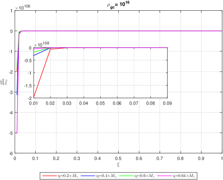
Figure 1: Case $1$: Perturbation through LDP. $\frac{\delta R_{1}}{\delta\rho_{gc}}$ as a function of $\xi$ for $n=1,~{}\alpha=8\times 10^{-11},~{}\alpha_{1}=0.2$, red curve: q=0.2 $M_{\odot}$, blue curve: q=0.4 $M_{\odot}$, green curve: q=0.6 $M_{\odot}$, magenta curve: q=0.64 $M_{\odot}$

.

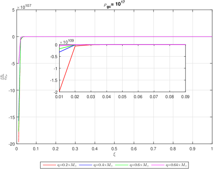
Figure 2: Case $1$: Perturbation through LDP. $\frac{\delta R_{1}}{\delta\rho_{gc}}$ as a function of $\xi$ for $n=1.5,~{}\alpha=2\times 10^{-10},~{}\alpha_{1}=0.5$, red curve: q=0.2 $M_{\odot}$, blue curve: q=0.4 $M_{\odot}$, green curve: q=0.6 $M_{\odot}$, magenta curve: q=0.64 $M_{\odot}$

.

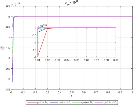
Figure 3: Case $1$: Perturbation through LDP. $\frac{\delta R_{1}}{\delta\rho_{gc}}$ as a function of $\xi$ for $n=1,~{}\alpha=0.5,~{}\alpha_{1}=0.8$, red curve: q=0.2 $M_{\odot}$, blue curve: q=0.4 $M_{\odot}$, green curve: q=0.6 $M_{\odot}$, magenta curve: q=0.64 $M_{\odot}$

.

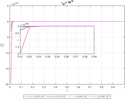
Figure 4: Case $2$: Perturbation through LDP. $\frac{\delta R_{2}}{\delta\rho_{gc}}$ as a function of $\xi$ for $n=1,~{}\alpha=8\times 10^{-11},~{}\alpha_{1}=0.2$, red curve: q=0.2 $M_{\odot}$, blue curve: q=0.4 $M_{\odot}$, green curve: q=0.6 $M_{\odot}$, magenta curve: q=0.64 $M_{\odot}$

.

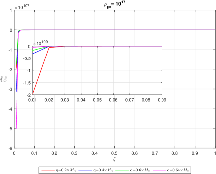
Figure 5: Case $2$: Perturbation through LDP. $\frac{\delta R_{2}}{\delta\rho_{gc}}$ as a function of $\xi$ for $n=1.5,~{}\alpha=2\times 10^{-10},~{}\alpha_{1}=0.5$, red curve: q=0.2 $M_{\odot}$, blue curve: q=0.4 $M_{\odot}$, green curve: q=0.6 $M_{\odot}$, magenta curve: q=0.64 $M_{\odot}$

.

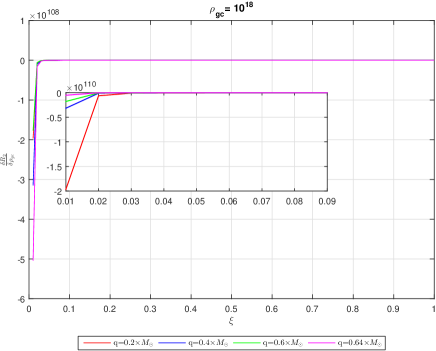
Figure 6: Case $2$: Perturbation through LDP. $\frac{\delta R_{2}}{\delta\rho_{gc}}$ as a function of $\xi$ for $n=1,~{}\alpha=0.5,~{}\alpha_{1}=0.8$, red curve: q=0.2 $M_{\odot}$, blue curve: q=0.4 $M_{\odot}$, green curve: q=0.6 $M_{\odot}$, magenta curve: q=0.64 $M_{\odot}$

.

4 Effect of Parametric Perturbation

In this section, we will study the stability of charged polytropes by perturbing the polytropic index and anisotropy factor. For this purpose we assume that our distribution satisfy the following relation

$$\Delta=C(\rho+P_{r})\Big{[}\frac{4\pi r^{4}P_{r}-q^{2}+mr}{r^{2}-2mr+q^{2}}\Big{]},$$ (34)

where $C$ is constant, producing the following form of HEe

$$R_{3}=\frac{dP_{r}}{dr}+h(\rho+P_{r})\Big{(}\frac{4\pi r^{4}P_{r}-q^{2}+mr}{r(r^{2}-2mr+q^{2})}\Big{)}-\frac{q}{4\pi r^{4}}\frac{dq}{dr},$$ (35)

with $h=1-2C$. Now we shall briefly review the main results for each case.

4.1 Case 1

Let the perturbation be carried out through polytropic model parameters

$$n\longrightarrow\tilde{n}+\delta n,~{}~{}~{}q\longrightarrow\tilde{q}+\delta q,~{}~{}~{}h\longrightarrow\tilde{h}+\delta h,$$ (36)

assuming that radial pressure remain same after perturbation, then from Eq.$(\ref{14})$ we can write

$$\tilde{P_{r}}=P_{r}=\alpha_{1}\rho_{gc}\theta^{n}+K\rho_{gc}^{1+\frac{1}{n}}\theta^{1+n}.$$ (37)

Also from Eq.$(\ref{15})$

$$\tilde{\rho}=\rho_{gc}\theta^{1+\tilde{n}}+\tilde{n}P_{r}.$$ (38)

Thus the perturb form of Eq.$(\ref{30})$ become

$$\hat{R_{3}}=\frac{dP_{r}}{dr}+\tilde{h}(\tilde{\rho}+P_{r})\Big{(}\frac{4\pi r^{4}P_{r}-q^{2}+\tilde{m}r}{r(r^{2}-2\tilde{m}r+q^{2})}\Big{)}-\frac{\tilde{q}}{4\pi r^{4}}\frac{d\tilde{q}}{dr}=0.$$ (39)

Now using Eqs.$(\ref{16})$, $(\ref{41})$ and $(\ref{42})$ in Eq.$(\ref{43})$, we get

$$\tilde{R_{3}}=(n\alpha_{1}\theta^{n-1}+\alpha_{3}\theta^{n})\frac{d\theta}{d\xi}-\frac{\alpha_{4}}{\alpha_{3}\tilde{q}\xi^{4}}\frac{d\tilde{q}}{d\xi}+\tilde{h}(\tilde{\theta^{n}}+(2\tilde{n}+1)$$

$$(\alpha_{1}\theta^{n}+\alpha\theta^{n+1}))\Big{(}\frac{(\alpha_{1}\theta^{n}+\alpha\theta^{n+1})\xi^{4}-\alpha_{3}^{-1}\alpha_{4}+\xi\tilde{v}(\xi)}{\alpha_{3}^{-1}\xi^{3}-2\tilde{v}(\xi)\xi^{2}-\alpha_{3}^{-1}\alpha_{4}\xi}\Big{)}.$$ (40)

From the above equation it follows up to first order, we may write

$$\delta\hat{R_{3}}=\hat{R_{3}}\Big{(}\xi,1+\delta n,h+\delta hv+\delta v,q+\delta q\Big{)},$$ (41)

$$\delta{R_{3}} = \Big{(}\frac{\partial{\tilde{R_{3}}}}{\partial\tilde{n}}\Big{)}\mathrel{\mathop{\Big{|}_{\tilde{n}=n,~{}\tilde{v}=v}}_{\mathrm{\tilde{h}=h,~{}\tilde{q}=q}}}\delta n+\Big{(}\frac{\partial{\tilde{R_{3}}}}{\partial\tilde{v}}\Big{)}\mathrel{\mathop{\Big{|}_{\tilde{n}=n,~{}\tilde{v}=v}}_{\mathrm{\tilde{h}=h,~{}\tilde{q}=q}}}\delta v$$ (42)

$$+\Big{(}\frac{\partial{\tilde{R_{3}}}}{\partial\tilde{h}}\Big{)}\mathrel{\mathop{\Big{|}_{\tilde{n}=n,~{}\tilde{v}=v}}_{\mathrm{\tilde{h}=h,~{}\tilde{q}=q}}}\delta h+\Big{(}\frac{\partial{\tilde{R_{3}}}}{\partial\tilde{q}}\Big{)}\mathrel{\mathop{\Big{|}_{\tilde{n}=n,~{}\tilde{v}=v}}_{\mathrm{\tilde{h}=h,~{}\tilde{q}=q}}}\delta q.$$

Now suppose that $\beta=\{-2v\xi^{2}+\frac{\xi^{3}}{\alpha_{3}}+\frac{\alpha_{4}}{\alpha_{3}}\xi\}^{-1}$ and using Eq. $(\ref{44})$, we obtained

$$\frac{\partial{\tilde{R_{3}}}}{\partial\tilde{n}}\mathrel{\mathop{\Big{|}_{\tilde{n}=n,~{}\tilde{v}=v}}_{\mathrm{\tilde{h}=h,~{}\tilde{q}=q}}} = \beta h(\theta^{n}\text{Log}[\theta]+2(\alpha\theta^{1+n}+\theta^{n}\alpha_{1}))(v\xi-\frac{\alpha_{4}}{\alpha_{3}}$$ (43)

$$+\xi^{4}(\alpha\theta^{1+n}+\theta^{n}\alpha_{1})),$$

$$\frac{\partial{\tilde{R_{3}}}}{\partial\tilde{v}}\mathrel{\mathop{\Big{|}_{\tilde{n}=n,~{}\tilde{v}=v}}_{\mathrm{\tilde{h}=h,~{}\tilde{q}=q}}}=\beta^{2}2h\xi^{2}(\theta^{n}+(1+2n)(\alpha\theta^{1+n}+\theta^{n}\alpha_{1}))(v\xi-\frac{\alpha_{4}}{\alpha_{3}}$$

$$+\xi^{4}(\alpha\theta^{1+n}+\theta^{n}\alpha_{1}))+\beta h\xi(\theta^{n}+(1+2n)(\alpha\theta^{1+n}+\theta^{n}\alpha_{1}))$$ (44)

$$\frac{\partial{\tilde{R_{3}}}}{\partial\tilde{h}}\mathrel{\mathop{\Big{|}_{\tilde{n}=n,~{}\tilde{v}=v}}_{\mathrm{\tilde{h}=h,~{}\tilde{q}=q}}} = \beta(\theta^{n}+(1+2n)(\alpha\theta^{1+n}+\theta^{n}\alpha_{1}))(v\xi-\frac{\alpha_{4}}{\alpha_{3}}$$ (45)

$$+\xi^{4}(\alpha\theta^{1+n}+\theta^{n}\alpha_{1})),$$

$$\frac{\partial{\tilde{R_{3}}}}{\partial\tilde{q}}\mathrel{\mathop{\Big{|}_{\tilde{n}=n,~{}\tilde{v}=v}}_{\mathrm{\tilde{h}=h,~{}\tilde{q}=q}}} = -\frac{8h\pi qP_{\text{rc}}}{\alpha_{3}^{2}\alpha}\Big{\{}\beta(\theta^{n}+(1+2n)(\alpha\theta^{1+n}+\theta^{n}\alpha_{1}))+$$ (46)

$$\beta^{2}\xi(\theta^{n}+(1+2n)(\alpha\theta^{1+n}+\theta^{n}\alpha_{1}))(v\xi-\frac{\alpha_{4}}{\alpha_{3}}+$$

$$\xi^{4}(\alpha\theta^{1+n}+\theta^{n}\alpha_{1}))\Big{\}}-\frac{4\pi P_{\text{rc}}\frac{dq}{d\xi}}{\alpha_{3}^{2}\alpha\xi^{4}}-\frac{4\pi qP_{\text{rc}}\frac{d^{2}q}{d\xi^{2}}}{\alpha_{3}^{2}\alpha\xi^{4}}.$$

Also From Eq.$(\ref{19})$, we have

$$\tilde{v}=\int_{0}^{\xi}\Big{[}\bar{\xi}^{2}\big{\{}\theta^{\tilde{n}}+\tilde{n}(\alpha_{1}\theta^{n}+\alpha\theta^{n+1})\big{\}}-\frac{\alpha_{4}}{\alpha_{3}\bar{\xi}^{2}}+\frac{\alpha_{4}}{\alpha_{3}\bar{\xi}q}\frac{dq}{d\xi}\Big{]}d\bar{\xi},$$ (47)

and

$$\delta v=F_{1}\delta n,~{}~{}~{}\delta q=\frac{F_{1}}{F_{2}}\delta n~{}~{}~{}\delta h=-\Gamma\delta n,$$ (48)

where

$$F_{1}=\int_{0}^{\xi}\bar{\xi}^{2}\big{\{}\theta^{\tilde{n}}log\theta+(\alpha_{1}\theta^{n}+\alpha\theta^{n+1})\big{\}}d\bar{\xi},$$

$$F_{2}=\int_{0}^{\xi}\frac{\alpha_{4}}{\alpha_{3}\bar{\xi}q}\Big{[}-\frac{1}{q\bar{\xi}}+\frac{dq}{d\xi}+q\frac{d^{2}q}{d\xi^{2}}\Big{]}d\bar{\xi},$$ (49)

and

$$\Gamma=\Bigg{(}\frac{F_{1}\frac{\partial\hat{\tilde{R}}}{\partial\tilde{v}}+F_{2}\frac{\partial\hat{\tilde{R}}}{\partial\hat{\tilde{q}}}+\frac{\partial\hat{\tilde{R}}}{\partial\tilde{n}}}{\frac{\partial\hat{\tilde{R}}}{\partial\tilde{h}}}\Bigg{)}\mathrel{\mathop{\Big{|}_{\tilde{n}=n,~{}\tilde{v}=v}}_{\mathrm{\tilde{h}=h,~{}\tilde{q}=q}}}.$$ (50)

So

$$\delta R_{3} = \Bigg{(}\beta h(\theta^{n}\text{Log}[\theta]+2(\alpha\theta^{1+n}+\theta^{n}\alpha_{1}))(v\xi-\frac{\alpha_{4}}{\alpha_{3}}+\xi^{4}(\alpha\theta^{1+n}+\theta^{n}\alpha_{1}))$$ (51)

$$- \Gamma\beta(\theta^{n}+(1+2n)(\alpha\theta^{1+n}+\theta^{n}\alpha_{1}))(v\xi-\frac{\alpha_{4}}{\alpha_{3}}+\xi^{4}(\alpha\theta^{1+n}+\theta^{n}\alpha_{1}))$$

$$+ F_{1}\Big{(}h\beta\xi(\theta^{n}+(1+2n)(\alpha\theta^{1+n}+\theta^{n}\alpha_{1}))+2h\beta^{2}\xi^{2}(\theta^{n}+(1+2n)$$

$$(\alpha\theta^{1+n}+\theta^{n}\alpha_{1}))(v\xi-\frac{\alpha_{4}}{\alpha_{3}}+\xi^{4}(\alpha\theta^{1+n}+\theta^{n}\alpha_{1}))\Big{)}$$

$$+ \frac{F_{1}}{F_{2}}\Big{(}-\frac{8h\pi qP_{\text{rc}}}{\alpha_{3}^{2}\alpha}\Big{(}\beta(\theta^{n}+(1+2n)(\alpha\theta^{1+n}+\theta^{n}\alpha_{1}))$$

$$+ \xi\beta^{2}(\theta^{n}+(1+2n)(\alpha\theta^{1+n}+\theta^{n}\alpha_{1}))(v\xi-\frac{\alpha_{4}}{\alpha_{3}}+\xi^{4}(\alpha\theta^{1+n}+\theta^{n}\alpha_{1}))\Big{)}$$

$$-\frac{4\pi P_{\text{rc}}\frac{dq}{d\xi}}{\alpha\alpha_{3}^{2}\xi^{4}}-\frac{4\pi qP_{\text{rc}}\frac{d^{2}q}{d\xi^{2}}}{\alpha\alpha_{3}^{2}\xi^{4}}\Big{)}\Bigg{)}\text{$\delta$n}.$$

It would be more convenient to use variable $x$ defined by

$$\xi=\bar{A}x,~{}~{}~{}\bar{A}=Ar_{\Sigma}=\xi_{\Sigma},$$ (52)

then

$$\delta R_{3} = \Bigg{(}\beta h(\theta^{n}\text{Log}[\theta]+2(\alpha\theta^{1+n}+\theta^{n}\alpha_{1}))(v(\bar{A}x)-\frac{\alpha_{4}}{\alpha_{3}}+(\bar{A}x)^{4}(\alpha\theta^{1+n}+\theta^{n}\alpha_{1}))$$ (53)

$$- \Gamma\beta(\theta^{n}+(1+2n)(\alpha\theta^{1+n}+\theta^{n}\alpha_{1}))(v(\bar{A}x)-\frac{\alpha_{4}}{\alpha_{3}}+(\bar{A}x)^{4}(\alpha\theta^{1+n}+\theta^{n}\alpha_{1}))$$

$$+ F_{1}\Big{(}h\beta(\bar{A}x)(\theta^{n}+(1+2n)(\alpha\theta^{1+n}+\theta^{n}\alpha_{1}))+2h\beta^{2}(\bar{A}x)^{2}(\theta^{n}+(1+2n)$$

$$(\alpha\theta^{1+n}+\theta^{n}\alpha_{1}))(v(\bar{A}x)-\frac{\alpha_{4}}{\alpha_{3}}+(\bar{A}x)^{4}(\alpha\theta^{1+n}+\theta^{n}\alpha_{1}))\Big{)}$$

$$+ \frac{F_{1}}{F_{2}}\Big{(}-\frac{8h\pi qP_{\text{rc}}}{\alpha_{3}^{2}\alpha}\Big{(}\beta(\theta^{n}+(1+2n)(\alpha\theta^{1+n}+\theta^{n}\alpha_{1}))$$

$$+ (\bar{A}x)\beta^{2}(\theta^{n}+(1+2n)(\alpha\theta^{1+n}+\theta^{n}\alpha_{1}))(v(\bar{A}x)-\frac{\alpha_{4}}{\alpha_{3}}+(\bar{A}x)^{4}(\alpha\theta^{1+n}+\theta^{n}\alpha_{1}))\Big{)}$$

$$-\frac{4\pi P_{\text{rc}}\frac{dq}{dx}}{\alpha\alpha_{3}^{2}\bar{A}^{5}x^{4}}-\frac{4\pi qP_{\text{rc}}\frac{d^{2}q}{dx^{2}}}{\alpha\alpha_{3}^{2}\bar{A}^{6}x^{4}}\Big{)}\Bigg{)}\text{$\delta$n}.$$

We will use above equation to plot the perturbed force $\frac{\delta R_{3}}{\delta n}$ against radius of star and observe it for possible occurrence of cracking (overturning) in polytropes of first kind developed under the GPEoS.

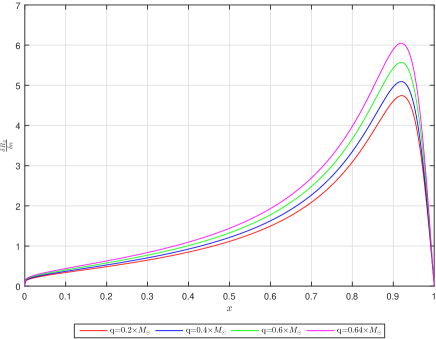
Figure 7: Case $1$: Perturbation through n, q and h. $\frac{\delta R_{3}}{\delta n}$ as a function of $x$ for $n=1,~{}\alpha=8\times 10^{-11},~{}\alpha_{1}=0.2,h=1.5,\Gamma=1.4$, red curve: q=0.2 $M_{\odot}$, blue curve: q=0.4 $M_{\odot}$, green curve: q=0.6 $M_{\odot}$, magenta curve: q=0.64 $M_{\odot}$

.

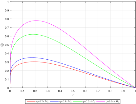
Figure 8: Case $1$: Perturbation through n, q and h. $\frac{\delta R_{3}}{\delta n}$ as a function of $x$ for $n=1,~{}\alpha=2\times 10^{-10},~{}\alpha_{1}=0.4,h=0.5,\Gamma=1.0$, red curve: q=0.2 $M_{\odot}$, blue curve: q=0.4 $M_{\odot}$, green curve: q=0.6 $M_{\odot}$, magenta curve: q=0.64 $M_{\odot}$

.

Figure 9: Case $1$: Perturbation through n, q and h. $\frac{\delta R_{3}}{\delta n}$ as a function of $x$ for $n=1,~{}\alpha=0.8,~{}\alpha_{1}=0.2,h=1.5,\Gamma=1.5$, red curve: q=0.2 $M_{\odot}$, blue curve: q=0.4 $M_{\odot}$, green curve: q=0.6 $M_{\odot}$, magenta curve: q=0.64 $M_{\odot}$

.

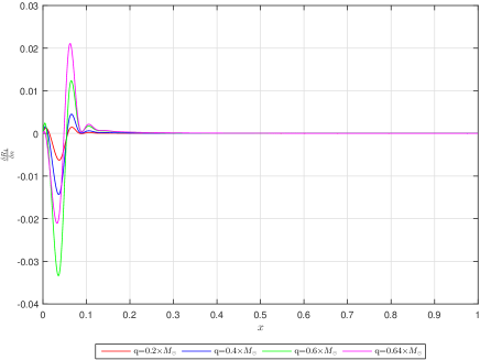
Figure 10: Case $2$: Perturbation through n, q and h. $\frac{\delta R_{4}}{\delta n}$ as a function of $x$ for $n=1,~{}\alpha=8\times 10^{-11},~{}\alpha_{1}=0.2,h=1.5,\Gamma=1.4$, red curve: q=0.2 $M_{\odot}$, blue curve: q=0.4 $M_{\odot}$, green curve: q=0.6 $M_{\odot}$, magenta curve: q=0.64 $M_{\odot}$

.

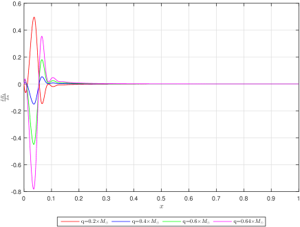
Figure 11: Case $2$: Perturbation through n, q and h. $\frac{\delta R_{4}}{\delta n}$ as a function of $x$ for $n=1,~{}\alpha=2\times 10^{-10},~{}\alpha_{1}=0.4,h=0.5,\Gamma=1.0$, red curve: q=0.2 $M_{\odot}$, blue curve: q=0.4 $M_{\odot}$, green curve: q=0.6 $M_{\odot}$, magenta curve: q=0.64 $M_{\odot}$

.

4.2 Case 2

Now we apply the parametric perturbation on polytropes of second kind here. So from Eq.$(\ref{30})$ can be written as

$$\tilde{P_{r}}=P_{r}=\alpha_{1}\rho_{c}\theta^{n}+K\rho_{c}^{1+\frac{1}{n}}\theta^{n+1}.$$ (54)

Now Eq.$(\ref{43})$ will transform as

$$\tilde{R_{4}}=(n\alpha_{1}\theta^{n-1}+\alpha_{3}\theta^{n})\frac{d\theta}{d\xi}-\frac{\alpha_{4}}{\alpha_{3}\tilde{q}\xi^{4}}\frac{d\tilde{q}}{d\xi}+\tilde{h}(\tilde{\theta^{n}}+\alpha_{1}\theta^{n}+\alpha\theta^{n+1})$$

$$\Big{(}\frac{(\alpha_{1}\theta^{n}+\alpha\theta^{n+1})\xi^{4}-\alpha_{3}^{-1}\alpha_{4}+\xi\tilde{v}(\xi)}{\alpha_{3}^{-1}\xi^{3}-2\tilde{v}(\xi)\xi^{2}-\alpha_{3}^{-1}\alpha_{4}\xi}\Big{)}.$$ (55)

From the above equation it follows up to first order, we may write

$$\delta\hat{R_{4}}=\hat{R_{4}}\Big{(}\xi,1+\delta n,h+\delta hv+\delta v,q+\delta q\Big{)},$$ (56)

$$\delta{R_{4}} = \Big{(}\frac{\partial{\tilde{R_{4}}}}{\partial\tilde{n}}\Big{)}\mathrel{\mathop{\Big{|}_{\tilde{n}=n,~{}\tilde{v}=v}}_{\mathrm{\tilde{h}=h,~{}\tilde{q}=q}}}\delta n+\Big{(}\frac{\partial{\tilde{R_{4}}}}{\partial\tilde{v}}\Big{)}\mathrel{\mathop{\Big{|}_{\tilde{n}=n,~{}\tilde{v}=v}}_{\mathrm{\tilde{h}=h,~{}\tilde{q}=q}}}\delta v$$ (57)

$$+\Big{(}\frac{\partial{\tilde{R_{4}}}}{\partial\tilde{h}}\Big{)}\mathrel{\mathop{\Big{|}_{\tilde{n}=n,~{}\tilde{v}=v}}_{\mathrm{\tilde{h}=h,~{}\tilde{q}=q}}}\delta h+\Big{(}\frac{\partial{\tilde{R_{4}}}}{\partial\tilde{q}}\Big{)}\mathrel{\mathop{\Big{|}_{\tilde{n}=n,~{}\tilde{v}=v}}_{\mathrm{\tilde{h}=h,~{}\tilde{q}=q}}}\delta q.$$

Then using Eq.$(\ref{59})$, we obtained

$$\frac{\partial{\tilde{R_{4}}}}{\partial\tilde{n}}\mathrel{\mathop{\Big{|}_{\tilde{n}=n,~{}\tilde{v}=v}}_{\mathrm{\tilde{h}=h,~{}\tilde{q}=q}}}=\beta h\theta^{n}\text{Log}[\theta](v\xi-\frac{4\pi q^{2}P_{\text{rc}}}{(1+n)^{2}\alpha^{3}}+\xi^{4}(\alpha\theta^{1+n}+\theta^{n}\alpha_{1})),$$ (58)

$$\frac{\partial{\tilde{R_{4}}}}{\partial\tilde{v}}\mathrel{\mathop{\Big{|}_{\tilde{n}=n,~{}\tilde{v}=v}}_{\mathrm{\tilde{h}=h,~{}\tilde{q}=q}}} = \beta h\xi(\theta^{n}+\alpha\theta^{1+n}+\theta^{n}\alpha_{1})+2\beta^{2}h\xi^{2}(\theta^{n}+\alpha\theta^{1+n}+\theta^{n}\alpha_{1})$$ (59)

$$(v\xi-\frac{4\pi q^{2}P_{\text{rc}}}{(1+n)^{2}\alpha^{3}}+\xi^{4}(\alpha\theta^{1+n}+\theta^{n}\alpha_{1})),$$

$$\frac{\partial{\tilde{R_{4}}}}{\partial\tilde{h}}\mathrel{\mathop{\Big{|}_{\tilde{n}=n,~{}\tilde{v}=v}}_{\mathrm{\tilde{h}=h,~{}\tilde{q}=q}}}=\beta(\theta^{n}+\alpha\theta^{1+n}+\theta^{n}\alpha_{1})(v\xi-\frac{\alpha_{4}}{\alpha_{3}}+\xi^{4}(\alpha\theta^{1+n}+\theta^{n}\alpha_{1})),$$ (60)

$$\frac{\partial{\tilde{R_{4}}}}{\partial\tilde{q}}\mathrel{\mathop{\Big{|}_{\tilde{n}=n,~{}\tilde{v}=v}}_{\mathrm{\tilde{h}=h,~{}\tilde{q}=q}}} = \frac{8h\pi qP_{\text{rc}}}{\alpha_{3}^{2}\alpha}\Big{\{}\beta(\theta^{n}+\alpha\theta^{1+n}+\theta^{n}\alpha_{1})-\xi\beta^{2}(\theta^{n}+\alpha\theta^{1+n}$$ (61)

$$+\theta^{n}\alpha_{1})(v\xi-\frac{4\pi q^{2}P_{\text{rc}}}{(1+n)^{2}\alpha^{3}}+\xi^{4}(\alpha\theta^{1+n}+\theta^{n}\alpha_{1}))\Big{\}}$$

$$-\frac{4\pi P_{\text{rc}}\frac{dq}{d\xi}}{(1+n)^{2}\alpha^{3}\xi^{4}}-\frac{4\pi qP_{\text{rc}}\frac{d^{2}q}{d\xi}^{2}}{(1+n)^{2}\alpha^{3}\xi^{4}}.$$

From Eq.$(\ref{33})$, we have

$$\tilde{v}=\int_{0}^{\xi}\Big{[}\bar{\xi}^{2}\theta^{\tilde{n}}-\frac{\alpha_{4}}{\alpha_{3}\bar{\xi}^{2}}+\frac{\alpha_{4}}{\alpha_{3}\bar{\xi}q}\frac{dq}{d\xi}\Big{]}d\bar{\xi},$$ (62)

and

$$\delta v=F_{3}\delta n,~{}~{}~{}\delta q=\frac{F_{3}}{F_{2}}\delta n~{}~{}~{}\delta h=-\Gamma\delta n,$$ (63)

where

$$F_{3}=\int_{0}^{\xi}\bar{\xi}^{2}\theta^{\tilde{n}}log\theta d\bar{\xi},$$ (64)

and

$$\Gamma=\Bigg{(}\frac{F_{3}\frac{\partial\hat{\tilde{R}}}{\partial\tilde{v}}+F_{2}\frac{\partial\hat{\tilde{R}}}{\partial\hat{\tilde{q}}}+\frac{\partial\hat{\tilde{R}}}{\partial\tilde{n}}}{\frac{\partial\hat{\tilde{R}}}{\partial\tilde{h}}}\Bigg{)}\mathrel{\mathop{\Big{|}_{\tilde{n}=n,~{}\tilde{v}=v}}_{\mathrm{\tilde{h}=h,~{}\tilde{q}=q}}}.$$ (65)

So

$$\delta R_{4} = \Bigg{(}\beta h\theta^{n}\text{Log}[\theta](v\xi-\frac{\alpha_{4}}{\alpha_{3}}+\xi^{4}(\alpha\theta^{1+n}+\theta^{n}\alpha_{1}))-\beta\Gamma(\theta^{n}+\alpha\theta^{1+n}$$ (66)

$$+\theta^{n}\alpha_{1})(v\xi-\frac{\alpha_{4}}{\alpha_{3}}+\xi^{4}(\alpha\theta^{1+n}+\theta^{n}\alpha_{1}))+F_{3}\Big{(}h\beta\xi(\theta^{n}+\alpha\theta^{1+n}$$

$$+\theta^{n}\alpha_{1})+2\beta^{2}h\xi^{2}(\theta^{n}+\alpha\theta^{1+n}+\theta^{n}\alpha_{1})(v\xi-\frac{\alpha_{4}}{\alpha_{3}}+\xi^{4}(\alpha\theta^{1+n}$$

$$+\theta^{n}\alpha_{1}))\Big{)}+\frac{F_{3}}{F_{2}}\Big{(}\frac{8h\pi qP_{\text{rc}}}{\alpha_{3}^{2}\alpha}\Big{(}\beta(\theta^{n}+\alpha\theta^{1+n}+\theta^{n}\alpha_{1})-\xi\beta^{2}(\theta^{n}$$

$$+\alpha\theta^{1+n}+\theta^{n}\alpha_{1})(v\xi-\frac{4\pi q^{2}P_{\text{rc}}}{(1+n)^{2}\alpha^{3}}+\xi^{4}(\alpha\theta^{1+n}+\theta^{n}\alpha_{1}))\Big{)}$$

$$-\frac{4\pi P_{\text{rc}}\frac{dq}{d\xi}}{(1+n)^{2}\alpha^{3}\xi^{4}}-\frac{4\pi qP_{\text{rc}}\frac{d^{2}q}{d\xi^{2}}}{(1+n)^{2}\alpha^{3}\xi^{4}}\Big{)}\Bigg{)}\text{$\delta$n}.$$

It would be more convenient to use variable $x$ defined by

$$\xi=\bar{A}x,~{}~{}~{}\bar{A}=Ar_{\Sigma}=\xi_{\Sigma},$$ (67)

then

$$\delta R_{4} = \Bigg{(}\beta h\theta^{n}\text{Log}[\theta](v(\bar{A}x)-\frac{\alpha_{4}}{\alpha_{3}}+(\bar{A}x)^{4}(\alpha\theta^{1+n}+\theta^{n}\alpha_{1}))-\beta\Gamma(\theta^{n}+\alpha\theta^{1+n}$$ (68)

$$+\theta^{n}\alpha_{1})(v(\bar{A}x)-\frac{\alpha_{4}}{\alpha_{3}}+(\bar{A}x)^{4}(\alpha\theta^{1+n}+\theta^{n}\alpha_{1}))+F_{3}\Big{(}h\beta(\bar{A}x)(\theta^{n}+\alpha\theta^{1+n}$$

$$+\theta^{n}\alpha_{1})+2\beta^{2}h(\bar{A}x)^{2}(\theta^{n}+\alpha\theta^{1+n}+\theta^{n}\alpha_{1})(v(\bar{A}x)-\frac{\alpha_{4}}{\alpha_{3}}+(\bar{A}x)^{4}(\alpha\theta^{1+n}$$

$$+\theta^{n}\alpha_{1}))\Big{)}+\frac{F_{3}}{F_{2}}\Big{(}\frac{8h\pi qP_{\text{rc}}}{\alpha_{3}^{2}\alpha}\Big{(}\beta(\theta^{n}+\alpha\theta^{1+n}+\theta^{n}\alpha_{1})-(\bar{A}x)\beta^{2}(\theta^{n}$$

$$+\alpha\theta^{1+n}+\theta^{n}\alpha_{1})(v(\bar{A}x)-\frac{4\pi q^{2}P_{\text{rc}}}{(1+n)^{2}\alpha^{3}}+(\bar{A}x)^{4}(\alpha\theta^{1+n}+\theta^{n}\alpha_{1}))\Big{)}$$

$$-\frac{4\pi P_{\text{rc}}\frac{dq}{dx}}{(1+n)^{2}\alpha^{3}\bar{A}^{5}x^{4}}-\frac{4\pi qP_{\text{rc}}\frac{d^{2}q}{dx^{2}}}{(1+n)^{2}\alpha^{3}\bar{A}^{6}x^{4}}\Big{)}\Bigg{)}\text{$\delta$n}.$$

We will use above equation to plot the perturbed force $\frac{\delta R_{4}}{\delta n}$ against radius of star and observe it for possible occurrence of cracking (overturning) in polytropes of first kind developed under the GPEoS.

5 Conclusion and Discussion

In this work, we have applied two different perturbation schemes on two types of charged polytropes developed under the assumption of GPEoS [30]. In first perturbation scheme, we have used LDP scheme with conformally flat condition and sketched the force distribution function against radius of star. Here, we have assumed that all physical parameters involved in the model and their derivatives as function of central density. Figure 1-3 show the plot of force distribution function $\frac{\delta R_{1}}{\delta\rho_{gc}}$ against dimension less radius $\xi$. It is observed that for different values of central density and charge the system remain stable even after perturbation. These plots represent a picture of system just after perturbation. We observe rapid growth in the perturbed force near the center but it become consistent, stable and smooth as we move from center to outer surface of star. The zoom box inside the figure depicted perturbed forces near the center. It clearly indicated that the as the magnitude of charge increases gradually the peak of perturbed forces become less comparatively and it indicates that the presence charge stabilized the system after perturbation. Such behavior is observed in both types of polytropes under LDP scheme (see figs. 1-6).

In second perturbation scheme, we have perturbed the system through parameters involved in the model like charge, anisotropy and polytropic index. Such perturbation is carried out with the assumption that radial pressure remain same even after perturbation. Under this perturbation scheme, the perturbed force distribution $\frac{\delta R_{3}}{\delta n}$ is plotted against radius of star (see 7-9). We get stable regions for small values of $\alpha$ as shown in 7 and 8. These plots also shows that the system is very sensitive towards the choice of parameters. Initially the perturbed force $\frac{\delta R_{3}}{\delta n}$ strong behavior near the boundary of star (see Figure 7) but slightly change in parameters shifts the magnitude of force towards the center of star (see Figure 8). In figs. 7 and 8 stable configurations are observed. If the value of $\alpha$ is increased significantly then the system become unstable after perturbation and cracking (overturning) is observed. For smaller values of charge weak cracking near the center and strong overturning occurs in the outer region. For sufficiently high value of charge we observe weak overturning near the center and strong cracking in the outer regions as shown in fig. 9. Under parametric perturbation the second kind of polytropes did not show any stable region and remain unstable under different combinations of parametric values. Cracking and overturning is observed in polytropes of second type as shown in 10 and 11.

From the above discussion, it is concluded that charged polytropes developed under GPEoS remain stable if LDP scheme is applied under conformally flat condition. They are not sensitive towards the perturbation in central density and such behavior appeared in both types discussed in this work. When perturbation is carried out through parameters, then first kind of polytropes show stable behavior for small values of $\alpha$ in the presence of charge but cracking (overturning) also appeared in this case for larger values. Further the second kind of polytropes remain unstable under under parametric perturbation. Hence the proper choice of parameters is very crucial in the study of polytropic models.

References

- [1] Chandrasekhar, S.: An introduction to the Study of Stellar Structure, University of Chicago, Chicago, (1939)
- [2] Tooper, R. F.: Astrophys. J. 140, 434 (1964)
- [3] Tooper, R. F.: Astrophys. J. 142, 1541 (1965)
- [4] Kovetz, A.: Astrophys. J. 154, 999 (1968)
- [5] Abramowicz, M. A.: Acta Astronomica 33, 313 (1983)
- [6] Bekenstein, J. D.: Phys. Rev. D 4, 2185 (1960)
- [7] Bonnor, W. B.: Zeit. Phys. 160, 59 (1960)
- [8] Bonnor, W. B.: Mon. Not. R. Astron. Soc. 129, 443 (1964)
- [9] Bondi, H.: Proc. R. Soc. Lond. A 281, 39 (1964)
- [10] Ray, S., Malheiro, M., Lemos, J.P.S., Zanchin, V.T.: Braz. J. Phys. 34, 310 (2004)
- [11] Herrera, L., Di Prisco, A., Ibanez, J.: Phys. Rev. D 84, 107501 (2011)
- [12] Takisa, P. M., Maharaj, S. D.: Astrophys. Space Sci. 45, 1951 (2013)
- [13] Cosenza, M., Herrera, L., Esculpi, M., Witten. L.: J. Math. Phys. 22, 118 (1981)
- [14] Herrera, L., Santos, N. O.: Phys. Rep. 286, 53 (1997)
- [15] Herrera, L., Barreto, W.: Gen. Rel. Grav. 36, 127 (2004)
- [16] Herrera, L., Di Prisco, A., Martin, J., Ospino, J., Santos, N. O., Troconis, O.: Phys. Rev. D 69, 084026 (2004).
- [17] Herrera, L., Barreto, W.: Phys. Rev. D 87, 087303 (2013)
- [18] Herrera, L., Barreto, W.: Phys. Rev. D 88, 084022 (2013)
- [19] Herrera, L., Di Prisco, A., Barreto, W., Ospino, J.: Gen. Rel. Grav. 46, 1827 (2014)
- [20] Bondi, H.: Proc. Roy. Soc. Lond. A 282, 303 (1964)
- [21] Herrera, L.: Phys. Lett. A 165, 206 (1992)
- [22] Gonzalez, G.A., Navarro, A., Nunez, L.A.: arXiv: 1410.7733.
- [23] Gonzalez, G.A., Navarro, A., Nunez, L.A.: J. Phys. Conf. Ser. 600(2015)012014.
- [24] Azam, M., Mardan, S. A., Rehman, M. A.: Astrophys. Space Sci. 358, 6 (2015)
- [25] Azam, M., Mardan, S. A., Rehman, M. A.: Astrophys. Space Sci. 359, 14 (2015)
- [26] Azam, M., Mardan, S. A., Rehman, M. A.: Adv. High Energy Phys. 2015, 865086 (2015)
- [27] Azam, M., Mardan, S. A., Rehman, M. A.: Commun. Theor. Phys. 65, 575 (2016)
- [28] Azam, M., Mardan, S. A., Rehman, M. A.: Chin. Phys. Lett. 33, 070401 (2016)
- [29] Sharif, M., Sadiq, S.: Can. J. Phys. 93, 1420 (2015)
- [30] Azam, M., Mardan, S.A., Noureen, I. et al.: Eur. Phys. J. C 76, 315 (2016)
- [31] Azam, M., Mardan, S.A., Noureen, I. et al.: Eur. Phys. J. C 76, 510 (2016)
- [32] Herrera, L., Fuenmayor, E., A., Leon, P.: Phys. Rev. D 93, 024247 (2016)
- [33] Sharif, M., Sadiq, S.: Eur. Phys. J. C 76, 568 (2016)
- [34] Azam, M., Mardan, S.A.: arXiv:1612.00290 [physics.gen-ph]
- [35] Darmois, G.: Memorial des Sciences Mathematiques, Fasc. 25 (Gautheir-Villars, 1927)
- [36] Israel, W.: Nuovo Cimento B 44S10 1 (1966); ibid. Erratum B48, 463 (1967)
- [37] Misner, C. W., Sharp, D. H.: Phys. Rev. 136, B571 (1964)