sectioning \setkomafonttitle
FFT-based homogenization on periodic anisotropic translation invariant spaces
Abstract
In this paper we derive a discretisation of the equation of quasi-static elasticity in homogenization in form of a variational formulation and the so-called Lippmann-Schwinger equation, in anisotropic spaces of translates of periodic functions. We unify and extend the truncated Fourier series approach, the constant finite element ansatz and the anisotropic lattice derivation. The resulting formulation of the Lippmann-Schwinger equation in anisotropic translation invariant spaces unifies and analyses for the first time both the Fourier methods and finite element approaches in a common mathematical framework. We further define and characterize the resulting periodised Green operator. This operator coincides in case of a Dirichlet kernel corresponding to a diagonal matrix with the operator derived for the Galerkin projection stemming from the truncated Fourier series approach and to the anisotropic lattice derivation for all other Dirichlet kernels. Additionally, we proof the boundedness of the periodised Green operator. The operator further constitutes a projection if and only if the space of translates is generated by a Dirichlet kernel. Numerical examples for both the de la Vallée Poussin means and Box splines illustrate the flexibility of this framework.
Keywords: homogenization, anisotropic lattices, translation invariant spaces,
Lippmann-Schwinger equation
MSC 2000: 42B35, 42B37, 65T40, 74B05, 74E30
1 Introduction
Many modern tools and products use composites, i.e. mixtures of two or more materials with distinct elastic properties to obtain certain flexible behaviour, dampening effects, or longevity. Homogenization aims to simplify simulations by replacing the microscopically composed material by a homogeneous one which behaves the same on the macroscopic scale. Mathematically one assumes is a periodic microstructure, i.e. a structure that can be represented by a certain unit cell with periodic boundary conditions.
For the simulation of such elastic composite structures Moulinec and Suquet [18, 18] derive an algorithm based on the fast Fourier transform. This algorithm, called the Basic Scheme, inspired many similar numerical approaches based on using discretised differential operators [28, 23, 22] and extensions to porous media [15, 22]. Information on sub-structures of the geometry is incorporated into the solution method in [12]. The Basic Scheme is generalized to problems of higher order, i.e. derivatives of strain and stiffness [26], and the solution of the arising linear system by Krylov subspace methods is analysed in [29].
Vondřejc et.al. [27] show that the method of Moulinec and Suquet can also be understood as a Galerkin projection using truncated Fourier series. This idea is generalized in [3] to anisotropic lattices thus allowing to take directional information on the geometrical structure or the orientation of interfaces between materials into account. Brisard and Dormieux [8, 9] use constant finite elements to arrive at the Basic Scheme with a modified linear operator, based on an energy based formulation.
In this paper we unify and extend the approaches of Vondřejc et.al., Brisard and Dormieux, and the anisotropic lattice ansatz obtaining a discretisation of the equations for quasi-static elasticity in homogenization in anisotropic spaces of periodic translates. Vondřejc et.al. show that a variational equation and a formulation with the strain as a fixed-point, the so-called Lippmann-Schwinger equation, are equivalent by means of a projection operator derived from the Green operator. This paper introduces a periodised Green operator on the space of translates for the Lippmann-Schwinger equation. Furthermore we classify the properties of this operator in case of spaces of translates and prove that it induces a projection operator if and only if the space of translates is generated by the Dirichlet kernel. Hence the (anisotropic) truncated Fourier series emerges as a case with special properties of the general setting introduced here. This introduces further insight into the equivalence of the variational and the Lippmann-Schwinger equation formulation of Vondřejc et.al. The mathematical framework this paper introduces unifies and analyses the approaches of Fourier methods and finite elements for the first time. Especially using translates of Box splines [6] as ansatz functions incorporates the constant finite elements of Brisard and Dormieux allowing also for anisotropic finite elements of arbitrary smoothness. A different approach to solve the equation using linear finite elements with full quadrature is shown in [22] and is based on replacing the continuous differential operator by a discrete one.
Spaces of translates can for example be generated by de la Vallée Poussin means which provide a generalization of the Dirichlet and Fejér kernel. They combine a finite support in frequency domain with good localization in space [11]. These functions introduce a trade off between damping of the Gibbs phenomenon and reproduction of multivariate trigonometric monomials. They allow for better predictions of the elastic macroscopic properties of the composite material and result in smoother — and thus better — solutions. Further, different Box splines and their influence on the solution are demonstrated.
The remainder of the paper is structured as follows. After reviewing important properties of anisotropic spaces of translates in Section 2 the partial differential equation of quasi-static elasticity in homogenization is introduced in Section 3. Then, the periodised Green operator on spaces of translates is introduced. This operator is subsequently analysed regarding its equivalence to a projection operator and then used to discretise the Lippmann-Schwinger equation. Numerical examples are then provided in Section 4 and a conclusion is drawn in Section 5.
2 Preliminaries
Throughout this paper we will employ the following notation: the symbols , and denote scalars, vectors, and matrices, respectively. The only exception from this are which are reserved for functions. We denote the inner product of two vectors by and reserve the symbol for inner products of two functions or two generalized sequences, respectively. For a complex number , , we denote the complex conjugate by . Constants like Euler’s number or the imaginary unit , i.e. , are set upright.
Usually, we are concerned with -dimensional data, where , but the theory is written in arbitrary dimensions. Sets are denoted by capital case calligraphic letters, e.g. or and the same for the Fourier transform which all might depend on parameters given in round brackets. We denote second-order tensors by small Greek letters as with entries are indexed again by scalars and similarly we denote fourth-order tensors by capital calligraphic letters, where is the most prominent one.
2.1 Arbitrary patterns and the Fourier transform
The space of functions we are concerned with is the Hilbert space of (equivalence classes of) square integrable functions on the -dimensional torus with inner product
In several cases, the functions of interest are tensor-valued. For these functions, we take the tensor product of the Hilbert space, e.g. for the space of functions that have values being -dimensional matrices. The following preliminaries can be generalized to these tensor product spaces by performing the operations element wise. We restrict the following of this subsection therefore to the case of .
Every function can be written in its Fourier series representation
| (1) |
introducing the multivariate Fourier coefficients , . The equality in (1) is meant in sense. We denote by generalized sequences which form a Hilbert space with the inner product
The Parseval equation reads
| (2) |
The pattern and the generating set.
For any regular matrix we define the congruence relation for with respect to by
We define the lattice
and the pattern as any set of congruence representants of the lattice with respect to , e.g. or . For the rest of the paper we will refer to the set of congruence class representants in the symmetric unit cube . The generating set is defined by for any pattern . For both, the number of elements is given by which follows directly from [6, Lemma II.7].
For a regular integer matrix and an absolutely summable generalized sequence we further define the bracket sum
| (3) |
The bracket sum is periodic with respect to , i.e., holds for any .
A fast Fourier transform on patterns.
The discrete Fourier transform on the pattern is defined [10] by
| (4) |
where indicate the rows and indicate the columns of the Fourier matrix . The discrete Fourier transform on is defined for a vector arranged in the same ordering as the columns in (4) by
| (5) |
where the resulting vector is ordered as the columns of in (4). Its implementation yields complexity of similar to the classical Fourier transform, when the ordering is fixed as described in [1, Theorem 2]. Note that for the so-called rank-1-lattices, the Fourier transform on the pattern even reduces to a one-dimensional FFT for patterns in arbitrary dimensions [13].
2.2 Translation invariant spaces of periodic functions
Spaces of translates and interpolation.
A space of functions is called -invariant, if for all and all functions the translates . Especially the space
of translates of is -invariant. A function is of the form
For an easy calculation on the Fourier coefficients using the unique decomposition of into , , yields, that holds if and only if [14, Theorem 3.3]
| (6) |
holds, where denotes the discrete Fourier transform of , see [14]. Using the space of trigonometric polynomials on the generating set , which is denoted by
we define for a function the Fourier partial sum by
The discrete Fourier coefficients of a function that is evaluated pointwise on the pattern are defined by
The discrete Fourier coefficients are related to the Fourier coefficients for a function , where denotes the Wiener Algebra, i.e. the space of functions with absolutely convergent Fourier series. This relation is given in the following Lemma, also known as the aliasing formula, see e.g. [4, Lemma 2].
Lemma 2.1.
Let and the regular matrix be given. Then the discrete Fourier coefficients are given by
When looking at the space of translates, the following definition is crucial in order to approximate a function by using these translates.
Definition 2.2.
Let be a regular matrix. A function is called fundamental interpolant or Lagrange function of if
The following lemma characterizes the existence of such a fundamental interpolant in a space of translates and collects some properties of the translates themselves, see [2, Lemma 1.23] and [4, Lemma 2].
Lemma 2.3.
Given a regular matrix and a function , then the following holds.
-
a)
The fundamental interpolant exists if and only if
If the fundamental interpolant exists, it is uniquely determined.
-
b)
The set of translates is linear independent if and only if
-
c)
The set of translates is an orthonormal basis of if and only if
-
d)
Given a function we can obtain a function fulfilling
provided that the fundamental interpolant exists (which also implies linear independence of the translates on ) as
where the coefficients yield in Fourier coefficients by (6).
By using Lemma 2.3 changing from sampling values, i.e. the coefficients on the pattern of the fundamental interpolant, to coefficients with respect to in the corresponding space of translates can be done by using the Fourier transform (5) and the Fourier coefficients of .
For the remainder of this paper, two special spaces of translates are of interest, the periodised Box splines and the de la Vallée Poussin means.
Periodised Box splines.
Let denote a set of column vectors , , where we assume that these vectors span the , i.e. especially we have . Then the centred Box spline can be defined via its Fourier transform as
cf. [6, p. 11]. A Box spline has compact support. For a function we can introduce its periodisation
Its Fourier coefficients can be directly computed from the continuous Fourier transform of , cf. e.g. [4, p. 41], as
We combine these two to introduce the periodised Box Spline via its Fourier coefficients as
Finally, we obtain by scaling the periodised pattern Box Spline
Note that its translates might not be linearly independent for an arbitrary set of vectors in , see also [20]. However, by [4], see also [7, Sect. 4], the matrices of the form , , and , where at least two of the values are larger than , induce a periodised pattern Box spline with linear independent translates.
De la Vallée Poussin means.
A special case of -invariant spaces are the ones defined via de la Vallée Poussin means, following the construction of [5]. We call a function admissible if the function fulfils
-
a)
for all ,
-
b)
for ,
-
c)
for all .
This can be for example the Box splines of the form
where is the -dimensional unit matrix. In the following we define the de la Vallée Poussin means as follows, which is a special case of [5, Definition 4.2] setting therein.
Definition 2.4.
Let be a regular matrix and be an admissible function. The function , which is defined by their Fourier coefficients as
is called de la Vallée Poussin mean.
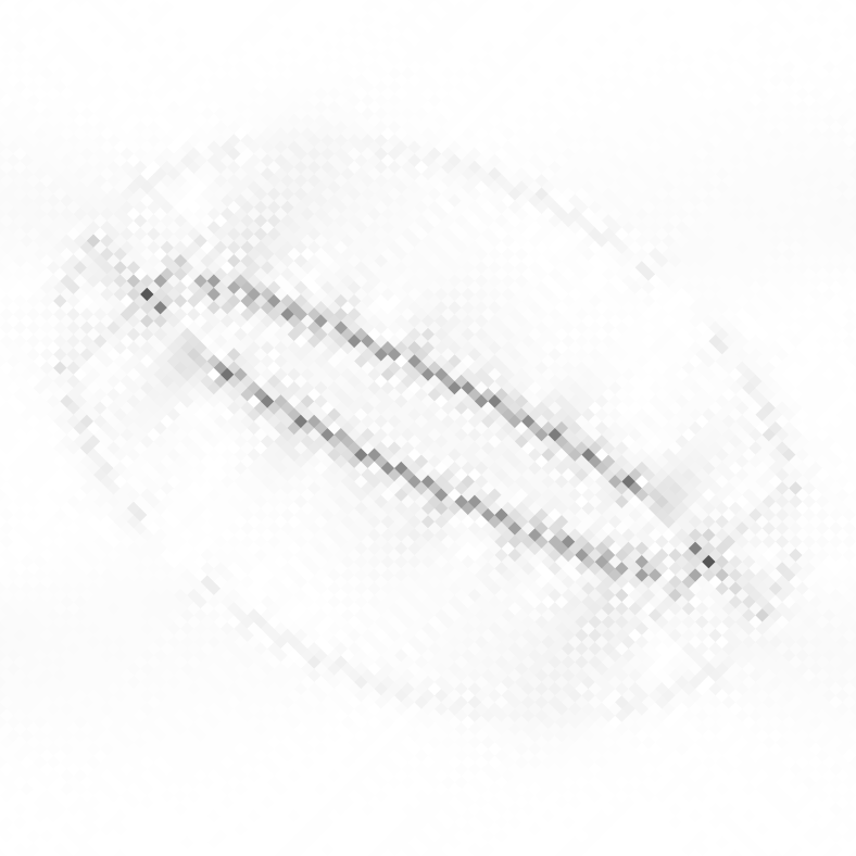
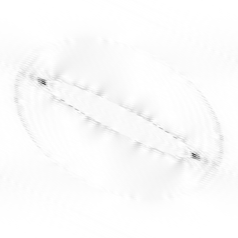
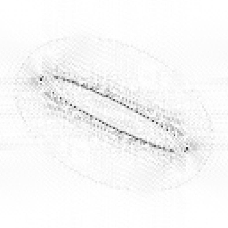
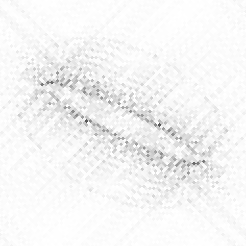
In case of Box splines this generalizes the one-dimensional de la Vallée Poussin means from [24, 21] to arbitrary patterns including the tensor product case for diagonal matrices , which where for example used in [25]. We will use the short hand notation and omit whenever its clear from the context. It is easy to see, that by admissibility of the fundamental interpolant exists for any de la Vallée Poussin mean . The functions generalize the classical de la Vallée Poussin means to higher dimensions and anisotropic patterns, for which examples are shown in Figure 1 and explained in the following.
Finally, the Dirichlet kernel is defined by using the function with
This kernel is comprised in the definition of the generalized de la Vallée Poussin mean as well. Furthermore we obtain the modified Dirichlet Kernel as a limiting case of the de la Vallée Poussin case.
As an example we choose and . For we obtain the usual rectangular (pixel grid) pattern while models a certain anisotropy, cf. [3, Fig. 2.1]. By further setting we obtain the de la Vallée Poussin means and . Their Fourier coefficients and after orthonormalising the translates, cf. Lemma 2.3 c), are shown in Figs. 1 1 (a) and 1 (b), respectively. Note that the first results in translates, while the second determinant is smaller and results in translates. The functions in time domain are plotted in Figs. 1 1 (c) and 1 (d), respectively. While the first can also be obtained by a tensor product of one-dimensional de la Vallée Poussin means, cf., e.g. [24], the second one prefers in time domain certain directions due to its anisotropic form.
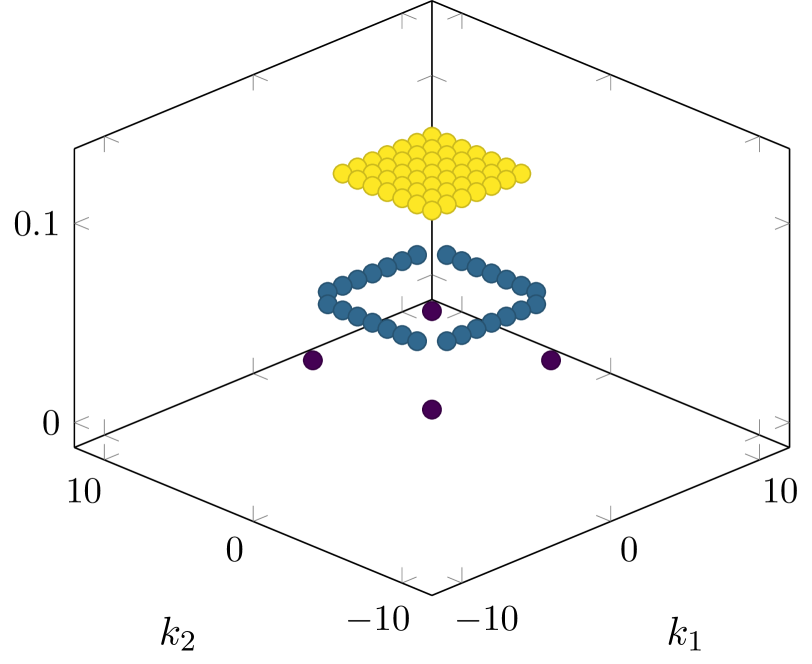
, .
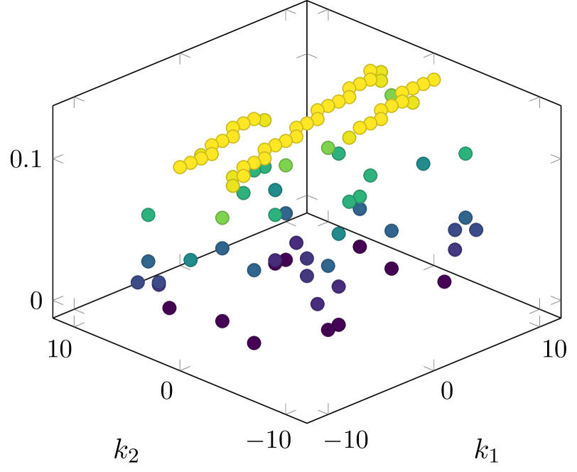
, .
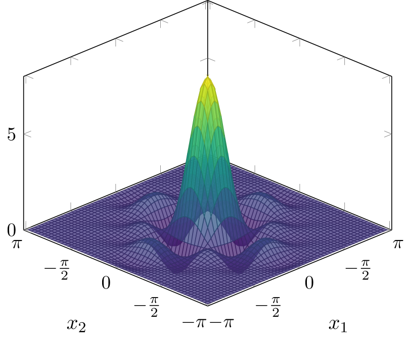
, .
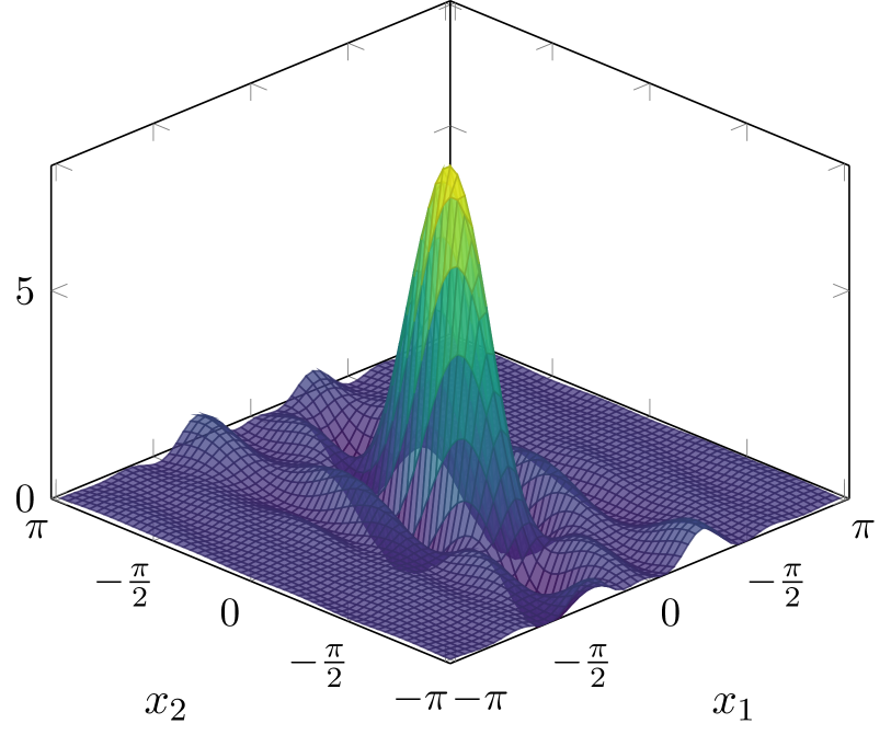
, .
3 Homogenization on spaces of translates
In the following steps we use anisotropic spaces of translates to discretise the quasi-static equation of linear elasticity in homogenization. First we introduce the necessary spaces and differential operators. With these we can state the partial differential equation we are interested in and two equivalent formulations, a variational equation and the so-called Lippmann-Schwinger equation. These formulations make use of the Green operator . Based on this operator we introduce the periodised Green operator and subsequently analyse its properties and special cases. Next we use this operator to discretise the partial differential equation while splitting the derivation into two steps.
3.1 The elasticity problem in periodic homogenization
FFT-based methods for the equations of linear elasticity in homogenization based on the Lippmann-Schwinger equation are first introduced by Moulinec and Suquet [18, 19]. Based on their method, Vondřejc et. al. [27] interpret the resulting discretisation as a Galerkin projection using trigonometric sums.
In the following we generalize the interpretation using trigonometric sums to spaces of translates of a periodic function. Therein the trigonometric sums will appear as a special case, namely when choosing the Dirichlet kernel’s translates and a diagonal matrix .
Let be an arbitrary set, then we introduce the notations
The space corresponds to symmetric matrices built of elements of and corresponds to fourth-order tensors with minor and major symmetries, i.e. .
We endow the space of symmetric matrices with the Frobenius inner product
We call a function uniformly elliptic if there exist constants such that for almost all functions it holds true that
A uniformly elliptic and constant function can be identified with an element from and is called elliptic in the following.
The Sobolev space is defined via Fourier series, i.e.
| with the norm | ||||
To simplify the equations of linear elasticity and the differential operators occurring therein we additionally introduce for the symmetrized gradient operator
| (7) |
and the divergence operator as the formal -adjoint of . The action of the symmetrized gradient operator in Fourier space is for given by
The basic solution space for the PDE we want to analyse is given by symmetric gradient fields with zero mean
With these preparations we can now state the partial differential equation describing quasi-static linear elasticity in homogenization.
Definition 3.1.
Let be uniformly elliptic and let be given. We want to find the strain such that
| (8) |
holds for all . With we hereby denote the product of the fourth-order stiffness tensor and the second-order strain , the symmetry making the order of multiplication irrelevant.
The stiffness distribution describes the material behaviour and is in practical applications usually a piece-wise constant function. The role of the macroscopic strain is that of an overall strain that is applied to the composed material and corresponds to pulling (or compressing) the composite in a certain direction.
For applications one is interested either in the strain field —or derivates like stress or displacements, respectively— or in the so-called effective stiffness of the medium. The overall stiffness behaviour of the composite given by the action of on is defined by
where is the solution of (8) corresponding to .
The space of suitable ansatz functions is in practice difficult to work with, especially regarding the discretisation steps that follow. A method to deal with that is introduced by Vondřejc et. al. [27]. They derive a projection operator with -adjoint that maps onto and thus replaces the structurally complicated space by a simpler one necessitating a more involved PDE. The operator acts as a second order derivative of a preconditioner that solves the constant coefficient PDE . For a derivation of the formula see for example [18, 19, 22].
Definition 3.2.
For a constant elliptic reference stiffness define the Green operator which acts as a Fourier multiplier. Its action on a field is given by the equation
| (9) | ||||
| with equality in -sense and Fourier coefficients | ||||
This operator allows to reformulate (8) with test functions in by projecting them onto the required function space. Further, this additional operator is easy do apply as it acts as a convolution operator, i.e. a Fourier multiplier.
Proposition 3.3.
Let , then fulfils
for all if and only if
| (10) |
holds true for all .
Proof.
For a proof see [27, Proposition 3]. ∎
By the properties of the operator this equation is equivalent to the so-called Lippmann-Schwinger equation with fixed point , cf.[27, Lemma 2]:
Proposition 3.4.
Let , then fulfils
for all if and only if
| (11) |
is fulfilled for all .
Remark 3.5.
The proof makes use of the adjoint operator and the identity
| (12) |
which holds in weak sense. The above identity is equivalent to being a projection operator that maps constants to zero. These properties are proven in [27, Lemma 2].
With this at hand we can now proceed to discretising the Lippmann-Schwinger equation in a space of translates , .
3.2 The periodised Green operator
The Lippmann-Schwinger equation is first discretised by Moulinec and Suquet [18, 19] using a Fourier collocation scheme, cf. [29]. The resulting fixed point algorithm inspired many publications, for an overview see for example [17].
In contrast, Vondřejc et. al. [27] employ a Galerkin projection of (10) using trigonometric polynomials as ansatz functions and obtain the same discretisation. In the following we want to generalize this approach to spaces of translates on anisotropic lattices.
Throughout this section denotes a regular pattern matrix that defines a translation invariant space spanned by the translates , , such that a fundamental interpolant exists, see Lemma 2.3 a). Especially, this implies that the translates of are linearly independent.
This fundamental interpolant is denoted by , i.e. there exist coefficients , such that
| (13) |
holds true for all and .
From now on we assume for functions that
holds true. We further denote the discrete Fourier transform of by
A Galerkin projection of (10) onto the space of translates requires the definition of a Green operator similar to Definition 3.2. To account for the finite dimensional space the operator has to be periodised in frequency domain.
Definition 3.6.
We call the Fourier multiplier the periodised Green operator on and define its action onto a field by
| (14) | ||||
| In terms of Fourier sums this is the same as | ||||
| with Fourier coefficients | ||||
Properties of the periodised Green operator.
In the trigonometric collocation case of Vondřejc et.al. [27] the Green operator keeps the same form after discretisation, i.e. a restriction of the Fourier series to a bounded cube. This also holds true for the generalization to anisotropic patterns [3] where the cube is replaced by a parallelotope, i.e. to the set . The properties of the Green operator and the projection operator are shown via properties of its Fourier coefficients. Hence, the proofs in the continuous and the discretised case can be done analogously. This is no longer the case for the approach using translation invariant spaces.
Theorem 3.7.
The operator has the -adjoint .
Proof.
The proof for in [27, Lemma 2 (ii)] relies purely on the symmetry of the operator. This symmetry is preserved by the periodised Green operator and therefore the proof is analogous. ∎
Vondřejc et. al. introduce the operator to project functions in onto . The operator has similar properties and maps onto the respective discretised versions of these spaces.
Theorem 3.8.
For all is holds true that .
Proof.
For we have that
First, observe this can be rewritten with
for as
Using (6) the result is a function in .
Expanding the bracket sum and the Green operator and yields
We define new Fourier coefficients
With the decomposition for and the Fourier coefficients from the formula above can be collected with respect to congruence classes of the generating set and this yields
for .
We finally take a closer look at the Fourier series
| (15) |
and analyse its convergence. With and because the Fourier coefficients and depend only on and not on the Fourier series
converges and the result is at least in . When we apply the differential operators and we differentiate the function once and integrate twice. The resulting function of interest is at least once weakly differentiable, i.e. in . Thus, another application of is admissible and the Fourier series (15) converges. Further (15) is a gradient field with mean zero, cf. (7), and the proof is concluded. ∎
A special choice for the space comes from using the Dirichlet kernel , where coincides with , which also occurs in the derivation in [19].
Theorem 3.9.
For the Dirichlet kernel the periodised Green operator of (14) on coincides with the Green operator .
Proof.
When we insert the formula for the Dirichlet kernel into (14), the sum reduces to one single term which is exactly and thus the proof is completed. ∎
In contrast to the operator , the periodised Green operator corresponding to is in general no longer a projection.
Theorem 3.10.
The periodised Green operator corresponding to is a projection operator if and only if , i.e. iff either or (one of) its orthonormalised translates is the Dirichlet kernel .
Proof.
Consider for a field the Fourier series
for and insert the definition of the periodised Green operator (14) to get
| (16) |
From [27, Lemma 2 (iii)] we know that for we have that , i.e. that is a projection. This does not hold true for the mixed terms in (16), i.e. summands with . These only vanish if for , i.e. , cf. Theorem 3.9 ∎
Hence is a projection if and only if with respect to the corresponding generating set . In addition the periodised Green operator is bounded with the same bound as .
Theorem 3.11.
Let the translates of be orthonormal and let be elliptic with constants . Then the periodised Green operator corresponding to , is bounded by
for all .
Proof.
The Parseval equation together with the splitting with and yields
The Cauchy-Schwarz theorem together with inserting the formula for the bracket sums (3) bounds this expression from above by
A standard estimate for with is , see e.g. [27]. This leads to
and Jensen’s inequality together with Lemma 2.3 c) results in
With another application of the Parseval equation the desired estimate
is obtained. ∎
The computation of the Green operator on involves computing the value of the series
for all . This evaluation simplifies for functions having compact support in the frequency domain and where the series reduces to a sum over finitely many terms. In this case the operator can be evaluated exactly, i.e. without introducing any additional numerical error. This is the case for example for de la Vallée Poussin means, where each sum only consists of up to terms.
Functions that have compact support in space no longer allow for an exact evaluation of . An example are Box splines in space domain which can be interpreted as finite elements integrated by only one quadrature point. In addition, the Box splines allow for finite elements which have different degrees of differentiability in directions other than the grid.
Brisard and Dormieux [8] derive a Green operator from an energy based formulation using a discretisation with element-wise constant finite elements. Their Green operator corresponds to using a Box spline of order zero in the approach here and is thus contained in the framework.
3.3 Discretisation of the Lippmann-Schwinger equation
With the definition of the periodised Green operator we can now proceed to derive a corresponding discretisation of the Lippmann-Schwinger equation. This derivation is split into two theorems. The discretised version of the space is given by
This space allows to state the discretised version of the PDE correctly. For the following theorems we assume that for so an interpolation on is possible with
for all .
Additionally, a test functions can be written as
| (17) |
with and its discrete Fourier transform by .
Let the strain be written in terms of translates of the fundamental interpolant as
and again the discrete Fourier transform of the coefficient vector as .
Theorem 3.12.
Let the translates of be orthonormal, let , let , and . Then it holds
| (18) |
Proof.
Starting with the left-hand side of (18) applying the Parseval equation (2) to transform it to Fourier space yields the equal form
where we make use of (9). Equation (6) together with the formula for the translate coefficients of the fundamental interpolant (13) and the splitting with and results in the expressions
Inserting these equations into the expression above yields
Collecting the terms depending on and employing the bracket sums (3) to simplify the expression, one obtains
Since by assumption translates of are orthonormal they fulfil by Lemma 2.3 c) and we get the desired result. ∎
The following theorem states the result of a Galerkin projection of (10) onto the space of translates.
Theorem 3.13.
Let the translates of be orthonormal, let , and let . Then fulfils the weak form
| (19) |
for all if and only if
| (20) |
for all , where is defined in Definition 3.6.
Proof.
With and it follows that and hence the assumptions of Theorem 3.12 are fulfilled. Therefore (19) is equivalent to
| (21) |
with the notation from (17). A necessary and sufficient condition for (21) to hold true is that it is fulfilled for all
for all and and . The vector denotes the -th unit vector and normalizes the resulting matrix. This parametrization is the trigonometric basis of on the pattern .
Hence an equivalent condition stems from looking at (21) component-wise, i.e.
bearing in mind the necessary complex conjugate, for all . This, however, is an inverse discrete Fourier transform on the pattern and together with Definition 3.6 and setting
yields
The coefficients can now be interpreted as coefficients of translates of the fundamental interpolant, i.e. it holds
for all . By Definition 3.6 the operator acts as a Fourier multiplier with Fourier coefficients (14). This transforms the above equation to
The coefficients were chosen such that they coincide with the function values of at points . Likewise, coincides in the points with the coefficients . Inserting these relations one obtains
which yields the desired result. ∎
When discretising the PDE (10) in a similar way, one arrives at the following discretised form.
Theorem 3.14.
Let the translates of be orthonormal and let and let . Then fulfils the weak form (10)
for all if and only if
| (22) |
for all .
In Remark 3.5 we already mentioned that in the continuous case the Lippmann-Schwinger equation (11) and the variational equation (10) coincide. This is, as shown in [27], also the case when using trigonometric collocation for the discretisation. With the equations (20) and (22) using spaces of translates this is in general no longer the case. When looking at the identity (12) one can see this rather quickly.
Remark 3.15.
For it holds true that
almost everywhere if and only if , i.e. if can be written as a sum of translates of the Dirichlet kernel .
Proof.
The proof in [27, Proposition 3] uses that projects a constant function onto the function that is almost everywhere, i.e. it is only characterized by the Fourier coefficient . When interpolating in this is in general no longer the case and an application of does not result in the zero function. ∎

The connections between the variational formulation (10) and the Lippmann-Schwinger equation (11) and their discretisations on spaces of translates are summarized in Figure 2. The continuous equations are shown to be equivalent in [27, Proposition 3]. The same holds also true for the equations discretised on if and only if For the special case and a diagonal matrix, i.e. for a tensor product grid, this equivalence is already proven in [27, Proposition 12]. Box splines allow to solve the equations in terms of (simplified) finite elements, which generalizes the constant finite element approach of [8]. This emerges when discretising the Lippmann-Schwinger equation with .
4 Numerics
In this section we study the effect of choosing different functions for the translation invariant spaces to illustrate the capabilities of the generalization presented in this paper. In the publication [3] the authors study the influence of different patterns on the solution quality and their numerical effects.
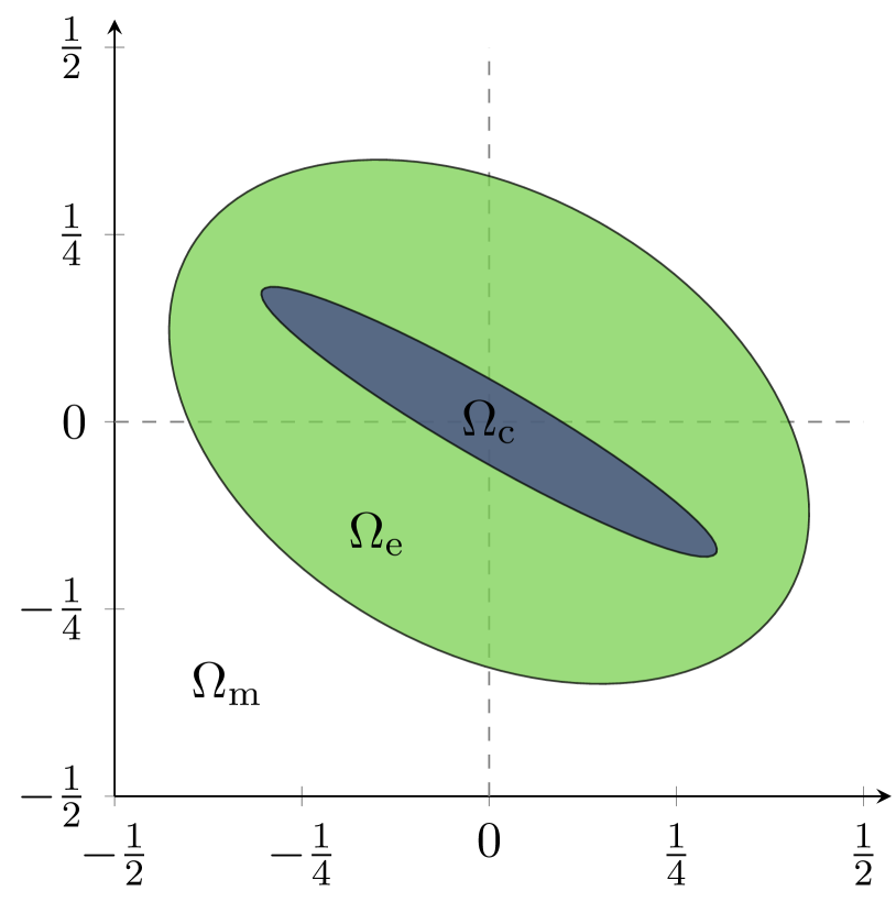
A prototypical structure that is introduced in [3] is the generalized Hashin structure, a geometry that is based on publications of Milton, see [16]. It consists of two confocal ellipses embedded in a surrounding material, see Figure 3. The centre () and coating () ellipses have isotropic behaviour and the matrix material () is built in such a way that it is unaffected by the inclusion for a chosen macroscopic strain . For this special kind of structure analytic expressions for the strain field and the action of the effective matrix are known.
In the following we take exactly the same parameters as in [3], i.e. for the ellipses with parametrization
and we choose , and for the inner and outer ellipsis and , respectively. The structure is then rotated by . For the inner and outer ellipsis we choose isotropic material laws with Poisson’s ratio in both ellipses and the matrix material and Young’s moduli and for the inner and outer ellipsis, respectively. The material law for the surrounding matrix material can then be determined by the formulae in [3, Section 4.2].
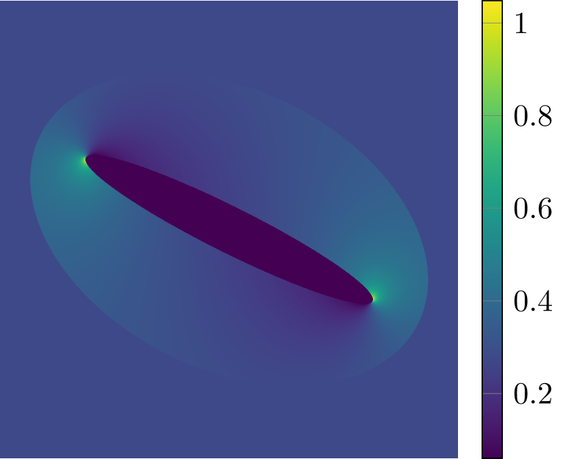
A solution for the first component of the strain field is depicted in Figure 3 and taken for instructional purposes directly from [3].
All numerical results in this section were obtained by solving (20) with a fixed-point iteration on as described in [19] up to an relative error of using a Cauchy criterion.
4.1 De la Vallée Poussin means
In [3] the authors study the influence of the pattern matrix on the solution field and the quality of the effective matrix . We take the following pattern matrices:
They correspond to a tensor product grid (), a tensor product grid rotated by () and the minimal -error () achieved. The matrices and have a determinant of whereas the so-called quincux pattern has sampling points.
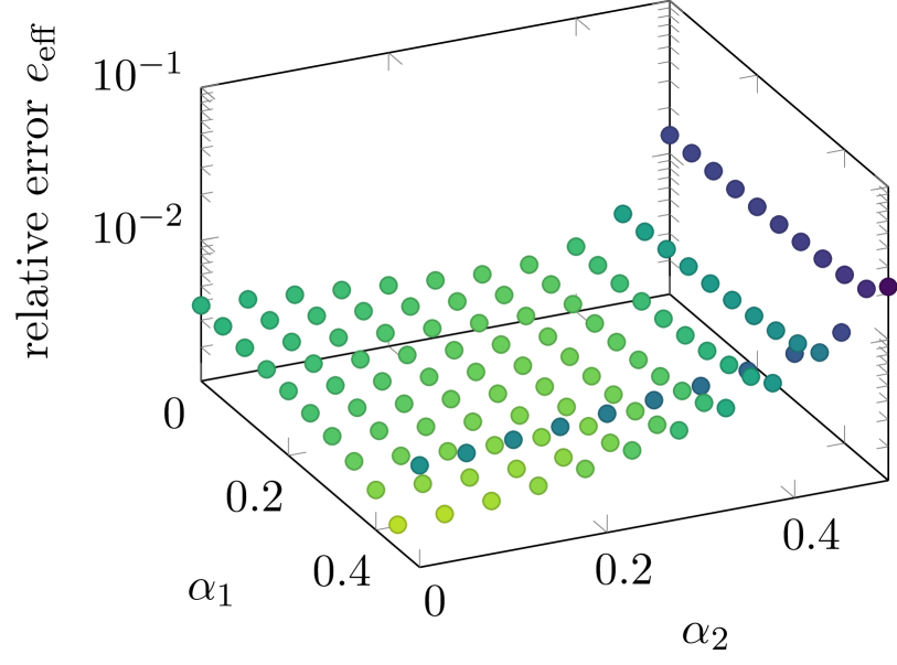
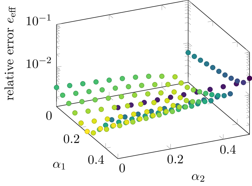
First we study how using de la Vallée Poussin means changes the quality of the effective stiffness matrix and the strain field. The Box splines used in frequency domain to define the means allow to use different slopes in each direction of the de la Vallée Poussin mean and thus one can expect to reduce the Gibbs phenomenon in different directions. For the following study the functions are parametrized with and for .
The parameters and correspond to damping the Fourier coefficients of the de la Vallée Poussin mean along the directions and , respectively. In the space domain they introduce a better localization [11] along and , respectively.
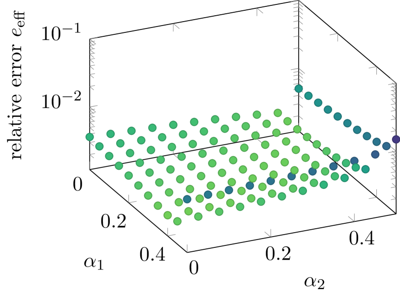
The result of these experiments regarding the effective stiffness matrix is shown in Figure 4. The relative effective error
is depicted with from (20). Parameters correspond to the modified Dirichlet kernel and correspond to the Fejér kernel .
For , the error in the effective stiffness matrix changes from for the modified Dirichlet kernel to the optimum at and with . For it changes from to for and . The solution for can be improved upon by de la Vallée Poussin means with and which results in of the Fourier approach on patterns being reduced to . When approaching either or the value of drastically increases. The errors for the solution using the Dirichlet kernel and the modified Dirichlet kernel, i.e. for , are almost the same and thus not marked in the plots above.
The study in [3] suggests that by changing the pattern one can improve the quality of the solution and the effective stiffness matrix. The experiments from above show that one can improve these results even further by extending the theory to translation invariant spaces. Especially for the tensor product grid, i.e. for data given on a regular voxel grid like for example from a computer tomography image, a suitable choice of the space of translates could here reduce the error in the effective stiffness by .
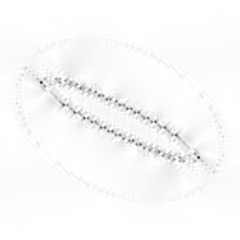
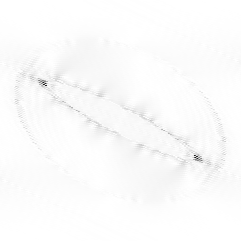
Figure 5 shows the logarithmic error of the analytic solution to solution , i.e. . The top row shows the error corresponding to the de la Vallée Poussin means with parameters and which give the smallest . The middle row shows the error using the Dirichlet kernel. For illustration purposes each pixel has the form of the corresponding unit cell centred at each pattern point .
The value of the relative -error is given by the formula
While the error in the effective stiffness matrix can be drastically improved using de la Vallée Poussin means, the -error gets larger, however, only be a few percent. The strain field stemming from the numerical computation using de la Vallée Poussin means shows less Gibbs phenomena as can be seen most prominently in the solution for pattern matrix .
The decrease of is caused by the smoothing of the Gibbs phenomena around discontinuities of the solution with higher . With smaller de la Vallée Poussin parameters and the polynomial reproduction is better and thus interfaces (edges) are sharper. In total they introduce a trade off between damping Gibbs phenomena and sharpness of the interfaces.

| , | , |
|---|---|
| , | |
| . |
| , | , |
|---|---|
| , | |
| . |
| , | , |
|---|---|
| , | |
| . |
| , | , |
|---|---|
| . |
| , | , |
|---|---|
| . |
| , | , |
|---|---|
| . |
| , | , |
|---|---|
| . |
| , | , |
|---|---|
| . |
| , | , |
|---|---|
| . |
4.2 Periodised Box Splines
Finite elements with one quadrature point are directly included in this framework. They are obtained by choosing a suitable Box spline as ansatz function for the space of translates . In the bottom row of Figure 5 the logarithmic error between the numerical solution and the analytical solution is depicted, using the matrices , , from above. For all computations the Box spline with
| (23) |
is used. This ansatz function corresponds to a finite element of third order with reduced integration. The bracket sums in (14) are precomputed with terms each.
A comparison of the relative error in the effective matrix between the Box splines (bottom row) and the Dirichlet kernel (middle row) shows that for matrices and the error in the effective matrix can be reduced by about , whereas the error is approximately tripled for . The -error is increased in all three cases. The pattern matrix was optimized for the Dirichlet kernel with respect to the -norm. For Box splines this pattern leads to an aliasing effect reducing the quality of the solution.
The choice of the Box spline was not optimized and the quality of the effective matrix might be further increased by a different choice of . This corresponds to a fine tuning with respect to dominant directions in the pattern unit cell .
5 Conclusion
The introduced framework unifies and analyses for the first time the truncated Fourier series approach and finite element ansatz functions. In this framework the periodised Green operator possesses the same properties as the Green operator of the Galerkin method of Vondřejc et.al [27]. The projection operator emerges as a special case of Dirichlet kernel translates. The periodised Green operator can further be characterised to be a projection if and only if the space is the one derived from a Dirichlet kernel. The finite element method emerges for certain Box splines and thus the constant finite elements of Brisard and Dormieux [8] are included. For these Box splines the infinite Bracket sums have to be precomputed up to a given precision, but the algorithm has the same complexity as the Fourier framework.
Finite elements with more sophisticated quadrature rules can also be viewed in terms of this framework. However, their performance is an open question for future work. How to choose a certain Box spline especially with respect to anisotropies present in the data is a point for further analysis. Convergence of the numerical discretisation towards the continuous case and the convergence of the algorithm will be dealt with in a paper on our road map. Both seem to be strongly suggested by the numerical results. Finally the periodic multiresolution analysis can be used to extend this framework in order to exploit sparsity properties of given data. This is also a point for future work.
Acknowledgement
The authors would like to thank Bernd Simeon and Gabriele Steidl for their valuable comments on preliminary versions of this manuscript and fruitful discussions.
References
- [1] Ronny Bergmann “The fast Fourier transform and fast wavelet transform for patterns on the torus” In Appl. Comp. Harmon. Anal. 35.1, 2013, pp. 39–51 DOI: 10.1016/j.acha.2012.07.007
- [2] Ronny Bergmann “Translationsinvariante Räume multivariater anisotroper Funktionen auf dem Torus”, 2013 URL: http://www.math.uni-luebeck.de/mitarbeiter/bergmann/publications/diss\_bergmann.pdf
- [3] Ronny Bergmann and Dennis Merkert “A Framework for FFT-based Homogenization on Anisotropic Lattices”, 2016 arXiv:1605.05712
- [4] Ronny Bergmann and Jürgen Prestin “Multivariate Anisotropic Interpolation on the Torus” In Approximation Theory XIV: San Antonio 2013 Cham: Springer International Publishing, 2014, pp. 27–44 DOI: 10.1007/978-3-319-06404-8˙3
- [5] Ronny Bergmann and Jürgen Prestin “Multivariate Periodic Wavelets of de la Vallée Poussin Type” In J. Fourier. Anal. Appl. 21.2, 2014, pp. 342–369 DOI: 10.1007/978-3-319-06404-8˙3
- [6] Carl Boor, Klaus Höllig and Sherman Riemenschneider “Box Splines” New York: Springer-Verlag, 1993 DOI: 10.1007/978-1-4757-2244-4
- [7] Carl Boor, Klaus Höllig and Sherman D Riemenschneider “Bivariate cardinal interpolation by splines on a three-direction mesh” In Illinois J. Math. 29.4, 1985, pp. 533–566
- [8] S Brisard and L Dormieux “FFT-based methods for the mechanics of composites: A general variational framework” In Comput. Mater. Sci. 49.3, 2010, pp. 663–671 DOI: 10.1016/j.commatsci.2010.06.009
- [9] Sébastien Brisard and Luc Dormieux “Combining Galerkin approximation techniques with the principle of Hashin and Shtrikman to derive a new FFT-based numerical method for the homogenization of composites” In Comput. Method. Appl. M. 217 Elsevier, 2012, pp. 197–212 DOI: 10.1016/j.cma.2012.01.003
- [10] Charles K Chui and Chun Li “A general framework of multivariate wavelets with duals” In Appl. Comp. Harmon. Anal. 1.4, 1994, pp. 368–390 DOI: 10.1006/acha.1994.1023
- [11] Say Song Goh and Tim NT Goodman “Uncertainty principles and asymptotic behavior” In Appl. Comp. Harmon. Anal. 16.1 Elsevier, 2004, pp. 19–43 DOI: 10.1016/j.acha.2003.10.001
- [12] Matthias Kabel, Dennis Merkert and Matti Schneider “Use of composite voxels in FFT-based homogenization” In Comput. Method. Appl. M. 294, 2015, pp. 168–188 DOI: 10.1016/j.cma.2015.06.003
- [13] Lutz Kämmerer, Daniel Potts and Toni Volkmer “Approximation of multivariate periodic functions by trigonometric polynomials based on rank-1 lattice sampling” In J. Complexity 31, 2015, pp. 543–576 DOI: 10.1016/j.jco.2015.02.004
- [14] Dirk Langemann and Jürgen Prestin “Multivariate periodic wavelet analysis” In Appl. Comp. Harmon. Anal. 28.1, 2010, pp. 46–66 DOI: 10.1016/j.acha.2009.07.001
- [15] JC Michel, H Moulinec and P Suquet “A computational method based on augmented Lagrangians and fast Fourier transforms for composites with high contrast” In Comput. Model. Eng. Sci. 1.2, 2000, pp. 79–88 DOI: 10.3970/cmes.2000.001.239
- [16] G. W. Milton “The theory of composites” Cambridge University Press, 2002 DOI: 10.1017/CBO9780511613357
- [17] Nachiketa Mishra, Jaroslav Vondřejc and Jan Zeman “A comparative study on low-memory iterative solvers for FFT-based homogenization of periodic media” In J. Comput. Phys. 321 Elsevier, 2016, pp. 151–168 DOI: 10.1016/j.jcp.2016.05.041
- [18] H. Moulinec and P. Suquet “A fast numerical method for computing the linear and nonlinear mechanical properties of composites” In C. R. Acad. Sci. II B 318.11, 1994, pp. 1417–1423
- [19] H. Moulinec and P. Suquet “A numerical method for computing the overall response of nonlinear composites with complex microstructure” In Comput. Method. Appl. M. 157.1-2, 1998, pp. 69–94 DOI: 10.1016/s0045-7825(97)00218-1
- [20] Gisela Pöplau “Multivariate periodische Interpolation durch Translate und deren Anwendung”, 1995
- [21] Jürgen Prestin and Kathi Selig “Interpolatory and orthonormal trigonometric wavelets” In Signal and Image Representation in Combined Spaces 7, Wavelet Analysis and Its Applications Academic Press, 1998, pp. 201–255 DOI: 10.1016/S1874-608X(98)80009-5
- [22] Matti Schneider, Dennis Merkert and Matthias Kabel “FFT-based homogenization for microstructures discretized by linear hexahedral elements” In Int. J. Numer. Meth. Eng. Wiley Online Library, 2016 DOI: 10.1002/nme.5336
- [23] Matti Schneider, Felix Ospald and Matthias Kabel “Computational homogenization of elasticity on a staggered grid” In Int. J. Numer. Meth. Eng. Wiley Online Library, 2015 DOI: 10.1002/nme.5008
- [24] K. Selig “Periodische Wavelet-Packets und eine gradoptimale Schauderbasis”, 1998
- [25] Frauke Sprengel “Interpolation und Waveletzerlegung multivariater periodischer Funktionen”, 1997
- [26] Thu-Huong Tran, Vincent Monchiet and Guy Bonnet “A micromechanics-based approach for the derivation of constitutive elastic coefficients of strain-gradient media” In Int. J. Solids. Struct. 49.5 Elsevier, 2012, pp. 783–792 DOI: 10.1016/j.ijsolstr.2011.11.017
- [27] Jaroslav Vondřejc, Jan Zeman and Ivo Marek “An FFT-based Galerkin method for homogenization of periodic media” In Comput. Math. Appl. 68.3 Elsevier, 2014, pp. 156–173 DOI: 10.1016/j.camwa.2014.05.014
- [28] François Willot “Fourier-based schemes for computing the mechanical response of composites with accurate local fields” In C. R. Mécanique 343.3 Elsevier, 2015, pp. 232–245 DOI: 10.1016/j.crme.2014.12.005
- [29] Jan Zeman, Jaroslav Vondřejc, Jan Novák and Ivo Marek “Accelerating a FFT-based solver for numerical homogenization of periodic media by conjugate gradients” In J. Comput. Phys. 229.21, 2010, pp. 8065–8071 DOI: 10.1016/j.jcp.2010.07.010