Displacement Convexity in Spatially
Coupled Scalar Recursions

Abstract

We introduce a technique for the analysis of general spatially coupled systems that are governed by scalar recursions. Such systems can be expressed in variational form in terms of a potential functional. We show, under mild conditions, that the potential functional is displacement convex and that the minimizers are given by the fixed points of the recursions. Furthermore, we give the conditions on the system such that the minimizing fixed point is unique up to translation along the spatial direction. The condition matches those in [1] for the existence of spatial fixed points. Displacement convexity applies to a wide range of spatially coupled recursions appearing in coding theory, compressive sensing, random constraint satisfaction problems, as well as statistical mechanical models. We illustrate it with applications to Low-Density Parity-Check and generalized LDPC codes used for transmission on the binary erasure channel, or general binary memoryless symmetric channels within the Gaussian reciprocal channel approximation, as well as compressive sensing.

I Introduction

Spatially coupled systems have been used recently in various frameworks such as coding [2], [3], [4], [5] (for a review of applications in the context of communications see [5] and references therein), compressive sensing [6], [7], statistical physics [8], [9], and random constraint satisfaction problems [10], [11]. These systems exhibit excellent performance, often optimal, under low complexity message passing algorithms, due to the threshold saturation phenomenon [5], [12], [13]. For example, spatially coupled high-degree regular LDPC codes achieve the Shannon capacity under belief propagation [5], [13]. Another line of research has used spatially coupled constructions to prove results about the original uncoupled underlying model. For example, this idea was used to obtain proofs of replica-symmetric formulas for the mutual information in coding [14], in rank-one matrix factorization [15], and to improve provable algorithmic lower bounds on phase transition thresholds of random constraint satisfaction problems [11].

Given the success of spatial coupling in a wide variety of problems, it should hardly come as a surprise that there are fundamental mathematical structures behind spatially coupling. This paper is concerned with a somewhat hidden convexity structure called displacement convexity. Some of our preliminary work on this matter appeared in [16], [17], [18].

The large system asymptotic performance of spatially coupled systems is assessed by the solutions of coupled density evolution (DE) type update equations. In general, the fixed points of these equations can be viewed as the stationary point equations of a functional that is typically called the “potential functional” and is an “average form” of the Bethe free energy [19] of the underlying graphical model. It has already been recognized that this variational formulation is a powerful tool to analyze DE updates under suitable initial conditions [1], [8], [12], [13]. There are various possible formulations of this potential functional; in this paper, we will use the representation from [1] for scalar systems.

In a previous contribution [16], we showed that the potential, in the form given in [12], associated to a spatially coupled low-density parity-check (LDPC) code whose single system is the $(\ell,r)$-regular Gallager ensemble, with transmission over the binary erasure channel with parameter $\epsilon$, or the BEC($\epsilon$), has a convex structure called displacement convexity. This structure is well-known in the theory of optimal transport [21]. In fact, the potential we consider in [16] is not convex in the usual sense but it is in the sense of displacement convexity. This, in itself, is an interesting property. Although the formalism in [16] can be extended to more general scalar recursions, for example, those pertaining to irregular LDPC codes, it does not appear to extend to a very wide class of general scalar recursions. The main purpose of the present paper is to prove that a rather general class of scalar systems also exhibits the property of displacement convexity, and even strict displacement convexity under rather mild assumptions. Although the analysis of the present paper is similar in spirit to [16] it is also significantly different and more far reaching in its range of applications. We use the potential in the representation of [1] which allows to obtain much more general proofs that hold under quite mild conditions. The results are applicable to recursions appearing not only in coding, but also in compressive sensing and random constraint satisfaction problems.

The main propositions of this paper are: Proposition V.1 that states that the potential functional has the displacement convexity property; Proposition VI.1 that asserts that monotonic minimizers of the potential functional are fixed point solutions of the spatially coupled DE equations (in a generalized sense); Proposition VII.4 that gives the condition for the unicity of the minimizers up to translations along the spatial axis. It is also of interest that the potential functional satisfies a rearrangement inequality, namely Proposition III.4 that ensures that one can find minimizers among monotonic spatial fixed points. The conditions for our results to hold are rather mild and essentially match those in [1] for the existence of spatial fixed points.

This manuscript is organized as follows. Section II introduces spatially coupled recursions and the variational formulation. In Section III, we prove rearrangement inequalities that allow us to reduce the search for minima of the potential to a space of monotonic functions, and, in Section IV, we discuss the existence question using the direct method from functional analysis. The potential is shown to be displacement convex in Section V. In Section VI, we generalize the notion of fixed point solutions to the DE equations and show that such generalized solutions are minimizers of the potential. Unicity of the minimizer is addressed in Section VII. In Section VIII, we illustrate displacement convexity with applications to coding and compressive sensing.

II Set Up and Variational Formulation

In this section, we explain the set-up for general spatially coupled scalar recursions and give a variational formulation of these recursions. The fixed point equations of the scalar recursions will be generically called “density evolution” (DE) equations. The case of regular $(\ell,r)$-LDPC code ensembles with transmission over the BEC$(\epsilon)$ will serve as a concrete running example for the setting.

Consider the pair of DE fixed point equations

$$\begin{cases}u=h_{g}(v),\\ v=h_{f}(u),\end{cases}$$ (1)

where $u,v\in[0,1]$. The update functions $h_{f}$, $h_{g}$ are assumed to be non-decreasing from $[0,1]$ to $[0,1]$, and normalized such that $h_{f}(0)=h_{g}(0)=0$ and $h_{f}(1)=h_{g}(1)=1$. We will think of them as EXIT-like curves of DE $(u,h_{f}(u))$ and $(h_{g}(v),v)$ for $u,v\in[0,1]$ (see Fig. 1). It is always possible to adopt this normalization in specific applications.

• Take an $(\ell,r)$-regular Gallager ensemble, with transmission over the BEC($\epsilon$). Let $\mathtt{y}$ (resp. $\mathtt{x}$) be the erasure probability emitted by the check (resp. variable) nodes. The DE fixed point equations are $\mathtt{y}=1-(1-\mathtt{x})^{r-1}$ and $\mathtt{x}=\epsilon\mathtt{y}^{\ell-1}$. In this paper, we are interested in the specific value $\epsilon=\epsilon_{\text{\tiny MAP}}$ which is the MAP threshold of the ensemble. Let $\mathtt{x}_{\text{\tiny MAP}}$, $\mathtt{y}_{\text{\tiny MAP}}$ be the non-trivial stable fixed point when $\epsilon=\epsilon_{\text{\tiny MAP}}$. To achieve the normalization of (1) we make the change of variables $\mathtt{y}=\mathtt{y}_{\text{\tiny MAP}}u$ and $\mathtt{x}=\mathtt{x}_{\text{\tiny MAP}}v$, so that the DE equations become $u=\mathtt{y}_{\text{\tiny MAP}}^{-1}(1-(1-\mathtt{x}_{\text{\tiny MAP}}v)^{r-1})$ and $v=\epsilon_{\text{\tiny MAP}}\mathtt{x}_{\text{\tiny MAP}}^{-1}\mathtt{y}_{\text{\tiny MAP}}^{\ell-1}u^{\ell-1}$. Note that we must have $1=\mathtt{y}_{\text{\tiny MAP}}^{-1}(1-(1-\mathtt{x}_{\text{\tiny MAP}})^{r-1})$ and $1=\epsilon_{\text{\tiny MAP}}\mathtt{x}_{\text{\tiny MAP}}^{-1}\mathtt{y}_{\text{\tiny MAP}}^{\ell-1}$. We then set

  $$\begin{cases}h_{g}(v)=\mathtt{y}_{\text{\tiny MAP}}^{-1}(1-(1-\mathtt{x}_{\text{\tiny MAP}}v)^{r-1}),\\ h_{f}(u)=u^{\ell-1},\end{cases}$$ (2)

  which satisfy the required normalizations $h_{f}(0)=h_{g}(0)=0$ and $h_{f}(1)=h_{g}(1)=1$. The corresponding EXIT curves have three intersections. The one at $(0,0)$ corresponds to the trivial fixed point of DE, the one at $(1,1)$ corresponds to the stable non-trivial fixed point of DE, and the third one at a middle point corresponds to the unstable fixed point.

The natural setting for displacement convexity, at least in the context of spatial coupling, is the continuum setting, which can be thought of as an approximation of the corresponding discrete system in the regime of large spatial length and coupling window size. The continuum limit has already been introduced in the literature as a convenient means to analyze the behavior of an originally discrete model [1], [6], [8].

Consider a spatially coupled system with an averaging window $w:\mathds{R}\to\mathds{R}$ which is always assumed to be bounded, non-negative, even, integrable, and normalized such that $\int_{\mathds{R}}{\mathrm{d}}x\,w(x)=1.$ The averaging window is the means for the “coupling” in “spatial coupling”. Let us define the constant

$$C_{w}:=\int_{\mathds{R}}{\mathrm{d}}x\,|x|w(x).$$ (3)

We assume throughout the paper that $C_{w}$ is finite. As we shall see, this is directly related to finiteness of the potential. Let $f,g:\mathds{R}\to[0,1]$ be two functions and denote by $f^{w}=f\otimes w$ and $g^{w}=g\otimes w$ their usual convolutions with $w$, i.e., $f^{w}(x)=\int_{\mathds{R}}{\mathrm{d}}x\,f(y)w(x-y)$ and $g^{w}(x)=\int_{\mathds{R}}{\mathrm{d}}x\,g(y)w(x-y)$. The pair of fixed point DE equations of a spatially coupled scalar continuous system are

$$\begin{cases}g(x)=h_{g}(f^{w}(x)),\\ f(x)=h_{f}(g^{w}(x)),\end{cases}$$ (4)

where $x\in\mathds{R}$ is the spatial position. We will often refer to the functions $f$, $g$ as profiles and to $h_{f}$, $h_{g}$ as update functions. A pair of profiles $f,g:\mathds{R}\to[0,1]$ that solves the above equations almost everywhere will be called a fixed point, FP for short. Note that (4) are non-local equations because of the coupling through $w.$

In this paper, we are interested in profiles $p:\mathds{R}\rightarrow[0,1]$ ($p$ denotes a generic profile like $f$ and $g$) that satisfy the limit conditions

$$\lim\limits_{x\rightarrow-\infty}p(x)=0,\qquad\lim\limits_{x\rightarrow+\infty}p(x)=1.$$ (5)

We note that these two limit values are the extreme fixed points of (1) We will refer to such profiles as interpolating profiles. A pair $f,g$ of interpolating profiles that solves (4) is called an interpolating FP.

• A function $p:\mathds{R}\rightarrow[0,1]$ satisfying (5) is called an interpolating profile. A pair $f,g$ of interpolating profiles that solves (4) almost everywhere, i.e., up to a set of measure zero, is called an interpolating fixed point (FP).

In Section III, we show that when minimizing the potential functional over the space of interpolating profiles we can focus on monotonic (non-decreasing) profiles.

Figure 1: A generic example of the systems we consider. The EXIT-like curves are $h_{f}$ (in red) and $h_{g}^{-1}$ (in blue). The signed area $A(h_{f},h_{g};1)$ from (7) is the sum of the light gray areas (positively signed) and the dark gray areas (negatively signed), and it is equal to $0$.

II-A Potential function associated to (1)

In [1] the following potential function is introduced,

$$\phi(h_{f},h_{g};u,v)=\int_{0}^{u}\text{d}u^{\prime}\,h_{g}^{-1}(u^{\prime})+\int_{0}^{v}\text{d}v^{\prime}\,h_{f}^{-1}(v^{\prime})\,-uv\,.$$ (6)

Often, when they are clear from context or irrelevant, we will drop the update functions $h_{f}$ and $h_{g}$ as arguments from the notation and denote this potential function by $\phi(u,v)$. Since $h_{g}^{-1}$ and $h_{f}^{-1}$ are non-decreasing the potential $\phi(u,v)$ is convex in $u$ for fixed $v$ and convex in $v$ for fixed $u.$ It is minimized over $v$ by setting $v=h_{f}(u)$ and over $u$ by setting $u=h_{g}(v)$.

Substituting $v=h_{f}(u)$ in (6), we obtain the integral of the signed area between the two EXIT curves (see fig. 1) as

$$A(h_{f},h_{g};u) =\phi(h_{f},h_{g};u,h_{f}(u))$$

$$=\int_{0}^{u}\mathrm{d}u^{\prime}\,(h_{g}^{-1}(u^{\prime})-h_{f}(u^{\prime})).$$ (7)

Note that this is the signed area bounded by the two curves and the region between the vertical axis at the origin and a vertical axis at $u$.

In [1], the following key result was shown. It states that for an interpolating FP to exist the potential $\phi$ must be minimal at both limit points.

Lemma II.1

If there exists an interpolating FP solution to (4), then $\phi(h_{f},h_{g};u,v)\geq 0$ for all $u,v\in[0,1]$ and $A(h_{f},h_{g};1)=\phi(h_{f},h_{g};1,1)=0.$

The result applies not only to interpolating FPs but also to a relaxed definition of interpolating “consistent” FPs (CFPs) that we define in Section VI. In [1], when the assumption $\phi(h_{f},h_{g};1,1)=0$ is made, the condition $\phi(h_{f},h_{g};u,v)\geq 0$ for all $u,v\in[0,1]$ is termed the positive gap condition (PGC). In this paper we will additionally assume $\phi(h_{f},h_{g};1,1)=0$ throughout so the term positive gap condition will be used to imply both this equality and the inequality in Lemma II.1.

When the inequality in Lemma II.1 is strict, i.e., $\phi(h_{f},h_{g};u,v)>0$ for $(u,v)\not\in\{(0,0),(1,1)\}$ then the condition is termed the strictly positive gap condition (SPGC) in [1]. In this case, it was shown that an interpolating fixed point profile exists provided $w$ is strictly positive on the interior of some interval $[-W,W]$ and zero off of the interval. This support condition on $w$ can be relaxed under various other conditions (see [1]).

• We say that the positive gap condition (PGC) is satisfied when $\phi(h_{f},h_{g};1,1)=0$ and $\phi(h_{f},h_{g};u,v)\geq 0$ for all $u,v\in[0,1]$. The strictly positive gap condition is satisfied when $\phi(h_{f},h_{g};1,1)=0$ and $\phi(h_{f},h_{g};u,v)>0$ for $(u,v)\not\in\{(0,0),(1,1)\}$.

• For the $(\ell,r)$-regular Gallager ensemble, with transmission over the BEC($\epsilon$) with $\epsilon=\epsilon_{\rm MAP}$ we have the potential function

  $$\phi(u,v)= \frac{1}{\mathtt{x}_{\text{\tiny MAP}}}\Big{\{}u-\frac{r-1}{\mathtt{y}_{\text{\tiny MAP}}r}(1-(1-\mathtt{y}_{\text{\tiny MAP}}u)^{\frac{r}{r-1}}))\Big{\}}+\frac{\ell-1}{\ell}v^{\frac{\ell}{\ell-1}}-uv,$$

  and the signed area

  $$A(h_{f},h_{g};u)= \frac{1}{\mathtt{x}_{\text{\tiny MAP}}}\Big{\{}u+\frac{r-1}{\mathtt{y}_{\text{\tiny MAP}}r}((1-\mathtt{y}_{\text{\tiny MAP}}u)^{\frac{r}{r-1}}-1)\Big{\}}-\frac{u^{\ell}}{\ell}.$$

  Moreover, we have $A(h_{f},h_{g};1)=0$. In fact, this last constraint together with the two fixed point equations $\mathtt{y}_{\text{\tiny MAP}}=1-(1-\mathtt{x}_{\text{\tiny MAP}})^{r-1}$ and $\mathtt{x}_{\text{\tiny MAP}}=\epsilon_{\text{\tiny MAP}}\mathtt{y}_{\text{\tiny MAP}}^{\ell-1}$ completely determine $\epsilon_{\text{\tiny MAP}}$, $\mathtt{x}_{\text{\tiny MAP}}$ and $\mathtt{y}_{\text{\tiny MAP}}$. The SPGC holds for this example (see Section VIII for further illustration).

II-B Potential functional of the spatially coupled system (4)

The solutions of spatially coupled DE equations (4) are given by the stationary point of a potential functional $\mathcal{W}$ of $f$ and $g$ defined below. This can be checked by setting the functional derivatives of this potential functional with respect to each of $f$ and $g$ to zero. We set

$$\mathcal{W}(f,g)=\int_{\mathds{R}}\mathrm{d}x\,I_{f,g,w}(x),$$ (8)

where we have introduced the notation

$$I_{f,g,w}(x)= \int_{0}^{g(x)}\mathrm{d}u\,h_{g}^{-1}(u)+\int_{0}^{f(x)}\mathrm{d}v\,h_{f}^{-1}(v)-f^{w}(x)g(x).$$ (9)

• For the $(\ell,r)$-regular LDPC code and transmission over the BEC($\epsilon$), the potential (8) is

  $$\mathcal{W} (f,g)=\int\limits_{\mathds{R}}\mathrm{d}x\,\Big{[}\frac{1}{\mathtt{x}_{\text{\tiny MAP}}}\big{\{}g(x)-\frac{r-1}{\mathtt{y}_{\text{\tiny MAP}}r}(1-(1-\mathtt{y}_{\text{\tiny MAP}}g(x))^{\frac{r}{r-1}})\big{\}}+\frac{\ell-1}{\ell}f(x)^{\frac{\ell}{\ell-1}}-f^{w}(x)g(x)\Big{]}.$$

Note that the limit of the integrand in (8) (and the example) vanishes when $x\to-\infty$ because of the condition (5) on the profiles. It also vanishes when $x\to+\infty$ because of (5) and $A(h_{f},h_{g};1)=0$. However, this does not suffice for the existence of the integral, essentially due to the fact that $f^{w}-f$ may not be Lebesgue integrable (for monotonic profiles this difficulty does not arise). So it is possible that ${\cal W}(f,g)$ fails to be well-defined as a Lebesgue integral for some choices of the interpolating profiles.

Once we consider interpolating profiles and assume the PGC and that $C_{w}<\infty$, we can circumvent this technical issue by defining the potential functional as

$${\cal W}(f,g)=\lim_{A,B\rightarrow\infty}\int_{-A}^{B}{\mathrm{d}}xI_{f,g,w}(x).$$ (10)

We show below that the limit always exists (it is possibly $+\infty$).

Lemma II.2

Assuming the PGC, we have for any interpolating profile pair $f,g$ that

$${\cal W}(f,g)\geq\int_{\mathds{R}}{\mathrm{d}}x\,\phi(f^{w}(x),g(x)),$$ (11)

and given a sequence of interpolating pairs $f_{i},g_{i}$ converging pointwise almost everywhere to an interpolating pair $f,g$ we have

$$\liminf_{i\rightarrow\infty}{\cal W}(f_{i},g_{i})\geq{\cal W}(f,g).$$ (12)

Proof:

Define $H_{f}(f)=\int_{0}^{f}{\mathrm{d}}v\,h_{f}^{-1}(v)$ and $H_{g}(g)=\int_{0}^{g}{\mathrm{d}}u\,h_{g}^{-1}(u)$. Note that

$$I_{f,g,w}=(H_{g}\circ g)+(H_{f}\circ f)-f^{w}g.$$

Now, if we define

$$\tilde{I}_{f,g,w}=(H_{g}\circ g)+(H_{f}\circ f)^{w}-f^{w}g,$$

then

$$\int_{-A}^{B}{\mathrm{d}}x\,I_{f,g,w}(x) =\int_{-A}^{B}{\mathrm{d}}x\,\tilde{I}_{f,g,w}(x)+\int_{-A}^{B}{\mathrm{d}}x\,(I_{f,g,w}(x)-\tilde{I}_{f,g,w}(x))$$

$$=\int_{-A}^{B}{\mathrm{d}}x\,\tilde{I}_{f,g,w}(x)+\int_{-A}^{B}{\mathrm{d}}x((H_{f}\circ f)-(H_{f}\circ f)^{w}(x)).$$

Taking limits $A,B\to+\infty$ by definition (10) and Lemma .1, we obtain

$${\cal W}(f,g)=\lim_{A,B\to+\infty}\int_{-A}^{B}{\mathrm{d}}x\,\tilde{I}_{f,g,w}(x).$$

We will shortly see that the PGC implies $\tilde{I}_{f,g,w}(x)$ is non-negative so that ${\cal W}(f,g)$ is well defined (it is possibly $+\infty$). This also means that it is possible to adopt

$${\cal W}(f,g)=\int_{\mathds{R}}{\mathrm{d}}x\,\tilde{I}_{f,g,w}(x),$$ (13)

as an alternative expression for ${\cal W}(f,g)$.

Now, note that $H_{f}(f)$ and $H_{g}(g)$ are convex functions because $h_{f}^{-1}$ and $h_{g}^{-1}$ are non-decreasing. Indeed

$$H_{f}(f+a)-H_{f}(f) =\int_{f}^{f+a}{\mathrm{d}}v\,h_{f}^{-1}(v)\geq ah_{f}^{-1}(f)=aH_{f}^{\prime}(f).$$

By Jensen’s inequality we have

$$(H_{f}\circ f)^{w}\geq(H_{f}\circ f^{w}),$$

and we therefore obtain

$$\tilde{I}_{f,g,w}(x)\geq\phi(f^{w}(x),g(x)),$$ (14)

which proves the non-negativity of $\tilde{I}_{f,g,w}(x)$ since $\phi(f^{w}(x),g(x))$ is non-negative by the PGC.

Integrating (14) and using (13), we obtain the first claim (11) of the lemma. Furthermore, we get the second claim (12) directly by applying Fatou’s lemma to (13) (we can apply Fatou’s lemma since by (14) $\tilde{I}_{f_{i},g_{i},w}$ is a non-negative sequence, and it converges to $\tilde{I}_{f,g,w}$). ∎

Let us remark that in the process of proving this lemma, we have seen $\mathcal{W}(f,g)$ can be defined as (10) or equivalently as (13), as long as we assume the PGC, interpolating profiles and $C_{w}<+\infty$.

II-C Discussion

In Section VI, we show that among all interpolating profiles, monotonic interpolating CFPs yield minimizers of $\mathcal{W}$. To do that, we use rearrangement properties that are summarized in Section III. For a fixed $f$, we always have $\mathcal{W}(f,g)\geq\mathcal{W}(f,h_{g}\circ f^{w})$. This is because $I_{f,g,\omega}(x)$ is convex in $g(x)$ for fixed $f(x)$ and setting $g(x)=h_{g}(f^{w}(x))$ minimizes $I_{f,g,\omega}(x)$ over $g(x)$ for fixed $f(x)$.

One of the main results of this paper is to show the displacement convexity of $\mathcal{W}$ in its two arguments. More precisely, we can think of interpolating between two pairs $(f_{0},g_{0})$ and $(f_{1},g_{1})$ of monotonic profiles by interpolating their inverse functions. Hence, we consider

$$\begin{cases}f_{\lambda}^{-1}&=(1-\lambda)f_{0}^{-1}+\lambda f_{1}^{-1},\\ g_{\lambda}^{-1}&=(1-\lambda)g_{0}^{-1}+\lambda g_{1}^{-1},\end{cases}$$

and show that $\mathcal{W}(f_{\lambda},g_{\lambda})$ is a convex function of $\lambda.$ Note that for a monotonic interpolating profile $p$ the inverse function $p^{-1}(u)$ is uniquely defined for almost all $u\in(0,1)$ and right and left limits $p^{-1}(u+)$ and $p^{-1}(u-)$, respectively, are uniquely determined. Displacement convexity is explained in more detail in Section V.

Displacement convexity applies only to monotonic profiles. In the next section, we address the conditions under which one can conclude that minimizers of $\mathcal{W}$ satisfying (5) can taken to be monotonic.

The following quantities will play a crucial role in the remainder of this work,

$$\Omega(x)=\int_{-\infty}^{x}\mathrm{d}z\,w(z),\qquad V(x)=\int_{-\infty}^{x}\mathrm{d}z\,\Omega(z).$$ (15)

Here, $V$ is called the kernel for reasons that will become clear. As will be seen, displacement convexity arises from the convexity of $V$.

Lemma II.3

Assume that $C_{w}<\infty$. Then, $V$ is well defined and convex.

Proof:

Using integration by parts, we can write

$$V(x)=\int_{-\infty}^{x}\mathrm{d}z\,\Omega(z)=x\,\Omega(x)\Big{|}_{-\infty}^{x}-\int_{-\infty}^{x}\mathrm{d}z\,zw(z).$$ (16)

For $z\leq 0$, we have

$$\int_{-\infty}^{z}\mathrm{d}x\,|x|w(x)\geq\int_{-\infty}^{z}\mathrm{d}x\,|z|w(x)=|z|\Omega(z)\geq 0,$$

so taking $z\to-\infty$ shows $\lim_{z\to-\infty}z\,\Omega(z)=0$. Using (16) we conclude that

$$V(x)=x\,\Omega(x)-\int_{-\infty}^{x}\mathrm{d}z\,zw(z).$$ (17)

Thus, $V$ is finite and well-defined. Convexity follows because $V^{\prime\prime}(x)=w(x)\geq 0$. ∎

Much of the analysis in this paper proceeds relatively simply under the assumption that

$$\int_{\mathds{R}}\mathrm{d}x\,(1-f^{w}(x))g(x)<\infty.$$

Most of our results will first be established under this assumption. In general, however, this assumption is not needed and it is sufficient only that $C_{w}<\infty.$ We typically generalize our results to this case by taking limits. Let us discuss this issue.

• We say that a function $f$ is saturated off of the finite interval $[-K,K]$ if $f(x)=0$ for $x\in(-\infty,-K)$ and $f(x)=1$ for $x\in(K,\infty).$

Given a profile $f$ let us define $\lfloor f\rceil_{\!K}$ by

$$\lfloor f\rceil_{\!K}(x)={\mathbb{1}}_{\{|x|\leq K\}}f(x)+{\mathbb{1}}_{\{x>K\}}\,.$$

By definition, $\lfloor f\rceil_{\!K}$ is saturated off of $[-K,K]$ (see Fig. 2).

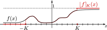
Figure 2: A profile $f$ and its saturated version $\lfloor f\rceil_{\!K}$.

Lemma II.4

Let $f,g$ be interpolating profiles and assume the PGC and that $C_{w}<\infty,$ then

$$\lim_{K\rightarrow\infty}\mathcal{W}(\lfloor f\rceil_{\!K},\lfloor g\rceil_{\!K})=\mathcal{W}(f,g)\,.$$

Proof:

See Appendix -B. ∎

We end this section with another useful definition.

• Assuming it exists, we define

  $$L(f,g)=\mathcal{W}(f,g)-\int_{\mathds{R}}(1-f^{w}(x))g(x)\,{\mathrm{d}}x\,=\int_{\mathds{R}} \mathrm{d}x\Biggl{(}\int_{0}^{f(x)}\mathrm{d}v\,h_{f}^{-1}(v)-\int_{0}^{g(x)}\mathrm{d}u\,(1-h_{g}^{-1}(u))\Biggr{)}.$$ (18)

As we will see, the functional $L(f,g)$ captures the “simple” (uncoupled) part of $\mathcal{W}:$ It is invariant under increasing rearrangements and linear under displacement interpolation.

III Rearrangements

Displacement convexity is usually defined on a space of probability measures. For measures on the real line, it is most convenient to view displacement convexity on a space of cumulative distribution functions (cdf’s). It is therefore fortunate that the search for the global minimum of the potential functional (8) can be reduced to the space of profiles $f$ and $g$ that are non-decreasing. In this section, we use the tool of increasing rearrangements to show that such rearrangements of $f$ and $g$ can only decrease the potential.

Symmetric decreasing rearrangements are a classical tool in analysis, see [22]. Here we will use a closely related cousin namely increasing rearrangements (see [23]). Our presentation is self-contained and no previous exposure to rearrangements is needed. Consider a profile $p:\mathds{R}\rightarrow[0,1]$ that satisfies (5). The increasing rearrangement of $p$ is the increasing function $\bar{p}$ that has the same limits, and where the mass of each level set is in some sense preserved (here the mass of a level set is infinite). More formally, let us represent $p$ in layer cake form as

$$p(x)=\int_{0}^{p(x)}\mathrm{d}t=\int_{0}^{1}\mathrm{d}t\,{\mathbb{1}}_{E_{t}}(x),$$ (19)

where ${\mathbb{1}}_{E_{t}}$ is the indicator function of the level set $E_{t}=\{x\,|\,p(x)>t\}$. For each value $t\in[0,1)$, the level set $E_{t}$ can be written as the disjoint union of a bounded set $A_{t}$ and a half line $(a_{t},+\infty)$. We define the rearranged set $\bar{E}_{t}=(a_{t}-|A_{t}|,+\infty)\,,$ and then

$$\bar{p}(x)=\int_{0}^{1}\mathrm{d}t\,{{\mathbb{1}}_{\bar{E_{t}}}}(x).$$ (20)

A simple example capturing the notion of increasing rearrangement is shown in Fig. 3.

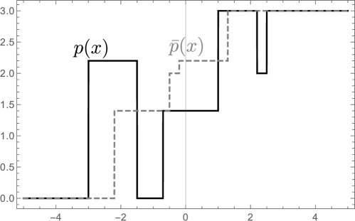
Figure 3: A simple example of an increasing rearrangement for step functions.

Lemma III.1

Let $p$ and $q$ be two profiles satisfying (5). Then, assuming the left integral exists, we have

$$\int_{\mathds{R}}\mathrm{d}x\,(p(x)-q(x))=\int_{\mathds{R}}\mathrm{d}x\,(\bar{p}(x)-\bar{q}(x))\,.$$

Proof:

For each $t\in(0,1)$ there exists a minimal $a_{t}$ such that $(a_{t},\infty)\subset\{x:p(x)>t\}\cap\{x:q(x)>t\}.$ Define $B_{p,t}=\{x:p(x)>t\}\backslash\,(a_{t},\infty)$ and $B_{q,t}=\{x:q(x)>t\}\backslash\,(a_{t},\infty).$ We also define the same quantities for the rearranged profiles $\bar{p}$ and $\bar{q}$, namely $\bar{a}_{t}$, $B_{\bar{p},t}$ and $B_{\bar{q},t}$. We show below that

$$|B_{p,t}|-|B_{q,t}|=|B_{\bar{p},t}|-|B_{\bar{q},t}|.$$ (21)

Equation (21) gives the result since, using the layer cake representation, it follows that

$$\int_{\mathds{R}}\mathrm{d}x\,(p(x)-q(x))=\int_{0}^{1}\mathrm{d}t(|B_{p,t}|-|B_{q,t}|)=\int_{0}^{1}\mathrm{d}t(|B_{\bar{p},t}|-|B_{\bar{q},t}|)=\int_{\mathds{R}}\mathrm{d}x\,(\bar{p}(x)-\bar{q}(x)).$$

Let us give an explicit argument for (21). We note that the infinite part of a level set can only increase under an increasing rearrangement, thus $(a_{t},\infty)\subset(\bar{a}_{t},\infty)$. So $(a_{t},\infty)$ is common to $\{x:\bar{p}(x)>t\}$ and $\{x:\bar{q}(x)>t\}$ and subtracting it leaves two finite sets with the same finite measure since rearrangements are measure preserving, i.e.,

$$|\{x:\bar{p}(x)>t\}\backslash\,(a_{t},\infty)|=|\{x:p(x)>t\}\backslash\,(a_{t},\infty)|,$$

(with the same $a_{t}$ on both sides). Thus,

$$|B_{\bar{p},t}| =|\{x:\bar{p}(x)>t\}\backslash\,(\bar{a}_{t},\infty)|$$

$$=|\{x:\bar{p}(x)>t\}\backslash\,(\bar{a}_{t},\infty)|-|(\bar{a}_{t},a_{t})|$$

$$=|\{x:\bar{p}(x)>t\}\backslash\,(a_{t},\infty)|-|(\bar{a}_{t},a_{t})|$$

$$=|B_{p,t}|-|(\bar{a}_{t},a_{t})|.$$

Similarly, $|B_{\bar{q},t}|=|B_{q,t}|-|(\bar{a}_{t},a_{t})|$, and (21) follows from these two identities. ∎

Lemma III.2

For any interpolating $f$ and $g$, we have

$$\int_{\mathds{R}}{\mathrm{d}}x(1-f(x))g(x)\geq\int_{\mathds{R}}{\mathrm{d}}x(1-\bar{f}(x))\bar{g}(x)$$

Proof:

If the left-hand side is infinite, then the result is immediate, so we assume that it is finite.

This result is very similar to the Hardy-Littlewood inequality for symmetric rearrangements. We will, however, give a self-contained elementary proof. The key inequality is the following which holds for all $t,s\in(0,1).$

$$\begin{split}&|\{x:1-f(x)>t\}\cap\{x:g(x)>s\}|\geq|\{x:1-\bar{f}(x)>t\}\cap\{x:\bar{g}(x)>s\}|.\end{split}$$ (22)

This gives the result since

$$\int_{\mathds{R}}{\mathrm{d}}x\,(1-f(x))g(x) =\int_{\mathds{R}}{\mathrm{d}}x\int_{0}^{1}{\mathrm{d}}t\,{\mathbb{1}}_{\{1-f(x)>t\}}(x)\int_{0}^{1}{\mathrm{d}}s\,{\mathbb{1}}_{\{g(x)>s\}}(x)$$

$$=\int_{0}^{1}\int_{0}^{1}{\mathrm{d}}t\,{\mathrm{d}}s\,|\{x:1-f(x)>t\}\cap\{x:g(x)>s\}|.$$

To see (LABEL:eqn:keyineq), observe that, for $s,t\in(0,1),$ we have some maximal $a_{t}$ and minimal $b_{s}$ such that $\{x:1-f(x)>t\}=(-\infty,a_{t})\,\,\cup A_{t}$ and $\{x:g(x)>s\}=(b_{s},+\infty)\,\,\cup B_{s}$ where the unions are disjoint and $|A_{t}|,|B_{s}|<\infty.$ If $a_{t}+|A_{t}|<b_{s}-|B_{s}|$ (see case a) in Fig. 4) then the right-hand side of (LABEL:eqn:keyineq) is $0$ and (LABEL:eqn:keyineq) is immediate, so we assume otherwise. If $a_{t}\geq b_{s}$ (see case b) in Fig. 4) then we trivially have equality in (LABEL:eqn:keyineq) so we also assume $a_{t}<b_{s}.$ We now have case c) in Fig. 4 and we obtain

$$|\{x:1-\bar{f}(x)>t\}\cap\{x:\bar{g}(x)>s\}|= |\,(-\infty,a_{t}+|A_{t}|)\,\,\cap\,\,(b_{s}-|B_{s}|,+\infty)\,|$$

$$= |A_{t}|+|B_{s}|-(b_{s}-a_{t}).$$

Note that the last line is non-negative because we are not in the case $a_{t}+|A_{t}|<b_{s}-|B_{s}|$. Now, $A_{t}$ and $B_{s}$ can intersect only in the interval $[a_{t},b_{s}]$ so we have

$$|\{x:1-f(x)>t\}\cap\{x:g(x)>s\}|= |A_{t}|+|B_{s}|-|(A_{t}\cup B_{s})\cap[a_{t},b_{s}]|$$

$$\geq |A_{t}|+|B_{s}|-(b_{s}-a_{t}),$$

and the lemma follows. ∎

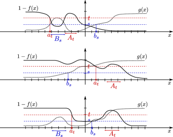
Figure 4: Illustration of level sets used in the proof of Lemma III.2. a) For $a_{t}+|A_{t}|<b_{s}-|B_{s}|$. The intersection on the right-hand side of (LABEL:eqn:keyineq) is empty and the inequality is trivial. b) For $a_{t}+|A_{t}|>b_{s}-|B_{s}|$ and $a_{t}\geq b_{s}$ (LABEL:eqn:keyineq) is an equality. c) For the last case $a_{t}+|A_{t}|>b_{s}-|B_{s}|$ and $a_{t}<b_{t}$ the inequality (LABEL:eqn:keyineq) is non-trivial.

Lemma III.3

For any interpolating $f$ and $g$, we have

$$\int_{\mathds{R}}{\mathrm{d}}x(1-f^{w}(x))g(x)\geq\int_{\mathds{R}}{\mathrm{d}}x(1-\bar{f}^{w}(x))\bar{g}(x).$$ (23)

Proof:

If the left-hand side is infinite, the inequality holds. Hence, we suppose it is finite. We have

$$\int_{\mathds{R}} {\mathrm{d}}x\,(1-f^{w}(x))g(x)=\int_{\mathds{R}}{\mathrm{d}}x\int_{\mathds{R}}{\mathrm{d}}y\,w(y)(1-f(x-y))g(x).$$

Since the integrand is non-negative and the integral is finite, we can apply the Fubini theorem to rewrite

$$\int_{\mathds{R}} {\mathrm{d}}x\,(1-f^{w}(x))g(x)=\int_{\mathds{R}}{\mathrm{d}}y\,w(y)\int_{\mathds{R}}\mathrm{d}x\,(1-f(x))g(x-y).$$ (24)

Now, we apply Lemma III.2 to the functions $f$ and $g_{y}$, where $g_{y}(x)=g(x-y)$. Note that $g_{y}$ is simply a translated version of $g$, so its rearrangement is just obtained by the same translation of $\bar{g}$, i.e., $\widebar{g_{y}}(x)=\bar{g}(x-y)$. Thus,

$$\int_{\mathds{R}}\mathrm{d}x\,(1-f(x))g(x-y)\geq\int_{\mathds{R}}\mathrm{d}x\,(1-\bar{f}(x))\bar{g}(x-y).$$

Multiplying by $w(y)$, integrating over $y$, and using (24), we obtain (23).

∎

We are now ready to prove a rearrangement inequality for $\mathcal{W}.$

Proposition III.4 (Monotonicity of Minimizers)

Let $f$ and $g$ be profiles satisfying (5) and let $\bar{f}$ and $\bar{g}$ be their respective increasing rearrangements. Assume the PGC and that $C_{w}<\infty,$ then we have

$$\mathcal{W}(f,g)\geq\mathcal{W}(\bar{f},\bar{g}).$$ (25)

Proof:

If the left-hand side of (25) is infinite, then the result is immediate, so we assume that $\mathcal{W}(f,g)$ is finite. Let us first assume that $\int_{\mathds{R}}\mathrm{d}x\,(1-f^{w}(x))g(x)<\infty$ (in fact, we can assume the saturated case). It then follows that $L(f,g)$ in Equ. (18) is finite. Note that if $F:\mathds{R}\to[0,1]$ is monotone, then $\widebar{F\circ p}=F\circ\bar{p}$. Thus the increasing rearrangement of $\int_{0}^{f(x)}\mathrm{d}v\,h^{-1}_{f}(v)$ is equal to $\int_{0}^{\bar{f}(x)}\mathrm{d}v\,h^{-1}_{f}(v)$ and similarly for the term $\int_{0}^{g(x)}\mathrm{d}u\,(1-h^{-1}_{g}(u))$. We can now apply Lemma III.1 (with suitable scaling) to conclude that $L(f,g)=L(\bar{f},\bar{g}).$ For this case, the proposition now follows from Lemma  III.3.

Now, we consider the general case, where possibly $\int_{\mathds{R}}\mathrm{d}x\,(1-f^{w}(x))g(x)=\infty$. Due to Lemma II.4, we have

$$\mathcal{W}(f,g)=\lim_{K\rightarrow\infty}\mathcal{W}(\lfloor f\rceil_{\!K},\lfloor g\rceil_{\!K}).$$ (26)

We remark that $\int_{\mathds{R}}\mathrm{d}x\,(1-(\lfloor f\rceil_{\!K}^{w}(x))\lfloor g\rceil_{\!K}(x)<\infty$ due to Lemma .2 Equ. (48). Therefore, using the saturated case, we have already established above, we have

$$\mathcal{W}(\lfloor f\rceil_{\!K},\lfloor g\rceil_{\!K})\geq W(\overline{\lfloor f\rceil_{\!K}},\overline{\lfloor g\rceil_{\!K}}).$$ (27)

Finally, it is easy to see that for any interpolating profile $f$, we have $\overline{\lfloor f\rceil_{\!K}}\rightarrow\overline{f}$ pointwise. By Lemma II.2 Equ. (12), we obtain

$$\liminf_{K\rightarrow\infty}W(\overline{\lfloor f\rceil_{\!K}},\overline{\lfloor g\rceil_{\!K}})\geq W(\bar{f},\bar{g}).$$ (28)

Combining (26), (27), and (28) concludes the proof. ∎

Proposition III.4 shows that minimizers $f$, $g$ of the functional $\mathcal{W}(f,g)$ can be found in the spaces of non-decreasing profiles. From now on, we therefore restrict the functional to those spaces.

IV Existence of Minimizers

The existence of a monotonic FP, which we will show is a minimizer of ${\mathcal{W}},$ is proved in [1]. In this section, we give an alternate proof, under similar conditions, using the direct method of the calculus of variations [24], as was done in [17].

In the direct method of the calculus of variations, one constructs a minimizer as a limit point of a minimizing sequence. Since ${\cal W}(f,g)$ is invariant under a common translation of $f$ and $g$, it is necessary to center the sequence in order to carry out the method. We can do this by translating $f$ and $g$ so that $\frac{1}{2}\in[f(0-),f(0+)].$ We call such a profile pair centered.

Proposition IV.1

Assume $C_{w}<\infty$ and assume the SPGC is satisfied. Then, there exists a monotonic non-decreasing profile pair $(f(x),g(x))$ that minimizes ${\cal W}$ under the condition that $(f,g)$ has limit $(1,1)$ at $x=\infty$ and limit $(0,0)$ at $x=-\infty.$

Proof:

We already remarked that we can adopt the alternative expression (13) for the potential functional, namely

$${\cal W}(f,g)=\int_{\mathds{R}}{\mathrm{d}}x\,\tilde{I}_{f,g,w}(x),$$

where $\tilde{I}_{f,g,w}(x)\geq 0$. Therefore ${\cal W}(f,g)$ is bounded from below so, by Proposition III.4, there exists a minimizing sequence $(f_{i},g_{i})$ of monotonic profiles satisfying the limit condition, i.e.,

$$\lim_{i\to+\infty}{\cal W}(f_{i},g_{i})=\inf\mathcal{W}(f,g).$$

Let us center the sequence so that $\frac{1}{2}\in[f_{i}(0-),f_{i}(0+)]$ for each $i.$ Interpreting $f_{i}$ and $g_{i}$ as cumulative probability distributions, our aim is to show the tightness of the sequence, i.e., that the transition of $f_{i}$ and $g_{i}$ from $\epsilon$ to $1-\epsilon$ must occur in a bounded region for all $i.$

Let $C$ be an arbitrary finite constant. Then, we claim that that for any $\epsilon>0$ there exists $Z<\infty$ such that ${\cal W}(f,g)<C$ implies that $f(x),g(x)>1-\epsilon$ for $x>Z$ and $f(x),g(x)<\epsilon$ for $x<-Z,$ (assuming $f,g$ is a centered monotonic profile pair satisfying the limit conditions).

This claim completes the proof. Indeed we can then extract from $(f_{i},g_{i})$ a subsequence $(f_{i_{k}},g_{i_{k}})$ converging to a limit point $(f_{*},g_{*})$ which necessarily satisfies the limit conditions, and by Fatou’s lemma

$$\int_{\mathds{R}}{\mathrm{d}}x\,\tilde{I}_{f_{*},g_{*},w}(x)\leq\liminf_{k\to+\infty}\int_{\mathds{R}}{\mathrm{d}}x\,\tilde{I}_{f_{i_{k}},g_{i_{k}},w}(x),$$

so $\mathcal{W}(f_{*},g_{*})\leq\inf\mathcal{W}(f,g)$ and $f_{*},g_{*}$ is a monotone minimizing pair for the potential functional.

Now we prove the claim. Since, by Lemma .3, we have

$$\int_{\mathds{R}}|f^{w}(x)-f(x)|\,dx\leq C_{w},$$

we see that ${\cal W}(f,g)<C$ implies that

$$\int_{\mathds{R}}\phi (h_{f},h_{g};g(x),f(x))\,dx=\mathcal{W}(f,g)-\int_{\mathds{R}}\mathrm{d}x\,(f(x)-f^{w}(x))g(x)\leq C+C_{w}\,.$$

By the strictly positive gap condition, there exists $\eta>0$ such that $\phi(h_{f},h_{g};g(x),f(x))>\eta$ unless we have either $f(x),g(x)<\epsilon$ or $f(x),g(x)>1-\epsilon.$ Let $x_{+}$ be the least $x$ such that $f(x),g(x)>1-\epsilon$. Then,

$$C+C_{w}\geq\int_{0}^{x_{+}}\phi (h_{f},h_{g};g(x),f(x))\,dx>\eta x_{+},$$

and $x_{+}<(C+C_{w})/\eta$. Thus for each $i$, we have $f_{i}(x),g_{i}(x)>1-\epsilon$ for $x>(C+C_{w})/\eta$. Similarly, we have for each $i$ we have $f_{i}(x),g_{i}(x)<\epsilon$ for $x<-(C+C_{w})/\eta.$ ∎

V Displacement Convexity

A generic functional $\mathcal{F}(p)$ on a space $\mathcal{X}$ (of profiles, say) is said to be convex in the usual sense if, for any pair $p_{0},p_{1}\in\mathcal{X}$, and for all $\lambda\in[0,1]$, and for the linear interpolation $(1-\lambda)p_{0}+\lambda p_{1}$ of the profiles, the inequality $\mathcal{F}((1-\lambda)p_{0}+\lambda p_{1})\leq(1-\lambda)\mathcal{F}(p_{0})+\lambda\mathcal{F}(p_{1})$ holds. Displacement convexity, on the other hand, is defined as convexity under an alternative interpolation called displacement interpolation. The usual setting for displacement convexity is a space of probability measures. For measures over the real line, one can conveniently define the displacement interpolation in terms of the cdf’s associated to the measures. This is the simplest setting and the one that we adopt here.

We think of the increasing profiles $p$ as right-continuous cdf’s of some underlying measures $\mathrm{d}p$ over the real line. As already stated, the inverse $p^{-1}(u)$ defined almost everywhere and with left and right limits $p^{-1}(u_{-})$ and $p^{-1}(u_{+})$, respectively, are uniquely defined. However, at this point, it is useful to settle on the right-continuous inverse which is defined for all $u\in(0,1)$, namely $p^{-1}(u)=\inf\{x\mid p(x)>u\}$.

Consider two profiles $p_{0}$ and $p_{1}$, and assume $p_{0}$ is continuous. We can define a map $T_{p}:\mathds{R}\to\mathds{R}$ as

$$T_{p}(x)=p_{1}^{-1}(p_{0}(x)).$$ (29)

The map $T_{p}$ can be seen as a pushforward map for measures from $\mathrm{d}p_{0}$ to $\mathrm{d}p_{1}$. This is expressed as $\mathrm{d}p_{1}=T_{p}\#\mathrm{d}p_{0}$ which means

$$\int\mathrm{d}p_{1}(x)\,h(x)=\int\mathrm{d}p_{0}(x)\,h(T_{p}(x))$$

for any function $h$ such that the integral is well-defined. Then, denoting by $id$ the identity map, the interpolant $p_{\lambda}(\cdot)$ is the cdf of the measure defined by

$$\mathrm{d}p_{\lambda}=((1-\lambda)id+\lambda T_{p})\#\mathrm{d}p_{0}.$$

We have

$$\int\mathrm{d}p_{\lambda}(x)h(x)=\int\mathrm{d}p_{0}(x)h((1-\lambda)x+\lambda T_{p}(x)),$$

whenever the integral is defined. In particular, if $h$ is convex, then this shows convexity in $\lambda$ of the integral due to the following,

$$\int\mathrm{d}p_{0}(x)h((1-\lambda)(x)+\lambda T_{p}(x)) \leq(1-\lambda)\int\mathrm{d}p_{0}(x)h(x)+\lambda\int\mathrm{d}p_{0}(x)h(T_{p}(x))$$

$$=(1-\lambda)\int\mathrm{d}p_{0}(x)h(x)+\lambda\int\mathrm{d}p_{1}(x)h(x).$$

The graphical construction of the interpolant $p_{\lambda}$ is illustrated in Fig. 5. Graphically, $T_{p}$ finds the position $x^{\prime}$ on the $x$-axis so that $p_{1}(x^{\prime})=p_{0}(x)$ for some given $x$. Consider the linear interpolation between points on $\mathds{R}$, $x_{p,\lambda}=(1-\lambda)x+\lambda T_{p}(x).$ The displacement interpolant $p_{\lambda}$ is defined so that the following equality holds for all $\lambda\in[0,1]$ $p_{\lambda}(x_{p,\lambda})=p_{0}(x).$

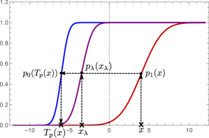
Figure 5: Monotonic profiles $p_{0}$ and $p_{1}$, the map $T_{p}(x)$, $x_{p,\lambda}=(1-\lambda)x+\lambda T_{p}(x)$, and the interpolant $p_{\lambda}$. Here, $\lambda=1/4$.

In the case where $p_{0}$ is discontinuous, we have to be more careful in the definition. At points of discontinuity of $p_{0}$, the map $T_{p}(x)$ should not be single-valued. Since we work in one dimension, this issue is easily circumvented and we can in general define $p_{\lambda}$ via its inverse as

$$p^{-1}_{\lambda}(u)=(1-\lambda)p_{0}^{-1}(u)+\lambda p_{1}^{-1}(u),$$ (30)

and $p_{\lambda}(x)=\inf\{u\mid p_{\lambda}^{-1}(u)>x\}$ (which is right continuous). Correspondingly, if $p$ is an interpolating increasing profile then, under appropriate regularity of $h,$ we can write

$$\int_{\mathds{R}}\mathrm{d}p(x)h(x)=\int_{0}^{1}\mathrm{d}u\,h(p^{-1}(u))\,$$

and we have

$$\int\mathrm{d}p_{\lambda}(x)h(x)=\int_{0}^{1}\mathrm{d}u\,h((1-\lambda)p_{0}^{-1}(u)+\lambda p_{1}^{-1}(u))\,.$$

With this in mind, we will continue to use the notation $T_{p}(x)$ when the above interpretation should be understood.

In the remainder of this work, we consider two pairs of interpolating profiles $(f_{0},f_{1})$ and $(g_{0},g_{1})$ and consider the corresponding interpolants $f_{\lambda}$ and $g_{\lambda}$.

We now state one of the main results of this paper.

Proposition V.1

Assume the PGC and $C_{w}<\infty.$ Then, the potential $\mathcal{W}(f,g)$ is displacement convex; that is, for all $\lambda\in[0,1]$,

$$\mathcal{W}(f_{\lambda},g_{\lambda})\leq(1-\lambda)\mathcal{W}(f_{0},g_{0})+\lambda\mathcal{W}(f_{1},g_{1}).$$ (31)

We first show that it is sufficient to prove the proposition under the assumption that $(f_{0},g_{0})$ and $(f_{1},g_{1})$ are saturated. We recall that by Lemma II.4, for any monotonic interpolating pair $f,g$ we have

$$\lim_{K\rightarrow\infty}\mathcal{W}(\lfloor f\rceil_{\!K},\lfloor g\rceil_{\!K})=\mathcal{W}(f,g)\,.$$ (32)

Given any monotonic interpolating pairs $(f_{0},g_{0}),(f_{1},g_{1})$, let $f_{K,\lambda}$ denote the displacement interpolant of $\lfloor f_{0}\rceil_{\!K}$ and $\lfloor f_{1}\rceil_{\!K}.$ It is easy to see that $f_{K,\lambda}$ converges pointwise to $f_{\lambda}$ when $K\to+\infty$. By Lemma II.2 Equ. (12) we therefore have

$$\liminf_{K\rightarrow\infty}\mathcal{W}(f_{K,\lambda},g_{K,\lambda})\geq\mathcal{W}(f_{\lambda},g_{\lambda})\,.$$ (33)

In view of (32) and (33), we see that (31) follows from

$$\mathcal{W}( f_{K,\lambda},g_{K,\lambda})\leq(1-\lambda)\mathcal{W}(\lfloor f_{0}\rceil_{\!K},\lfloor g_{0}\rceil_{\!K})+\lambda\mathcal{W}(\lfloor f_{1}\rceil_{\!K},\lfloor g_{1}\rceil_{\!K}).$$ (34)

which is the saturated case of (31). For the remainder of the section, we therefore assume the saturated case, and prove (34).

If $f$ and $g$ are saturated then we have

$$\int_{\mathds{R}}{\mathrm{d}}x\,(1-f^{w}(x))g(x)<\infty\,.$$

Indeed,

$$(1-f^{w}(x))g(x)=(1-f(x))g(x)+(f(x)-f^{w}(x))g(x),$$

and the first term is integrable for saturated profiles $f,g$, and the second term is also integrable because of Lemma .3 (note that $f^{w}$ is not necessarily saturated). This is the critical requirement since, by integrating by parts, we obtain

$$\int_{\mathds{R}}{\mathrm{d}}x\,(1-f^{w}(x))g(x)=\iint_{\mathds{R}^{2}}\mathrm{d}f(x)V(x-y)\mathrm{d}g(y).$$ (35)

The full derivation of this identity reads

$$\int_{\mathds{R}} {\mathrm{d}}x\,(1-f^{w}(x))g(x)=\iint_{\mathds{R}^{2}}{\mathrm{d}}x\,{\mathrm{d}}y\,(1-f(x))w(x-y)g(y)$$

$$=\iint_{\mathds{R}^{2}}\mathrm{d}f(x)\Omega(x-y)g(y)\,{\mathrm{d}}y=\iint_{\mathds{R}^{2}}\mathrm{d}f(x)V(x-y)\mathrm{d}g(y),\,$$

where we have used the fact the $V(x)$ is well-defined.

The identity (35) leads to the following key result:

Lemma V.2

Let $(f_{0},g_{0})$ and $(f_{1},g_{1})$ be saturated, then

$$\int_{\mathds{R}}{\mathrm{d}}x\,(1-f_{\lambda}^{w}(x))g_{\lambda}(x)$$

is a convex function of $\lambda.$

Proof:

Since $f_{\lambda}$ and $g_{\lambda}$ are saturated we have by (35) that

$$\int_{\mathds{R}}(1-f_{\lambda}^{w}(x))g_{\lambda}(x)\,{\mathrm{d}}x=\iint_{\mathds{R}^{2}}\mathrm{d}\!f_{\lambda}(x)V(x-y)\mathrm{d}g_{\lambda}(y)$$

$$=\iint_{\mathds{R}^{2}}\mathrm{d}\!f_{0}(x)V((1-\lambda)(x-y)+\lambda(T_{f}(x)-T_{g}(y)))\mathrm{d}g_{0}(y).$$

This is convex in $\lambda$ because the kernel $V$ is convex (see II.3). ∎

Lemma V.3

For any saturated pairs $(f_{0},g_{0}),(f_{1},g_{1}),$ the functional $L(f_{\lambda},g_{\lambda})$ is affine in $\lambda.$

Proof:

We will show that $L(f_{\lambda},g_{\lambda})-L(f_{0},g_{0})$ is linear in $\lambda$. We start by the considering the first term of this difference. Using the layer cake representation and the monotonicity of the functions, we have

$$\int_{\mathds{R}}\mathrm{d}x\Big{(}\int_{0}^{f_{\lambda}(x)}\mathrm{d}u\,h_{f}^{-1}(u)-\int_{0}^{f_{0}(x)}\mathrm{d}u\,h_{f}^{-1}(u)\Big{)} =\int_{\mathds{R}}\mathrm{d}x\,\int_{f_{0}(x)}^{f_{\lambda}(x)}\mathrm{d}u\,h_{f}^{-1}(u)$$

$$=\int_{0}^{1}\mathrm{d}u\,h_{f}^{-1}(u)(f_{0}^{-1}(u)-f_{\lambda}^{-1}(u)).$$

Using (30) we can write write this as

$$\lambda\int_{0}^{1}\mathrm{d}u\,h_{f}^{-1}(u)(f_{0}^{-1}(u)-f_{1}^{-1}(u)),$$

which is evidently linear in $\lambda$. Similarly for the second term in the difference $L(f_{\lambda},g_{\lambda})-L(f_{0},g_{0})$, we obtain

$$\int_{\mathds{R}} \mathrm{d}x\Big{(}\int_{0}^{g_{0}(x)}\mathrm{d}u\,(1-h_{g}^{-1}(u))-\int_{0}^{g_{\lambda}(x)}\mathrm{d}u\,(1-h_{g}^{-1}(u))\Big{)}$$

$$=\lambda\int_{0}^{1}\mathrm{d}u\,(1-h_{g}^{-1}(u))(g_{1}^{-1}(u)-g_{0}^{-1}(u))\,.$$

∎

We are now ready to prove the main result of this section.

Proof:

If $\mathcal{W}(f_{0},g_{0})=+\infty$ or $\mathcal{W}(f_{1},g_{1})=+\infty$, then the result is immediate, so we assume both are finite. As argued above, we can assume that all functions are saturated. We rewrite the potential in (8) as follows

$$\mathcal{W} (f_{\lambda},g_{\lambda})=L(f_{\lambda},g_{\lambda})+\int_{\mathds{R}}{\mathrm{d}}x\,(1-f_{\lambda}^{w}(x))g_{\lambda}(x).$$ (36)

By Lemma V.3, the functional $L(f_{\lambda},g_{\lambda})$ is affine and hence convex in $\lambda.$ The second term was shown to be convex in Lemma V.2. ∎

VI Fixed Points and Minimizers

The main goal of this section is to prove Proposition VI.1, which states that a pair of monotonic profiles minimizes $\mathcal{W}$ if and only if it is a “consistent” fixed point (CFP). It will be helpful to start with a preliminary discussion motivating the definition of CFP.

We already remarked that $\phi(h_{f},h_{g};u,v)$ is convex in $v$ for fixed $u$ and minimized (over $v$) by setting $v=h_{f}(u)$, and similarly for $u$ and $v$ interchanged. From (9), a similar argument shows that $I_{f,g,w}(x)\geq I_{f,h_{g}\circ f^{w},w}(x)$ and $I_{f,g,w}(x)\geq I_{h_{f}\circ g^{w},g,w}(x)$ so that

$${\cal W}(f,g)\geq{\cal W}(f,h_{g}\circ f^{w}){\rm~{}and~{}}{\cal W}(f,g)\geq{\cal W}(h_{f}\circ g^{w},g).$$

Under some conditions, we can have ${\cal W}(f,g)={\cal W}(f,h_{g}\circ f^{w})$ even though it is not the case that $g=h_{g}\circ f^{w}$ almost everywhere. This can happen, in particular, if $h_{g}$ is discontinuous and the pair $h_{f},h_{g}$ does not satisfy the strictly positive gap condition.

One of the main analytical tools used in [1] was the construction of $h_{f}$ and $h_{g}$ given $f,g,$ and $w$ so that $f,g$ form a “consistent” interpolating fixed point. Note that, from an interpolating fixed point, we can recover the graph $(u,h_{f}(u)),u\in[0,1]$ of $h_{f}$ as the parametric curve $(g^{w}(x),f(x))$ as $x\in(-\infty,+\infty).$ Given interpolating $f$ and $g$, we denote the $h_{f}$ so obtained as $h_{[f,g^{w}]}$ (see [1] for more detail.) The update function $h_{[f,g^{w}]}$ is uniquely determined at points of continuity but may not be uniquely determined at points of discontinuity. In particular, if $g^{w}$ is constant over some open interval $I$ where $f$ is increasing then $h_{[f,g^{w}]}$ has a discontinuity at that value of $g^{w}(I)$ and we see that we cannot have $f=h_{[f,g^{w}]}\circ g^{w}$ almost everywhere. Nevertheless, it is the case that $f(x)\in[h_{[f,g^{w}]}(g^{w}(x)-),h_{[f,g^{w}]}(g^{w}(x)+)]$ for all $x$ and in this sense it satisfies the DE equation. In [1], the notation

$$f\doteqdot h_{f}\circ g^{w}$$

was used to capture this case. This motivates the following definition:

• We say that an interpolating pair $f,g$ of profiles is a consistent fixed point (CFP) if $f\doteqdot h_{f}\circ g^{w}$ and $g\doteqdot h_{g}\circ f^{w}$. Recall that $f,g$ is a fixed point (FP) if $f=h_{f}\circ g^{w}$ and $g=h_{g}\circ f^{w}$ almost everywhere, i.e., up to a set of measure zero.

Proposition VI.1

Let $f,g$ be monotonic and interpolating. Then $\mathcal{W}(f,g)$ is minimal - in the sense $\mathcal{W}(f,g)\leq\mathcal{W}(f^{\prime},g^{\prime})$ for any monotonic interpolating $f^{\prime},g^{\prime}$ - if and only if $f,g$ is a CFP.

Proof:

If $f,g$ is not a CFP then either $\mathcal{W}(f,g)=\infty$ in which case the pair cannot be minimal, or we have either ${\cal W}(f,g)>{\cal W}(f,h_{g}\circ f^{w})$ or ${\cal W}(f,g)>{\cal W}(h_{f}\circ g^{w},g)$, which shows that $\mathcal{W}(f,g)$ is not minimal.

To prove the converse, assume $f_{0},g_{0}$ is a CFP. The proof proceeds by contradiction. Hence, we suppose there exists interpolating $f_{1},g_{1}$ with $\mathcal{W}(f_{0},g_{0})>\mathcal{W}(f_{1},g_{1})$ and we shall deduce a contradiction. By Lemma II.4, we can assume that $f_{1}$ and $g_{1}$ are saturated.

We will show that we may also take $f_{0},g_{0}$ to be saturated. Define

$$h_{f_{0}}^{K} =h_{[\lfloor f_{0}\rceil_{\!K},\lfloor g_{0}\rceil_{\!K}^{w}]},\quad h_{g_{0}}^{K}=h_{[\lfloor g_{0}\rceil_{\!K},\lfloor f_{0}\rceil_{\!K}^{w}]}$$

so $\lfloor f_{0}\rceil_{\!K},\lfloor g_{0}\rceil_{\!K}$ is a CFP for $h_{f_{0}}^{K},h_{g_{0}}^{K}.$ Since $f_{1},g_{1}$ are saturated, it follows easily that

$$\lim_{K\rightarrow\infty}\mathcal{W}(h_{f_{0}}^{K},h_{g_{0}}^{K};f_{1},g_{1})=\mathcal{W}(h_{f_{0}},h_{g_{0}};f_{1},g_{1})=\mathcal{W}(f_{1},g_{1}),$$

and by Lemma .4 we have

$$\lim_{K\rightarrow\infty}\mathcal{W}(h_{f_{0}}^{K},h_{g_{0}}^{K};\lfloor f_{0}\rceil_{\!K},\lfloor g_{0}\rceil_{\!K})=\mathcal{W}(f_{0},g_{0}),$$

and we see that we can assume $f_{0},g_{0}$ are saturated.

Since $f_{0},g_{0}$ is a CFP it follows that $\mathcal{W}(f_{0},g_{0})\leq\mathcal{W}(f^{\prime},g_{0})$ and $\mathcal{W}(f_{0},g_{0})\leq\mathcal{W}(f_{0},g^{\prime})$ for all interpolating $f^{\prime}$ and $g^{\prime}.$ Hence, we now have

$$\mathcal{W}(f_{\lambda},g_{\lambda})-\mathcal{W}(f_{0},g_{0}) \geq\mathcal{W}(f_{\lambda},g_{\lambda})-\mathcal{W}(f_{\lambda},g_{0})-\mathcal{W}(f_{0},g_{\lambda})+\mathcal{W}(f_{0},g_{0})$$

$$=-\int_{\mathds{R}}(f^{w}_{\lambda}(x)-f^{w}_{0}(x))(g_{\lambda}(x)-g_{0}(x))\,{\mathrm{d}}x$$

$$\geq-C\lambda^{2},$$ (37)

where $C$ is some positive constant. The last step follows from $|f^{w}_{\lambda}(x)-f^{w}_{0}(x)|\leq C_{1}\lambda$ and $\int_{\mathds{R}}{\mathrm{d}}x\,|g_{\lambda}(x)-g_{0}(x)|\,\leq C_{2}\lambda$ for some positive constants $C_{1}$ and $C_{2},$ which follows from the saturation of $f_{0},g_{0}$ and $f_{1},g_{1}.$ By Proposition V.1, we have

$$\mathcal{W}(f_{\lambda},g_{\lambda})-\mathcal{W}(f_{0},g_{0})\leq\lambda(\mathcal{W}(f_{1},g_{1})-\mathcal{W}(f_{0},g_{0})).$$ (38)

Because of the assumption on $f_{1},g_{1}$ the right-hand side of (38) is strictly negative. Thus (37) and (38) contradict each other for $\lambda$ sufficiently small. We conclude that no such $f_{1},g_{1}$ can exist. ∎

We conclude this section in Lemma VI.3 with a pleasing expression for $\mathcal{W}(f,g)$ when $f,g$ is a monotonic minimizer, equivalently a CFP. To obtain the expression, and for further application, we require a result concerning the following functional from [1],

$$\begin{split}\xi_{\phi}&(w;f,g;x_{1},x_{2})=\iint\mathrm{d}g(y)\mathrm{d}f(x)({\mathbb{1}}_{C_{1}}\Omega(x-y)+{\mathbb{1}}_{C_{2}}\Omega(y-x))\end{split}$$ (39)

where

$$C_{1}=C_{1}(x_{1},x_{2})=\{(x,y):x\leq x_{2},y>x_{1}\},\quad C_{2}=C_{2}(x_{1},x_{2})=\{(x,y):x>x_{2},y\leq x_{1}\}.$$

Note that $\xi_{\phi}$ is non-negative; this is closely related to the positive gap condition. One of the main results in [1] (Lemma 9) is the following (this result is used in Section VII).

Lemma VI.2

Let $f,g$ be a CFP for (4), then

$$\xi_{\phi}(w;f,g;x_{1},x_{2})=\phi(h_{f},h_{g};g(x_{1}+),f(x_{2}+)).$$ (40)

It turns out for our application that we only require the case $x_{1}=x_{2}$ and in this case the right-hand side of (39) simplifies, at least at points of continuity of $f$ and $g,$ to

$$\iint\mathrm{d}f(x)\mathrm{d}g(y)\,\mathbb{1}_{\{(x-x_{1})(y-x_{1})\leq 0\}}\Omega(-|x-y|).$$ (41)

Lemma VI.3

If $f,g$ is a CFP then

$$\mathcal{W}(f,g)=\iint_{\mathds{R}^{2}}\mathrm{d}f(x)\mathrm{d}g(y)\kappa(x-y),$$

where

$$\kappa(x):=V(x)-x\Omega(x)=-\int_{-\infty}^{x}yw(y)\,{\mathrm{d}}y.$$

Note that $\kappa$ is a non-negative even function that tends to $0$ at $\pm\infty$ (recall $w$ is an odd function).

Proof:

By Lemma .4, it is enough to prove this for the saturated case. For the saturated case, we can integrate by parts to obtain

$$\int_{\mathds{R}}(1-f(x))g(x)\,{\mathrm{d}}x=\iint_{\mathds{R}^{2}}\mathrm{d}\!f(x){\mathbb{1}}_{\{x-y\geq 0\}}(x-y)\mathrm{d}g(y)\,.$$

From Lemma VI.2 and (39) (or (41)) , we have

$$\int_{\mathds{R}} {\mathrm{d}}x\,\phi(h_{f},h_{g};g(x),f(x))=\iint_{\mathds{R}^{2}}\mathrm{d}f(x)|x-y|\Omega(-|x-y|)\mathrm{d}g(y)\,.$$ (42)

Combining these two equations we obtain

$$L(f,g) =\iint_{\mathds{R}^{2}}\mathrm{d}f(x)(|x-y|\Omega(-|x-y|)-{\mathbb{1}}_{\{x-y\geq 0\}}(x-y))\mathrm{d}g(y)$$

$$=-\iint_{\mathds{R}^{2}}\mathrm{d}f(x)(x-y)({\mathbb{1}}_{\{x-y\geq 0\}}-\Omega(-|x-y|))\mathrm{d}g(y)\,$$

$$=-\iint_{\mathds{R}^{2}}\mathrm{d}f(x)(x-y)\Omega(x-y)\mathrm{d}g(y)\,.$$

Adding this to (35) yields the result by the definition of $L(f,g)$ given in (18). ∎

VII Unicity of Minimizer

The existence of increasing interpolation solutions to (4) was established in [1] under the assumption of the strictly positive gap condition and assuming that $w$ is strictly positive on an interval $(-W,W),$ $W\leq+\infty$ and $0$ off of $[-W,W].$ (We shall refer to this as the interval support condition.) It was also shown in [1] that existence of such a fixed point implies the positive gap condition and, by example, it was shown that if $A(h_{f},h_{g};u)=0$ for some $u\in(0,1)$, then there may be an infinite family of fixed point solutions that are not equivalent under translation. In this section we use displacement convexity to show that the solution whose existence was proved in [1] under the strictly positive gap condition is unique up to displacement.

It follows from Proposition VI.1 that all interpolating minimizers have the same potential and that they are all CFPs. By Proposition V.1, we see that if $f_{0},g_{0}$ and $f_{1},g_{1}$ are both monotonic interpolating CFPS then $f_{\lambda},g_{\lambda}$ is a CFP for all $\lambda\in[0,1].$ Displacement convexity can therefore not be strict in this case. The aim of the proof is to show that the strictly positive gap condition then leads to the conclusion that all CFPs are equal up to translation.

Given $f_{0},g_{0}$ and $f_{1},g_{1}$, we define

$$D(u,v)=(f_{1}^{-1}(v)-g_{1}^{-1}(u))-(f_{0}^{-1}(v)-g_{0}^{-1}(u)).$$

Lemma VII.1

Let $f_{0},g_{0}$ and $f_{1},g_{1}$ be CFPs and assume the interval support condition. Then, for all $\lambda\in[0,1]$, we have

$$\mu\Bigl{\{}(u,v): \,|f_{\lambda}^{-1}(v)-g_{\lambda}^{-1}(u)|<W,D(u,v)\neq 0,\,\phi(u,v)\neq 0\Bigr{\}}=0,$$

where $\mu$ denotes 2-d Lebesgue measure.

Proof:

We assume throughout that $f_{0},g_{0}$ and $f_{1},g_{1}$ are CFPs. Formally, we have

$$\frac{\mathrm{d}^{2}}{\mathrm{d}\lambda^{2}}{\cal W}(f_{\lambda},g_{\lambda})=\iint_{[0,1]^{2}}\mathrm{d}u\mathrm{d}vD(u,v)^{2}w(f_{\lambda}^{-1}(v)-g_{\lambda}^{-1}(u)).$$

The formula is derived in Appendix -E for saturated profiles. Note that the integrand is always non-negative so the integral is well-defined, although it may take the value $+\infty.$ We claim that

$$\int_{0}^{1}\mathrm{d}\lambda\iint_{{[0,1]^{2}}}\mathrm{d}u\mathrm{d}vD(u,v)^{2}w(f_{\lambda}^{-1}(v)-g_{\lambda}^{-1}(u))=0\,.$$ (43)

Assume that the claim is false. Then there exists a set $A\subset{[0,1]^{2}}$ on which $f_{0}^{-1},g_{0}^{-1},f_{1}^{-1},g_{1}^{-1}$ are all bounded such that

$$\int_{0}^{1}\mathrm{d}\lambda\iint_{{A}}\mathrm{d}u\mathrm{d}vD(u,v)^{2}w(f_{\lambda}^{-1}(v)-g_{\lambda}^{-1}(u))=\eta>0.$$

In the saturated case, it is easy to see that ${\cal W}(f_{\lambda},g_{\lambda})$ is absolutely continuous and so is $\frac{\mathrm{d}}{\mathrm{d}\lambda}{\cal W}(f_{\lambda},g_{\lambda}).$ It now follows that for all $K$ large enough, we have

$$\int_{[0,1]}\mathrm{d}\lambda\frac{\mathrm{d}^{2}}{\mathrm{d}\lambda^{2}}{\cal W}(f_{K,\lambda},g_{K,\lambda})\geq\eta,$$

and therefore, using the convexity of ${\cal W}(f_{K,\lambda},g_{K,\lambda})$ with respect to $\lambda$, we deduce that there is a positive constant $\gamma$ such that, for all $K$ large enough, we have

$${\cal W}(\lfloor f_{0}\rceil_{\!K},\lfloor g_{0}\rceil_{\!K})+{\cal W}(\lfloor f_{1}\rceil_{\!K},\lfloor g_{1}\rceil_{\!K})-2{\cal W}({f_{K,\frac{1}{2}}},{g_{K,\frac{1}{2}}})>\gamma\,.$$

Applying Lemma II.4 and Lemma II.2(12), and noting that $f_{K,\lambda},g_{K,\lambda}$ converges pointwise to $f_{\lambda},g_{\lambda}$ yields

$${\cal W}(f_{0},g_{0})+{\cal W}(f_{1},g_{1})-2{\cal W}({f_{\frac{1}{2}}},{g_{\frac{1}{2}}})\geq\gamma,$$

which contradicts Proposition VI.1, thereby establishing the claim. Note that the claim gives the desired result except perhaps on a set of $\lambda$ of measure $0.$

Now assume that for some $\lambda\in[0,1]$ we have

$$\mu\Bigl{\{}(u,v): \,|f_{\lambda}^{-1}(v)-g_{\lambda}^{-1}(u)|<W,\,D(u,v)\neq 0,\,\phi(u,v)>0\Bigr{\}}>0.$$

By the continuity ($f_{\lambda}^{-1}$ and $g_{\lambda}^{-1}$ are continuous off of at most a countable set) and inner-regularity of Lebesgue measure, there exists a closed set $A\in(0,1)^{2}$ of positive measure and a constant $\eta>0$ such that for all $(u,v)\in A$ we have $|f_{\lambda^{\prime}}^{-1}(v)-g_{\lambda^{\prime}}^{-1}(u)|<W,$ $|D(u,v)|>\eta,$ and $\phi(u,v)>\eta$ for all $\lambda^{\prime}\in[0,1]$ satisfying $|\lambda^{\prime}-\lambda|<\eta.$

For all $\delta\in[0,2W]$, define

$$\theta(\delta)=\min_{x\in[-W+\delta,W]}(\Omega(x)-\Omega(x-\delta)).$$

Note that $\theta(\delta)>0$ for $\delta>0$ and that $\theta$ is non-decreasing.

Let us find $a<b$ such that $|a-\lambda|<\eta$ and $|b-\lambda|<\eta.$ Then, for any $(u,v)\in A,$ we have

$$\int_{a}^{b}\mathrm{d}\lambda D (u,v)^{2}w(f_{0}^{-1}(v)-g_{0}^{-1}(u)+\lambda D(u,v))$$

$$=D(u,v)\big{[}\Omega(f_{0}^{-1}(v)-g_{0}^{-1}(u)+bD(u,v))-\Omega(f_{0}^{-1}(v)-g_{0}^{-1}(u)+aD(u,v))\big{]}$$

$$\geq|D(u,v)|\,\theta((b-a)|D(u,v)|)$$

$$\geq\eta\,\theta((b-a)\eta).$$

By the Fubini theorem, this contradicts our above established claim (43). ∎

Let us define $D_{W}=\{(u,v):|f^{-1}(v)-g^{-1}(u)|<W\}$ and let $B_{\epsilon}(u)$ denote the open interval centered at $u$ of length $2\epsilon.$

Lemma VII.2

Let $f,g$ be a CFP and assume the SPGC and the interval support condition. For all $v\in(0,1)$, there exists $u\in(0,1)$ and $\epsilon>0$ such that $B_{\epsilon}(u)\times B_{\epsilon}(v)\subset D_{W}.$

Proof:

Let $v\in(0,1)$ and define $x_{m}=\frac{1}{2}(f^{-1}(v+)+f^{-1}(v-)).$ We must have $f^{-1}(v+)-f^{-1}(v-)<2W$ since, otherwise, we obtain $\xi_{\phi}(w;f,g;x_{m},x_{m})=0$ which, by Lemma VI.2, contradicts the SPGC.

To be more precise, for $z\in\mathds{R}$, let us define

$$T_{1}(z) =C_{1}(z,z)\cap\{|x-y|<W\}=\{(x,y):x>z,y\leq z,x-y<W\},$$

$$T_{2}(z) =C_{2}(z,z)\cap\{|x-y|<W\}=\{(x,y):x\leq z,y>z,y-x<W\}.$$

By (39) (see also (41)), the SPGC implies that the $\mathrm{d}f\mathrm{d}g$ measure of at least one of $T_{1}(x_{m})$ and $T_{2}(x_{m})$ is strictly positive. We shall assume that the measure of $T_{1}(x_{m})$ is positive, and the other case can be handled similarly. It follows from monotonicity of $f$ and $g$ that there exists $u\in(0,1)$ and $\epsilon$ sufficiently small such that $g^{-1}(B_{\epsilon}(u))\times f^{-1}((v,v+\epsilon))\subset T_{1}(x_{m}).$ We then have $g^{-1}(B_{\epsilon}(u))\subset(x_{m}-W,x_{m}]$ and, for $\epsilon$ small enough, $f^{-1}((v-\epsilon,v))\subset(x_{m}-W,x_{m}]$, which gives $B_{\epsilon}(u)\times B_{\epsilon}(v)\subset D_{W}.$ ∎

By Lemma VII.1, we have that, if $f_{0},g_{0}$ and $f_{1},g_{1}$ are CFPs and the SPGC and interval support condition holds, then

$$\mu\{(u,v):|f_{\lambda}^{-1}(v)-g_{\lambda}^{-1}(u)|<W,D(u,v)\neq 0\}=0.$$ (44)

We claim that this implies that $f_{1}^{-1}(v)-f_{0}^{-1}(v)$ is essentially constant. Similarly, we have $g_{1}^{-1}(u)-g_{0}^{-1}(u)$ is essentially constant. Moreover, these two constants are equal.

Lemma VII.3

Assume the SPGC and the interval support condition and that $f_{1},g_{1}$ and $f_{0},g_{0}$ are CFPs. Then, $f_{1}^{-1}-f_{0}^{-1}$ is essentially constant on $[0,1].$

Proof:

Let us assume that $D_{f}=f_{1}^{-1}-f_{0}^{-1}$ is not essentially constant, i.e., there exists a real value $s$ so that $|\{v:D_{f}(v)>s\}|\in(0,1)$ and $|\{v:D_{f}(v)\leq s\}|\in(0,1)$. Then, there exists a value $v^{*}\in(0,1)$ that is in the support of both sets, i.e., for any $\epsilon>0$ we have $|\{v:D_{f}(v)>s\}\cap B_{\epsilon}(v^{*})|>0$ and $|\{v:D_{f}(v)\leq s\}\cap B_{\epsilon}(v^{*})|>0.$

By Lemma VII.2, there exists a $u\in(0,1)$ and $\epsilon>0$ such that $B_{\epsilon}(u)\times B_{\epsilon}(v^{*})\subset D_{W}.$ By definition of $v^{*}$, there is a positive constant $\eta>0$ such that $\int_{B_{\epsilon}(v^{*})}{\mathrm{d}}v\,|D(u,v)|>\eta$ for all $u\in B_{\epsilon}(u)$, which now contradicts (44). This completes the proof. ∎

Proposition VII.4

Assume the SPGC and the interval support condition and that $f_{1},g_{1}$ and $f_{0},g_{0}$ are interpolating monotonic CFPs. Then, there exists $m$ such that, for almost all $x$, we have $f_{1}(x)=f_{0}(x+m)$ and $g_{1}(x)=g_{0}(x+m).$

Proof:

By Lemma VII.3, there exists $m$ such that $f_{1}^{-1}(v)-f_{0}^{-1}(v)=m$ for almost all $v\in[0,1].$ Similarly, there exists $m^{\prime}$ such that $g_{1}^{-1}(u)-g_{0}^{-1}(u)=m^{\prime}$ for almost all $u\in[0,1].$ It follows that $D(u,v)=m-m^{\prime}$ for almost all $(u,v)\in[0,1]^{2}.$ It now follows from Lemma VII.2 and (44) that $m=m^{\prime}.$ ∎

Even though we have stated and proved the results for CFPs, under the assumptions of this section CFPs are actually FPs.

Lemma VII.5

If $f,g$ is a CFP and $h_{f},h_{g}$ satisfies the strictly positive gap condition and the interval support condition holds, then $f,g$ is a FP.

Proof:

If the SPGC and the interval support condition hold then $f^{w}$ and $g^{w}$ are strictly increasing wherever they take values in $(0,1).$ This implies that $f,g$ must be a FP (see [1] for further detail). ∎

VIII Illustrations

In this work, we have shown (Proposition IV.1 and Propositions V.1, VI.1, and VII.4) that under some conditions, the potential functional $\mathcal{W}$ is displacement convex and that its minimizer exists and is unique up to translation. These conditions are the strictly positive gap condition, $C_{w}<\infty$, and the interval support condition. In this section, we apply these results on different scalar systems when these conditions hold. In particular, for the applications we consider, we use the even uniform window with $W=\frac{1}{2}$ which implies the two latter conditions. We illustrate for each application that the strictly positive gap condition holds.

To check the SPGC one can directly look at $\phi(h_{f},h_{g};u,v)$, but there is also a simpler way to check the condition. Indeed, we already remarked that for fixed $u$ the potential is minimized by setting $v=h_{f}(u)$. Therefore,

$$\phi(h_{f},h_{g};u,v)\geq\phi(h_{f},h_{g};u,h_{f}(u))=A(h_{f},h_{g};u).$$

So the SPGC is valid as long as the signed area $A(h_{f},h_{g};u)>0$ for $u\in(0,1)$. Similarly, for fixed $v$, the potential is minimized by setting $u=h_{g}(v)$. Thus,

$$\phi(h_{f},h_{g};u,v)\geq\phi(h_{f},h_{g};h_{g}(v),v)=\tilde{A}(h_{f},h_{g};v),$$

where

$$\tilde{A}(h_{f},h_{g};v)=\int_{0}^{v}dv^{\prime}(h_{f}^{-1}(v^{\prime})-h_{g}(v^{\prime}))$$

is the alternative signed area bounded between the two EXIT curves and the horizontal axis at the origin and at height $v$. The SPGC is valid as long as $\tilde{A}(h_{f},h_{g};v)>0$ for $v\in(0,1)$.

Clearly, when $\phi(h_{f},h_{g};1,1)=0$ as assumed in this paper, we also have $A(h_{f},h_{g};1)=\tilde{A}(h_{f},h_{g};1)$.

VIII-A LDPC Code Ensembles on the BEC

We demonstrate our results on the $(3,6)$-regular spatially coupled LDPC code ensemble when transmission takes place over the BEC($\epsilon$). For this ensemble, we have the (unscaled) uncoupled DE equations $\mathrm{x}=\epsilon\mathrm{y}^{2}$ and $\mathrm{y}=1-(1-\mathrm{x})^{5}$. We already showed how to perform the right scaling $\mathrm{x}=\mathrm{x}_{\text{\tiny MAP}}v$ and $\mathrm{y}=\mathrm{y}_{\text{\tiny MAP}}u$; asking that $(u,v)=(1,1)$ is a fixed point and $A(h_{f},h_{g};1)=0$ we find $\mathrm{y}_{\text{\tiny MAP}}=0.941$, $\mathrm{x}_{\text{\tiny MAP}}=0.432$ and $\epsilon=\epsilon_{\text{\tiny MAP}}=0.4881$. Replacing these numbers in the expression of the potential function (see Section  II-A) we find $\phi(u,v)$. Fig. 6 and 7 illustrate the corresponding EXIT curves and the potential that is seen to satisfy the SPGC.

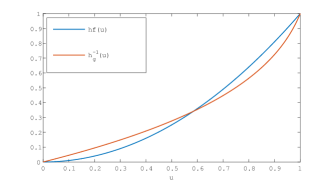
Figure 6: We plot the EXIT curves $h_{f}(u)$ and $h_{g}^{-1}(u)$ for $u\in[0,1]$ for the $(3,6)$-regular LDPC ensemble with transmission over the BEC(0.4881). We note that the signed area between the curves is equal to zero.

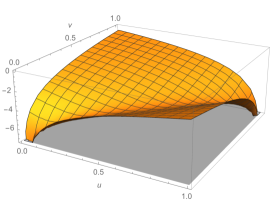
Figure 7: We consider the $(3,6)$-regular LDPC ensemble with transmission over the BEC($\epsilon$). We plot $\phi(h_{f},h_{g};u,v)$ for $(u,v)\in[0,1]^{2}$ in log scale when $\epsilon=\epsilon_{\text{\tiny MAP}}=0.4881$. We can see that $\phi(h_{f},h_{g};u,v)>0$ for $(u,v)\in(0,1)^{2}$ and $\phi(h_{f},h_{g};0,0)=\phi(h_{f},h_{g};1,1)=0$.

VIII-B Generalized LDPC Codes

We consider a generalized LDPC (GLDPC) code, where the check node constraints are given by a primitive BCH code with minimum distance $d=2e+1$ (see [25] for more information). We consider the code with degree-2 variable nodes and degree-$n$ check nodes, with transmission over the BEC($\epsilon$). The (unscaled) uncoupled DE equations are [12]

$$\begin{cases}\mathrm{x}=\epsilon\mathrm{y},\\ \mathrm{y}=\sum_{i=e}^{n-1}{n-1\choose i}\mathrm{x}^{i}(1-\mathrm{x})^{n-i-1}.\end{cases}$$

Set $\epsilon=\epsilon_{\text{\tiny MAP}}$ and $\mathrm{y}=\mathrm{y}_{\text{\tiny MAP}}u$, $\mathrm{x}=\mathrm{x}_{\text{\tiny MAP}}v$. We then get the scaled equations (1), namely $v=h_{f}(u)$, $u=h_{g}(v)$

$$\begin{cases}h_{f}(u)=\epsilon_{\text{\tiny MAP}}\mathrm{x}_{\text{\tiny MAP}}^{-1}\mathrm{y}_{\text{\tiny MAP}}u,\\ h_{g}(v)=\mathrm{y}_{\text{\tiny MAP}}^{-1}\sum_{i=e}^{n-1}{n-1\choose i}\mathrm{x}_{\text{\tiny MAP}}^{i}\mathrm{v}^{i}(1-\mathrm{x}_{\text{\tiny MAP}}v)^{n-i-1}.\end{cases}$$

The normalization condition $h_{f}(1)=h_{g}(1)=1$ and the condition $\tilde{A}(h_{f},h_{g};1)=0$ completely determine $\epsilon_{\text{\tiny MAP}}$, $\mathrm{x}_{\text{\tiny MAP}}$, and $\mathrm{y}_{\text{\tiny MAP}}$. The potential function and (alternative) signed area are given by

$$\phi(u,v) =\frac{\mathrm{x}_{\text{\tiny MAP}}u^{2}}{2\epsilon_{\text{\tiny MAP}}\mathrm{y}_{\text{\tiny MAP}}}+\int_{0}^{v}\mathrm{d}v^{\prime}\,h_{g}^{-1}(v^{\prime})-uv.$$

$$\tilde{A}(h_{f},h_{g};v) =\frac{\mathrm{x}_{\text{\tiny MAP}}v^{2}}{2\epsilon_{\text{\tiny MAP}}\mathrm{y}_{\text{\tiny MAP}}}-\frac{1}{\mathrm{y}_{\text{\tiny MAP}}}\sum\limits_{i=e}^{n-1}\sum\limits_{m=0}^{n-i-1}{n-1\choose i}{n-i-1\choose m}\frac{\mathrm{x}_{\text{\tiny MAP}}^{m+i}v^{m+i+1}}{m+i+1}.$$

The EXIT curves and signed area are illustrated in Fig. 8. and Fig. 9 for the GLDPC code with $n=15$ and $e=3$. This corresponds to $\mathrm{x}_{\text{\tiny MAP}}=0.3670$, $y_{\text{\tiny MAP}}=0.9342$, $\epsilon_{\text{\tiny MAP}}=0.3901$. Clearly, the SPGC condition is satisfied.

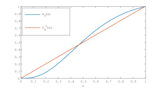
Figure 8: We plot the EXIT curves $h_{f}(u)$ and $h_{g}^{-1}(u)$ for $u\in[0,1]$ for the GLDPC code with $n=15$ and $e=3$, when transmission takes place over the BEC(0.3901). We note that the signed area between the curves is equal to zero.

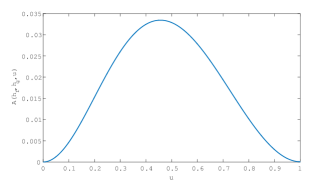
Figure 9: We consider the GLDPC code with $n=15$ and $e=3$, with transmission over the BEC($\epsilon$). We plot $\tilde{A}(h_{f},h_{g};v)$ for $v\in[0,1]$ when the channel parameter is $\epsilon=\epsilon_{\text{\tiny MAP}}=0.3901$.

VIII-C The Gaussian Approximation

There are various forms of the Gaussian approximation [26], [27], [28] used to simplify the analysis of coding systems with transmission over binary memoryless symmetric (BMS) channels. Here, we consider a variant developed in [27], [28]. This method approximates the densities of the log-likelihood ratio (LLR) messages exchanged in the decoding graph with symmetric Gaussian densities; that is, densities of the form $\mathtt{x}(\alpha)=1/\sqrt{2\pi\sigma^{2}}\exp(-\frac{(\alpha-m)^{2}}{2\sigma^{2}})$ with the property $\sigma^{2}=2m$. We also approximate the BMS channel $\mathtt{c}$ with a binary-input Gaussian additive white noise (BIGAWN) channel with parameter $\sigma^{2}$ and with the same entropy $H(\mathtt{c})$ as the original channel $\mathtt{c}$. This makes the analysis one-dimensional and has been shown to serve as a good approximation.

The Gaussian approximation allows us to track the evolution of decoding by tracking the entropies of the LLR messages. Let $\psi(m)$ denote the entropy of a symmetric Gaussian density of mean $m$ [29]. In particular, it can be expressed as

$$\psi(m)=\frac{1}{\sqrt{4\pi m}}\int_{\mathds{R}}\mathrm{d}z\,e^{-\frac{(z-m)^{2}}{4m}}\log_{2}(1+e^{-z}).$$

Note that $\psi(+\infty)=0$ and $\psi(0)=1$. We consider the $(3,6)$-regular LDPC code ensemble with transmission over the BMS.

The (unscaled) uncoupled DE equations are

$$\begin{cases}\mathrm{x}=\psi(\psi^{-1}(H(\mathtt{c}))+2\psi^{-1}(\mathrm{y})),\\ \mathrm{y}=1-\psi(5\psi^{-1}(1-\mathrm{x})).\end{cases}$$

We define $m_{\text{\tiny MAP}}$ as the value of $\psi^{-1}(H(\mathtt{c}))$ at the MAP threshold and set $\psi^{-1}(H(\mathtt{c}))=m_{\text{\tiny MAP}}$ and $\mathrm{x}=\mathrm{x}_{\text{\tiny MAP}}v$, $\mathrm{y}=\mathrm{y}_{\text{\tiny MAP}}u$. We then get the scaled equations (1), namely $v=h_{f}(u)$, $u=h_{g}(v)$

$$\begin{cases}h_{f}(u)=\mathrm{x}_{\text{\tiny MAP}}^{-1}\psi(m_{\text{\tiny MAP}}+2\psi^{-1}(\mathrm{y}_{\text{\tiny MAP}}u)),\\ h_{g}(v)=\mathrm{y}_{\text{\tiny MAP}}^{-1}-\mathrm{y}_{\text{\tiny MAP}}^{-1}\psi(5\psi^{-1}(1-\mathrm{x}_{\text{\tiny MAP}}v)).\end{cases}$$

The normalization condition $h_{f}(1)=h_{g}(1)=1$ and the condition $\tilde{A}(h_{f},h_{g};1)=0$ completely determine $m_{\text{\tiny MAP}}$, $\mathrm{x}_{\text{\tiny MAP}}$, and $\mathrm{y}_{\text{\tiny MAP}}$. The potential function is given by

$$\phi(u,v)= u(\mathrm{x}_{\text{\tiny MAP}}^{-1}-v)+\mathrm{x}_{\text{\tiny MAP}}^{-1}\int_{0}^{u}\mathrm{d}u^{\prime}\,\psi\Big{(}\frac{1}{5}\psi^{-1}(1-\mathrm{y}_{\text{\tiny MAP}}u^{\prime})\Big{)}+\mathrm{y}_{\text{\tiny MAP}}^{-1}\int_{0}^{u}\mathrm{d}v^{\prime}\,\psi\Big{(}\frac{1}{2}\psi^{-1}(\mathrm{x}_{\text{\tiny MAP}}v^{\prime})-\frac{1}{2}m_{\text{\tiny MAP}}\Big{)}.$$

A plot of the EXIT curves and potential function yields curves that are very similar to the case of the BEC (see e.g. Figs 6, 7).

VIII-D Compressive Sensing

Consider a signal vector $\mathbf{s}$ of length $n$ where the components are i.i.d. copies of a random variable $S$. We assume that $\mathbb{E}[S^{2}]=1$ and that each component of $\mathbf{s}$ is corrupted with Gaussian noise $\mathcal{N}(0,\sigma^{2}=1/\mathtt{snr})$. We take $m$ measurements of the signal and assume that the measurement matrix has i.i.d. Gaussian components $\mathcal{N}(0,1/\sqrt{n})$. The measurement ratio is defined by $\delta=m/n$. Here we are interested in state evolution [6], which tracks the mean square error of the approximate message-passing (AMP) estimator (for the signal) . Given an $\mathtt{snr}$ that is large enough, the parameter $\delta$ is kept fixed as $n$ gets large.

The state evolution fixed point equations read

$$\begin{cases}\mathrm{y}=(\frac{1}{\mathtt{snr}}+\frac{\mathrm{x}}{\delta})^{-1},\\ \mathrm{x}=\mathtt{mmse}(\mathrm{y}),\end{cases}$$ (45)

where the minimum mean square error function $\mathtt{mmse}$ is defined as follows. Let $Y=\sqrt{\mathtt{snr}}S+Z$ where $Y$ is a scalar output and $Z\sim\mathcal{N}(0,1)$ and let $\hat{S}(Y,\mathtt{snr})=\mathbb{E}_{S|Y}[S|Y]$. Then $\mathtt{mmse}(\mathtt{snr})=\mathbb{E}_{S,Y}[(S-\hat{S}(Y,\mathtt{snr}))^{2}]$. In the equations above, when we initialize with $x^{(0)}=1$, $x^{(t)}$ is the average mean square error of the AMP estimator at iteration $t$.

We now put this system of equations in the form (1). Here, there is no trivial fixed point $\mathrm{x}=\mathrm{y}=0$; however, the picture is very similar to LDPC coding-like systems considered above. The role of the “trivial” fixed point is played by a fixed point $\mathrm{x}_{*},\mathrm{y}_{*}$ obtained by initializing state evolution with $\mathrm{x}=0$. Given the $\mathtt{snr}$, for $\delta$ below the algorithmic threshold, this is the only fixed point, and for $\delta$ above this threshold, one finds three solutions (besides $\mathrm{x}_{*},\mathrm{y}_{*}$ which is stable, there are an unstable and a stable fixed point). Set $\mathrm{x}^{\prime}=\mathrm{x}-\mathrm{x}_{*}$ and $\mathrm{y}^{\prime}=\mathrm{y}-\mathrm{y}_{*}$. Equations (45) become

$$\begin{cases}\mathrm{y}^{\prime}=-\mathrm{y}_{*}+(\frac{1}{\mathtt{snr}}+\frac{\mathrm{x}_{*}+\mathrm{x}^{\prime}}{\delta})^{-1},\\ \mathrm{x}^{\prime}=-\mathrm{x}_{*}+\mathtt{mmse}(\mathrm{y}_{*}+\mathrm{y}^{\prime}).\end{cases}$$ (46)

Note that $\mathrm{x}^{\prime}=\mathrm{y}^{\prime}=0$ is a fixed point. We now scale $\mathrm{x}^{\prime}=\mathrm{x}_{\text{\tiny MAP}}v$, $\mathrm{y}^{\prime}=\mathrm{y}_{\text{\tiny MAP}}u$ where $\mathrm{x}_{\text{\tiny MAP}}$ and $\mathrm{y}_{\text{\tiny MAP}}$ are chosen later on. Then (46) takes the form (1) with the EXIT curves defined as

$$\begin{cases}h_{g}(v)=-\mathrm{y}_{*}\mathrm{y}_{\text{\tiny MAP}}^{-1}+(\frac{1}{\mathtt{snr}}+\frac{\mathrm{x}_{*}+\mathrm{x}_{\text{\tiny MAP}}v}{\delta})^{-1}\mathrm{y}_{\text{\tiny MAP}}^{-1},\\ h_{f}(u)=-\mathrm{x}_{*}\mathrm{x}_{\text{\tiny MAP}}^{-1}+\mathtt{mmse}(\mathrm{y}_{*}+\mathrm{y}_{\text{\tiny MAP}}u)\mathrm{x}_{\text{\tiny MAP}}^{-1}.\end{cases}$$ (47)

From these, one can compute the potential and the signed areas. Here, we illustrate the signed area. We have

$$h_{g}^{-1}(u)=-\mathrm{x}_{*}\mathrm{x}_{\text{\tiny MAP}}^{-1}+\delta((\mathrm{y}_{*}+\mathrm{y}_{\text{\tiny MAP}}u)^{-1}+\mathtt{snr}^{-1}),$$

from which it follows that

$$A(h_{f},h_{g};u)= \frac{\delta}{\mathrm{x}_{\text{\tiny MAP}}\mathrm{y}_{\text{\tiny MAP}}}\ln(1+\frac{\mathrm{y}_{\text{\tiny MAP}}}{\mathrm{y}_{*}}u)+\frac{u\delta}{\mathrm{x}_{\text{\tiny MAP}}\mathtt{snr}}-\frac{1}{\mathrm{x}_{\text{\tiny MAP}}}\int_{0}^{u}\mathrm{d}u^{\prime}\,\mathtt{mmse}(\mathrm{y}_{*}+\mathrm{y}_{\text{\tiny MAP}}u^{\prime})$$

Finally, we set the signal-to-noise ratio to the value $\mathtt{snr}_{\text{\tiny MAP}}$ defined such that $h_{f}(1)=h_{g}(1)=1$ and $A(h_{f},h_{g};1)|_{\mathtt{snr}_{\text{\tiny MAP}}}=0$. These conditions also determine $\mathrm{x}_{\text{\tiny MAP}}$ and $\mathrm{y}_{\text{\tiny MAP}}$ (note also that these values are a “non-trivial” stable fixed point). A plot of $A(h_{f},h_{g};u)|_{\mathtt{snr}_{\text{\tiny MAP}}}$ at $\mathtt{snr}_{\text{\tiny MAP}}$ yields a curve similar to Fig. 9 that satisfies the SPGC.

IX Conclusion

There are some questions that remain open. We have seen in Section III that we restrict our search of minimizing profiles to the space of increasing profiles. It is not clear in our settings when the inequality (25) is strict and so we cannot exclude the existence of a minimizing pair outside the spaces of increasing profiles. Another more fundamental open problem comes back to our formulation of the potential. In applications, it is inherently discrete whereas in our analysis, it is convenient to consider the continuum limit approximation of the potential. It would be interesting to see whether this analysis can be adapted to the discrete formulation.

References

[1]
S. Kudekar, T. Richardson, and R. L. Urbanke, “Wave-like solutions of general
one-dimensional spatially coupled systems,” IEEE Transcations on
Information Theory, vol. 61, no. 8, pp. 4117–4157, 2015.
[2]
A. J. Felstrom and K. S. Zigangirov, “Time-Varying Periodic Convolutional
Codes With Low-Density Parity-Check Matrix,” IEEE Transactions on
Information Theory, pp. 2181–2190, 1999.
[3]
M. Lentmaier, A. Sridharan, K. S. Zigangirov, and D. J. Costello Jr,
“Terminated LDPC convolutional codes with thresholds close to capacity,”
in IEEE International Symposium on Information Theory Proceedings
(ISIT). IEEE, 2005, pp. 1372–1376.
[4]
M. Lentmaier, A. Sridharan, D. J. Costello Jr, and K. Zigangirov, “Iterative
decoding threshold analysis for LDPC convolutional codes,” IEEE
Transactions on Information Theory, vol. 56, no. 10, pp. 5274–5289, 2010.
[5]
S. Kudekar, T. Richardson, and R. L. Urbanke, “Spatially coupled ensembles
universally achieve capacity under belief propagation,” IEEE
Transactions on Information Theory, vol. 59, no. 12, pp. 7761–7813, 2013.
[6]
D. L. Donoho, A. Javanmard, and A. Montanari, “Information-theoretically
optimal compressed sensing via spatial coupling and approximate message
passing,” in IEEE International Symposium on Information Theory
Proceedings (ISIT). IEEE, 2012, pp.
1231–1235.
[7]
F. Krzakala, M. Mézard, F. Sausset, Y. Sun, and L. Zdeborová,
“Probabilistic reconstruction in compressed sensing: algorithms, phase
diagrams, and threshold achieving matrices,” Journal of Statistical
Mechanics: Theory and Experiment, vol. 2012, no. 08, p. P08009, 2012.
[8]
S. H. Hassani, N. Macris, and R. Urbanke, “Coupled Graphical Models and Their
Thresholds,” in Information Theory Workshop (ITW), 2010, pp. 1–5.
[9]
——, “Chains of Mean Field Models,” Journal of Statistical
Mechanics: Theory and Experiment P02011, pp. 1–5, 2012.
[10]
——, “Threshold saturation in spatially coupled constraint satisfaction
problems,” Journal of Statistical Physics, vol. 150, no. 5, pp.
807–850, 2013.
[11]
D. Achlioptas, S. H. Hassani, N. Macris, and R. Urbanke, “Bounds for random
constraint satisfaction problems via spatial coupling,” in Proceedings
of the Twenty-Seventh Annual ACM-SIAM Symposium on Discrete
Algorithms. SODA, 2016, pp. 469–479.
[12]
A. Yedla, Y.-Y. Jian, P. S. Nguyen, and H. D. Pfister, “A simple proof of
Maxwell saturation for coupled scalar recursions,” IEEE Transactions
on Information Theory, vol. 60, no. 11, pp. 6943–6965, 2014.
[13]
S. Kumar, A. J. Young, N. Macris, and H. D. Pfister, “Threshold Saturation
for Spatially Coupled LDPC and LDGM Codes on BMS Channels,” IEEE
Transactions on Information Theory, vol. 60, no. 12, pp. 7389–7415, 2014.
[14]
A. Giurgiu, N. Macris, and R. Urbanke, “Spatial coupling as a proof technique
and three applications,” IEEE Transcations on Information Theory,
vol. 62, no. 10, pp. 5281–5295, 2016.
[15]
J. Barbier, M. Dia, N. Macris, F. Krzakala, T. Lesieur, and L. Zdeborova,
“Mutual information for symmetric rank-one matrix estimation: A proof of the
replica formula,” Neural Information processing Systems (NIPS), 2016.
[16]
R. El-Khatib, N. Macris, and R. Urbanke, “Displacement convexity, a useful
framework for the study of spatially coupled codes,” in Information
Theory Workshop (ITW). IEEE, 2013,
pp. 1–5.
[17]