Loading a linear Paul trap to saturation from a magneto-optical trap

Abstract

We present experimental measurements of the steady-state ion number in a linear Paul trap (LPT) as a function of the ion-loading rate. These measurements, taken with (a) constant Paul trap stability parameter $q$, (b) constant radio-frequency (rf) amplitude, or (c) constant rf frequency, show nonlinear behavior. At the loading rates achieved in this experiment, a plot of the steady-state ion number as a function of loading rate has two regions: a monotonic rise (region I) followed by a plateau (region II). Also described are simulations and analytical theory which match the experimental results. Region I is caused by rf heating and is fundamentally due to the time dependence of the rf Paul-trap forces. We show that the time-independent pseudopotential, frequently used in the analytical investigation of trapping experiments, cannot explain region I, but explains the plateau in region II and can be used to predict the steady-state ion number in that region. An important feature of our experimental LPT is the existence of a radial cut-off $\hat{R}_{\rm cut}$ that limits the ion capacity of our LPT and features prominently in the analytical and numerical analysis of our LPT-loading results. We explain the dynamical origin of $\hat{R}_{\rm cut}$ and relate it to the chaos border of the fractal of non-escaping trajectories in our LPT. We also present an improved model of LPT ion-loading as a function of time.

I Introduction

The loading dynamics of the linear Paul trap (LPT) are of interest in relation to recent work measuring the total charge exchange and elastic collision rate of atomic ions with their parent atoms in a hybrid trap Lee et al. (2013); Goodman et al. (2015). In these hybrid-trap measurements of collisions between atoms and dark ions, those without optically accessible transitions, the fluorescence of the atoms in the MOT was monitored in the presence of trapped ions. Knowledge of both the number of trapped ions and the size of the ion cloud is necessary for finding the total interaction rate. Both of these papers attempted to create a model for the loading of ions into a Paul trap. However, neither group was able to create a satisfactory model of Paul trap loading. This paper aims to understand and model the loading of a linear Paul trap at the conditions used in current hybrid trap experiments.

Hybrid traps consist of a neutral atom trap coincident with an ion trap. A variety of neutral atom traps have been used in hybrid trap experiments: magnetic traps Zipkes et al. (2010a, b); Schmid et al. (2010), magneto-optical traps (MOT) Grier et al. (2009); Rellergert et al. (2011); Hall et al. (2011); Ravi et al. (2012a); Deiglmayr et al. (2012); Sivarajah et al. (2012); Hall et al. (2013); Lee et al. (2013); Haze et al. (2013); Smith et al. (2014); Haze et al. (2015); Goodman et al. (2015), and optical dipole traps Härter et al. (2012); Krükow et al. (2016); Meir et al. (2016). In contrast, every hybrid trap experiment listed above used a Paul trap to hold the ionic species, except Deiglmayr et al. (2012), which used an octupole trap.

In hybrid trap experiments for dark ions and their parent atoms, the ion-atom total elastic and inelastic interaction rate per atom $\gamma_{\mathrm{ia}}$ is given by Goodman et al. (2015)

$$\gamma_{\mathrm{ia}}=\frac{k_{\mathrm{ia}}N_{I}C}{V_{\mathrm{ia}}}.$$ (1)

In this equation $k_{\mathrm{ia}}$ is the total elastic and charge-exchange collision rate constant, $N_{I}$ is the average number of trapped ions overlapping the atom cloud, $C$ is a function that describes the concentricity of the atom and ion clouds, and $V_{\mathrm{ia}}$ is the effective overlap volume of the two clouds Goodman et al. (2015).

In these experiments the ion trap is saturated, which has two benefits. The first is that this maximizes the rate and thus the experimental resolution of the rate constant, $k_{\mathrm{ia}}$, because the ion number and volume will be as large as possible.

The second benefit to a saturated ion trap is that the ion number, the concentricity, and the overlap volume will all be time independent on average. In the case of dark ions, the ion number can only be measured destructively; this measurement would be extremely difficult if the ion number were time dependent. For bright ions, those with optical transitions, these quantities could be measured in a time dependent way using the fluorescence. Typically, however, bright ion experiments have focused on the charge-exchange rate constant and have not measured the total rate. If the technique described in Lee et al. (2013); Goodman et al. (2015) were used in conjunction with the methods for measuring the charge exchange rate constant, then the elastic rate constant could be found as well.

Neither of the dark ion experiments developed a satisfactory model for predicting the steady-state population of the saturated Paul trap as a function of the ionization rate. In the model used in Lee, et  al. Lee et al. (2013), an ad hoc term was required to prevent the ion number from becoming infinite at large photoionization intensities and $\gamma_{\mathrm{ia}}$ was proportional to the Paul trap loss rate $\ell$. In Goodman, et  al. Goodman et al. (2015), we found experimentally that $\gamma_{\mathrm{ia}}$ was not proportional to $\ell$. We also found, by considering how the number of atoms in the MOT depended on the photoionization intensity, that the equation for the ion number as a function of photoionization intensity is naturally finite as the photoionization intensity tends to infinity.

Ion loading in a Paul trap as a function of time is typically fit to the solution of

$$\frac{dN(\tau)}{d\tau}=\Lambda-\ell_{1}N(\tau)-\ell_{2}N(\tau)^{2},$$ (2)

where $N$ is the number of trapped ions, $\tau$ is the time, $\Lambda$ is the loading rate, $\ell_{1}$ is the one-body loss rate, and $\ell_{2}$ is the two-body loss rate. All quantities in (2) are in SI units. The model (2) is used, e.g., in Lee et al. (2013); Goodman et al. (2015); Kitaoka et al. (2013); Hasegawa (2015), though sometimes $\ell_{2}$ is set to zero without significantly affecting the fit. The loading rate $\Lambda$ is constant and set by the ion source. The one-body and two-body loss rates $\ell_{1}$ and $\ell_{2}$ are usually assumed to be independent of the loading rate. However, in Goodman, et al. Goodman et al. (2015) we found that not to be the case. Additionally, while this model can fit well, as in Lee et al. (2013); Goodman et al. (2015), in other cases it overshoots the rise, undershoots the knee of the curve, and overshoots the plateau, as can be seen in Fig. 1. This trend is present even in experiments that do not have a hybrid trap and therefore do not load from a MOT (see, e.g., Ref. Kitaoka et al. (2013)).

Figure 1: (Color online) Fits of ion loading as a function of time based on (2) overshoot the rise, undershoot the knee, and overshoot the plateau. This is the case regardless of whether the ion number is measured via fluorescence at low loading rates (top, reproduced from Ref. Kitaoka et al. (2013) with permission from The Royal Society of Chemistry) or measured using a channel electron multiplier at high loading rates from a hybrid trap by our group (bottom). Where the error bars (showing statistical errors) are not seen, they are smaller than the corresponding plot symbols.

Neglecting the two-body loss mechanism in (2), i.e., for $\ell_{2}=0$, the traditional model from the solution of (2) predicts that the steady-state ion number is directly proportional to the loading rate. In our previous work, Blümel, et al. Blümel et al. (2015), simulations showed that the steady-state ion number depends on the loading rate non-monotonically. There are four regions in a plot of the steady-state ion number as a function of loading rate. At small loading rates, the steady-state ion number increases monotonically, but nonlinearly, in region I. In region II, the steady-state ion number plateaus. Region III is characterized by a dip, where the steady-state ion number decreases with increasing loading rate. Finally, in region IV, the steady-state ion number once again increases monotonically with the loading rate, but much faster than in region I, and with a power that does not agree with the predictions of the model defined in (2). This behavior was present for simulations of both the linear and three-dimensional Paul trap geometries.

Despite being in use for over 50 years Paul (1990) in many disciplines, including mass spectrometry, biology, chemistry, and physics, the fundamental loading behavior of the Paul trap is still unknown. This work examines the loading behavior of the Paul trap experimentally, analytically, and with simulations in regions I and II, where the loading rates are achievable experimentally in every hybrid trap system and many mass spectrometry systems.

This paper is organized as follows: Section II describes the experimental apparatus and technique. Section III describes the experimental results and Sections IV and V compare those results with the simulations and the analytical models. We conclude in Section VI.

II Apparatus and Method

The apparatus used in this experiment has been described elsewhere Goodman et al. (2015), so we will only briefly describe it here. A diagram of our system can be seen in Fig. 2. Our hybrid trap uses a linear radio frequency (r.f.) Paul trap with a segmented design as the ion trap and a sodium MOT as the neutral trap. The MOT is a vapor cell design where the background sodium vapor is generated by a getter source. Even with constant loading from the getters, the background pressure is below $\approx 0.1\times 10^{-9}\,$Torr. There are two MOT transitions in sodium involving different hyperfine levels Raab et al. (1987). We use the type-II MOT transition to take advantage of the higher trapped atom number achieved using that transition. The MOT is made by retro-reflecting the three trapping beams and the repumper is obtained from a sideband put on the 589-nm beam using an electro-optic modulator prior to splitting them into three beams. The anti-Helmholtz coils are located outside of the vacuum chamber.

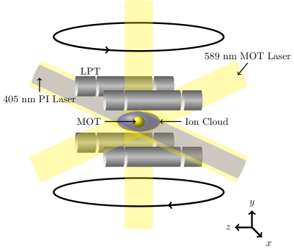
Figure 2: (Color online) A diagram of the hybrid apparatus used in these experiments. The anti-Helmholtz coils, with current directions shown by arrows, are located outside of the vacuum chamber (not shown).

The MOT can be characterized in two ways: using a photomultiplier tube (PMT) or using a CMOS camera. Both the PMT and the CMOS camera can be used to measure the trapped atom number, but the camera can also be used to measure the MOT radius. The MOT has a 1/$e$-density radius of $\approx 0.75$ mm and holds on the order of $10^{7}$ atoms. The PMT yields temporal information about the loading of the MOT.

The ions are created by a two-step process: atoms are resonantly excited to the 3P state by the trapping laser beams of the MOT, then they are ionized by a second laser beam at $405\,$nm. The first resonant step assures that the sample of loaded ions is pure, from the same species as the MOT neutrals.The beam size is fixed at a $1/e$-intensity radius of $1.8\,$mm, so the beam is always larger than the MOT and the intensity is approximately uniform over the size of the MOT. The photoionization intensity is controlled by changing the power of the $405\,$nm beam.

The LPT consists of four cylindrical segmented rods, each having three segments, that lie along the long edges of a square prism. The short segments at either end of the rods are known as the endcaps and provide axial confinement when DC voltages are applied to them. The length of these segments is $17.0$ mm. The longer central segment of the rod provides the radial confinement using r.f. voltages applied to the diagonal pairs of rods. The length of this segment is $2z_{0}=48.4\,$mm. The diagonal distance between the surfaces of the rods is $2r_{0}=19\,$mm and the vertical distance between the surface of the rods is $8.5\,$mm, to allow for access to the MOT cooling laser beams. The electrode radius is $r_{e}=8.8$ mm, giving a ratio $r_{e}/r_{0}=0.9$, slightly smaller than the ideal ratio of 1.1468 according to Ref. Denison (1971).

Our trap also deviates from the ideal Paul trapping potentials because the central segment is longer than the optimal length for a quadratic axial confining potential. Instead, the static axial confinement is a superposition of a quadratic and a quartic potential. As shown in our experiments and by the results of our simulations reported in Appendix B, trapping is possible even for electrode geometries that result in trapping potentials that have a strong quartic component and thus deviate considerably from the ideal quadrupole trapping potential. The price, as shown in Appendix B, is the emergence of deterministic chaos, even on the single-ion level, which reduces, and ultimately defines, the trapping volume of the LPT.

The number of ions in the Paul trap can be destructively measured using a channel electron multiplier (CEM). By putting DC voltages on the endcaps in a dipole configuration, the ions can be directed out of the trap along the axial direction toward the CEM. The programmed CEM extraction sequence captures a constant fraction of the number of ions trapped immediately before extraction. This extraction efficiency is built into our calibration Goodman et al. (2015), which thus allows us to determine the number of ions immediately before extraction. We use a custom LabVIEW virtual instrument (VI) to control the experimental timing and to record the measurements.

The basic experimental scheme is to allow the MOT to load to steady state from the background vapor in the presence of the photoionizing (PI) beam, then the ion trapping potentials are turned on. This way the loading rate from the MOT is constant during the entire time the ion trap is being loaded. The ions are extracted after a set delay time of $0.001$ s after the loading ends and the ion number is measured by the CEM during a $1$ s interrogation time. Since we can only measure the ion number destructively, we take many measurements at different loading times to create a time series of the ion number as a function of loading time.

It is impossible to completely remove the ion loss mechanisms of the LPT, so the loading rate can never be measured independently of the loss rate. Whatever the exact form of the differential equation for the loading of the LPT, the loss rate depends on the number of trapped ions and the loading rate is independent of the number of trapped ions. Therefore, to measure the loading rate, the ion number is measured for very short loading times ($\approx 0.05\,$s or shorter), where the loading can be described by [see (2)]

$$\frac{dN}{d\tau}\approx\Lambda.$$ (3)

An example of this is shown in Fig. 3. We see that in the limit of small loading times the number of ions trapped is a linear function of loading time.

Figure 3: (Color online) Ion signal as a function of time for short loading times, which minimizes the effects from losses. The ion signal is proportional to the number of trapped ions; the slope is the loading rate from the MOT. Where the error bars (showing statistical errors) are not seen, they are smaller than the corresponding plot symbols.

To measure the steady-state ion number, the loading time is set to be long enough to ensure that the ion population in the trap has reached equilibrium. At the lowest loading rates this time could be up to 3 minutes; at the highest loading rates the trap is saturated in milliseconds. Several consecutive measurements of the ion number are taken at a single loading time, then averaged to find the steady-state ion number. The loading rate is controlled by changing the $405\,$nm PI beam intensity and the process is repeated until the accessible part of the steady-state ion number as a function of loading rate is mapped out. With no PI beam present, no ion signal is measured.

The CEM measures a voltage that is proportional to the ion number, but the exact proportionality depends on the high-voltage gain applied to it. The most straightforward way to calibrate the CEM voltage would be to use an optical method to count the ion population and record the corresponding CEM voltage. However, because there are no optically accessible transitions in Na⁺, the number of ions could not be measured directly. Furthermore, our CEM is designed to have a large bias current, which allows it to detect large ion signals. Consequently, the CEM can only operate in an analog detection mode and cannot be calibrated using pulse counting methods like those used in Ref. Ravi et al. (2012b).

Instead, we used the same indirect method that we have used previously Goodman et al. (2015), which we will briefly describe here. The ion loading rate is measured two ways and then compared. First, the method described in Fig. 3 is used, with the assumption that the fraction of ions measured by the CEM, whatever it may be, does not change. The second method compares the loading of the MOT as a function of time with and without the PI beam present. The increase of the loss rate in the presence of the $405\,$nm beam is equivalent to the loading rate of the Paul trap, under the assumption that every ion created from the MOT is trapped. This assumption is good when the MOT is smaller than the trapping volume of the Paul trap. To convert the PMT voltage to units of number-of-atoms, we use the two-level atom model to determine the excited-state population of the type-II MOT. One would expect this approximation to be especially poor in the case of the type-II MOT, where multiple hyperfine levels in the excited state play a role in the pumping transition. We find however that the two-level model used with a modified saturation intensity of $37.6\,$mW/cm², compared to the theoretical saturation intensity of $13.4\,$mW/cm², fits quite well.

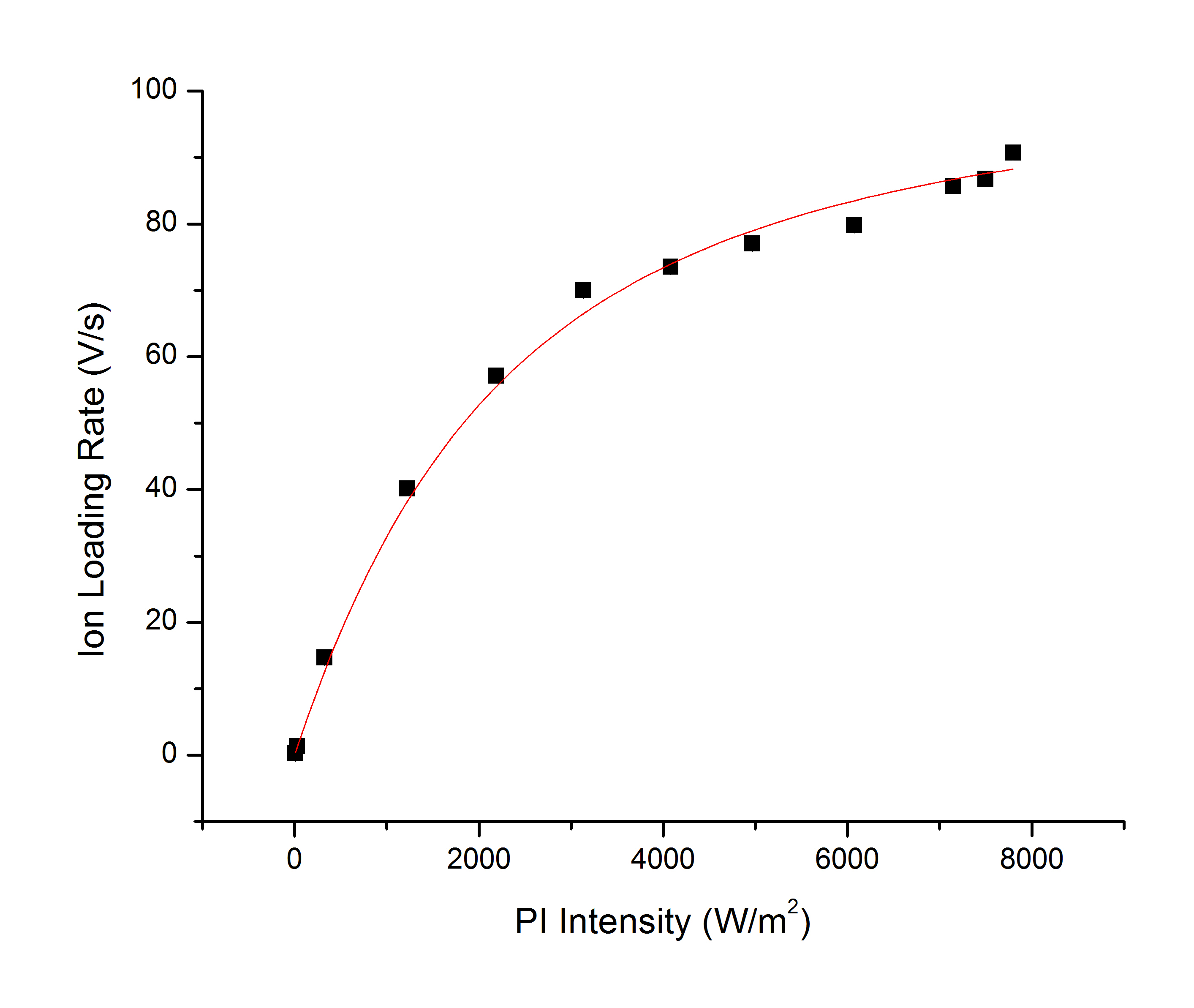
Figure 4: (Color online) Two-way measurement of the ion loading rate as a function of the intensity of the photo-ionizing laser for the purpose of finding the calibration factor between the ion signal and the number of ions. Measurements using the CEM (black squares) are compared to measurements of the atom loss rate from the MOT in the presence of the photoionization laser (solid red line) multiplied by a fitted scaling factor, which is the reciprocal of the CEM calibration factor. Where the error bars (showing statistical errors) are not seen, they are smaller than the corresponding plot symbols.

The two ion-loading rates are plotted and compared using a one-parameter fit, where the fitting parameter is the number of volts per ion. As seen in Fig. 4, the fit shows good agreement with the data for all CEM bias voltages. This justifies the assumptions required for the calibration.

III Experimental Results

As discussed in Sec. II, the electric potential in our LPT is not a pure, ideal quadrupole potential, but has a significant admixture of a quartic component. As discussed further in Appendix B, the quartic component in our potential leads to single-ion chaos, which renders our trap unstable in the radial direction from about $r=5\,$mm on, where $r=\sqrt{x^{2}+y^{2}}$ is the radial distance from the axis of the LPT. This might suggest that a proper description of our LPT is possible only in terms of a sum of quadratic and quartic terms. However, since up to $r=5\,$mm the quartic terms are small compared to the quadratic component, a simpler description of our LPT potential as a quadratic potential with a cut-off at $r=\hat{R}_{\rm cut}\approx 5\,$mm is possible. In this approximation, for $r<\hat{R}_{\rm cut}$, the electric potential of our LPT, written in SI units, is a pure quadrupole potential, given by Sivarajah et al. (2012); Goodman et al. (2012):

$$\phi(\vec{r},\tau)=V_{\rm rf}\cos(\Omega\tau)\left(\frac{x^{2}-y^{2}}{r_{0}^{2}}\right)+\frac{\eta V_{\rm end}}{z_{0}^{2}}(z^{2}-\frac{1}{2}x^{2}-\frac{1}{2}y^{2}),$$ (4)

where $\vec{r}=(x,y,z)$ is the position vector of an ion in the trap, $\tau$ is the time, $V_{\rm rf}$ is the rf voltage applied to the electrodes of the trap, $\Omega=2\pi f$ is the angular frequency of the applied rf voltage ($f$ is the lab frequency), $r_{0}$ and $z_{0}$ are defined in Sec. II, $\eta=0.3$ is a dimensionless efficiency parameter, and $V_{\rm end}$ is the voltage applied to the end-segments of the trap. For $r>\hat{R}_{\rm cut}$ the form of the potential is not needed, since ions are rapidly ejected from the trap (see Appendix B) as soon as they cross the chaos border at $r=\hat{R}_{\rm cut}$. Measured with respect to $\hat{R}_{\rm cut}$, and in pseudo-potential approximation (see Appendix A), the depth of the LPT potential is given by

$$D=\left[\frac{e^{2}V_{\rm rf}^{2}}{m\Omega^{2}r_{0}^{4}}-\frac{e\eta V_{\rm end}}{2z_{0}^{2}}\right]\,\hat{R}_{\rm cut}^{2}.$$ (5)

Experimentally, the trap depth $D$ can be changed by changing the rf amplitude $V_{\rm rf}$, the angular rf frequency $\Omega$ (via its dependence on the lab frequency $f=\Omega/(2\pi)$), or the end-cap potential $V_{\rm end}$. In the experiments reported in this paper, $V_{\rm end}=30\,$V is kept constant and only $V_{\rm rf}$ and $f$ are varied. Equation (5) was derived for a single trapped ion; if a second ion is trapped, the Coulomb repulsion changes the effective trap depth each ion experiences. The anti-trapping space-charge effect from multiple trapped ions makes the trap depth no longer expressible analytically. However, as supported by our analysis of ion numbers in the saturation region II below, the functional dependence of the trap depth on $V_{\rm rf}$ and $f$ appears to be the same.

It is convenient to express the trap depth in terms of the single-particle stability parameter

$$q=\frac{4eV_{\rm rf}}{m\Omega^{2}r_{0}^{2}}$$ (6)

so that

$$D=\left[\frac{qeV_{\rm rf}}{4r_{0}^{2}}-\frac{e\eta V_{\rm end}}{2z_{0}^{2}}\right]\,\hat{R}_{\rm cut}^{2}.$$ (7)

We also define the dimensionless loading rate

$$\lambda=2\pi\Lambda/\Omega,$$ (8)

i.e., the number of ions loaded per rf cycle.

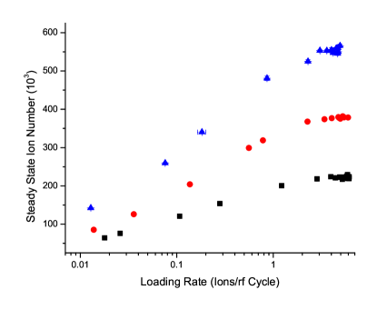
Figure 5: (Color online) Loading curves taken at constant $q=0.3$ and plotted on a lin-log scale. The trap settings were $V_{\mathrm{rf}}=13$ V and $f=450$ kHz for the squares (black), $V_{\mathrm{rf}}=16$ V and $f=500$ kHz for the circles (red), and $V_{\mathrm{rf}}=19.5$ V and $f=550$ kHz for the triangles (blue). Where the error bars (showing statistical errors) are not seen, they are smaller than the corresponding plot symbols.

In Fig. 5, loading curves of the steady-state ion number as a function of loading rate $\lambda$ are shown for three sets of rf parameters that each result in $q=0.3$. In each case, both the monotonic rise in region I and the plateau of region II are visible, predicted and previously observed in [21]. Since $q$ is kept constant in all three cases shown in Fig. 5, the depth of the LPT potential in these three cases is most conveniently evaluated according to (7). In addition, (7) shows that, for constant $q$, $D$ is independent of the frequency and depends only on $V_{\rm rf}$ and geometric constants of the LPT. Because of the quadratic form (4) of the LPT potential, the trapped ion cloud is an ellipsoid with semi-major axes equal to $\hat{R}_{\rm cut}$ in the $x$ and $y$ directions. In the $z$ direction we have $D=m\omega_{z}^{2}\hat{Z}_{\rm cut}^{2}$, where $\hat{Z}_{\rm cut}$ is the extent of the ion cloud in the $z$ direction and $\omega_{z}$ is the pseudo-oscillator frequency in the $z$ direction. Since $\omega_{z}$ is determined by the static potential due to the end-caps of the LPT, $\omega_{z}$ is a constant and, therefore, $\hat{Z}_{\rm cut}\sim\sqrt{D}$. Thus, the volume of the trapped ion cloud is $V=(4\pi/3)\hat{R}_{\rm cut}^{2}\hat{Z}_{\rm cut}\sim\hat{R}_{\rm cut}^{2}\sqrt{D}$. According to Poisson’s equation of electrostatics, the density $\rho$ of the trapped ions is proportional to the Laplacian of the trapping potential, i.e., according to (4), $\rho\sim\nabla^{2}\phi\sim V_{\rm rf}^{2}/\Omega^{2}$. This is all we need to predict, up to a proportionality constant, the number, $N$, of stored particles in the LPT. On the basis of the above discussion we have

$$N=\rho V\sim\hat{R}_{\rm cut}^{2}V_{\rm rf}^{2}D^{1/2}/\Omega^{2}.$$ (9)

More details on the derivation of (9) can be found in Sec. V.2.

We can now use (9) for a consistency check of our experimental results in Fig. 5. Denoting by $N_{13}$, $N_{16}$, and $N_{19.5}$, the particle numbers corresponding to the cases $V_{\rm rf}=13\,$V, $V_{\rm rf}=16\,$V, and $V_{\rm rf}=19.5\,$V, respectively, in their asymptotic regimes, we may take their ratios $N_{13}:N_{16}:N_{19.5}$, which we can predict on the basis of (9), even without knowledge of the proportionality constant in (9). Indeed, assuming that $\hat{R}_{\rm cut}$ depends only weakly on $V_{\rm rf}$ and $\Omega$, the cut-off radius $\hat{R}_{\rm cut}$ cancels when taking ion-number ratios on the basis of (9). Thus, the computation of ratios involves only $V_{\rm rf}$, $\Omega$, and known geometric constants. This way we obtain the explicit, analytical prediction $N_{13}:N_{16}:N_{19.5}=1:1.63:2.48$. This prediction may be compared with the actual ion numbers in the plateau regimes read off from Fig. 5. With $N_{13}\approx 225,000$, $N_{16}\approx 380,000$, and $N_{19.5}\approx 550,000$, we obtain $N_{13}:N_{16}:N_{19.5}=1:1.69:2.44$. This is in excellent agreement with the theoretical prediction. As mentioned above, taking ratios has the advantage of eliminating $\hat{R}_{\rm cut}$, which is difficult to obtain directly in our experiments, since the trapped Na⁺ ions are dark.

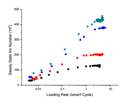
Figure 6: (Color online) Loading curves taken at constant $V_{\mathrm{rf}}=16$ V and plotted on a lin-log scale. The trap settings were $q=0.22$ and $f=580$ kHz for the squares (black), $q=0.26$ and $f=535$ kHz for the circles (red), $q=0.30$ and $f=500$ kHz for the upright triangles (blue), and $q=0.37$ and $f=450$ kHz for the inverted triangles (turquoise). The plots are in order of their trap depths. Where the error bars (showing statistical errors) are not seen, they are smaller than the corresponding plot symbols.

Region I and region II can likewise be seen in the curves shown in Fig. 6, which are taken at a constant rf amplitude, $V_{\rm rf}=16\,$V. Shown in Fig. 6 are four loading curves with $f=580\,$kHz, $535\,$kHz, $500\,$kHz, and $450\,$kHz. Using the frequencies as labels, we read off $N_{580}\approx 130,000$, $N_{535}\approx 200,000$, $N_{500}\approx 380,000$, and $N_{450}\approx 430,000$, which yield the ratios $N_{580}:N_{535}:N_{500}:N_{450}=1:1.54:2.92:3.31$. The theoretical prediction for these ratios, according to (9), is $N_{580}:N_{535}:N_{500}:N_{450}=1:1.57:2.14:3.29$. Just like for the results shown in Fig. 5, and except for the curve with $f=500\,$kHz, the experimental ratios match the theoretical predictions very well. At present it is not clear why the third curve, at $f=500\,$kHz, is an outlier in this sequence. This is the more puzzling that this curve is the same as the corresponding curve shown in Fig. 5, where it fits the sequence in Fig. 5 very well. That this curve does not fit well in Fig. 6 is also immediately obvious from the visual context in Fig. 6. This curve produces a gap in region II of Fig. 6, whereas a more even spacing was expected, mirroring the small decrements in frequencies corresponding to the four curves shown in Fig. 6.

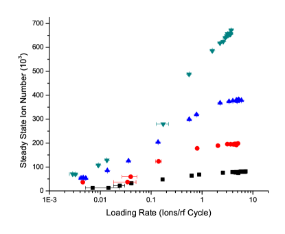
Figure 7: (Color online) Loading curves taken at constant $f=500$ kHz and plotted on a lin-log scale. The trap settings were $q=0.22$ and $V_{\mathrm{rf}}=12$ V for the squares (black), $q=0.26$ and $V_{\mathrm{rf}}=14$ V for the circles (red), $q=0.30$ and $V_{\mathrm{rf}}=16$ V for the upright triangles (blue), and $q=0.37$ and $V_{\mathrm{rf}}=20$ V for the inverted triangles (turquoise). The plots are in order of their trap depths. Where the error bars (showing statistical errors) are not seen, they are smaller than the corresponding plot symbols.

Several loading curves were also taken at a constant rf frequency; they are shown in Fig. 7. Akin to Figs. 5 and 6, the three lower curves all show both region I and region II. Only the loading curve taken at the largest rf voltage ($V_{\rm rf}=20\,$V) does not look like it has reached saturation (region II) yet, an impression confirmed by our ratio test to be conducted next. In the case of Fig. 7 there is a wrinkle in our theoretical analysis of the case $V_{\rm rf}=12\,$V in that for the experimental parameters the density (7) comes out negative, which means that we do not obtain a real square root in (9) and therefore $N$ cannot be predicted. This is not a disaster. It simply means that for $V_{\rm rf}=12\,$V and $f=500\,$kHz, our trap is operated so closely to the global instability border of the LPT that the pseudo-potential analysis (see Appendix A) is not accurate enough in this borderline case to make accurate predictions. For our ratio test we opted to ignore this case and normalize to the second curve in Fig. 7, i.e., the case $V_{\rm rf}=14\,$V, $f=500\,$kHz, for which we obtain a positive trap depth of substantial magnitude for which our pseudo-potential analysis is valid. Using voltages as labels, like we did in the case of Fig. 5, we predict $N_{14}:N_{16}:N_{20}=1:1.95:4.65$. From Fig. 7 we read off $N_{14}\approx 190,000$, $N_{16}\approx 380,000$, and $N_{20}\approx 660,000$, which results in the experimental ratios $N_{14}:N_{16}:N_{20}=1:2.00:3.47$. Similarly to the cases discussed in connection with Figs. 5 and 6, the ion-number ratio of the two cases of Fig. 7, which are confidently in region II, is very close to its predicted value. In contrast, the predicted ratio for $N_{20}/N_{14}$ is much larger than the experimentally observed ratio, confirming our suspicion that for $V_{\rm rf}=20\,$V and at $\lambda=3\,$ions/rf-cycle the loading curve in this case is still climbing (still in region I), and its saturated ion number, expected to occur at higher values of $\lambda$ than those shown in Fig. 7, will eventually be larger than $N=660,000$.

The question arises whether we may simplify the expression (5) [(7), respectively] for the density $D$, perhaps by neglecting the term proportional to $V_{\rm end}$, in order to turn (9) into a more concise formula. Alas, as the case $V_{\rm rf}=12\,$V in Fig. 7 vividly illustrates, this is not possible. The two terms, i.e., the terms involving $V_{\rm rf}$ and $V_{\rm end}$ in (5) [(7), respectively], are of similar magnitude, which makes it impossible to neglect one with respect to the other. Thus, the square-root behavior in (9) is essential.

Our theoretical estimates and predictions above are based on a single-ion picture (the pseudo-potential analysis presented in Appendix A), and do not include any space-charge- or many-body effects. The overall excellent agreement of our predictions for the ion-number ratios in region II of the cases shown in Figs. 5, 6, and 7 leads us to conclude that in our LPT experiments these effects are either negligible or lead to a simple renormalization of our expression for $N$ that results in an overall constant that cancels upon taking ratios. In Sec. V.2, based on the single-particle pseudo-potential picture, we make predictions of the absolute magnitude of $N$ in region II, which agree very well with the experimentally observed values. This might argue for the space-charge- and many-body effects to be negligible. However, since $\hat{R}_{\rm cut}$ enters these formulas multiplicatively, we cannot be sure whether the renormalization constant is not simply absorbed in our effective $\hat{R}_{\rm cut}$, used in Sec. V.2. Only direct experimental observation of $\hat{R}_{\rm cut}$ can resolve this issue. This, however, due to the optical darkness of the Na⁺ ions used in our experiments, is currently beyond our experimental capabilities. Nevertheless, the excellent agreement of the experimental ion-number ratios in region II with our theoretical predictions supports the validity of our experimental LPT ion-loading curves.

IV Simulations

Model simulations have already been done Blümel et al. (2015) that confirm the existence of the four different dynamical regimes. In addition it was shown in Blümel et al. (2015) that the phenomenon is robust with respect to the statistical distribution of time between loading events, temperature, loading mechanisms, and the geometry of the absorbing boundary. So here the emphasis is not so much on proving the existence of the four dynamical regions, or their robustness, but to see whether the simulations can qualitatively, and to some extent quantitatively, describe the experimentally observed characteristics of regions I and II.

Since independence of the loading statistics has already been demonstrated in Blümel et al. (2015), we focus in this paper on the case of uniform loading statistics. Qualitatively, our results stay valid, which we checked explicitly, if different loading statistics, such as Gaussian statistics, are used.

The Newtonian equations of motion of a singly charged ion of mass $m$ in the trap is

$$m\frac{d^{2}\vec{r}}{d\tau^{2}}=-e\vec{\nabla}\phi(\vec{r},\tau),$$ (10)

which, written out in components, results in

$$m\frac{d^{2}}{d\tau^{2}}\left(\begin{matrix}x\cr y\cr z\cr\end{matrix}\right)=\left(\begin{matrix}-2V_{\rm rf}e\cos(\Omega\tau)\frac{x}{r_{0}^{2}}+\frac{\eta eV_{\rm end}}{z_{0}^{2}}x\cr 2V_{\rm rf}e\cos(\Omega\tau)\frac{y}{r_{0}^{2}}+\frac{\eta eV_{\rm end}}{z_{0}^{2}}y\cr-\frac{2\eta eV_{\rm end}}{z_{0}^{2}}z\cr\end{matrix}\right).$$ (11)

Defining the dimensionless time

$$t=\left(\frac{\Omega}{2}\right)\tau,$$ (12)

the set of equations may be written as

$$\left(\begin{matrix}\ddot{x}\cr\ddot{y}\cr\ddot{z}\cr\end{matrix}\right)=\left(\begin{matrix}-2q\cos(2t)x+bx\cr 2q\cos(2t)y+by\cr-2bz\cr\end{matrix}\right),$$ (13)

where the dots indicate differentiation with respect to dimensionless time $t$, the dimensionless control parameter $q$ is defined in (6), and

$$b=\frac{4e\eta V_{\rm end}}{m\Omega^{2}z_{0}^{2}}.$$ (14)

If more than one ion of charge $e$ and mass $m$ are stored in the trap, the ions interact via the Coulomb force, resulting in the following set of coupled equations:

$$\left(\begin{matrix}\ddot{x}_{i}+2q\cos(2t)x_{i}-bx_{i}\cr\ddot{y}_{i}-2q\cos(2t)y_{i}-by_{i}\cr\ddot{z}_{i}+2bz_{i}\cr\end{matrix}\right)=\sum_{\begin{subarray}{c}j=1\\ j\neq i\end{subarray}}^{N}\frac{\vec{r}_{i}-\vec{r}_{j}}{|\vec{r}_{i}-\vec{r}_{j}|^{3}},$$ (15)

where $i=1,\ldots,N$ counts the number of particles in the trap at time $t$, and $\vec{r}$ is measured in units of

$$l_{0}=\left(\frac{e^{2}}{\pi\epsilon_{0}m\Omega^{2}}\right)^{1/3},$$ (16)

where $\epsilon_{0}$ is the electric permittivity of the vacuum.

It is the introduction of the unit of length (16) that allows us to normalize the coefficient in front of the Coulomb force on the right-hand side of (15) to 1, and thus arrive at the set of equations (15) that depends only on the two dimensionless parameters $q$ and $b$. $q$ is an adjustable control parameter that, depending on the trap voltage $V_{\mathrm{rf}}$ and frequency $f$, may be set to a value in the interval $0<q\lesssim 0.9$, where $q\approx 0.9$ is the Mathieu instability limit Abramowitz and Stegun (1964). It is shown in Appendix A that for given $q$, in order to achieve trapping, the parameter $b$ has to satisfy $0<b<q^{2}/2$.

Numerically, because of the repulsive Coulomb interactions in (15), and even for a large number $N$ of trapped ions, the coupled set of equations (15) is well conditioned. Therefore, a standard 4th order Runge-Kutta method Press et al. (1992) is enough to reliably integrate (15).

While our numerical model (15) captures the essence of the experimental LPT, and its parameters $q$ and $b$ are adjusted to their experimental values, our model is nevertheless an idealization. The electrodes in our experiment are not hyperbolic surfaces, as required if (15) is expected to be exact, and while (15) assumes a quadratic potential in $z$ direction, the potential in our LPT also has a quartic component Goodman et al. (2012); Sivarajah et al. (2012). Still, the proportions of the numerical trap, as expressed in (15), are correct and we expect that our model captures the essential parts of the physics in our experimental LPT.

A final comment concerns the number of particles we are able to simulate compared with the number of particles in our experimental trap. In order to accumulate sufficient statistics, and given our computer resources, we found that 2,000 simultaneously stored ions are a practical upper limit for our numerical simulations. Although orders of magnitude smaller than the experimental number of particles in our trap, 2,000 particles is not a small number, and using scaling relations, to be discussed below, we are able to compare our simulations not just qualitatively, but also quantitatively with our experimental results.

Our simulations proceed in the following way. For a given loading rate $\lambda$ we generate a time sequence $t_{j},j=1,...,M$ of loading events, which have a Poissonian distribution whose average corresponds to the specified loading rate $\lambda$. For each individual parameter setting we check that $M$ is large enough so that we are deeply in the saturated regime where we are able to extract the steady-state number of ions, $N_{s}$, with excellent statistics. Denoting by $\langle\ldots\rangle_{t}$ the time average in the saturated regime, we also compute the statistical spread $\Delta N_{s}=\sqrt{\langle N_{s}^{2}\rangle_{t}-\langle N_{s}\rangle_{t}^{2}}$, which characterizes the ion-number fluctuations in the saturated regime due to the Poissonian loading process. At each loading event $t_{j}$ a new ion with zero initial velocity is created in the trap at a random location inside of a spherical loading zone of radius $\hat{R}_{\rm load}$ (in SI units), representing the creation of ions from the MOT via the photoionizing $405\,$nm laser. Between loading events, i.e. for $t$ in $t_{j}<t<t_{j+1}$, we integrate the ion trajectories in the trap, including the newly created ion, according to the system (15). Once $t_{j+1}$ is reached, we eliminate all ions from the trap whose positions at $t_{j+1}$ lie beyond a pre-specified absorbing boundary B. In Blümel et al. (2015) we already showed that the qualitative shape of the $N_{s}(\lambda)$ curves does not depend on the geometry of B. Therefore, making use of this freedom, we chose in this paper a cylindrical absorbing boundary B with radius $\hat{R}_{\rm cut}$ in the $x$-$y$ direction and total length $2z_{0}$ in the $z$ direction, i.e., ions are absorbed in the $z$ direction if they exceed $|z|=\hat{Z}_{\rm cut}=z_{0}=24.2\,$mm.

In addition to $q$, all we need for our simulations are the parameters $b$, $R_{\rm load}=\hat{R}_{\rm load}/l_{0}$, $R_{\rm cut}=\hat{R}_{\rm cut}/l_{0}$, and $Z_{\rm cut}=\hat{Z}_{\rm cut}/l_{0}$. The radius of the loading zone $\hat{R}_{\rm load}$ is defined by the size of the type-II MOT, which, according to Ref. Goodman et al. (2015), is $r_{a}=0.75\,$mm. The electrodes are positioned at $r_{0}=9.5\,$mm, which is the upper bound for $\hat{R}_{\mathrm{cut}}$. According to the discussion above, we cannot simulate the full-sized experimental LPT, since it typically holds more ions than we are able to realistically simulate. Accordingly, we simulate a scaled-down version of our LPT in which all linear dimensions are scaled by a factor $0<\sigma<1$, resulting in

$$R_{\rm load} =\sigma\hat{R}_{\rm load}/l_{0}=88.4\,\sigma\,[f({\rm MHz})]^{2/3},$$ (17)

$$R_{\rm cut} =\sigma\hat{R}_{\rm cut}/l_{0}=1119.1\,\sigma\,[f({\rm MHz})]^{2/3},$$ (18)

$$Z_{\rm cut} =\sigma\hat{Z}_{\rm cut}/l_{0}=2827.2\,\sigma\,[f({\rm MHz})]^{2/3}.$$ (19)

As discussed in Sec. III, in a harmonic trap, i.e., a trap with time-independent quadratic trapping potentials in all three directions, and at zero temperature, the charge density $\rho_{\rm el}$ in the trap is constant, which follows immediately from $\rho_{\rm el}\sim\nabla^{2}\phi$. In this case the particle number in the trap scales with the volume of the trap, i.e.,

$$N\sim\sigma^{3}.$$ (20)

Although our experimental trap is not exactly harmonic, and the temperature is finite, we nevertheless expect that (20) holds to a good approximation. Therefore, in order to compare with our experimental results, we scale $N_{s}$ obtained from our simulations according to

$$N_{s}^{\rm scaled}=N_{s}^{\rm simulated}/\sigma^{3},$$ (21)

which allows a direct comparison between the results of our simulations with experimental results of the saturated number of ions in the trap.

We are now ready for the numerical simulations. Since they are expensive, we focused on simulating the constant-$q$ experiments, performed with $q=0.3$, and described in Sec. III. Figure 8 shows the results of our simulations.

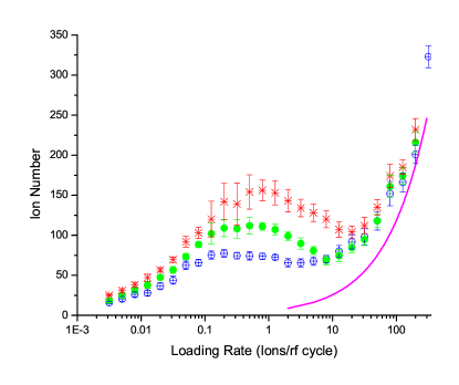
Figure 8: (Color online) Simulation results for the model LPT performed at constant $q=0.3$ for three different combinations of rf voltage and frequencies. $f=450\,$kHz, $V=13\,$V: open, blue circles; $f=500\,$kHz, $V=16\,$V: filled, green circles; $f=550\,$kHz, $V=19.5\,$V: red asterisks. Scale parameter: $\sigma=1/40$. These simulation results may be compared with the three corresponding LPT experiments shown in Fig. 5. The heavy solid line (purple) is the analytical result for $N_{s}(\lambda)$ in region IV Blümel et al. (2015). The lengths of the error bars, equal to $2\Delta N_{s}$, characterize the statistical fluctuations of the ion number in the saturated regime.

Compared with the experimental results shown in Fig. 5 we see that in our simulations the maximum of region II occurs at a loading rate which is about a factor 10 lower than in the experiments. However, the location of the region-II maximum depends on the scaling factor $\sigma$ and shifts to higher loading rates as $\sigma$ approaches 1 where the simulated ion trap size becomes identical to the experimental Paul trap. This effect can be seen in Fig. 9, where simulations are plotted at several different values of $\sigma$, along with several experimental curves. Additionally, the simulations in Fig. 9 have been scaled up in ion number [see (21)]. The simulated ion curves match the experiments in the ion number, but the regions occur at different ion loading rates. The reason for this discrepancy is not clear. It is possible that effects not included in the idealizations made for the simulations, such as stray fields causing excess micromotion or the presence of the grounded vacuum chamber, are the cause.

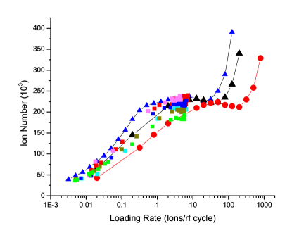
Figure 9: (Color online) Simulations of loading curves at three scaling factors: $\sigma=1/10$ small triangles (blue), $\sigma=1/8$ large triangles (black), and $\sigma=1/5$ circles (red). Also shown are a number of experimental loading curves (squares) at $q=0.30$, $V_{\mathrm{rf}}=13$ V, and $f=450$ kHz. The scatter of the experimental data points gives an idea of the statistical and systematic variations in our experimental loading data. For these simulations, $\hat{R}_{\rm cut}=4.5\,$mm was chosen, which, as a result of many simulations, akin to those shown in this figure, turned out to yield the best agreement with the experimental results. Where the experimental error bars (showing statistical errors) are not seen, they are smaller than the corresponding plot symbols.

V Analytical Theory

In this section we present an analytical theory for regions I and II. In Sec. V.A we show that in region I the saturated ion number $N_{s}(\lambda)$ follows a power law in $\lambda$, which we confirm experimentally. We also compute the approximate exponent of the power law, which agrees well with our experiments. In Sec. V.B we present a theory for region II. This theory explains the plateau behavior of $N_{s}(\lambda)$ in region II and also fits the temporal behavior of $N_{s}(\lambda,t)$ better than all other theories so far described in the literature.

V.1 Region I

In this subsection we present a simple, analytically solvable model for the steady-state ion population $N_{s}(\lambda)$ as a function of loading rate $\lambda$. Our model predicts monotonic power law behavior in region I. Under certain reasonable assumptions, based on heating rates obtained from molecular-dynamics simulations of non-neutral plasmas published in the literature Tarnas et al. (2013), the exponent derived from our analytical model is close to the exponent observed in our experiments. Since our analytical calculations assume spherical symmetry, our analytical results for region I are primarily applicable to the three-dimensional quadrupole Paul trap (3DPT). Comparing with experiment, we found that these results also hold well for the LPT.

In region I we need to consider the stationary state in which for each particle loaded one particle escapes. In the stationary state the spatial probability distribution, $\rho(\vec{r}\,)$, of the ions in the trap is approximately Gaussian with a width that is proportional to $\sqrt{T}$, where $T$ is the temperature. Since, according to $E\sim kT$, where $k$ is the Boltzmann constant, the average energy $E$ of a stored ion is proportional to $T$, the width of the spatial Gaussian is proportional to $\sqrt{E}$.

In order to obtain analytical results in closed form, we replace the Gaussian distribution by a flat distribution with a sharp cut-off, i.e. we represent the spatial density $\rho(\vec{r}\,)$ by a homogeneous sphere according to

$$\rho(\vec{r}\,)=\begin{cases}\displaystyle\frac{3N_{s}}{4\pi w^{3}},&|\vec{r}\,|\leq w,\\ 0,&|\vec{r}\,|>w,\end{cases}$$ (22)

where $N_{s}$ is the number of ions in steady state,

$$w=\alpha\sqrt{E}$$ (23)

is the radial width of the density distribution, and $\alpha$ is a constant. Since a Gaussian is a steeply descending function in the wings, the approximation (22) is benign and does not change the scaling of $N_{s}(\lambda)$ in $\lambda$.

We start with the situation in which the probability sphere, due to rf heating Tarnas et al. (2013); Nam et al. (2014); Blümel et al. (1988), has expanded beyond the location $R_{\rm cut}$ of the absorbing boundary B, just far enough for the total excess probability beyond $R_{\rm cut}$ to integrate to 1 particle. Denote by $\kappa$ the heating rate per particle. Then, the energy $E$ per particle is

$$E=E_{0}+\kappa\Delta\tau,$$ (24)

where $\Delta\tau$ is the time that has passed since the last loading (ion creation) event and $E_{0}$ is the energy per particle immediately after the last loading event. Since we are in the steady state, exactly $\Delta\tau=1/\Lambda$ has passed on average between ion creation and ion loss, where $\Lambda$ is the loading rate. Therefore, from (24),

$$E=E_{0}+\frac{\kappa}{\Lambda},$$ (25)

and, according to (23),

$$w=\alpha\left(E_{0}+\frac{\kappa}{\Lambda}\right)^{1/2}.$$ (26)

The excess width is

$$\delta w=w-R_{\rm cut}=\alpha\left(E_{0}+\frac{\kappa}{\Lambda}\right)^{1/2}-R_{\rm cut}.$$ (27)

In steady state, the excess width $\delta w$ corresponds to exactly 1 particle. Therefore, denoting by $\delta V$ the volume of the shell of width $\delta w$:

$$1 =\rho\delta V=\rho 4\pi R_{\rm cut}^{2}\delta w$$

$$=\left(\frac{3N_{s}}{4\pi R_{\rm cut}^{3}}\right)4\pi R_{\rm cut}^{2}\left[\alpha\left(E_{0}+\frac{\kappa}{\Lambda}\right)^{1/2}-R_{\rm cut}\right]$$

$$=\frac{3N_{s}}{R_{\rm cut}}\left[\alpha\left(E_{0}+\frac{\kappa}{\Lambda}\right)^{1/2}-R_{\rm cut}\right].$$ (28)

In region I, i.e., for small $\Lambda$, the dominant term in (28) is $\kappa/\Lambda$. Therefore, in region I, we may approximately write:

$$1=\frac{3N_{s}\alpha}{R_{\rm cut}}\left(\frac{\kappa}{\Lambda}\right)^{1/2}.$$ (29)

In order to compute the dependence of $N_{s}$ on $\Lambda$, we need to know how the heating rate $\kappa$ depends on $N_{s}$. In order to answer this question we turn to Fig. 2 of Tarnas et al. (2013). This figure shows the heating rate $H$ of $N$-ion clouds in steady state as a function of cloud size $\hat{s}$. This figure is relevant since, up to the choice of units, $\kappa$ and $H$ are identical. Therefore, the $N$-scaling of $\kappa$ is the same as the $N$-scaling of $H$. Although Fig. 2 of Ref. Tarnas et al. (2013) was computed for a 3DPT, it nevertheless gives us a first idea on the $N_{s}$ scaling of $\kappa$ for the LPT that we focus on in this paper. Since our trap has an effective radius $R_{\rm cut}$, we need to extract heating rates $H$ from Fig. 2 of Tarnas et al. (2013) as a function of $N$ at constant cloud size $\hat{s}$. The most striking feature of the heating data shown in Fig. 2 of Tarnas et al. (2013) is that the heating rate curves for different $N$ are parallel to each other and have about the same spacing when doubling the number of particles $N$. Therefore, since Fig. 2 of Tarnas et al. (2013) shows $H$ on a log scale, both features combined show that, at given $\hat{s}$, independently of $\hat{s}$, $H$ follows a power law in $N$. On the basis of the data displayed in Fig. 2 of Tarnas et al. (2013), we find, at constant $\hat{s}$:

$$H\sim N^{10/3}.$$ (30)

Therefore, because of $\kappa\sim H$, we obtain:

$$\kappa=\beta N_{s}^{10/3},$$ (31)

where $\beta$ is a constant. Using this result in (29), we obtain

$$1=\frac{3\alpha\beta^{1/2}N_{s}^{8/3}}{R_{\rm cut}\Lambda^{1/2}}.$$ (32)

Using (8), we solve (32) for $N_{s}$ in terms of $\lambda$:

$$N_{s}=\left[\frac{R_{\rm cut}}{3\alpha(2\pi\beta/\Omega)^{1/2}}\right]^{3/8}\ \lambda^{3/16}.$$ (33)

Thus, this simple model predicts $N_{s}\sim\lambda^{0.188}$, which may be compared with the experimental region-I result $N_{s}\sim\lambda^{0.281}$. Since the numerical value of the exponent predicted by our model depends on the scaling of the heating rate $\kappa$ in $N$, which was not separately determined for our LPT, the value of the exponent predicted by (33) is less important than the prediction that $N_{s}$ follows a power law. Therefore, we treat the value of the exponent as a fit parameter. Fits of the data from Fig. 5 using this model can be seen in Fig 10. The difference in the value of the exponent is likely due to the difference in heating rate between the ideal 3DPT of Tarnas et al. (2013) and the heating rate in the experimental LPT.

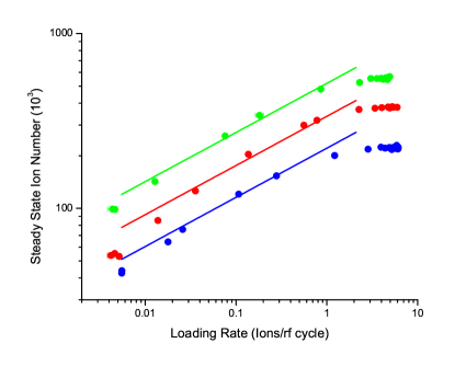
Figure 10: (Color online) The data points from Fig. 5 shown with fit using $N_{s}=A\lambda^{0.281}$. We see that the power-law form of the fit function, as predicted by our analytical model, fits the data in region I very well. Where the error bars (showing statistical errors) are not seen, they are smaller than the corresponding plot symbols.

Since rf heating is one of the central ingredients in this model, both the prediction of a power law in itself and the approximate agreement of the power law exponent with our experimental results indicate that rf heating is the factor that governs the behavior of $N_{s}(\lambda)$ in region I. This is corroborated by Fig. 11, which shows a comparison between $N_{s}$ obtained as a result of solving the fully time-dependent set of equations of motion (15), i.e., the equations of motion including rf heating (asterisks in Fig. 11) and $N_{s}$ obtained as a result of solving the time-independent pseudo-oscillator equations of motion (52), which, due to the lack of explicit time-dependence, are not capable of simulating rf heating (filled circles in Fig. 11). Clearly, while the pseudo-oscillator model is capable of reproducing regions II, III, and IV, it completely fails to reproduce region I, which can only be attributed to a lack of rf heating in the pseudo-oscillator model, since otherwise this model contains all many-body forces exactly as in the full set of equations (15). Thus, we proved conclusively that it is rf heating that determines both the power law and the power law’s exponent in region I.

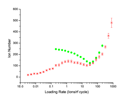
Figure 11: (Color online) Simulation of the LPT: Comparison between the time-dependent model with rf switched on (asterisks) and the pseudo-potential model with only the pseudo-potential present (filled circles). We simulated the case $V_{\rm rf}=16\,$V, $f=450\,$kHz, with scaling factor $\sigma=1/40$. The lengths of the error bars, equal to $2\Delta N_{s}$, characterize the statistical fluctuations of the ion number in the saturated regime. Where error bars are not seen, they are smaller than the plot symbols.

V.2 Region II

In region II, the steady-state ion number plateau is determined by the depth of the trap. The pseudopotential approximation, described in Appendix A, is valid in region II. The pseudopotential well is completely filled with ions in this region. The expression for the depth of the pseudopotential predicts a steady-state ion number in region II of

$$N_{s}^{II}=\frac{4\pi^{3}\epsilon_{0}m\times 10^{3}}{3e^{2}}f[\mathrm{Mhz}]^{2}\times\\ \hat{R}_{\rm cut}[\mathrm{mm}]^{3}q^{2}\sqrt{\frac{q^{2}}{4b}-\frac{1}{2}}.$$ (34)

There are no adjustable parameters in this expression. However, $\hat{R}_{\mathrm{cut}}$ is not easily determined for dark ions. The traditional derivations of the pseudopotential depth assume that $\hat{R}_{\mathrm{cut}}=r_{0}$ and that the ions are only lost when they collide with or move beyond the trap electrodes Ghosh (1995); Major et al. (2005). This has been shown not to be the case in recent hybrid trap work Ravi et al. (2012a); Goodman et al. (2015). Finding $\hat{R}_{\mathrm{cut}}$ directly allows the trap depth to be calculated without making any approximations. In principle, $\hat{R}_{\rm cut}$ can be found in a variety of ways.

The first is to follow the method used in Ravi et al. (2012a); Goodman et al. (2015), where the idealized single-particle trap depth is equated to the energy of a simple harmonic oscillator with spring constant $k=m\omega^{2}$, where $\omega$ is the secular frequency of the ionic motion. This method has the advantage of being simple, but the drawback is that it relies on the single-particle trap depth, which is a credible approximation, but may not be accurate enough. Indeed, this simple model disagreed with subsequent hybrid trap experiments, described in Goodman et al. (2015), by 25%.

A second method, mentioned in the caption of Fig. 9, is to find the $\hat{R}_{\mathrm{cut}}$ value which makes the simulations best match the experimental results. This requires some computationally demanding simulations of the trapped ions.

A third method is to find an $\hat{R}_{\mathrm{cut}}$ that makes (34) fit best at one trap setting. For sodium ions, (34) becomes

$$N_{s}^{II}=548344f[\mathrm{Mhz}]^{2}\hat{R}_{\mathrm{cut}}[\mathrm{mm}]^{3}q^{2}\sqrt{\frac{q^{2}}{4b}-\frac{1}{2}}.$$ (35)

By selecting a single data set and finding the $\hat{R}_{\mathrm{cut}}$ that makes both sides of (35) approximately equal, we are able to fit nearly all of our data at least as well as the other methods, and in some cases much better, using a much simpler procedure (see Table 1). The data set with the smallest ion number, which was taken at $q=0.22$, $V_{\mathrm{rf}}=16$ V, and $f=500$ kHz, is the one exception; using these parameters in this model returns an imaginary number of ions. These settings also have the smallest number of ions at steady state in region II, i.e., approximately 80000, which is still a large number for most Paul trap experiments. It is also unclear what differentiates the settings where this value of $\hat{R}_{\mathrm{cut}}$ fits well and the ones that do not.

There has been no previous study of why $\hat{R}_{\mathrm{cut}}\neq r_{0}$, but it has been hypothesized that it could be due to contributions from higher-order multipoles Alheit et al. (1996). In this paper we confirm that it is the admixture of the quartic component of the confining potential in $z$ direction that is responsible for the reduction of $\hat{R}_{\rm cut}$ to $\hat{R}_{\rm cut}<r_{0}$. In fact, while a single ion in an ideal trap, i.e., a trap in which only quadrupole potentials are present, is never chaotic, even when driven by the rf trap fields, a single ion in a potential with a quartic admixture shows a transition in space from regular, confined motion, to chaotic, unconfined motion (see Appendix B). This brings us to a fourth method for determining $\hat{R}_{\rm cut}$, described in detail in Appendix B. According to this method, $\hat{R}_{\rm cut}$ is identical with the single-ion chaos border. This means that for $r<\hat{R}_{\rm cut}$ the ion’s motion is perfectly regular and the ion, in the absence of noise, is perfectly trapped. However, as soon as $r$ exceeds $\hat{R}_{\rm cut}$, the ion’s motion becomes chaotic. As a consequence, the ion is free to explore spatial regions with $r>\hat{R}_{\rm cut}$, which quickly leads to an encounter with the electrodes at which the ion is absorbed. Thus, $\hat{R}_{\rm cut}$ is determined by a method that is based on the dynamics of a single ion and therefore allows a very quick and efficient determination of $\hat{R}_{\rm cut}$ for various trap settings. This method does not only have technical advantages for the determination of the value of $\hat{R}_{\rm cut}$. It also solves the puzzle of the very existence of $\hat{R}_{\rm cut}$, identifying its origin as a fundamental, purely dynamical effect, a chaos transition, whose exact location is determined by the strength of the admixture of higher multipole fields to the LPT’s quadrupole trapping field.

Table 1: The experimental ion number compared with the ion number predicted by (35) with $\hat{R}_{\mathrm{cut}}=3.74$ mm. The cells with N/A indicate an imaginary number predicted.

$q$	f[MHz]	$b$	Predicted Ion Number	Measured Ion Number	Percent Difference
0.30	0.550	0.022	574273	566162	1.4
0.30	0.500	0.026	387308	381897	1.4
0.30	0.450	0.032	231851	229396	1.1
0.22	0.500	0.026	N/A	81654	N/A
0.26	0.500	0.026	185254	198434	6.6
0.37	0.500	0.026	882666	672169	31.3
0.37	0.450	0.032	594951	455767	30.5
0.26	0.535	0.023	271704	205591	32.2
0.22	0.580	0.019	163397	132166	23.6

The loading of the Paul trap as a function of time was also examined. In our previous work Blümel et al. (2015), the loading as a function of time in region IV was determined from the equation

$$t=-\frac{2\tilde{R}}{3\tilde{\lambda}^{1/3}}\left\{\ln{(\alpha-\tilde{N}^{1/2}})-\frac{1}{2}\ln{(\tilde{N}+\alpha\tilde{N}^{1/2}+\alpha^{2})}\right.\\ \left.+\sqrt{3}\arctan{\left(\frac{2\tilde{N}^{1/2}+\alpha}{\alpha\sqrt{3}}\right)}-\sqrt{3}\arctan{\left(\frac{1}{\sqrt{3}}\right)}\right\},$$ (36)

where $\alpha=\tilde{R}^{1/2}\tilde{\lambda}^{1/3}$, and the tilde indicates that the quantity corresponds to the loading zone, which in this case is the MOT volume. Therefore, for example, $\tilde{R}$ is the radius of the loading zone, which in this case is the MOT radius.

Equation (36) was derived for region IV and one should not expect it to fit in regions I and II. Indeed, applying it to plots at extremely small loading rates results in poor fits and the prediction of imaginary ion numbers. However, in region II, (36) fits the loading data at least as well, if not better, than the traditional model (2). This includes versions of the traditional model where $\ell_{1}=0$ or $\ell_{2}=0$, as can be seen in Fig. 12. All forms of the traditional model demonstrate the overshoot of the rise, undershoot of the knee, and overshoot of the plateau seen also in Fig. 1. While (36) overshoots the rise as well, it fits the knee and the plateau better than the traditional model. Further, unlike the traditional model, it is derived from the underlying physical process and depends on quantities that can be experimentally measured independently of the model itself.

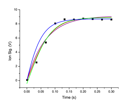
Figure 12: (Color Online) Ion number vs. time fitted to the model (36) (blue), the traditional model (2) (green), that model with $\ell_{2}=0$ (purple), and that model with $\ell_{1}=0$ (red). The traditional model displays the familiar overshoot-undershoot-overshoot pattern, but the model (36) fits both the knee and the plateau. Where the error bars (showing statistical errors) are not seen, they are smaller than the corresponding plot symbols.

VI Conclusion

In this work, two of the four regions in the loading curve of a Paul trap, predicted in Blümel et al. (2015), have been confirmed experimentally. Additionally, both simulations and analytical models match reasonably well to the steady-state ion number and shape of the curves. The two regions are relevant and accessible to the majority of Paul trap experiments. Also proposed are new, experimental and computational methods for finding $\hat{R}_{\mathrm{cut}}$, a quantity necessary for finding the actual trap depth (a difficult experimental prospect), the total collision rate constant for dark ions Lee et al. (2013); Goodman et al. (2015), and for describing the behavior of the Paul-trap loading in region III Blümel et al. (2015). Further work remains to be done to fully understand the loading of the Paul trap. An upcoming paper will examine the behavior of regions III and IV through experiment, simulations, and analytical theory.

VII Acknowledgements

W.W.S. would like to acknowledge NSF support (in part) from grant 1307874.

Appendix A: LPT Pseudopotential

In this appendix we derive the single-particle pseudopotential for the LPT used in the analysis of our experiments. The pseudopotential is used in our numerical simulations to prove (a) that the power-law behavior of the loading curves in region I is a consequence of rf heating, which we prove in reverse by demonstrating that the pseudo-potential equations of motion, lacking an rf term, cannot explain region I, and (b) that the existence of region II does not depend on the time-dependence of the rf drive of the trap, i.e., as demonstrated in Sec. V.2, the time-independent pseudopotential alone is capable of explaining the plateau in region II.

We start with the equations of motion (13), where $x$, $y$, and $z$ are in units of $l_{0}$ [see (16)], $t$ is in units of $2/\Omega$ [see (12)], and $q$, $b$ are the dimensionless control parameters defined in (6) and (14), respectively. Focusing on the $x$ component of (13), and following the procedure outlined in Landau and Lifshitz (2007), we split the $x$ coordinate into a large-amplitude, slowly varying component $X(t)$, called the macromotion, and a small-amplitude, fast-oscillating component $\xi(t)$, called the micromotion according to

$$x(t)=X(t)+\xi(t).$$ (37)

Defining the cycle average

$$\langle f(t)\rangle=\frac{1}{\pi}\int_{-\pi/2}^{\pi/2}f(t+t^{\prime})\,dt^{\prime},$$ (38)

and in line with the physical meanings of $X$ and $\xi$, we assume

$$\langle X(t)\rangle =X(t),\ \ \ \langle\xi(t)\rangle=0,$$

$$\langle\ddot{X}(t)\rangle =\ddot{X}(t),\ \ \ \langle\ddot{\xi}(t)\rangle=0.$$ (39)

Focusing first on the time-dependent (rf) part of (13) and using the decomposition (37), we have

$$\ddot{X}(t)+\ddot{\xi}(t)=-2q\cos(2t)[X(t)+\xi(t)].$$ (40)

Because $\ddot{\xi}(t)$ dominates the left-hand side of (40) and $X(t)$ dominates the right-hand side, we may write approximately

$$\ddot{\xi}(t)=-2q\cos(2t)X(t).$$ (41)

Since, according to (39), $X(t)$ is assumed to be constant over one rf cycle, we may integrate (41) immediately, resulting in

$$\xi(t)=\frac{q}{2}\cos(2t)X(t),$$ (42)

where we set the integration constants to zero. This is necessary for consistency, since these constants lead to non-oscillating, slow terms that are assumed to be contained in $X(t)$. To compute $X(t)$, we take the cycle average of (40). Assuming that $X(t)$ and $\xi(t)$ are uncorrelated, i.e., $\langle X(t)\xi(t)\rangle=0$, and $\langle\cos(2t)X(t)\rangle=0$, we arrive at

$$\ddot{X}(t) =-2q\langle\cos(2t)\xi(t)\rangle=-2q\langle\frac{q}{2}\cos^{2}(2t)X(t)\rangle$$

$$=-\frac{q^{2}}{2}X(t),$$ (43)

where we used $\langle\cos^{2}(2t)\rangle=1/2$. This equation of motion for $X(t)$ may be derived from the potential

$$U_{\rm eff}(X)=\frac{q^{2}}{4}X^{2}$$ (44)

via

$$\ddot{X}(t)=-\frac{\partial U_{\rm eff}(X)}{\partial X}.$$ (45)

To obtain $U_{\rm eff}(X)$ in SI units, we multiply (44) with the unit of energy

$$E_{0}=\frac{ml_{0}^{2}\Omega^{2}}{4}.$$ (46)

The force proportional to $b$ in (13) may be derived from the potential

$$U_{\rm stat}(X)=-\frac{b}{2}X^{2}.$$ (47)

Notice that this potential is deconfining. Combining (44) and (47) results in the total pseudopotential

$$U_{\rm pp}(X)=U_{\rm eff}(X)+U_{\rm stat}(X)=\left(\frac{q^{2}}{4}-\frac{b}{2}\right)X^{2}$$ (48)

acting on the macromotion coordinate $X$ of an ion in the LPT. Since the $y$ equation of (13) is formally identical with the $x$ equation, we obtain immediately:

$$U_{\rm pp}(Y)=\left(\frac{q^{2}}{4}-\frac{b}{2}\right)Y^{2},$$ (49)

where $Y$ is the macromotion coordinate of a trapped ion in $y$ direction. To obtain the pseudopotential for the $z$ coordinate of a trapped ion, all we need to do is to set $q$ to zero and replace $b\rightarrow-2b$ in the above derivations to obtain

$$U_{\rm pp}(Z)=bZ^{2},$$ (50)

where $Z$ is the macromotion coordinate of an ion in $z$ direction. Clearly, in order to achieve trapping in the $x$ and $y$ directions, we need the pseudo-oscillator potentials in $x$ and $y$ directions to be confining, which requires the coefficients in front of the $X^{2}$ and $Y^{2}$ terms in (A12) and (A13) to be positive, which, in turn, requires $b<q^{2}/2$. In order to achieve trapping in the $z$ direction, we need $b$ in (A14) to be positive. Combining these two conditions, we obtain the condition

$$0<b<q^{2}/2$$ (51)

as the condition for global stability of the LPT in pseudo-potential approximation.

On the basis of the LPT pseudopotentials (48), (49), and (50), we now obtain the set of equations of motion of a trapped ion in pseudopotential approximation:

$$\left(\begin{matrix}\ddot{x}_{i}+\frac{q^{2}}{2}x_{i}-bx_{i}\cr\ddot{y}_{i}+\frac{q^{2}}{2}y_{i}-by_{i}\cr\ddot{z}_{i}+2bz_{i}\cr\end{matrix}\right)=\sum_{\begin{subarray}{c}j=1\\ j\neq i\end{subarray}}^{N}\frac{\vec{r}_{i}-\vec{r}_{j}}{|\vec{r}_{i}-\vec{r}_{j}|^{3}}.$$ (52)

Notice the change of sign in the $y$-equation part of (52) with respect to (15), which is consistent, since the rf field, on average, produces a confining force in $y$ direction, which, in the pseudopotential equations (52), requires a “$+$” sign in front of the $\frac{q^{2}}{2}y_{i}$ term.

Appendix B: The dynamical origin of $\hat{R}_{\rm cut}$

In this appendix we show that $\hat{R}_{\rm cut}$ has a purely dynamical origin. It is explained as a chaos border due to the quartic admixture in the $z$ potential $P(z)$ of the trap. A fit of $P(z)$ on the axis of the trap yields

$$P(z)=3.231\times 10^{-5}z^{4}-1.985\times 10^{-6}z^{3}\\ \left.+3.391\times 10^{-3}z^{2}+4.826\times 10^{-4}z+0.269,\right.$$ (53)

where $z$ is in mm and $P(z)$ is in volts. Assuming cylindrical symmetry and neglecting the small terms asymmetric in $z$ proportional to $z$ and to $z^{3}$, we extend $P(z)$ into the $x$ and $y$ directions, i.e., $P(z)\rightarrow P(x,y,z)$, by requiring $\nabla^{2}P(x,y,z)=0$. We obtain

$$P(x,y,z)=0.269V+\frac{1.986\,{\rm V}}{z_{0}^{2}}\left(z^{2}-\frac{1}{2}r^{2}\right)\\ \left.+\frac{11.082\,{\rm V}}{z_{0}^{4}}\left(z^{4}+\frac{3}{8}r^{4}-3z^{2}r^{2}\right),\right.$$ (54)

where $z_{0}=24.2\,$mm. The extension $P(z)\rightarrow P(x,y,z)$ is unique, once cylindrical symmetry is assumed. We are aware of the fact that cylindrical symmetry can be true only close to the LPT’s axis, since closer to the rods, we have a four-fold symmetry, which breaks rotational invariance around the LPT’s $z$ axis. However, close to the LPT’s axis, (54) is an acceptable analytical approximation, which, for $r\lesssim 5\,$mm, differs from the experimental $P(x,y,z)$ by less than 30%.

Figure 13: (Color online) Color-coded fractal of escape times. Denoting by $L$ the number of rf cycles it takes for an initial condition $(x,z)$ to reach $|x|\geq r_{0}=9.5\,$mm, the colors code for $L<3$ (cyan), $3\leq L<6$ (green), $6\leq L<9$ (red), $9\leq L<1,000$ (blue), and $L>1,000$ (black). The black area corresponds to initial conditions that lead to ion trajectories that never escape. The black area is bounded in $x$ direction by $\hat{R}_{\rm cut}\approx 5\,$mm. The points with $x=0$, protruding from the fractal, are also shown in black, since they correspond to on-axis equilibrium points that, too, never escape.

On the basis of (54) we obtain the following single-ion equations of motion

$$\left(\begin{matrix}\ddot{x}+2q\cos(2t)x-b_{2}x+b_{4}\left[\frac{3}{2}(x^{3}+xy^{2})-6xz^{2}\right]\cr\ddot{y}-2q\cos(2t)y-b_{2}y+b_{4}\left[\frac{3}{2}(y^{3}+yx^{2})-6yz^{2}\right]\cr\ddot{z}+2b_{2}z+b_{4}\left[4z^{3}-6z(x^{2}+y^{2})\right]\cr\end{matrix}\right)=0,$$ (55)

where

$$b_{2}=\frac{1.986\,{\rm eV}}{m\pi^{2}z_{0}^{2}f^{2}},\ \ \ b_{4}=\frac{11.082\,{\rm eV}\,l_{0}^{2}}{m\pi^{2}z_{0}^{4}f^{2}}$$ (56)

and $l_{0}$ is defined in (16). Integrating the system of equations (55) for many initial conditions, we found that the single-ion dynamics governed by (55) exhibits trapped and escaping trajectories. We illustrate this in the following way. For $q=0.3$, $f=450\,$kHz (the case shown in Fig. 9), we determined the lifetimes $L$ (in rf cycles) of 72,000 trajectories with initial conditions $x_{n}=-9\,{\rm mm}+n\times 0.1\,{\rm mm}$, $n=1,\ldots,180$, $y=0$, and $z_{m}=-20\,{\rm mm}+m\times 0.1\,{\rm mm}$, $m=1,\ldots,400$. The color-coded result is shown in Fig. 13. We see that the set of initial conditions that leads to trajectories that never escape (black region in Fig. 13) has a finite area, extending less than $5\,$mm in $x$ direction, while trajectories that visit any of the colored regions quickly escape. Therefore, from Fig. 13, we conclude that $\hat{R}_{\rm cut}\approx 5\,$mm. This is consistent with the value $\hat{R}_{\rm cut}\approx 4.5\,$mm used in Fig. 9. By repeatedly zooming into the boundary of the black region in Fig. 13 we checked explicitly that the black region in Fig. 13 has a fractal boundary Mandelbrot (1982), which indicates that trajectories started close to the boundary are transiently chaotic Lai and Tél (2011). Thus, $\hat{R}_{\rm cut}$ is identified as a chaos border. Therefore, far from caused by any non-controllable effects, such as patch fields, stray fields, or noise (although these effects certainly may modify $\hat{R}_{\rm cut}$), the reduced trapping capacity of our LPT, characterized by $\hat{R}_{\rm cut}$, is a purely deterministic, dynamic effect, which is fundamentally related to the shape of the trapping potential of our LPT in $z$ direction. While the investigation of the properties of the escape fractal shown in Fig. 13 is an interesting project in itself, it is beyond the scope of this paper and not necessary for the purpose of explaining the dynamical origin of $\hat{R}_{\rm cut}$. We will report more results on the escape fractal, including chaos and order in our LPT, elsewhere.

References

- Lee et al. (2013) S. Lee, K. Ravi, and S. A. Rangwala, Phys. Rev. A 87, 052701 (2013).
- Goodman et al. (2015) D. S. Goodman, J. E. Wells, J. M. Kwolek, R. Blümel, F. A. Narducci, and W. W. Smith, Phys. Rev. A 91, 012709 (2015), 10.1103/PhysRevA.91.012709.
- Zipkes et al. (2010a) C. Zipkes, S. Palzer, C. Sias, and M. Köhl, Nature 464, 388 (2010a).
- Zipkes et al. (2010b) C. Zipkes, S. Palzer, L. Ratschbacher, C. Sias, and M. Köhl, Phys. Rev. Lett. 105, 133201 (2010b), 10.1103/PhysRevLett.105.133201.
- Schmid et al. (2010) S. Schmid, A. Härter, and J. H. Denschlag, Phys. Rev. Lett. 105, 133202 (2010), 10.1103/PhysRevLett.105.133202.
- Grier et al. (2009) A. Grier, M. Cetina, F. Oruč ević, and V. Vuletić , Phys. Rev. Lett. 102, 223201 (2009), 10.1103/PhysRevLett.102.223201.
- Rellergert et al. (2011) W. G. Rellergert, S. T. Sullivan, S. Kotochigova, A. Petrov, K. Chen, S. J. Schowalter, and E. R. Hudson, Phys. Rev. Lett. 107, 243201 (2011), 10.1103/PhysRevLett.107.243201.
- Hall et al. (2011) F. H. J. Hall, M. Aymar, N. Bouloufa-Maafa, O. Dulieu, and S. Willitsch, Phys. Rev. Lett. 107, 243202 (2011).
- Ravi et al. (2012a) K. Ravi, S. Lee, A. Sharma, G. Werth, and S. Rangwala, Nature Communications 3, 1126 (2012a).
- Deiglmayr et al. (2012) J. Deiglmayr, A. Göritz, T. Best, M. Weidemüller, and R. Wester, Phys. Rev. A 86, 043438 (2012).
- Sivarajah et al. (2012) I. Sivarajah, D. S. Goodman, J. E. Wells, F. A. Narducci, and W. W. Smith, Phys. Rev. A 86, 063419 (2012).
- Hall et al. (2013) F. H. Hall, M. Aymar, M. Raoult, O. Dulieu, and S. Willitsch, Molecular Physics 111, 1683 (2013).
- Haze et al. (2013) S. Haze, S. Hata, M. Fujinaga, and T. Mukaiyama, Phys. Rev. A 87, 052715 (2013), 10.1103/PhysRevA.87.052715.
- Smith et al. (2014) W. W. Smith, D. S. Goodman, I. Sivarajah, J. E. Wells, S. Banerjee, R. Cöté, H. H. Michels, J. A. Mongtomery, and F. A. Narducci, Applied Physics B 114, 75 (2014).
- Haze et al. (2015) S. Haze, R. Saito, M. Fujinaga, and T. Mukaiyama, Phys. Rev. A 91, 032709 (2015), 10.1103/PhysRevA.91.032709.
- Härter et al. (2012) A. Härter, A. Krükow, A. Brunner, W. Schnitzler, S. Schmid, and J. H. Denschlag, Phys. Rev. Lett. 109, 123201 (2012), 10.1103/PhysRevLett.109.123201.
- Krükow et al. (2016) A. Krükow, A. Mohammadi, A. Härter, and J. H. Denschlag, arXiv:1602.01381 [physics] (2016), arXiv: 1602.01381.
- Meir et al. (2016) Z. Meir, T. Sikorsky, R. Ben-shlomi, N. Akerman, Y. Dallal, and R. Ozeri, arXiv:1603.01810 [cond-mat, physics:physics, physics:quant-ph] (2016), arXiv: 1603.01810.
- Kitaoka et al. (2013) M. Kitaoka, K. Jung, Y. Yamamoto, T. Yoshida, and S. Hasegawa, Journal of Analytical Atomic Spectrometry 28, 1648 (2013).
- Hasegawa (2015) S. Hasegawa, Proceedings of the International School of Physics “Enrico Fermi” , 65 (2015).
- Blümel et al. (2015) R. Blümel, J. E. Wells, D. S. Goodman, J. M. Kwolek, and W. W. Smith, Phys. Rev. A 92 , 063402 (2015), 10.1103/PhysRevA.92.063402.
- Paul (1990) W. Paul, Reviews of Modern Physics 62, 531 (1990).
- Raab et al. (1987) E. L. Raab, M. Prentiss, A. Cable, S. Chu, and D. E. Pritchard, Phys. Rev. Lett. 59, 2631 (1987).
- Denison (1971) D. R. Denison, Journal of Vacuum Science and Technology 8, 266 (1971).
- Ravi et al. (2012b) K. Ravi, S. Lee, A. Sharma, G. Werth, and S. A. Rangwala, Applied Physics B 107, 971 (2012b).
- Goodman et al. (2012) D. S. Goodman, I. Sivarajah, J. E. Wells, F. A. Narducci, and W. W. Smith, Phys. Rev. A 86, 033408 (2012).
- Abramowitz and Stegun (1964) M. Abramowitz and I. A. Stegun, Handbook of mathematical functions with formulas, graphs, and mathematical tables, National Bureau of Standards Applied Mathematics Series, Vol. 55 (For sale by the Superintendent of Documents, U.S. Government Printing Office, Washington, D.C., 1964).
- Press et al. (1992) W. H. Press, S. A. Teukolsky, W. T. Vetterling, and B. P. Flannery, FORTRAN Numerical Recipes, 2nd ed. (Cambridge University Press, Cambridge [England] ; New York, 1992).
- Tarnas et al. (2013) J. D. Tarnas, Y. S. Nam, and R. Blümel, Phys. Rev. A 88, 041401 (2013), 10.1103/PhysRevA.88.041401.
- Nam et al. (2014) Y. S. Nam, E. B. Jones, and R. Blümel, Phys. Rev. A 90, 013402 (2014), 10.1103/PhysRevA.90.013402.
- Blümel et al. (1988) R. Blümel, J. M. Chen, E. Peik, W. Quint, W. Schleich, Y. R. Shen, and H. Walther, Nature 334, 309 (1988).
- Ghosh (1995) P. K. Ghosh, Ion Traps, International Series of Monographs on Physics No. 90 (Oxford University Press, New York, 1995).
- Major et al. (2005) F. G. Major, V. N. Gheorghe, and G. Werth, Charged Particle Traps: Physics and Techniques of Charged Particle Field Confinement, Springer series on atomic, optical, and plasma physics No. 37 (Springer, New York, 2005).
- Alheit et al. (1996) R. Alheit, S. Kleineidam, F. Vedel, M. Vedel, and G. Werth, International Journal of Mass Spectrometry and Ion Processes 154, 155 (1996).
- Landau and Lifshitz (2007) L. D. Landau and E. M. Lifshitz, Mechanics, 3rd ed., Course of Theoretical Physics (Elsevier, Butterworth Heinemann, Amsterdam, 2007).
- Mandelbrot (1982) B. B. Mandelbrot, The fractal geometry of nature (W.H. Freeman, San Francisco, 1982).
- Lai and Tél (2011) Y.-C. Lai and T. Tél, Transient Chaos, Applied Mathematical Sciences, Vol. 173 (Springer, New York, 2011).