The -Good-Neighbor Conditional Diagnosability of Locally Twisted Cubes
Abstract In the work of Peng et al. in 2012, a new measure was proposed for fault diagnosis of systems: namely, -good-neighbor conditional diagnosability, which requires that any fault-free vertex has at least fault-free neighbors in the system. In this paper, we establish the -good-neighbor conditional diagnosability of locally twisted cubes under the PMC model and the MM∗ model.
Keywords: PMC model; MM∗ model; Locally twisted cubes; Fault diagnosability
1 Introduction
With the size of multiprocessor systems increasing, processor failure is inevitable. Thus, to evaluate the reliability of multiprocessor systems, fault diagnosability has become an important metric. Many models have been proposed for determining a multiprocessor system’s diagnosability. The PMC model was proposed by Preparata, Metze and Chien [16] for fault diagnosis in multiprocessor systems. In the PMC model, all processors in the system under diagnosis can test one another. The MM model, proposed by Maeng and Malek [14], assumes that a vertex in the system sends the same task to two of its neighbors and then compares their responses. Sengupta and Dahbura [17] further suggested a modification of the MM model, called the MM∗ model, in which each processor has to test two processors if the processor is adjacent to the latter two processors. Many researchers have applied the PMC model and the MM∗ model to identify faults in various topologies (see, for example, [2, 4, 5, 10, 23, 32]).
The classical diagnosability for multiprocessor systems assumes that all the neighbors of any processor may fail simultaneously. However, the probability that this event occurs is very small in large-scale multiprocessor systems. In 2005, Lai et al. [12] introduced conditional diagnosability under the assumption that all the neighbors of any processor in a multiprocessor system cannot be faulty at the same time. The conditional diagnosability of interconnection networks has been extensively investigated (see [8, 10, 23, 24, 30, 31], etc.).
In 2012, Peng et al. proposed -good-neighbor conditional diagnosability [15], which extended the concept of conditional diagnosability. This requires that every fault-free vertex has at least fault-free neighbors. Peng et al. [15] studied the -good-neighbor conditional diagnosability of the -dimensional hypercube under the PMC model. Since then, many researchers have studied this topic. For example, Wang et al. [20, 21] determined the -good-neighbor diagnosability of the Cayley graph generated by transposition trees under the PMC model and the MM∗ model; Wang and Han [18] determined the -good-neighbor diagnosability of the -dimensional hypercube under the MM∗ model; Yuan et al. [28, 29] established the -good-neighbor diagnosability of the -ary -cubes under the PMC model and the MM∗ model; and Lin et al. [13] determined the -good-neighbor conditional diagnosability of arrangement graphs under the PMC model and the MM∗ model.
In this paper, we consider the -good-neighbor conditional diagnosability of a well-known network, the -dimensional locally twisted cube , under the PMC model and the MM∗ model. Our main results are listed below.
Theorem 3.5 Let be an integer with . Then, the -good-neighbor conditional diagnosability of under the PMC model is
Theorem 3.6 Let be an integer with . Then, the -good-neighbor conditional diagnosability of under the MM∗ model is
2 Terminology and preliminaries
An undirected simple graph is used to represent a system (or a network) where each vertex represents a processor and each edge represents a link. A subgraph of is a graph with , and the endpoints of every edge in belonging to . For an arbitrary subset , we use to denote the graph obtained by removing all the vertexes in from . Given a nonempty vertex subset of , the induced subgraph by in , denoted by , is a graph in which the vertex set is and the edge set is the set of all the edges of with both endpoints in . For a given vertex , we define the neighborhood of in to be the set of vertices adjacent to . The degree of vertex , denoted by , is the number of vertices in . The minimum degree of a graph , denoted by , is . A graph is -regular if for any . For a given set , we denote by the set . For neighborhoods and degrees, we omit the subscripts of the graphs when no confusion arises. The symmetric difference of two sets and is defined as the set . Please refer to [1] for graph-theoretical terminology and notation undefined here.
Now, we focus on the -dimensional locally twisted cube .
The -bit binary string is denoted by . Let represent modulo addition. For any two binary bits , , let be the sum modulo of and , and . The formal definition of is provided as follows.
Definition 2.1
[26] Let be a positive integer. The locally twisted cube of dimension has vertices, each labeled by an -bit binary string . is defined recursively as follows:
(1) is a graph comprising four nodes, labeled and , which are connected by four edges and .
(2) For , is built from two disjoint copies of according to the following steps: Let denote the graph obtained from one copy of by prefixing the label of each node with . Let denote the graph obtained from the other copy of by prefixing the label of each node with . Each node of is connected to the node of by an edge.
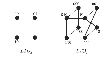
According to Definition 2.1, Figure 1 illustrates and . An alternative definition of is provided in the following non-recursive fashion:
Definition 2.2
[25] Let be a positive integer. The locally twisted cube of dimension has vertices, each labeled by an -bit binary string . Any two nodes and of are adjacent if and only if one of the following conditions is satisfied.
(1) There is an integer , , such that
(a) ,
(b) , and
(c) all the remaining bits of and are identical.
(2) for some and , where .
Now we introduce two models for fault diagnosis.
In the PMC model, all processors in the system under diagnosis can test one another. The set of tests can be represented by a directed graph , in which each vertex represents a processor, and an edge indicates that the processor has tested processor . The outcome of processor testing processor is denoted by , where
where is the set of faulty processors.
In the MM∗ model, a processor executes comparisons for any pair of its neighboring processors. A graph is used to represent a system, where each vertex represents a processor and each edge represents a link. Assign a task to each vertex. The vertex is a comparator of a pair of processors if and . The outcome of this comparison is denoted by , where
where is the set of faulty processors.
The collection of all outcomes is called a syndrome . The diagnosis problem involves using the syndrome to determine the status (faulty or fault free) of each processor in the system. For a given syndrome , a subset is said to be consistent with if the syndrome can be produced from the faulty set . In concrete terms, in the PMC model, is said to be consistent with if the syndrome can be produced from the situation that, for any such that , if and only if . In the MM∗ model, is said to be consistent with if the syndrome can be produced from the situation that, for any and such that , if and only if . Therefore, on the one hand, a faulty set may produce a number of different syndromes. On the other hand, different faulty sets may produce the same syndrome. Define . Two distinct sets , are said to be indistinguishable if ; otherwise, and are said to be distinguishable. We say that is an indistinguishable pair if ; else, is a distinguishable pair.
The following lemmas give necessary and sufficient conditions for a pair of sets to be distinguishable under the PMC model and the MM∗ model.
Lemma 2.3
Lemma 2.4
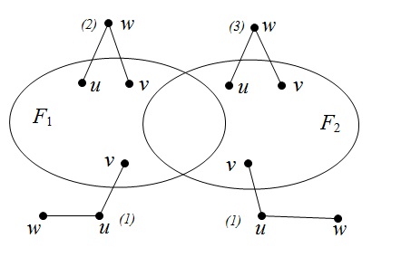
[17] Let be a graph. For any two distinct sets , , and are distinguishable under the MM∗ model if and only if any one of the following conditions is satisfied (See Figure 3 ):
(1) There are two vertices and there is a vertex such that and .
(2) There are two vertices and there is a vertex such that and .
(3) There are two vertices and there is a vertex such that and .
Next, we introduce the diagnosability, conditional diagnosability, -connectivity and -good-neighbor conditional diagnosability of a system in the following statements.
Definition 2.5
[6] A system of processors is -diagnosable if all faulty processors can be detected without replacement, provided that the number of faults does not exceed . The diagnosability of system is the maximum value of such that is -diagnosable.
The diagnosability of multiprocessor systems, as defined above, assumes that all neighbors of any processor may fail simultaneously. However, the probability that all the neighbors of a processor fail is very small. In 2005, Lai et al. [12] introduced conditional diagnosability under the assumption that all the neighbors of any processor in a multiprocessor system cannot be faulty at the same time.
Definition 2.6
[12] System is conditionally -diagnosable if is -diagnosable, provided that for any processor , the set of faults does not contain the neighborhood as a subset. The conditional diagnosability of graph is the maximum value of such that is conditionally -diagnosable.
Inspired by the concept of conditional diagnosability, Peng et al. [15] proposed -good-neighbor conditional diagnosability in 2012, which extended the concept of conditional diagnosability.
Definition 2.7
[15, 28] A faulty set is called a -good-neighbor conditional faulty set if for each node in . A -good-neighbor conditional cut of a graph is a -good-neighbor conditional faulty set such that is disconnected. The minimum cardinality of -good-neighbor cuts is said to be the -connectivity of , denoted by .
Definition 2.8
[15] A system is -good-neighbor conditional -diagnosable if is -diagnosable, provided that every faulty set is a -good-neighbor conditional faulty set. The -good-neighbor conditional diagnosability of is the maximum value of such that is -good-neighbor conditionally -diagnosable.
Thus, the following lemmas give necessary and sufficient conditions for a system to be -good-neighbor -diagnosable under the PMC model and under the MM∗ model.
Lemma 2.9
Lemma 2.10
[6, 28] A system is -good-neighbor -diagnosable under the MM∗ model if and only if each distinct pair of -good-neighbor conditional faulty sets and of with and satisfies one of the following conditions (See Figure 3 ):
(1) There are two vertices and there is a vertex such that and .
(2) There are two vertices and there is a vertex such that and .
(3) There are two vertices and there is a vertex such that and .
Work related to the -connectivity for special networks and small values of can be found in the literature (see, for example, [3, 9, 11, 19, 22, 27]). The following lemmas are very useful for proving our main results.
Lemma 2.11
[15] For any given graph , if , then under the PMC model and MM∗ model.
Lemma 2.12
[21] For any given graph , under the PMC model and MM∗ model.
Lemma 2.13
[7] For any positive integer , there is no cycle of length in the locally twisted cube .
Lemma 2.14
[19] Let be a subgraph of . If , then , where and .
Lemma 2.15
[19] For an -dimensional locally twisted cube , if .
3 Main Results
In this section, we will give the proofs of our main results.
Let and be a positive integer for . Let and be a positive integer for . We use to denote the vertex set
Specifically, we denote the vertex set
by . We can also denote and by and , respectively.
By Lemma 2.12, , where is the classical diagnosability of . We will consider in the following.
First, we consider the upper bound of the -good-neighbor conditional diagnosability of the -dimensional locally twisted cube .
Lemma 3.1
Let and be integers with and . Then, we have under the PMC model and the MM∗ model.
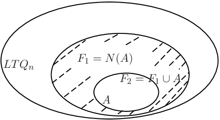
Proof. For , let , , and . By Definition 2.2, we note that
Then, we have , and . Note that and (see Figure 4). Since there is no edge between and , by Lemma 2.3 and Lemma 2.4, we conclude that and are indistinguishable under the PMC model and the MM∗ model.
Now, we verify that both and are -good-neighbor conditional faulty sets.
Suppose . If , then . If , then owing to the fact that and . Thus, has three forms, i.e.,
and
If , then
If , then
If , then
Since is -regular, . Thus, is a -good-neighbor conditional faulty set.
Suppose . If , then we obtain the desired result by the same proof as above. If , then . Note that
Thus, , so is a -good-neighbor conditional faulty set.
By the above discussion, we obtain the result.
Lemma 3.2
Let and be integers with and . Then, we have under the PMC model and the MM∗ model.
Proof. Let and . Then, . Since and , both and are -good-neighbor conditional faulty sets. Note that . Thus, by Definition 2.7, both and are -good-neighbor conditional faulty sets. Since , i.e., , by Lemma 2.3 and Lemma 2.4, and are indistinguishable under the PMC model and the MM∗ model.
Thus, we obtain the result.
Next, we consider the lower bound of the -good-neighbor conditional diagnosability of the -dimensional locally twisted cube under the PMC model and the MM∗ model separately.
Lemma 3.3
Let and be integers with and . Then, we have under the PMC model.
Proof. Suppose that and are any two distinct -good-neighbor conditional faulty sets and they are indistinguishable. We will prove the lemma by showing that or .
If , then , so or for .
Now, we suppose . Since and are indistinguishable, there are no edges between and by Lemma 2.3. Note that and are both -good-neighbor conditional faulty sets. We know that is a -good-neighbor conditional cut. By Lemma 2.15, we obtain that . Since , without loss of generality, we assume that . Since is a -good-neighbor conditional faulty set, any vertex in has at least neighbors in . By Lemma 2.14, we have . Hence, .
This completes the proof of Lemma 3.3.
Lemma 3.4
Let and be integers with and . Then, we have under the MM∗ model.
Proof. Suppose that and are any two distinct -good-neighbor conditional faulty sets and they are indistinguishable. We will prove the lemma by showing that or .
If , then , so or for .
Now, we suppose . Since , without loss of generality, we assume that . To prove this lemma, we consider two cases as follows.
Case 1. .
We shall show that there is no edge between and . Otherwise, there exists an edge , where and . Since is a -good-neighbor conditional faulty set with , has at least two neighbors in . Thus, has a neighbor in or , which contradicts Lemma 2.4. Note that and are -good-neighbor conditional faulty sets. Thus, is a -good-neighbor conditional cut of , so by Lemma 2.15. Since , we have by Lemma 2.14. Therefore, .
Case 2. .
In this case, we have .
If , then .
Now, we suppose . Let be the components of such that , where . For any component , if , then there is no edge between and . Otherwise, it contradicts the fact that and are indistinguishable. Let .
If , then for . Note that and are -good-neighbor conditional faulty sets. Thus, is a -good-neighbor conditional cut of , so by Lemma 2.15. Since , we have . Therefore, .
Next, we assume that . Then, . If , then . The vertex in is one isolated vertex in , which contradicts the fact that is a -good neighbor conditional faulty set. We suppose . Arbitrarily choose a vertex . Then, . Since and are indistinguishable, and by Lemma 2.4. Owing to the fact that and are -good-neighbor conditional faulty sets, we have and . Thus,
It follows that when .
If , then . Thus,
Therefore, for , we have
Now, we assume that . Note that and are -good-neighbor conditional faulty sets. Thus, is a -good-neighbor conditional cut of . By Lemma 2.15, we have . From the assumption that , it follows that . If or , then we have or . Now, assume . Suppose and . Note that each vertex in is adjacent to both and . By the definition of , there are at most two common neighbors for any pair of vertices in , from which it follows that .
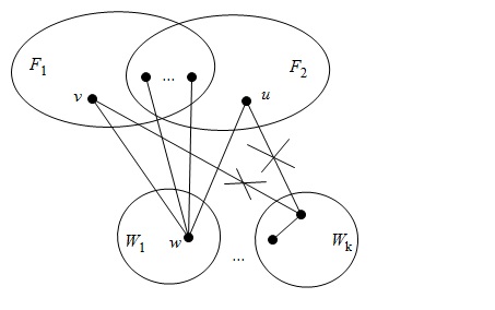
If , suppose that and (see Figure 5). Since contains no triangle by Lemma 2.13, it follows that and . Note that and . By the fact that there is no edge between and when , we have and . By the definition of , there are at most two common neighbors for any pair of vertices in , from which it follows that . Thus,
It follows that for .
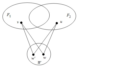
If , suppose that (see Figure 6). Then both and are adjacent to and . Since contains no triangle by Lemma 2.13 and there are at most two common neighbors for any pair of vertices in , we know that the four vertex sets , , and do not pairwise intersect. Therefore,
It follows that for .
The proof of this lemma is complete.
Finally, we give the proofs of our main theorems.
Theorem 3.5
Let be an integer with . Then, the -good-neighbor conditional diagnosability of under the PMC model is
This completes the proof of Theorem 3.5.
Theorem 3.6
Let be an integer with . Then, the -good-neighbor conditional diagnosability of under the MM∗ model is
This completes the proof of Theorem 3.6.
4 Conclusions
In this paper, we determine the -good-neighbor conditional diagnosability of the -dimensional locally twisted cube under the PMC model and the MM∗ model. We show that when , the -good-neighbor conditional diagnosability of under the PMC model is
and when , the -good-neighbor conditional diagnosability of under the MM∗ model is
Future research on this topic will involve studying the -good-neighbor conditional diagnosability of many network topologies.
Acknowledgments
The work is supported by the National Natural Science Foundation of China (11571044, 61373021) and the Fundamental Research Funds for the Central Universities.
References
- [1] J.A. Bondy, U.S.R. Murty, Graph Theory with Applications, The Macmillan Press Ltd, New York, 1976.
- [2] G.Y. Chang, G.H. Chen, G.J. Chang, -diagnosis for matching composition networks under the MM∗ model, IEEE Trans. Comput., 56 (1) (2007), 73–79.
- [3] E. Cheng, L. Lipt k, W. Yang, Z. Zhang, X. Guo, A kind of conditional vertex connectivity of Cayley graphs generated by -trees, Inform. Sci., 181 (19) (2011), 4300–4308.
- [4] C.A. Chen, S.Y. Hsieh, -diagnosis for component-composition graphs under the MM∗ model, IEEE Trans. Comput., 60 (12) (2011), 1704–1717.
- [5] N.W. Chang, S.Y. Hsieh, Structural properties and conditional diagnosability of star graphs by using PMC model, IEEE Trans. Parallel Distrib. Syst., 25 (11) (2014), 3002–3011.
- [6] A.T. Dahbura, G.M. Masson, An faulty identification algorithm for diagnosable systems, IEEE Trans. Comput., 33 (6) (1984), 486–492.
- [7] J. Fan, S. Zhang, X. Jia, G. Zhang, The restricted connectivity of locally twisted cubes, in: Proceeding of International Symposium on Pervasive Systems, Algorithms, and Networks, 2009, pp. 574–578.
- [8] G.H. Hsu, C.F. Chiang, L.M. Shih, L.H. Hsu, J.J.M. Tan, Conditional diagnosability of hypercubes under the comparison diagnosis model, J. Syst. Archit., 55 (2) (2009), 140–146.
- [9] S.Y. Hsieh, H.W. Huang, C.W. Lee, -restricted connectivity of locally twisted cubes, Theor. Comput. Sci., 615 (2016), 78–90.
- [10] S.Y. Hsieh, C.W. Lee, Diagnosability of two-matching composition networks under the MM∗ model, IEEE Trans. Depend. Secure Comput., 8 (2) (2011), 246–255.
- [11] X.J. Li, J.M. Xu, Generalized measures of fault tolerance in exchanged hypercubes, Inform. Process. Lett., 113 (14–16) (2013), 533–537.
- [12] P.L. Lai, J.J.M. Tan, C.P. Chang, L.H. Hsu, Conditional diagnosability measures for large multiprocessor systems, IEEE Trans. Comput., 54 (2) (2005), 165–175.
- [13] L. Lin, L. Xu, D. Wang, S. Zhou, The -Good-Neighbor Conditional Diagnosability of Arrangement Graphs, IEEE Trans. Depend. Secure Comput., DOI: 10.1109/TDSC.2016.2593446.
- [14] J. Maeng, M. Malek, A comparison connection assignment for self-diagnosis of multiprocessor systems, in: Proceeding of 11th International Symposium on Fault-Tolerant Computing, 1981, pp. 173–175.
- [15] S.L. Peng, C.K. Lin, J.J.M. Tan, L.H. Hsu, The -good-neighbor conditional diagnosability of hypercube under the PMC model, Appl. Math. Comput., 218 (21) (2012), 10406–10412.
- [16] F.P. Preparata, G. Metze, R.T. Chien, On the connection assignment problem of diagnosis systems, IEEE Trans. Electron. Comput., EC-16 (6) (1967), 848–854.
- [17] A. Sengupta, A. Dahbura, On self-diagnosable multiprocessor system: diagnosis by the comparison approach, IEEE Trans. Comput., 41 (11) (1992), 1386–1396.
- [18] S. Wang, W. Han, The -good-neighbor conditional diagnosability of -dimensional hypercubes under the MM∗ Model, Inform. Process. Lett., 116 (2016), 574–577.
- [19] C.C. Wei, S.Y. Hsieh, -restricted connectivity of locally twisted cubes, Discrete Appl. Math., 217 (2017), 330–339.
- [20] M. Wang, Y. Liu, S. Wang, The -good-neighbor diagnosability of Cayley graphs generated by transposition trees under the PMC model and MM∗ model, Theor. Comput. Sci., 628 (2016), 92–100.
- [21] M. Wang, Y. Guo, S. Wang, The -good-neighbor diagnosability of Cayley graphs generated by transposition trees under the PMC model and MM∗ model, Int. J. Comput. Math., DOI:10.1080/00207160.2015.1119817.
- [22] M. Wan, Z. Zhang, A kind of conditional vertex connectivity of star graphs, Appl. Math. Lett., 22 (2) (2009), 264–267.
- [23] M. Xu, K. Thulasiraman, X.D. Hu, Conditional diagnosability of matching composition networks under the PMC model, IEEE Trans. Circuits Syst., II, Express Briefs 56 (11) (2009), 875–879.
- [24] M.C. Yang, Conditional diagnosability of matching composition networks under the MM∗ model, Inform. Sci., 233 (1) (2013), 230–243.
- [25] X.F. Yang, G.M. Megson, D.J. Evans, Locally twisted cubes are -pancyclic, Appl. Math. Lett., 17 (2004), 919–925.
- [26] X.F. Yang, D.J. Evans, G.M. Megson, The locally twisted cubes, Int. J. Comput. Math., 82 (4) (2005), 401–413.
- [27] W. Yang, J.X. Meng, Generalized measures of fault tolerance in hypercube networks, Appl. Math. Lett., 25 (10) (2012), 1335–1339.
- [28] J. Yuan, A.X. Liu, X. Ma, X. Qin, J. Zhang, The -good-neighbor conditional diagnosability of -ary -cubes under the PMC model and MM∗ model, IEEE Trans. Parallel Distrib. Syst., 26 (4) (2015), 1165–1177.
- [29] J. Yuan, A. Liu, X. Qin, J. Zhang, J. Li, -good-neighbor conditional diagnosability measures for -ary -cube networks, Theor. Comput. Sci., 626 (2016), 144–162.
- [30] S. Zhou, The conditional diagnosability of crossed cubes under the comparison model, Int. J. Comput. Math., 87 (15) (2010), 3387–3396.
- [31] Q. Zhu, On conditional diagnosability and reliability of the BC networks, J. Supercomput., 45 (2) (2008), 173–184.
- [32] Q. Zhu, S.Y. Liu, M. Xu, On conditional diagnosability of the folded hypercubes, Inform. Sci., 178 (4) (2008), 1069–1077.