Streaming $k$-Means Clustering with Fast Queries

Abstract

We present methods for $k$-means clustering on a stream with a focus on providing fast responses to clustering queries. Compared to the current state-of-the-art, our methods provide substantial improvement in the query time for cluster centers while retaining the desirable properties of provably small approximation error and low space usage. Our algorithms rely on a novel idea of “coreset caching” that systematically reuses coresets (summaries of data) computed for recent queries in answering the current clustering query. We present both theoretical analysis and detailed experiments demonstrating their correctness and efficiency.

1 Introduction

Clustering is a fundamental method for understanding and interpreting data that seeks to partition input objects into groups, known as clusters, such that objects within a cluster are similar to each other, and objects in different clusters are not. A clustering formulation called $k$-means is simple, intuitive, and widely used in practice. Given a set of points $S$ in a Euclidean space and a parameter $k$, the objective of $k$-means is to partition $S$ into $k$ clusters in a way that minimizes the sum of the squared distance from each point to its cluster center.

In many cases, the input data is not available all at once but arrives as a continuous, possibly unending, sequence. This variant, known as streaming $k$-means clustering, requires an algorithm to maintain enough state to be able to incrementally update the clusters as more data arrive. Furthermore, when a query is posed, the algorithm is required to return $k$ cluster centers, one for each cluster, for the data observed so far.

Prior work on streaming $k$-means (e.g. [1, 2, 3, 4]) has mainly focused on optimizing the memory requirements, leading to algorithms with provable approximation quality that only use space polylogarithmic in the input stream’s size [1, 2]. However, these algorithms require an expensive computation to answer a query for cluster centers. This can be a serious problem for applications that need answers in (near) real-time, such as in network monitoring and sensor data analysis. Our work aims at improving the clustering query-time while keeping other desirable properties of current algorithms.

To understand why current solutions to streaming $k$-means clustering have a high query runtime, let us review the framework they use. At a high level, an incoming data stream ${\cal S}$ is divided into smaller “chunks” ${\cal S}_{1},{\cal S}_{2},\ldots,$. Each chunk is summarized into a compact representation, known as a “coreset” (for example, see [5]). The resulting coresets may still not all fit into the memory of the processor. Hence, multiple coresets are further merged recursively into higher-level coresets, forming a hierarchy of coresets, or a “coreset tree”. When a query arrives, all active coresets in the coreset tree are merged together, and a clustering algorithm such as $k$-means++ [6] is applied on the result, outputting $k$ cluster centers. The query time is consequently proportional to the number of coresets that need to be merged together. In prior algorithms, the total size of all these coresets could be as large as the whole memory itself, which causes the query time to often be prohibitively high.

1.1 Our Contributions

We present three algorithms (CC, RCC, and OnlineCC) for streaming $k$-means clustering that asymptotically and practically improve upon prior algorithms’ response time of a query while retaining guarantees on memory efficiency and solution quality of the current state-of-the-art. We provide theoretical analysis, as well as extensive empirical evaluation, of the proposed algorithms.

At the heart of our algorithms is the idea of “coreset caching” that to our knowledge, has not been used before in streaming clustering. It works by reusing coresets that have been computed during previous (recent) queries to speedup the computation of a coreset for the current query. In this way, when a query arrives, the algorithm has no need to combine all coresets currently in memory; it only needs to merge a coreset from a recent query (stored in the coreset cache) along with coresets of points that arrived after this query.

Name	Query Cost	Update Cost	Memory Used	Accuracy: Coreset level
	(per point)	(per point)		returned at query
Coreset Tree (CT)	$O\left(\frac{kdm}{q}\cdot\frac{r\log N}{\log r}\right)$	$O(dm)$	$O\left(dm\cdot\frac{r\log N}{\log r}\right)$	$\log N/\log r$
Cached Coreset Tree (CC)	$O\left(\frac{kdm}{q}\cdot r\right)$	$O(dm)$	$O\left(dm\cdot\frac{r\log N}{\log r}\right)$	$2\log N/\log r$
Recursive Cached Coreset Tree (RCC)	$O\left(\frac{kdm}{q}\cdot\log\log N\right)$	$O(dm\log\log N)$	$O(dmN^{1/8})$	$O(1)$
Online Coreset Cache (OnlineCC)	usually $O(1)$ worst case $O\left(\frac{kdm}{q}\cdot r\right)$	$O(dm)$	$O\left(dm\cdot\frac{r\log N}{\log r}\right)$	$2\log N/\log r$

TABLE I: The time and accuracy of different clustering algorithms. For algorithms other than CT, we assume answering queries by using the coreset cache.

Our theoretical results are summarized in Table I. Throughout, let $n$ denote the number of points observed in the stream so far. We measure an algorithm’s performance in terms of both running time (further separated into query and update) and memory consumption. The query cost, stated in terms of $q$, represents the expected amortized cost per input point assuming that the total number of queries does not exceed $n/q$—or that the average interval between queries is $\Omega(q)$. The update cost is the average (i.e., amortized) per-point processing cost, taken over the entire stream. The memory cost is expressed in terms of words assuming that each point is $d$-dimensional and can be stored in $O(d)$ words. Furthermore, let $m$ denote a user-defined parameter that determines the coreset size ($m$ is set independent of $n$ and is often $O(k)$ in practice); $r$ denote a user-defined parameter that sets the merge degree of the coreset tree; and $N=n/m$ be the number of “base buckets.”

In terms of accuracy, each of our algorithms provides a provable $O(\log k)$-approximation to the optimal $k$-means solution—that is, the quality is comparable, up to constants, to what we would obtain if we simply stored all the points so far in memory and ran an (expensive) batch $k$-means++ algorithm at query time. Further scrutiny reveals that for the same target accuracy (holding constants in the big-$O$ fixed), our simplest algorithm “Cached Coreset Tree” (CC) improves the query runtime of a current state-of-the-art, CT, by a factor of $O(\log N)$—at the expense of a (small) constant factor increase in memory usage. If more flexibility in tradeoffs among the parameters is desired, coreset caching can be applied recursively. Using this scheme, the “Recursive Cached Coreset Tree” (RCC) algorithm can be configured so that it has a query runtime that is a factor of $O(r)$ times faster than CT, and yields better solution quality than CT, at the cost of a small polynomial factor increase in memory.

In practice, a simple sequential streaming clustering algorithm, due to MacQueen [7], is known to be fast but lacks good theoretical properties. We derive an algorithm, called OnlineCC, that combines ideas from CC and sequential streaming to further enhance clustering query runtime while keeping the provable clustering quality of RCC and CC.

We also present an extensive empirical study of the proposed algorithms, in comparison to the state-of-the-art $k$-means algorithms, both batch and streaming. The results show that our algorithms yield substantial speedups (5–100x) in query runtime and total time, and match the accuracy of streamkm++ for a broad range of datasets and query arrival frequencies.

1.2 Related Work

When all input is available at the start of computation (batch setting), Lloyd’s algorithm [8], also known as the $k$-means algorithm, is a simple, widely-used algorithm. Although it has no quality guarantees, heuristics such as $k$-means++ [6] can generate a starting configuration such that Llyod’s algorithm will produce provably-good clusters.

In the streaming setting, [7] is the earliest streaming $k$-means method, which maintains the current cluster centers and applies one iteration of Lloyd’s algorithm for every new point received. Because it is fast and simple, this sequential algorithm is commonly used in practice (e.g., Apache Spark mllib [9]). However, it cannot provide any guarantees on the quality [10]. BIRCH [11] is a streaming clustering method based on a data structure called the CF Tree; it produces cluster centers through agglomerative hierarchical clustering on the leaf nodes of the tree. CluStream[12] constructs “microclusters” that summarize subsets of the stream, and further applies a weighted $k$-means algorithm on the microclusters. STREAMLS [3] is a divide-and-conquer method based on repeated application of a bicriteria approximation algorithm for clustering. A similar divide-and-conquer algorithm based on $k$-means++ is presented in [2]. Invariably, these methods have high query-processing cost and are not suitable for applications that require fast query response. In particular, at the time of query, they require merging multiple data structures, followed by an extraction of cluster centers, which is expensive.

Har-Peled and Mazumdar [5] present coresets of size $O(k\varepsilon^{-d}\log n)$ for summarizing $n$ points $k$-means, and also show how to use the merge-and-reduce technique based on the Bentley-Saxe decomposition [13] to derive a small-space streaming algorithm using coresets. Further work [14, 15, 16] reduced the size of a $k$-means coreset to $O(k/\varepsilon^{2})$. A close cousin to ours, streamkm++ [1] (essentially the CT scheme) is a streaming $k$-means clustering algorithm that uses the merge-and-reduce technique along with $k$-means++ to generate a coreset. Our work improves on streamkm++ w.r.t. query runtime.

Roadmap: We present preliminaries in Section 2, background for streaming clustering in Section 3 and then the algorithms CC, RCC, and OnlineCC in Section 4, along with their proofs of correctness and quality guarantees. We then present experimental results in Section 5.

2 Preliminaries and Notation

We work with points from the $d$-dimensional Euclidean space ${\mathbb{R}}^{d}$ for integer $d>0$. Each point is associated with a positive integral weight ($1$ if unspecified). For points $x,y\in{\mathbb{R}}^{d}$, let $D(x,y)=\Arrowvert{x}-{y}\Arrowvert$ denote the Euclidean distance between $x$ and $y$. Extending this notation, the distance from a point $x\in{\mathbb{R}}^{d}$ to a point set $\Psi\subset{\mathbb{R}}^{d}$ is $D(x,\Psi)=\min_{\psi\in\Psi}\Arrowvert{x}-{\psi}\Arrowvert$. In this notation, the $k$-means clustering problem is as follows:

Problem 1 ($k$-means Clustering).

Given a set $P\subseteq{\mathbb{R}}^{d}$ with $n$ points and a weight function $w\!:P\to{\mathbb{Z}}^{+}$, find a point set $\Psi\subseteq{\mathbb{R}}^{d}$, $|\Psi|=k$, that minimizes the objective function

$$\phi_{\Psi}(P)=\sum_{x\in P}w(x)\cdot D^{2}(x,\Psi)=\sum_{x\in P}\min_{\psi\in\Psi}\left(w(x)\cdot{\Arrowvert{x}-{\psi}\Arrowvert}^{2}\right).$$

Streams: A stream ${\cal S}=e_{1},e_{2},\ldots$ is an ordered sequence of points, where $e_{i}$ is the $i$-th point observed by the algorithm. For $t>0$, let ${\cal S}(t)$ denote the first $t$ entries of the stream: $e_{1},e_{2},\ldots,e_{t}$. For $0<i\leq j$, let ${\cal S}(i,j)$ denote the substream $e_{i},e_{i+1},\ldots,e_{j}$. Define $S={\cal S}(1,n)$ be the whole stream observed until $e_{n}$, where $n$ is, as before, the total number of points observed so far.

$k$-means++ Algorithm: Our algorithms rely on a batch algorithm as a subroutine: $k$-means++ algorithm [6], which has the following properties:

Theorem 1 (Theorem 3.1 in [6]).

On an input set of $n$ points $P\subseteq{\mathbb{R}}^{d}$, the $k$-means++ algorithm returns a set $\Psi$ of $k$ centers such that $\mathop{\text{{E}}}\!\left[\phi_{\Psi}(P)\right]\leq 8(\ln k+2)\cdot\phi_{OPT}(P)$ where $\phi_{OPT}(P)$ is the optimal $k$-means clustering cost for $P$. The time complexity of the algorithm is $O(kdn)$.

Coresets and Their Properties: Our clustering method builds on the concept of a coreset, a small-space representation of a weighted point set that (approximately) preserves desirable properties of the original point set. A variant suitable for $k$-means clustering is as follows:

Definition 1 ($k$-means Coreset).

For a weighted point set $P\subseteq{\mathbb{R}}^{d}$, integer $k>0$, and parameter $0<\varepsilon<1$, a weighted set $C\subseteq{\mathbb{R}}^{d}$ is said to be a $(k,\varepsilon)$-coreset of $P$ for the $k$-means metric, if for any set $\Psi$ of $k$ points in ${\mathbb{R}}^{d}$, we have

$$(1-\varepsilon)\cdot\phi_{\Psi}(P)\leq\phi_{\Psi}(C)\leq(1+\varepsilon)\cdot\phi_{\Psi}(P)$$

Throughout, we use the term “coreset” to always refer to a $k$-means coreset. When $k$ is clear from the context, we simply say an $\varepsilon$-coreset. For integer $k>0$, parameter $0<\varepsilon<1$, and weighted point set $P\subseteq{\mathbb{R}}^{d}$, we use the notation $\texttt{coreset}(k,\varepsilon,P)$ to mean a $(k,\varepsilon)$-coreset of $P$. We use the following observations from [5].

Observation 1 ([5]).

If $C_{1}$ and $C_{2}$ are each $(k,\varepsilon)$-coresets for disjoint multi-sets $P_{1}$ and $P_{2}$ respectively, then $C_{1}\cup C_{2}$ is a $(k,\varepsilon)$-coreset for $P_{1}\cup P_{2}$.

Observation 2 ([5]).

Let $k$ be fixed. If $C_{1}$ is $\varepsilon_{1}$-coreset for $C_{2}$, and $C_{2}$ is a $\varepsilon_{2}$-coreset for $P$, then $C_{1}$ is a $((1+\varepsilon_{1})(1+\varepsilon_{2})-1)$-coreset for $P$.

While our algorithms can work with any method for constructing coresets, an algorithm due to  [16] by Feldman, Schimidt and Sohler provides the following guarantees, which is best coreset construction algorithm from our knowledge:

Theorem 2 ([16] Corollary $4.5$).

Given a point set $P$ with $n$ points, there exists an algorithm to compute $\texttt{coreset}(k,\epsilon,P)$ with size $O(k/\epsilon^{2})$. Let the coreset size be denoted by $m$, then the time complexity of constructing the coreset is $O(dnm)$.

3 Streaming Clustering and Coreset Trees

To provide context for how algorithms in this paper will be used, we describe a generic “driver” algorithm for streaming clustering. We also discuss the coreset tree (CT) algorithm. This is both an example of how the driver works with a specific implementation and a quick review of an algorithm from prior work that our algorithms build upon.

1 def $\texttt{StreamCluster-Update}(\mathcal{H},p)$

       $\rhd$  Insert new point $p$ from the stream into $\mathcal{H}$

2       Add $p$ to $\mathcal{H}.C$

3      

4      if $(|\mathcal{H}.C|=m)$ then

5             $\mathcal{H}.\mathcal{D}$.Update($\mathcal{H}.C$)

6             $\mathcal{H}.C\leftarrow\emptyset$

7            

8      

9 def $\texttt{StreamCluster-Query}()$

10       $C_{1}\leftarrow\mathcal{H}.\mathcal{D}.Coreset()$

11       return $\texttt{$k$-means++}(k,C_{1}\cup\mathcal{H}.C)$

12      

Algorithm 1 Stream Clustering Driver

3.1 Driver Algorithm

The “driver” algorithm (presented in Algorithm 1) internally keeps state as an object $\mathcal{H}$. The state $\mathcal{H}$ involves a specific implementation of a clustering data structure $\mathcal{D}$ and an auxiliary point set $C$. The point set $C$ receives every new point from the stream and with maximum capacity $m$. The size $m$ is the coreset size where the value is determined by the coreset construction algorithm. Once the size of $C$ increases to $m$, the $m$ points will be inserted into the clustering data structure $\mathcal{D}$, as well $C$ will be emptied. So $C$ groups arriving points into batches at the granularity of size $m$ and stores the current batch. Subsequent algorithms in this paper, including CT, are implementations for the clustering data structure $\mathcal{D}$.

3.2 CT: $r$-way Merging Coreset Tree

The $r$-way coreset tree (CT) turns a traditional batch algorithm for coreset construction into a streaming algorithm that works in limited space. Although the basic ideas are the same, our description of CT generalizes the coreset tree of Ackermann et al. [1], which is the special case when $r=2$.

The Coreset Tree: A coreset tree $Q$ maintains buckets at multiple levels. The buckets at level $0$ are called base buckets, which contain the original input points. The size of each base bucket is specified by a parameter $m$. Each bucket above that is a coreset summarizing a segment of the stream observed so far. In an $r$-way CT, level $\ell$ has between $0$ and $r-1$ (inclusive) buckets, each is a summary of $r^{\ell}$ base buckets.

Initially, the coreset tree is empty. After observing $n$ points in the stream, there will be $N=\lfloor n/m\rfloor$ base buckets (level 0). Some of these base buckets may have been merged into higher-level buckets. The distribution of buckets across levels obeys the following invariant:

If $N$ is written in base $r$ as $N=(s_{q},s_{q-1},\dots,s_{1},s_{0})_{r}$, with $s_{q}$ being the most significant digit (i.e., $N=\sum_{i=0}^{q}s_{i}r^{i}$), then there are exactly $s_{i}$ buckets in level $i$.

$\rhd$  Input: bucket $b$

1 def $\texttt{CT-Update}(b)$

2       Append $b$ to $Q_{0}$

3       $j\leftarrow 0$

4       while $|Q_{j}|\geq r$ do

5             $U\leftarrow\texttt{coreset}(k,\varepsilon,\cup_{B\in Q_{j}}B)$

6             Append $U$ to $Q_{j+1}$

7             $Q_{j}\leftarrow\emptyset$

8             $j\leftarrow j+1$

9            

10      

$\rhd$  For query method $\texttt{StreamCluster-Query}()$

11 def CT-Coreset ()

12       return $\bigcup_{j}\{\bigcup_{B\in Q_{j}}B\}$

13      

Algorithm 2 Coreset Tree Algorithm

How is a base bucket added? The process to add a base bucket is reminiscent of incrementing a base-$r$ counter by one, where merging is the equivalent of transferring the carry from one column to the next. More specifically, CT maintains a sequence of sequences $\{Q_{j}\}$, where $Q_{j}$ is the buckets at level $j$. To incorporate a new bucket into the coreset tree, CT-Update, presented in Algorithm 2, first adds it at level $0$. When the number of buckets at any level $i$ of the tree reaches $r$, these buckets are merged, using the coreset algorithm, to form a single bucket at level $(i+1)$, and the process is repeated until there are fewer than $r$ buckets at all levels of the tree. An example of how the coreset tree evolves after the addition of base buckets is shown in Figure 1.

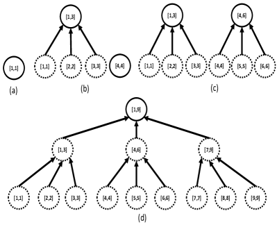
Figure 1: Illustration of a $3$-way coreset tree (CT), showing the states after receiving number of base buckets (a) $1$, (b) $4$, (c) $6$, (d) $9$. The notation $[l,r]$ denotes a coreset of all points in buckets number from $l$ to $r$, both endpoints inclusive. The coreset tree consists of coresets represented by ellipses, each is a base bucket (level $0$) or has been formed by merging multiple coresets from lower levels. A coreset becomes inactive when it is merged and represented by a dotted bordered ellipse.

How to answer a query? The algorithm simply unions all the active buckets together, specifically $\bigcup_{j}\{\bigcup_{B\in Q_{j}}B\}$. Notice that the driver will combine this with a partial base bucket before deriving the $k$-means centers.

Following lemmas stating the properties of the CT algorithm. We use the following definition in proving clustering guarantees.

Definition 2 (Level-$\ell$ Coreset).

For $\ell\in{\mathbb{Z}}_{\geq 0}$, a $(k,\varepsilon,\ell)$-coreset of a point set $P\subseteq{\mathbb{R}}^{d}$, denoted by $\texttt{coreset}(k,\varepsilon,\ell,P)$, is as follows: The level-$0$ coreset of $P$ is $P$. For $\ell>0$, a level-$\ell$ coreset of $P$ is a coreset of the union of $C_{i}$’s (i.e., $\texttt{coreset}(k,\varepsilon,\cup_{i=1}^{t}C_{i})$), where each $C_{i}$ is a level-$\ell_{i}$ coreset, $\ell_{i}<\ell$, of $P_{i}$ such that $\{P_{j}\}_{j=1}^{t}$ forms a partition of $P$.

Lemma 1.

For a point set $P$, parameter $\varepsilon>0$ and integer $\ell\geq 0$, if $C=\texttt{coreset}(k,\varepsilon,\ell,P)$ is a level $\ell$-coreset of $P$, then $C=\texttt{coreset}(k,\varepsilon^{\prime},P)$ where $\varepsilon^{\prime}=\left(1+\varepsilon\right)^{\ell}-1$.

Proof.

We prove this by induction, denote our lemma as proposition $\mathcal{P}$. Consider the base case $\ell=0$, by definition, the level $0$ coreset is in the base buckets where original input points inside, and $\left(1+\epsilon\right)^{0}-1=0$.

Now consider level $\ell>0$. Suppose that $\mathcal{P}(L-1)$ is true, the task is to prove ${\cal P}(L)$. Suppose $C$ is a level $L$ coreset, then $C$ is merged by $r$ level $(L-1)$ coresets. For $i=1\ldots r$, let $C_{i}$ denote the level $(L-1)$ coreset, each summarizing a point set $P_{i}$. Then $C$ must be of the form $C=\texttt{coreset}(k,\epsilon,\cup_{i=1}^{r}C_{i})$.

By the inductive hypothesis, we know that $C_{i}=\texttt{coreset}(k,\epsilon_{i},P_{i})$ where $\epsilon_{i}=\left(1+\epsilon\right)^{L-1}-1$. Let $C^{\prime}=\cup_{i=1}^{r}C_{i}$. From Observation 1 and using $P=\cup_{i=1}^{r}P_{i}$, it must be true that $C^{\prime}=\texttt{coreset}(k,\epsilon_{i},P_{i})$. Since $C=\texttt{coreset}(k,\epsilon,C^{\prime})$ and using Observation 2, we get $C=\texttt{coreset}(k,\gamma,P)$ where $\gamma=(1+\epsilon)(1+\epsilon_{i})-1$. Simplifying, we get $\gamma=(1+\epsilon)(1+\left(1+\epsilon\right)^{(L-1)}-1)-1=\left(1+\epsilon\right)^{L}-1$. This proves the inductive case, which completes the proof.

Fact 1.

After observing $N$ base buckets, the number of levels in the coreset tree CT satisfies $\ell=\max\{j\mid Q_{j}\neq\emptyset\}$, is $\ell\leq\log_{r}N$.

The accuracy of a coreset is given by the following lemma, since it is clear that a level-$\ell$ bucket is a level-$\ell$ coreset of its responsible range of base buckets.

Lemma 2.

Let $\varepsilon=(c\log r)/\log N$ where $c$ is a small enough constant. After observing $N$ base buckets from the stream, a clustering query StreamCluster-Query returns a set of $k$ centers $\Psi$ of $S$ whose clustering cost is a $O(\log k)$-approximation to the optimal clustering for $S$.

Proof.

After observing $N$ base buckets, Fact 1 indicates that all coresets in the coreset tree are at level no greater than $\log_{r}N$. Using Lemma 1, the maximum level coreset is an $\epsilon^{\prime}$-coreset where

$$\epsilon^{\prime}=\left[\left(1+\frac{c\log r}{\log N}\right)^{\frac{\log N}{\log r}}-1\right]\leq\left[e^{\left(\frac{{c}\log r}{\log N}\right)\cdot\frac{\log N}{\log r}}-1\right]<0.1$$

Consider that StreamCluster-Query computes $k$-means++ on the union of two sets, one of the result is CT-Coreset and the other is the partially-filled base bucket $\mathcal{H}.C$. Hence, $\Theta=(\cup_{j}\cup_{B\in Q_{j}}B)\cup\mathcal{H}.C$ is the coreset union that is given to $k$-means++. Using Observation 1, the union set $\Theta$ is a $\epsilon^{\prime}$-coreset of $S$. Let $\Psi$ be the final $k$ centers generated by running $k$-means++ on $\Theta$, and let $\Psi_{OPT}$ be the set of $k$ centers which achieves optimal $k$-means clustering cost for $S$. From the definition of coreset, when $\epsilon^{\prime}<0.1$, we have

$$0.9\phi_{\Psi}(S)\leq\phi_{\Psi}(\Theta)\leq 1.1\phi_{\Psi}(S)$$ (1)

$$0.9\phi_{\Psi_{OPT}}(S)\leq\phi_{\Psi_{OPT}}(\Theta)\leq 1.1\phi_{\Psi_{OPT}}(S)$$ (2)

Let $\Psi_{1}$ denote the set of $k$ centers which achieves optimal $k$-means clustering cost for the union coreset set $\Theta$. Using Theorem 1, we have

$$\mathop{\text{{E}}}\!\left[\phi_{\Psi}(\Theta)\right]\leq 8(\ln k+2)\cdot\phi_{\Psi_{1}}(\Theta)$$ (3)

Since $\Psi_{1}$ is the optimal $k$ centers for $\Theta$, we have

$$\phi_{\Psi_{1}}(\Theta)\leq\phi_{\Psi_{OPT}}(\Theta)$$ (4)

Using Equations 2, 3 and 4 we get

$$\mathop{\text{{E}}}\!\left[\phi_{\Psi}(\Theta)\right]\leq 9(\ln k+2)\cdot\phi_{\Psi_{OPT}}(S)$$ (5)

Using Equations 1 and 5,

$$\mathop{\text{{E}}}\!\left[\phi_{\Psi}(S)\right]\leq 10(\ln k+2)\cdot\phi_{\Psi_{OPT}}(S)$$ (6)

We conclude that $\Psi$ is a factor $O(\log k)$ clustering centers of $S$ compared to the optimal.

The following lemma quantifies the memory and time cost of CT.

Lemma 3.

Let $N$ be the number of base buckets observed so far. Algorithm CT, including the driver, takes amortized $O(dm)$ time per point, using $O\left(dm\cdot\frac{r\log N}{\log r}\right)$ memory. The amortized cost of answering a query is $O\left(\frac{kdm}{q}\cdot\frac{r\log N}{\log r}\right)$ per point.

Proof.

First, the cost of arranging $n$ points into level-$0$ buckets is trivially $O(n)$, resulting in $N=n/m$ buckets. For $j\geq 1$, a level-$j$ bucket is created for every $r^{j}$ buckets, so the number of level-$j$ buckets ever created is $N/r^{j}$. Hence, across all levels, the total number of buckets created is $\sum_{j=1}^{\ell}\tfrac{N}{r^{j}}=O(N/r)$. Furthermore, when a bucket is created, CT merges $rm$ points into $m$ points. By Theorem 2, the total cost of creating these buckets is $O(\tfrac{N}{r}\cdot dm^{2}r)=O(dnm)$, hence $O(dm)$ amortized time per point. In terms of space, each level must have fewer than $r$ buckets, each with $m$ points. Therefore, across $\ell\leq\log_{r}N$ levels, the space required is $O(dm\cdot\frac{r\log N}{\log r})$. Finally, when answering a query, the union of all the buckets has at most $O(m\cdot\frac{r\log N}{\log r})$ points, computable in the same time as the size. Therefore, $k$-means++ run on these points plus one base bucket, takes $O(\frac{kdm}{q}\cdot\frac{r\log N}{\log r})$. The amortized bound immediately follows. This proves the theorem.

As evident from the above lemma, answering a query using CT is expensive compared to the cost of adding a point. More precisely, when queries are made rather frequently—every $q$ points, $q<O(k\cdot\frac{r\log N}{\log r})$—the cost of query processing is asymptotically greater than the cost of handling point arrivals. We address this issue in the next section.

4 Clustering Algorithms with Fast Queries

This section describes algorithms for streaming clustering with an emphasis on query time.

4.1 Algorithm CC: Coreset Tree with Caching

The CC algorithm uses the idea of “coreset caching” to speed up query processing by reusing coresets that were constructed during prior queries. In this way, it can avoid merging a large number of coresets at query time. When compared with CT, the CC algorithm is with the same update process (CT-Update), but apply caching coreset during the query.

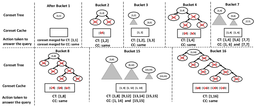
Figure 2: Illustration of Algorithm CC, showing the states of coreset tree and cache after batch $1$, $2$, $3$, $4$, $7$, $8$, $15$ and $16$. The notation $[l,r]$ denotes a coreset of all points in buckets $l$ to $r$, both endpoints inclusive. The coreset tree consists of a set of coresets, each of which is a base bucket or has been formed by merging multiple coresets. Whenever a coreset is merged into a another coreset (in the tree) or discarded (in the cache), the coreset is marked with an “X”. We suppose that a clustering query arrives after seeing each batch, and describe the actions taken to answer this query (1) if only CT was used, or (2) if CC was used along with CT.

In addition to the coreset tree CT, the CC algorithm also has an additional coreset cache denoted by cache, that stores a subset of coresets that were previously computed. When a new query has to be answered, CC avoids the cost of merging coresets from multiple levels in the coreset tree. Instead, it reuses previously cached coresets and retrieves a small number of additional coresets which are the same level of the coreset tree, thus leading to less computation at query time.

However, the level of the resulting coreset increases linearly with the number of merges a coreset is involved in. For instance, suppose we recursively merge the current coreset with the next arriving base bucket of coreset to get a new coreset, and so on, for $N$ batches. The resulting coreset will have a level of $\Theta(N)$, which can lead to a poor clustering accuracy. Additional care is needed to ensure that the level of a coreset is controlled while caching is used.

Details: Each cached coreset is a summary of base buckets $1$ through some number $u$. We call this number $u$ as the right endpoint of the coreset and use it as the key/index into the cache. We call the interval $[1,u]$ as the “span” of the bucket. To explain which coresets can be reused by the algorithm, we introduce the following definitions.

For integers $n>0$ and $r>0$, consider the unique decomposition of $n$ according to powers of $r$ as $n=\sum_{i=0}^{j}\beta_{i}r^{\alpha_{i}}$, where $0\leq\alpha_{0}<\alpha_{1}\ldots<\alpha_{j}$ and $0<\beta_{i}<r$ for each $i$. The $\beta_{i}$s can be viewed as the non-zero digits in the representation of $n$ as a number in base $r$. Let $\texttt{minor}(n,r)=\beta_{0}r^{\alpha_{0}}$, the smallest term in the decomposition, and $\texttt{major}(n,r)=n-\texttt{minor}(n,r)$. Note that when $n$ is in the form of single term $\beta r^{\alpha}$ where $0<\beta<r$ and $\alpha\geq 0$, $\texttt{major}(n)=0$.

For $\kappa=1\ldots j$, let $n_{\kappa}=\sum_{i=\kappa}^{j}\beta_{i}r^{\alpha_{i}}$. $n_{\kappa}$ can be viewed as the number obtained by dropping the $\kappa$ smallest non-zero digits in the representation of $n$ as a number in base $r$. The set $\texttt{prefixsum}(n,r)$ is defined as $\{n_{\kappa}\mid\kappa=1\ldots j\}$. When $n$ is of the form $\beta r^{\alpha}$ where $0<\beta<r$, $\texttt{prefixsum}(n,r)=\emptyset$.

For instance, suppose $n=47$ and $r=3$. Since $47=1\cdot 3^{3}+2\cdot 3^{2}+2\cdot 3^{0}$, we have $\texttt{minor}(47,3)=2,\texttt{major}(47,3)=45$, and $\texttt{prefixsum}(47,3)=\{27,45\}$.

CC caches every coreset whose right endpoint is in $\texttt{prefixsum}(N,r)$. When a query arrives when $N$ buckets received, the task is to compute a coreset whose span is $[1,N]$. CC partitions $[1,N]$ as $[1,N_{1}]\cup[N_{1}+1,N]$ where $N_{1}=\texttt{major}(N,r)$. Out of these two intervals, suppose the query comes after every new base bucket received, this guarantees that $[1,N_{1}]$ should be available in the cache. $[N_{1}+1,N]$ is retrieved from the coreset tree, through the union of no more than $(r-1)$ coresets. This needs a merge of no more than $r$ coresets. This is in contrast with CT, which may need to merge as many as $(r-1)$ coresets at each level of the tree, resulting in a merge of up to $(r-1)\cdot\frac{\log N}{\log r}$ coresets for all levels at query time.

The algorithm for maintaining the cache and answering clustering queries is shown in Algorithm 3. The caching process works along with the query process (CC-Coreset), in a way that making our algorithm be flexible with the queries by users. When the queries are frequent, our algorithm utilizes the cache to provide a faster query speed and a guarantee on the accuracy of clustering result. Otherwise in case of the queries are infrequent, we will show that the time complexity of updating the cache is at the same level of the query process without caching (algorithm CT). This caching design helps the clustering system to adapt in the faces of both burst queries and occasional queries. Figure 2 shows an example of how the CC algorithms updates the cache and answers queries using cached coresets.

Note that to keep the size of the cache small, as new base buckets arrive, CC-Update will ensure that “stale” or unnecessary coresets are removed. The following fact relates to what the cache should store.

1 def $\texttt{CC-Init}(r,k,\varepsilon)$

       $\rhd$  The coreset tree

2       $Q\leftarrow\texttt{CT-Init}{}(r,k,\varepsilon)$

3       $\texttt{cache}\leftarrow\emptyset$

4 def $\texttt{CC-Update}(b,N)$

       $\rhd$  $b$ is a new bucket and $N$ is the number of buckets received so far.

5       $Q.\texttt{CT-Update}(b,N)$

6      

7 def $\texttt{CC-Coreset}()$

       $\rhd$  Return a coreset of points in buckets $1$ till $N$

8       if $N$ exists in cache then

9             return coreset for buckets $[1,N]$ from the cache

10            

11       $N_{1}\leftarrow\texttt{major}(N,r)$ and $N_{2}\leftarrow\texttt{minor}(N,r)$

12       Let $N_{2}=\beta r^{\alpha}$ where $\alpha$ and $\beta<r$ are positive integers

       $\rhd$  coreset for buckets spanning $[1,N_{1}]$ is not in the cache

13       if $N_{1}$ does not exist in cache then

14            $U\leftarrow\texttt{CT-Coreset}()$

15      else

             $\rhd$  $A$ is the coreset for buckets $N_{1}+1,N_{1}+2,\ldots,(N_{1}+N_{2})=N$ and is retrieved from the coreset tree

16             $a\leftarrow\cup_{B\in Q_{\alpha}}B$

             $\rhd$  $b$ is the coreset for buckets spanning $[1,N_{1}]$, retrieved from the cache

17             $b\leftarrow\texttt{cache}.{\tt lookup}(N_{1})$

18             $U\leftarrow a\cup b$

19            

       $\rhd$  Store coreset into cache

20       $C\leftarrow\texttt{coreset}(k,\epsilon,U)$

21       Add coreset $C$ to cache using key $N$

22       Remove each bucket from cache whose key does not appear in $\texttt{prefixsum}(N)\cup\{N\}$

23       return $C$

Algorithm 3 Coreset Tree with Caching

Fact 2.

Let $r\geq 2$. For each $N\in{\mathbb{Z}}^{+}$, $\texttt{prefixsum}(N+1,r)\subseteq\texttt{prefixsum}(N,r)\cup\{N\}$.

Since $\texttt{major}(N,r)\in\texttt{prefixsum}(N,r)$ for each $N$, if the query comes after each new base bucket received, we can always retrieve the bucket with span $[1,\texttt{major}(N,r)]$ from cache.

Lemma 4.

Suppose query comes after receiving each new base bucket. Immediately before base bucket $N$ arrives, each $y\in\texttt{prefixsum}(N,r)$ appears in the key set of cache.

Proof.

Proof is by induction on $N$. The base case $N=1$ is trivially true, since $\texttt{prefixsum}(1,r)$ is empty set. For the inductive step, assume that before bucket $N$ arrives, each $y\in\texttt{prefixsum}(N,r)$ appears in cache. During the query after receiving bucket $N$, we store the coreset whose span is $[1,N]$ to the cache. By Fact 2, we know that $\texttt{prefixsum}(N+1,r)\subseteq\texttt{prefixsum}(N,r)\cup\{N\}$. Using this, every bucket with a right endpoint in $\texttt{prefixsum}(N+1,r)$ is present in cache at the beginning of bucket $(N+1)$ arrives. Hence, the inductive step is proved.

When the queries come less frequent, the cache is less frequently updated as well. Then it can not guarantee that the major is in the cache, that is $N_{1}$ may not exist in the cache. In this case, the CC-Coreset will switch back to the CT-Coreset method in CT. We analyze the time complexity of algorithm CC under the assumption that we can always use cache to accelerate the current query. In practice, we run experiments to show the result of algorithm performance when less frequent queries.

Lemma 5.

When queried after inserting base bucket $N$, Algorithm CC-Coreset returns a coreset whose level in no more than $\left\lceil 2\log_{r}N\right\rceil-1$.

Proof.

Let $\chi(N)$ denote the number of non-zero digits in the representation of $N$ as a number in base $r$. We show that the level of the coreset returned by Algorithm CC-Coreset is no more than $\left\lceil\log_{r}N\right\rceil+\chi(N)-1$. Since $\chi(N)\leq\left\lceil\log_{r}N\right\rceil$, the lemma follows.

The proof is by induction on $\chi(N)$. If $\chi(N)=1$, then $\texttt{major}(N,r)=0$, and the coreset is retrieved directly from the coreset tree $Q$. By Fact 1, each coreset in $Q$ is at a level no more than $\lceil\log_{r}N\rceil$, and the base case follows. Suppose the claim was true for all $N$ such that $\chi(N)=t$. Consider $N$ such that $\chi(N)=(t+1)$. The algorithm computes $N_{1}=\texttt{major}(N,r)$, and retrieves the coreset with span $[1,N_{1}]$ from the cache. Note that $\chi(N_{1})=t$. By the inductive hypothesis, the coreset for span $[1,N_{1}]$ is at a level $\left\lceil\log_{r}N\right\rceil+t-1$. The coresets for span $[N_{1}+1,N]$ are retrieved from the coreset tree; note there are multiple such coresets, but each of them is at a level no more than $\left\lceil\log_{r}N\right\rceil$, using Fact 1. The level of the union coreset for span $[1,N]$ is no more than $\left\lceil\log_{r}N\right\rceil+t$, proving the inductive case.

With the coreset level bounded, we can give the guarantee on the accuracy of clustering centers. Let the accuracy parameter $\varepsilon=\frac{c\log r}{2\log N}$, where $c<\ln{1.1}$.

Lemma 6.

After observing $N$ buckets from the stream, when using clustering data structure CC, Algorithm StreamCluster-Query returns a set of $k$ points whose clustering cost is within a factor of $O(\log k)$ of the optimal $k$-means clustering cost.

Proof.

The proof is similar as Lemma 2. From Lemma 5, we know that the level of a coreset returned is no more than $\left\lceil 2\log_{r}N\right\rceil-1$. Using Lemma 1, the returned coreset, say $C$, is an $\varepsilon^{\prime}$-coreset where $\varepsilon^{\prime}=\left[\left(1+\frac{{c}\log r}{2\log N}\right)^{\frac{2\log N}{\log r}}-1\right]\leq\left[e^{\left(\frac{{c}\log r}{2\log N}\right)\cdot\frac{2\log N}{\log r}}-1\right]<0.1$. Following an argument similar to that of Lemma 2, we arrive at the result.

The following lemma shows the time and space complexity of the cache. We show that the time on updating the cache is at least at the same level of the time of answering a query in Algorithm CT, and can be better to be in linear scale of $r$ instead of $\frac{r\log N}{\log r}$.

Lemma 7.

Algorithm 3 processes a stream of points using amortized time $O(dm)$ per point, using memory of $O\left(dm\cdot\frac{r\log N}{\log r}\right)$. The amortized cost of answering a query is $O\left(\frac{kdm}{q}\cdot r\right)$.

Proof.

The runtime for Algorithm CC-Update  is same as the Algorithm CT-Update. The update time for CC-Update is $O(dm)$ per point.

From Lemma 4, $N_{1}$ is always in the cache. Algorithm CC-Coreset combines no more than $r$ buckets, out of which there is no more than one bucket from the cache, and no more than $(r-1)$ from the coreset tree. From Theorem 2, the time to compute coreset on $O(mr)$ points is $O(dm^{2}r)$, and coreset size $m$ is $O(k)$. The time to compute coreset $C$ is $O(kdmr)$. To compute the $k$ centers from $U$, it is necessary to run $k$-means++ on $O(mr)$ points using time $O(kdmr)$. The amortized query time per point is $O\left(\frac{kdmr}{q}\right)$.

The coreset tree $Q$ uses space $O\left(dm\cdot\frac{r\log N}{\log r}\right)$. After processing bucket $N$, cache only stores those buckets that are corresponding to $\texttt{prefixsum}(N,r)\cup\{N\}$. The number of such buckets possible is $O(\log_{r}N)$, so the space cost of cache is $O(dm\cdot\frac{\log N}{\log r})$. The space complexity follows.

4.2 Algorithm RCC: Recursive Coreset Cache

There are still a few issues with the CC data structure. First, the level of the coreset finally generated is $O(\log_{r}N)$. Since theoretical guarantees on the approximation quality of clustering worsen with the number of levels of the coreset, it is natural to ask if the level can be further reduced to $O(1)$. Moreover, the time taken to process a query is linearly proportional to $r$; we wish to reduce the query time even more. While it is natural to aim to simultaneously reduce the level of the coreset as well as the query time, at first glance, these two goals seem to be inversely related. It seems that if we decreased the level of a coreset (better accuracy), then we will have to increase the merge degree, which would in turn increase the query time. For example, if we set $r=\sqrt{N}$, then the level of the resulting coreset is $O(1)$, but the query time will be $O(\sqrt{N})$.

In the following, we present a solution RCC that uses the idea of coreset caching in a recursive manner to achieve both a low level of the coreset, as well as a small query time. In our approach, we keep the merge degree $r$ in a relatively high value, thus keeping the levels of coresets low. At the same time, we use coreset caching even within a single level of a coreset tree, so that there is no need to merge $r$ coresets at query time. Special care is required for coreset caching in this case, so that the level of the coreset does not increase significantly.

For instance, suppose we built another coreset tree with merge degree $2$ for the $O(r)$ coresets within a single level of the current coreset tree, this would lead to a inner tree with level of $\log r$. At query time, we aggregate $O(\log r)$ coresets from this inner tree, in addition to a coreset from the CC. So, this will lead to a level of $O\left(\max\left\{\frac{\log N}{\log r},\log r\right\}\right)$ and a query time proportional to $O(\log r)$. This is an improvement from the coreset cache, which has a query time proportional to $r$ and a level of $O\left(\frac{\log N}{\log r}\right)$.

We can take this idea further by recursively applying the same idea to the $O(r)$ buckets within a single level of the coreset tree. Instead of having a coreset tree with merge degree $2$, we use a tree with a higher merge degree, and then have a coreset cache for this tree to reduce the query time, and apply this recursively within each tree. This way we can approach the ideal of a small level and a small query time. We are able to achieve interesting tradeoffs, as shown in Table II. To keep the level of the resulting coreset low, along with the coreset cache for each level, we also maintain a list of coresets at each level, like in the CT algorithm. To merge coresets to a higher level, we use the list, rather than the recursive coreset cache.

More specifically, the RCC data structure is defined inductively as follows. For integer $i\geq 0$, the RCC data structure of order $i$ is denoted by $\texttt{RCC}(i)$. $\texttt{RCC}(0)$ is a CC data structure with a merge degree of $r_{0}=2$. For $i>0$, $\texttt{RCC}(i)$ consists of:

• $\texttt{cache}(i)$, a coreset cache storing previous coresets.

• For each level $\ell=0,1,2,\ldots$, there are two structures. One is a list of buckets $L_{\ell}$, similar to the structure $Q_{\ell}$ in a coreset tree. The maximum length of a list is $r_{i}=2^{2^{i}}$. Another is an $\texttt{RCC}_{\ell}$ structure which is a RCC structure of a lower order $(i-1)$, which stores the same information as list $L_{\ell}$, except in a way that can be quickly retrieved during a query.

The main data structure $\mathcal{R}$ is initialized as $\mathcal{R}=\texttt{RCC-Init}(\iota)$, for a parameter $\iota$, to be chosen. Note that $\iota$ is the highest order of the recursive structure. This is also called the “nesting depth” of the structure.

1 $\mathcal{R}.\texttt{order}\leftarrow\iota$, $\mathcal{R}.\texttt{cache}\leftarrow\emptyset$, $\mathcal{R}.r\leftarrow 2^{2^{\iota}}$

2

$\rhd$  $N$ is the number of buckets so far

3 $\mathcal{R}.N\leftarrow 0$

4 foreach $\ell=0,1,2,\ldots$ do

5       $\mathcal{R}.L_{\ell}\leftarrow\emptyset$

6       if $\mathcal{R}.\texttt{order}>0$ then

7            $\mathcal{R}.\texttt{RCC}_{\ell}\leftarrow\mathcal{R}.\texttt{RCC-Init}(\mathcal{R}.\texttt{order}-1)$

8      

9 return $\mathcal{R}$

Algorithm 4 $\mathcal{R}.\texttt{RCC-Init}(\iota)$

$\rhd$  $b$ is a new base bucket

1 $\mathcal{R}.N\leftarrow\mathcal{R}.N+1$

$\rhd$  Insert $b$ into $\mathcal{R}.L_{0}$ and merge if needed

2 Append $b$ to $\mathcal{R}.L_{0}$.

3 if $\mathcal{R}.\texttt{order}>0$ then

4       recursively update $\mathcal{R}.\texttt{RCC}_{0}$ by $\mathcal{R}.\texttt{RCC}_{0}.\texttt{RCC-Update}(b)$

5      

6

$\rhd$  Clear $\mathcal{R}.L$ and RCC if number of buckets reaches $r$

7 $\ell\leftarrow 0$

8 while $(|\mathcal{R}.L_{\ell}|=\mathcal{R}.r)$ do

9       $b^{\prime}\leftarrow\texttt{coreset}(k,\varepsilon,\cup_{B\in\mathcal{R}.L_{\ell}}B)$

10       Append $b^{\prime}$ to $\mathcal{R}.L_{\ell+1}$

11       if $\mathcal{R}.\texttt{order}>0$ then

12            recursively update $\mathcal{R}.\texttt{RCC}_{\ell+1}$ by $\mathcal{R}.\texttt{RCC}_{\ell+1}.\texttt{RCC-Update}(b)$

13      

       $\rhd$  Empty the list of coresets $\mathcal{R}.L$

14       $\mathcal{R}.L_{\ell}\leftarrow\emptyset$

       $\rhd$  Empty the RCC structure

15       if $\mathcal{R}.\texttt{order}>0$ then

16            $\mathcal{R}.\texttt{RCC}_{\ell}\leftarrow\texttt{RCC-Init}(\mathcal{R}.\texttt{order}-1)$

17      

18       $\ell\leftarrow\ell+1$

19      

Algorithm 5 $\mathcal{R}.\texttt{RCC-Update}(b)$

1 $U\leftarrow\emptyset$

2 $N_{1}\leftarrow\texttt{major}(\mathcal{R}.N,\mathcal{R}.r)$

3 if $N_{1}$ does not exist in $\mathcal{R}.\texttt{cache}$ then

4       $U\leftarrow\cup_{\ell}\{\mathcal{R}.\texttt{RCC}_{\ell}.\texttt{RCC-Coreset}()\}$

5      

6else

7       $b_{1}\leftarrow$ retrieve coreset with endpoint $N_{1}$ from $\mathcal{R}.\texttt{cache}$

8       Let $\ell^{*}$ be the lowest numbered non-empty level among $\mathcal{R}.L_{i},i\geq 0$.

       $\rhd$  Apply RCC data structure to retrieve the coresets from level $\ell^{*}$

9       if $\mathcal{R}.\texttt{order}>0$ then

10            $b_{2}\leftarrow\mathcal{R}.\texttt{RCC}_{\ell^{*}}.\texttt{RCC-Coreset}()$

11      else

12            $b_{2}\leftarrow\mathcal{R}.L_{\ell^{*}}$

13       $U\leftarrow b_{1}\cup b_{2}$

14

$\rhd$  Store coreset into cache

15 $b^{\prime}\leftarrow\texttt{coreset}(k,\epsilon,U)$

16 Add $b^{\prime}$ to $\mathcal{R}.\texttt{cache}$ with right endpoint $\mathcal{R}.N$

17 From $\mathcal{R}.\texttt{cache}$, remove all buckets $b^{\prime\prime}$ such that ${\tt right}(b^{\prime\prime})\notin\texttt{prefixsum}(\mathcal{R}.N)\cup\{N\}$

return $b^{\prime}$

Algorithm 6 $\mathcal{R}.\texttt{RCC-Coreset}()$

$\iota$	coreset level	Query cost	update cost	Memory
	at query	(per point)	per point
$\log\log N-3$	$O(1)$	$O\left(\frac{kdm}{q}\log\log N\right)$	$O(dm\log\log N)$	$O\left(dmN^{1/8}\right)$
$\log\log N/2$	$O(\sqrt{\log N})$	$O\left(\frac{kdm}{q}\log\log N\right)$	$O(dm\log\log N)$	$O\left(dm2^{\sqrt{\log N}}\right)$

TABLE II: Possible tradeoffs for the $\texttt{RCC}(\iota)$ algorithm, based on the parameter $\iota$, the nesting depth of the structure.

Lemma 8.

When queried after inserting $N$ buckets, Algorithm 6 using $\texttt{RCC}(\iota)$ returns a coreset whose level is $O\left(\frac{\log N}{2^{\iota}}\right)$. The amortized time cost of answering a clustering query is $O\left(\frac{kdm}{q}\cdot\log\log N\right)$ per point.

Proof.

Algorithm 6 retrieves a few coresets from RCC of different orders. From the outermost structure $\texttt{RCC}(\iota)$, it retrieves one coreset $c$ from $\texttt{cache}(\iota)$. Using an analysis similar to Lemma 5, the level of $b_{1}$ is no more than $\frac{2\log N}{\log r_{\iota}}$.

Note that for $i<\iota$, the maximum number of coresets that will be inserted into $\texttt{RCC}(i)$ is $r_{i+1}=r_{i}^{2}$. The reason is that inserting $r_{i+1}$ buckets into $\texttt{RCC}(i)$ will lead to the corresponding list structure for $\texttt{RCC}(i)$ to become full. At this point, the list and the $\texttt{RCC}(i)$ structure will be emptied out in Algorithm 5. From each recursive call to $\texttt{RCC}(i)$, it can be similarly seen that the level of a coreset retrieved from the cache is at level $\frac{2\log{r_{i}}}{\log r_{i-1}}$, which is $O(1)$. The algorithm returns a coreset formed by the union of all the coresets, followed by a further merge step. Thus, the coreset level is one more than the maximum of the levels of all the coresets returned, which is $O\left(\frac{\log N}{\log r_{\iota}}\right)$.

For the query cost, similar to our analysis in CC, we assume that for each order of $\texttt{RCC}(i)$, we can always use the cache in coreset queries. Comparing to Algorithm CC-Coreset, the minor part of coreset is retrieved from the inner RCC data structure with lower order. Thus, for each order of RCC, the number of coresets merged is $2$. The number of coresets merged at query time is equal to two times the nesting depth of the structure, that is $2\cdot\iota$. The query time equals the cost of running $k$-means++ on the union of all these coresets, for a total time of $O(kdm\log\log N)$. The amortized per-point cost of a query follows.

Lemma 9.

The memory consumed by $\texttt{RCC}(\iota)$ is $O(dmr_{\iota})$. The amortized processing time is $O(dm\log\log N)$ per point.

Proof.

First, as stated in the proof of Lemma 8, in $\texttt{RCC}(i)$ for $i<\iota$, there are at most two level of lists $L_{\ell}$.

We prove by induction on $i$ that $\texttt{RCC}(i)$ has no more than $6r_{i}$ buckets. For the base case, $i=0$, and we have $r_{0}=2$. In this case, $\texttt{RCC}(0)$ has two levels, each with no more than $2$ buckets. So that the total memory is no more than $6$ buckets, due to the lists in two levels, and no more than $2$ buckets in the cache, for a total of $6=3r_{0}<6r_{0}$ buckets. For $i=1$, $r_{1}=4$, the two lists have at most $8$ buckets and cache has no more than $2$ buckets. The recursive structures $\texttt{RCC}(0)$ has $6$ buckets and there are two recursive structures, one for each level. Thus in total $\texttt{RCC}(1)$ has no more than $22$ buckets, which is less than $24=6r_{1}$ buckets.

For the inductive case, consider that $\texttt{RCC}(i)$, the list at each level has no more than $r_{i}$ buckets. The recursive structures $\texttt{RCC}_{\ell}$ within $\texttt{RCC}(i)$ themselves have no more than $6r_{i-1}$ buckets. Adding the constant number of buckets within the cache, we get the total number of buckets within $\texttt{RCC}(i)$ to be $2r_{i}+2\cdot 6r_{i-1}+2=2r_{i}+12\sqrt{r_{i}}+2\leq 6r_{i}$, for $r_{i}\geq 16$, i.e. $i\geq 2$. Thus if $\iota$ is the nesting depth of the structure, the total memory consumed is $O(dmr_{\iota})$, since each bucket requires $O(dm)$ space.

For the updating process time cost, when a bucket is inserted into $\mathcal{R}=\texttt{RCC}(\iota)$, it is added to list $L_{0}$ within $\mathcal{R}$. The cost of maintaining these lists, that is the cost of merging into higher level lists, is amortized $O(dm)$ per point, similar to the analysis in Lemma 7. The bucket is also recursively inserted into a $\texttt{RCC}(\iota-1)$ structure, and a further structure within, and the amortized time for each such structure is $O(dm)$ per point. The total time cost is $O(dm\iota)$ per point which is equal to $O(dm\log\log N)$.

Different tradeoffs are possible by setting $\iota$ to specific values. Some examples are shown in the Table II.

4.3 Online Coreset Cache: a Hybrid of CC and Sequential $k$-means

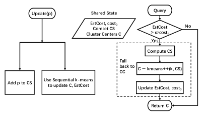
Figure 3: Illustration of Algorithm OnlineCC.

If we break down the query runtime of the algorithms considered so far, we observe two major components: (1) the construction of the coreset of all points seen so far, through merging stored coresets; and (2) the $k$-means++ algorithm applied on the resulting coreset. The focus of the algorithms discussed so far ( CC and RCC) is on decreasing the runtime of the first component, coreset construction, by reducing the number of coresets to be merged at query time. But they still have to pay the cost of the second component $k$-means++, which is substantial in itself, since the runtime of $k$-means++ is $O(kdm)$, where $m$ is the size of the coreset. To make further progress, we have to reduce this component. However, the difficulty in eliminating $k$-means++ at query time is that without an approximation algorithm such as $k$-means++, we have no way to guarantee that the returned clustering is an approximation to the optimal.

This section presents an algorithm, OnlineCC, which only occasionally runs $k$-means++ at query time, and most of the time, uses a much cheaper method that costs $O(1)$ to compute the clustering centers. OnlineCC uses a combination of CC and the Sequential $k$-means algorithm [7] (aka. Online Lloyd’s algorithm) to maintain the cluster centers quickly while also providing a guarantee on the quality of clustering. Like Sequential $k$-means, it incrementall updates the current set of cluster centers for each arriving point. However, while Sequential $k$-means can process incoming points (and answer queries) extremely quickly, it cannot provide any guarantees on the quality of answers, and in some cases, the clustering quality can be very poor when compared with say, $k$-means++. To prevent such deterioration in clustering quality, our algorithm (1) occasionally falls back to CC, which is provably accurate, and (2) runs Sequential $k$-means so long as the clustering cost does not get much larger than the previous time CC was used. This ensures that our clusters always have a provable quality with respect to the optimal.

To accomplish this, OnlineCC also processes incoming points using CC, thus maintaining coresets of substreams of data seen so far. When a query arrives, it typically answers them in $O(1)$ time using the centers maintained using Sequential $k$-means. If, however, the clustering cost is significantly higher (by more than a factor of $\alpha$ for a parameter $\alpha>1$) than the previous time that the algorithm fell back to CC, then the query processing again returns to CC to regenerate a coreset. One difficulty in implementing this idea is that (efficiently) maintaining an estimate of the current clustering cost is not easy, since each change in cluster centers can affect the contribution of a number of points to the clustering cost. To reduce the cost of maintenance, our algorithm keeps an upper bound on the clustering cost; as we show further, this is sufficient to give a provable guarantee on the quality of clustering. Further details on how the upper bound on the clustering cost is maintained, and how algorithms Sequential $k$-means and CC interact are shown in Algorithm 7, with a schematic illustration in Figure 3.

1

2def $\texttt{{OnlineCC}-Init}(k,\varepsilon,\alpha)$

3      

      $\rhd$  $C$ is the current set of cluster centers

4       Initialize $C$ by running $k$-means++ on set ${\cal S}_{0}$ consisting of the first $O(k)$ points of the stream

5      

      $\rhd$  $\phi_{prev}$ is the clustering cost during the previous “fallback” to CC; $\phi_{now}$ is an estimate of the clustering cost of $C$ on the stream so far

6       $\phi_{prev}$, $\phi_{now}$ $\leftarrow$ clustering cost of $C$ on ${\cal S}_{0}$

7       $Q\leftarrow\texttt{CC-Init}(r,k,\varepsilon)$

8      

9

$\rhd$  On receiving a new point $p$ from the stream

10 def $\texttt{{OnlineCC}-Update}(p)$

11       Assign $p$ to the nearest center $c_{p}$ in $C$

12      

13      $\texttt{$\phi_{now}$}\leftarrow\texttt{$\phi_{now}$}+\Arrowvert{p}-{c_{p}}\Arrowvert^{2}$

14      

      $\rhd$  Compute new centroid of $c_{p}$ and $p$ where $w$ is the weight of $c_{p}$

15       $c_{p}^{\prime}\leftarrow(w\cdot c_{p}+p)/(w+1)$

16       Assign the position of $c_{p}^{\prime}$ to $c_{p}$

17       Add $p$ to the current bucket $b$. If $|b|=m$, then $Q.\texttt{CC-Update}(b)$

18      

19

20def $\texttt{{OnlineCC}-Query}()$

21       if $\texttt{$\phi_{now}$}>\alpha\cdot\texttt{$\phi_{prev}$}$ then

22             $CS\leftarrow Q.\texttt{CC-Coreset}()\cup b$, where $b$ is the current bucket that not yet inserted into $Q$

23            

24            $C\leftarrow\texttt{$k$-means++}(k,CS)$

25             $\texttt{$\phi_{prev}$}\leftarrow\phi_{C}(CS)$, the $k$-means cost of coreset $CS$ on centers $C$

26             $\texttt{$\phi_{now}$}\leftarrow\texttt{$\phi_{prev}$}/(1-\varepsilon)$

27            

28       return $C$

29      

Algorithm 7 The Online Coreset Cache: A hybrid of CC and Sequential $k$-means algorithms

Lemma 10.

In Algorithm 7, after observing point set $P$ from the stream, if $C$ is the current set of cluster centers, then $\phi_{now}$ is an upper bound on $\phi_{C}(P)$.

Proof.

Consider the value of $\phi_{now}$ between every two consecutive switches to CC. Without loss of generality, suppose there is one switch happens at time $0$, let $P_{0}$ denote the points observed until time $0$ (including the points received at $0$). We will do induction on the number of points received after time $0$, we denote this number as $i$. Then $P_{i}$ is $P_{0}$ union the $i$ points received after time $0$. Let $\texttt{$\phi_{now}$}(i)$ denote the cost $\phi_{now}$ at time $i$.

When $i$ is $0$, we compute $C$ from the coreset $CS$, from the coreset definition

$$\texttt{$\phi_{prev}$}=\phi_{C}(CS)\geq(1-\epsilon)\cdot\phi_{C}(P_{0})$$

where $\epsilon$ is the approximation factor of coreset $CS$. So for dataset $P_{0}$, the estimation cost $\texttt{$\phi_{now}$}(0)=\texttt{$\phi_{prev}$}/(1-\varepsilon)\geq\phi_{C}(P_{0})$.

At time $i$, denote $C_{i}$ as the cluster centers maintained and $\texttt{$\phi_{now}$}_{i}$ as the estimation of $k$-means cost. Assume the statement is true such that $\texttt{$\phi_{now}$}(i)>\phi_{C_{i}}(P_{i})$.

Consider when a new point $p$ comes, $c_{p}$ is the nearest center in $C_{i}$ to $p$. We compute $c_{p}^{\prime}$, the new position of $c_{p}$, let $C_{i+1}$ denote the new center set where $C_{i+1}=C_{i}\setminus\{c_{p}\}\cup\{c_{p}^{\prime}\}$.

Based on the $\texttt{{OnlineCC}-Update}(p)$ in Algorithm7,

$$\texttt{$\phi_{now}$}(i+1)=\texttt{$\phi_{now}$}(i)+\Arrowvert{p}-{c_{p}}\Arrowvert^{2}$$

From the assumption of inductive step,

$$\texttt{$\phi_{now}$}(i)\geq\phi_{C_{i}}(P_{i})$$

As $c_{p}^{\prime}$ is the centroid of $c_{p}$ and $p$, we have

$$\Arrowvert{p}-{c_{p}}\Arrowvert>\Arrowvert{p}-{c_{p}^{\prime}}\Arrowvert$$

Because $\phi_{C_{i+1}}(P_{i+1})$ is the true cost of point set $P_{i+1}$ on centers $C_{i+1}$,

$$\phi_{C_{i}}(P_{i})+\Arrowvert{p}-{c_{p}^{\prime}}\Arrowvert^{2}\geq\phi_{C_{i+1}}(P_{i+1})$$

Adding up together, we get:

$$\texttt{$\phi_{now}$}(i+1)\geq\phi_{C_{i+1}}(P_{i+1})$$

Thus the inductive step is proved.

Lemma 11.

When queried after observing point set $P$, the OnlineCC algorithm returns a set of $k$ points $C$ whose clustering cost is within $O(\log k)$ of the optimal $k$-means clustering cost of $P$, in expectation.

Proof.

Let $\phi^{*}(P)$ denote the optimal $k$-means cost for $P$. We will show that $\phi_{C}(P)=O(\log k)\cdot\phi^{*}(P)$. There are two cases:

Case I: When $C$ is directly retrieved from CC, Lemma 6 implies that $\mathop{\text{{E}}}\!\left[\phi_{C}(P)\right]\leq O(\log k)\cdot\phi^{*}(P)$. This case is handled through the correctness of CC.

Case II: The query algorithm does not fall back to CC. We first note from Lemma 10 that $\phi_{C}(P)\leq\texttt{$\phi_{now}$}$. Since the algorithm did not fall back to CC, we have $\texttt{$\phi_{now}$}\leq\alpha\cdot\texttt{$\phi_{prev}$}$. Since $\phi_{prev}$ was the result of applying CC to the $P_{0}$ which is the point set received when last recent fall back, we have from Lemma 6 that $\texttt{$\phi_{prev}$}\leq O(\log k)\cdot\phi^{*}(P_{0})$. Since $P_{0}\subseteq P$, we know that $\phi^{*}(P_{0})\leq\phi^{*}(P)$. Putting together the above four inequalities, we have $\phi_{C}(P)=O(\log k)\cdot\phi^{*}(P)$.

5 Experimental Evaluation

This section describes an empirical study of the proposed algorithms, in comparison to the state-of-the-art clustering algorithms. Our goals are twofold: to understand the clustering accuracy and the running time of different algorithms in the context of continuous queries, and to investigate how they behave under different settings of algorithm parameters.

5.1 Datasets

Our experiments use a number of real-world or semi-synthetic datasets, based on data from the UCI Machine Learning Repositories [17]. These are commonly used datasets in benchmarking clustering algorithms. Table III provides an overview of the datasets used.

The Covtype dataset models the forest cover type prediction problem from cartographic variables. The dataset contains $581,012$ instances and $54$ integer attributes. The Power dataset measures electric power consumption in one household with a one-minute sampling rate over a period of almost four years. We remove entries with missing values, resulting in a dataset with $2,049,280$ instances and $7$ floating-point attributes. The Intrusion dataset is a $10\%$-subset of the KDD Cup 1999 data. The task was to build a predictive model capable of distinguishing between normal network connections and intrusions. After ignoring symbolic attributes, we have a dataset with $494,021$ instances and $34$ floating-point attributes. To erase any potential special ordering within data, we randomly shuffle each dataset before using it as a data stream.

However, each of the above datasets, as well as most datasets used in previous works on streaming clustering, is not originally a streaming dataset; the entries are only read in some order and consumed as a stream. To better model the evolving nature of data streams and the drifting of center locations, we generate a semi-synthetic dataset, called Drift, which we derive from the USCensus1990 dataset [17] as follows: The method is inspired by Barddal [18]. The first step is to cluster the USCensus1990 dataset to compute $20$ cluster centers and for each cluster, the standard deviation of the distances to the cluster center. Following that, the synthetic dataset is generated using the Radial Basis Function (RBF) data generator from the MOA stream mining framework [19]. The RBF generator moves the drifting centers with a user-given direction and speed. For each time step, the RBF generator creates $100$ random points around each center using a Gaussian distribution with the cluster standard deviation. In total, the synthetic dataset contains $200,000$ and $68$ floating-point attributes.

Dataset	Number of Points	Dimension	Description
Covtype	$581,012$	$54$	Forest cover type
Power	$2,049,280$	$7$	Household power consumption
Intrusion	$494,021$	$34$	KDD Cup 1999
Drift	$200,000$	$68$	Derived from US Census 1990

TABLE III: An overview of the datasets used in the experiments.

5.2 Experimental Setup and Implementation Details

We implemented all the clustering algorithms in Java, and ran experiments on a desktop with Intel Core i5-4460 $3.2$GHz processor and $8$GB main memory.

Algorithms Implementation: Our baseline algorithms are two prominent streaming clustering algorithms. (1) the Sequential $k$-means algorithm due to MacQueen [7], which is frequently implemented in clustering packages today. For Sequential $k$-means clustering, we use the implementation in Apache Spark MLLib [9], though ours is modified to run sequentially. Furthermore, the initial centers are set by the first $k$ points in the stream instead of setting by random Gaussians, to ensure no clusters are empty. (2) We also implemented streamkm++ [1], a current state-of-the-art algorithm that has good practical performance. streamkm++ can be viewed as a special case of CT where the merge degree $r$ is $2$. The bucket size is $20\cdot k$, where $k$ is the number of centers.

For CC, we set the merge degree to $2$, in line with streamkm++. For RCC, we use a maximum nesting depth of $3$, so the merge degrees for different structures are $N^{\frac{1}{2}},N^{\frac{1}{4}}$ and $N^{\frac{1}{8}}$, respectively. For OnlineCC, the threshold $\alpha$ is set to $1.2$ by default.

We use the batch $k$-means++ algorithm as the baseline for clustering accuracy. This is expected to outperform any streaming algorithm, as with the scope of all the points. The $k$-means++ algorithm, similar to [1, 2], is used to derive coresets. We also use $k$-means++ as the final step to construct $k$ centers from the coreset, and take the best clustering out of five independent runs of $k$-means++; each run of $k$-means++ is followed by up to $20$ iterations of Lloyd’s algorithm to further improve clustering quality. Finally for each statistic, we report the median from nine independent runs of each algorithm to improve robustness. The queries on cluster centers present with interval of $q$ points. Hence, from the beginning of the stream, there is one query per $q$ input points received. By default, the number of clusters is set to $30$, the query interval is set to $100$ points. To present queries in a practical way, we also generate the queries in a poisson process. Let $\lambda$ be the arrival rate of the poisson process, the inter arrival time between query events should be an exponential distribution variable with mean of $1/\lambda$. We set the inter arrival of queries in range of $\{50,100,200,400,800,1600,3200\}$ points.

Metrics: We use three metrics: clustering accuracy, runtime and memory cost. The clustering accuracy is measured using the $k$-means cost, also known as the within cluster sum of squares (SSQ). We measure the average runtime of the algorithm per point, as well as the total runtime over the entire stream. The runtime contains two parts, (1) update time, the time required to update internal data structures upon receiving new point, and (2) query time, the time required to answer clustering queries. Finally, we consider the memory consumption through measuring the number of points stored by the internal data structure, including both the coreset tree and coreset cache. From the number of points, we estimate the number of bytes used, assuming that each dimension of a data point consumes $8$ bytes (size of a double-precision floating-point number).

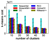
(a) Covtype

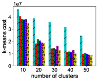
(b) Power

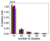
(c) Intrusion ($k$-means cost of Sequential $k$-means is not shown)

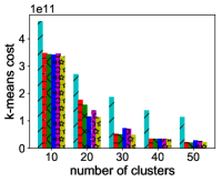
(d) Drift

Figure 4: $k$-means cost vs. number of clusters $k$. The cost is computed at the end of observing all the points. $k$-means cost of Sequential $k$-means on Intrusion dataset is not shown in Figure (c), since it was orders of magnitude larger ($10^{4}$) than the other algorithms.

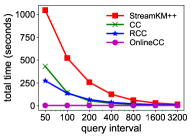
(a) Covtype

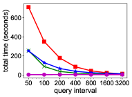
(b) Power

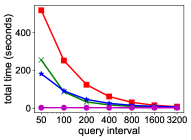
(c) Intrusion

(d) Drift

Figure 5: Total time (seconds) vs. query interval $q$. The total time is for the entire dataset overall stream. For every $q$ points, there is a query for the cluster centers. The number of centers $k$ is $30$.

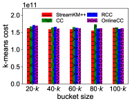
(a) Covtype

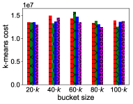
(b) Power

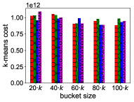
(c) Intrusion

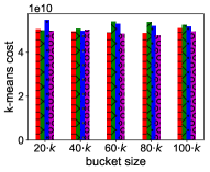
(d) Drift

Figure 6: $k$-means cost vs. bucket size $m$. The cost is computed at the end of observing all the points. The number of clusters $k=30$, query interval $q=100$.

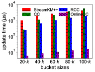
(a) Covtype

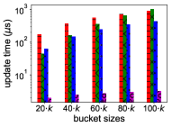
(b) Power

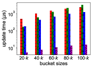
(c) Intrusion

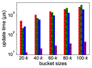
(d) Drift

Figure 7: Average runtime per point (microseconds) vs. bucket size $m$. The runtime is sum of the update time and query time, both counted for average per point. The number of clusters $k=30$, query interval $q=100$.

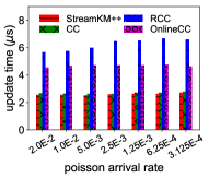
(a) Covtype

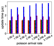
(b) Power

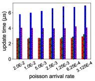
(c) Intrusion

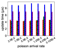
(d) Drift

Figure 8: Update time per point (microseconds) vs. poisson arrival rate $\lambda$.

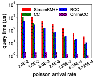
(a) Covtype

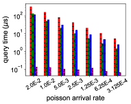
(b) Power

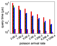
(c) Intrusion

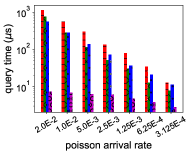
(d) Drift

Figure 9: Query time per point (microseconds) vs. poisson arrival rate $\lambda$.

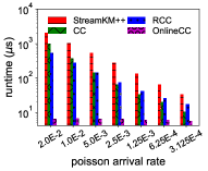
(a) Covtype

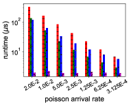
(b) Power

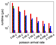
(c) Intrusion

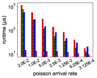
(d) Drift

Figure 10: Total time per point (microseconds) vs. poisson arrival rate $\lambda$.

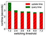
(a) Covtype

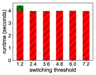
(b) Power

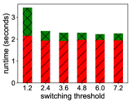
(c) Intrusion

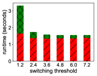
(d) Drift

Figure 11: Total runtime (seconds) vs. switch threshold $\alpha$ in OnlineCC algorithm. The number of clusters $k=30$, query interval $q=100$. The update and query time are both counted for the whole stream instead of per point.

Dataset	Memory cost in points				Memory cost in Megabytes (MB)
	streamkm++	CC	RCC	OnlineCC	streamkm++	CC	RCC	OnlineCC
Covtype	5950	11350	36550	11380	2.57	4.90	15.78	4.92
Power	7150	13750	68950	13780	0.40	0.77	3.86	0.77
Intrusion	5950	11350	32950	11380	1.62	3.09	8.96	3.10
Drift	5350	10150	20950	10180	2.91	5.52	11.40	5.54

TABLE IV: Memory cost of algorithms, number of clusters $k$ is set to $30$ .

5.3 Discussion of Experimental Results

Accuracy ($k$-means cost) vs. $k$: Figures 4 shows the result of $k$-means cost under different number of clusters $k$. Note that for the Intrusion data, the result of Sequential $k$-means is not shown since the cost is much larger (by a factor of about ${10}^{4}$) than the other algorithms. Not surprisingly, for all the algorithms studied, the clustering cost decreases with $k$. For all the datasets, Sequential $k$-means always achieves distinct higher $k$-means cost than other algorithms. This shows that Sequential $k$-means is consistently worse than the other algorithms, when it comes to clustering accuracy—this is as expected, since unlike the other algorithms, Sequential $k$-means does not have a theoretical guarantee on clustering quality.

The other algorithms, streamkm++, CC, RCC, and OnlineCC all achieve very similar clustering cost, on all datasets. In Figure 4, we also show the cost of running a batch algorithm $k$-means++ (followed by Lloyd’s iterations). We found that the clustering costs of the streaming algorithms are nearly the same as that of running the batch algorithm, which can see the input all at once! Indeed, we cannot expect the streaming clustering algorithms to perform any better than this.

Theoretically, it was shown that clustering accuracy improves with the merge degree. Hence, RCC should have the best clustering accuracy (lowest clustering cost). But we do not observe such behaviors experimentally; RCC and streamkm++ show similar accuracy. However their accuracy matches that of batch $k$-means++. A possible reason for this may be that our theoretical analysis of streaming clustering methods is too conservative.

Total Runtime vs. Query Interval: We next consider the effect of different query intervals on the runtime. Figure 5 shows the total runtime throughout the whole stream as a function of the query interval $q$. We note that the total time for OnlineCC is consistently the smallest, and does not change with an increase in $q$. This is because OnlineCC essentially maintains the cluster centers on a continuous basis, while occasionally falling back to CC to recompute coresets, to improve its accuracy. For the other algorithms, including CC, RCC, and streamkm++, the query time and the total time decrease as $q$ increases (and queries become less frequent). CC and RCC have similar total runtime and achieve half of the runtime of streamkm++, by using the cache. All the algorithms converge their total runtime when the queries are very less frequent, that $q$ is more than $1600$ points.

Metrics vs. Bucket Size: We measure the performance of algorithms under different bucket sizes. The bucket size ranges from $20\cdot k$ to $100\cdot k$, where $k$ is the number of clusters and set to $30$. Figure 6 compares the $k$-means cost of different algorithms. The accuracy is similar with different bucket sizes, even though in theory, it should have better accuracy with larger bucket sizes. This observation matches the results in [1], that for most cases in practice, bucket size of $20\cdot k$ is a good number for streamkm++ on clustering accuracy. For our algorithms with coreset caching, the same parameter setting on bucket size applies.

Figure 7 shows the result of average run time per point, which is the sum of both update and query time. Our first observation is that all the timing results are increasing with the bucket size, as both the update and query time are proportional to the bucket size. We also note when bucket size increases over $80\cdot k$, the query time of CC exceeds the query time of streamkm++. The reason is when bucket size increases, the number of buckets received in total becomes smaller and in turn the depth of the coreset tree becomes shorter. Thus for streamkm++, the number of buckets to merge during the query is trivially different than using the cache. Comparing to streamkm++, as CC uses additional time on inserting new coreset to the cache (line $17$ in Algorithm 3), the query time of CC exceeds streamkm++ when bucket size is large.

Queries in Poisson Process: We consider the queries arrive in a poisson process instead of the query interval is in the fixed number of points. The average update time per point, query time per point and total are shown in Figure 8, 9 and 10 respectively, with different value of arrival rate. Note that the higher value of arrival rate, means the less frequent queries. The update time does not have a changing trend with the increasing value of arrival rate, as changing query arrival rate only affects the query process. For all the algorithms, the query time per point drops down with lower arrival rate, as the less frequent queries. Comparing different algorithms, streamkm++ uses most query time without caching. Under high arrival rate $0.02$ such that the average query interval is $50$ points, the query time of RCC is less than CC. When the arrival rate decreases, CC has lower query time. The reason is as follows: generally RCC needs to merge multiple levels of coresets comparing to CC, which only needs to merge one coreset from coreset tree and the other coreset in the cache. However, as RCC applies multiple levels of caches, the chance that successfully finding the target coreset in the cache is much higher than CC. Thus, when queries becomes very frequent, with the help of multiple level of caching, the query time of RCC is faster than CC. Like what we observed in previous experiments, OnlineCC achieves the furthest time in query due to the nature of online cluster centers maintenance. As the query time dominates than the update time, the total runtime per point shown in Figure 10, which is summation of the two, has similar trend as query time per point.

Switching Threshold of OnlineCC: We consider the impact of switching threshold parameter to the OnlineCC algorithm. The runtime throughout the whole stream is shown in Figure 11. From the plot we first observe that runtime decreases with higher value of switching threshold, which indicates the looser requirement on the clustering accuracy. We also notice that the runtime drops dramatically when changing from $1.2$ to $2.4$, approximately $3$ to $5$ times. But much less decrease when the threshold increases further. Thus, the ideal switching threshold value for OnlineCC algorithm is $2$ to $4$ if it has already fulfilled the requirement on accuracy.

Memory Usage: Finally, we report the memory cost in Table IV using $k=30$; the trends are identical for other values of $k$. Evidently, streamkm++ uses the least memory since it only maintains the coreset tree. Because it also maintains a coreset cache, CC requires additional memory. Even then, CC’s memory cost is less than 2x that of streamkm++. The memory cost of OnlineCC is similar to CC while RCC has the highest memory cost. This shows that the marked improvements in speed requires only a modest increase in the memory requirement, making the proposed algorithms practical and appealing.

6 Conclusion

We presented new streaming algorithms for $k$-means clustering. Compared to prior methods, our algorithms significantly speedup query processing, while offering provable guarantees on accuracy and memory cost. The general framework of “coreset caching” may be applicable to other streaming algorithms built around the Bentley-Saxe decomposition. For instance, applying it to streaming $k$-median seems natural. Many other open questions remain, including (1) improved handling of concept drift, through the use of time-decaying weights, and (2) clustering on distributed and parallel streams.

Yu Zhang Yu Zhang is a Ph.D. student in the Department of Electrical and Computer Engineering at Iowa State University. He received his M.S. in Computer Engineering from University of Central Florida in 2012, and his B.S. in Electrical Engineering from University of Science and Technology of China in 2011. He is interested in data stream mining and algorithm design for machine learning.

Kanat Tangwongsan Kanat Tangwongsan is a computer scientist on the faculty of Mahidol University International College. He received his Ph.D. and B.S. in Computer Science from Carnegie Mellon University in 2010 and 2006. He worked at IBM T.J. Watson Research Center as a research staff member from 2010 to 2015. His current research interests are parallel algorithms design for massive data, both in theory and practice.

Srikanta Tirthapura Srikanta Tirthapura is a Professor in the department of Electrical and Computer Engineering at Iowa State University. He received his Ph.D. in Computer Science from Brown University in 2002, and his B.Tech. in Computer Science and Engineering from IIT Madras in 1996. His research interests are algorithm design for big data, including data stream algorithms and parallel and distributed algorithms. He is a recipient of the IBM Faculty Award, and the Warren Boast Award for excellence in Undergraduate Teaching.

References

- [1] M. R. Ackermann, M. Märtens, C. Raupach, K. Swierkot, C. Lammersen, and C. Sohler, “Streamkm++: A clustering algorithm for data streams,” J. Exp. Algorithmics, vol. 17, no. 1, pp. 2.4:2.1–2.4:2.30, 2012.
- [2] N. Ailon, R. Jaiswal, and C. Monteleoni, “Streaming k-means approximation,” in NIPS, 2009, pp. 10–18.
- [3] S. Guha, A. Meyerson, N. Mishra, R. Motwani, and L. O’Callaghan, “Clustering data streams: Theory and practice,” IEEE TKDE, vol. 15, no. 3, pp. 515–528, 2003.
- [4] M. Shindler, A. Wong, and A. Meyerson, “Fast and accurate k-means for large datasets,” in NIPS, 2011, pp. 2375–2383.
- [5] S. Har-Peled and S. Mazumdar, “On coresets for k-means and k-median clustering,” in STOC, 2004, pp. 291–300.
- [6] D. Arthur and S. Vassilvitskii, “k-means++: The advantages of careful seeding,” in SODA, 2007, pp. 1027–1035.
- [7] J. B. MacQueen, “Some methods for classification and analysis of multivariate observations,” in Proc. of the fifth Berkeley Symposium on Mathematical Statistics and Probability, 1967, pp. 281–297.
- [8] S. Lloyd, “Least squares quantization in PCM,” IEEE Trans. Information Theory, vol. 28, no. 2, pp. 129–136, 1982.
- [9] X. Meng, J. K. Bradley, B. Yavuz, and et al., “MLlib: Machine Learning in Apache Spark,” J. Machine Learning Research, vol. 17, pp. 1235–1241, 2016.
- [10] T. Kanungo, D. M. Mount, N. S. Netanyahu, C. D. Piatko, R. Silverman, and A. Y. Wu, “A local search approximation algorithm for k-means clustering,” Computational Geometry, vol. 28, no. 2 - 3, pp. 89 – 112, 2004.
- [11] T. Zhang, R. Ramakrishnan, and M. Livny, “Birch: An efficient data clustering method for very large databases,” in SIGMOD, 1996, pp. 103–114.
- [12] C. C. Aggarwal, J. Han, J. Wang, and P. S. Yu, “A framework for clustering evolving data streams,” in PVLDB, 2003, pp. 81–92.
- [13] J. L. Bentley and J. B. Saxe, “Decomposable searching problems i. static-to-dynamic transformation,” Journal of Algorithms, vol. 1, pp. 301 – 358, 1980.
- [14] S. Har-Peled and A. Kushal, “Smaller coresets for k-median and k-means clustering,” Discrete Computational Geometry, vol. 37, no. 1, pp. 3–19, 2007.
- [15] D. Feldman and M. Langberg, “A unified framework for approximating and clustering data,” in STOC, 2011, pp. 569–578.
- [16] D. Feldman, M. Schmidt, and C. Sohler, “Turning big data into tiny data: Constant-size coresets for k-means, pca and projective clustering,” in SODA, 2013, pp. 1434–1453.
- [17] M. Lichman, “UCI machine learning repository,” 2013. [Online]. Available: http://archive.ics.uci.edu/ml
- [18] J. P. Barddal, H. M. Gomes, F. Enembreck, and J. P. Barthes, “SNCStream+: Extending a high quality true anytime data stream clustering algorithm,” Information Systems, vol. 62, pp. 60 – 73, 2016.
- [19] A. Bifet, G. Holmes, R. Kirkby, and B. Pfahringer, “MOA: Massive Online Analysis,” J. Machine Learning Research, vol. 11, pp. 1601–1604, 2010.