Studying distant galaxies:
A Handbook of Methods and Analyses

F. Hammer¹, M. Puech¹, H. Flores¹, M. Rodrigues¹

¹GEPI, Observatoire de Paris, CNRS, Univ. Paris Diderot, Place Jules Janssen, 92190 Meudon, France

ABSTRACT

Introduction

Galaxies are complex objects comprising hundreds of billions of stars, multiple gas phases, and dust. Present-day galaxies are organized into a well-defined sequence, the Hubble Sequence. Galaxy complexity naturally increases with redshift, since distant galaxies are likely the subject of transformation mechanisms. The study of distant galaxies is particularly enthralling since the Cosmological Principle infers that they are causally linked to the present-day ones.

There are considerable difficulties in studying distant galaxies. The more distant they are, the more they bear witness to the earliest stages of galaxy formation, but this is accompanied by faintness, smallness, and redshifted emissions, all challenges for interpreting their observation. Theoretical interpretations require the determination of stellar and gas mass, star formation, and heavy element abundances, all of which are quantities obtained indirectly, and which are afflicted by uncertainties and systematics both large and numerous. Galaxies are also not homogeneously distributed in space, and their spectral energy distributions are affected by redshift, stellar ages, abundances and dust, thus complicating the rationale of their selection.

This handbook includes a state-of-the-art description of the sampling and selection effects, based on observations with current instruments at large telescopes and using complementary approaches including photometry, imagery, as well as integrated and spatially-resolved spectroscopy. Such methods can be found in a myriad of scientific papers or reviews, synthetized for the first time in a single book. It aims to be a vital tool for teaching final-year undergraduate and postgraduate courses on the topics of “Galaxies” and “Observational Cosmology”. A number of illustrated examples will assist the reader in deriving various galaxy physical quantities from observables. The book shows or proposes numerous methods to derive physical quantities from observations, but also expresses reasonable doubts about far-reaching conclusions made on minimal or insufficient data. Masters and PhD students are encouraged to use it while preparing research projects, including telescope time proposals or articles. Academics may inquire about the numerous aspects surrounding their field of research, which they can better evaluate.

The first chapter establishes how a galaxy sample can be gathered and the many associated caveats which may hamper theoretical interpretations. It addresses the statistical completeness issue, the redshift measurement, the luminosity function analysis, and finally the possibility to causally link galaxy samples from different epochs. The second chapter provides an overview of the basics of imagery and photometry and their uncertainties, as well as the heightened complexity of morphological analyses. A method to derive the latter analyses is proposed, which minimizes systematics while allowing to derive stellar mass and star formation from the energy distribution. The third chapter provides a comprehensive basis for integrated spectroscopy, showing how one can derive the heavy element abundances of their gas phases and star formation rates (SFRs), as well as determine the metal abundances from UV absorption lines and constrain the stellar populations. In principle, velocity is the most directly determined parameter for distant galaxies, and it is the role of Chapter 4 to introduce the considerable limitations caused by galaxy faintness and smallness. It then includes a full description of existing methods for reducing data cubes with a comprehensive treatment of sky residuals, and proposes a method to derive then classify the dynamical state of galaxies, called “morpho-kinematics”. Chapter 5 describes how to synthesize the numerous observations provided for a single, distant galaxy, to determine its physical properties and allow its modeling. It addresses the important question of stellar mass evaluation as well as that of the gas in its various phases. It finally shows the subsequent strengths and weaknesses of scaling relations between mass, velocity, abundance, and star formation.

Chapter 1 Samples and Selection Effects

Here it is an excerpt of Chapter 1.

1 Pre-selection of a sample prior to redshift measurement

Cosmological variance plays an important role in studies of distant galaxies. Variations of the galaxy density are expected at clustering scales of 5 Mpc to 10 Mpc, implying a minimal size of a deep pencil beam of $\sim$100 ${\rm arcmin}^{2}$. Nevertheless, large scale structures like filaments are larger than that and some well-studied fields (e.g., the -South field and the scientific results derived from them may be significantly affected, see (Gilli et al., 2003, Vanzella et al.,2005, Ravikumar et al., 2007).

Typical variations in luminosity density can be up to a factor 2 from one field to another and large scale structures may have a considerably effect on the LF that one derives (see Sec. LABEL:C1_Sect1.3.2 and example therein). This is a strong reason for one to consider more than one field when studying distant galaxies. Generally an uneven number of fields, from 3 to 7 is ideal to perform a redshift survey, allowing a statistically valid check of cosmological variance effects.

1.1 Depth of the photometry and selection effects related to surface-brightness

Galaxies should be selected from a sufficiently deep photometric catalog. The photometric catalog can be tested by the photometric completeness to the deepest counts in the literature. It is generally accepted that the catalog should be complete down to $\sim$1–2 magnitudes fainter than the limit used to perform the galaxy selection in a redshift survey.

Doing otherwise can cause an important fraction of extended sources with relatively low surface brightness to be missed, especially at high redshifts where cosmological dimming effects become very important. Additionally, selecting more distant galaxies is increasingly difficult as they are many more intrinsically faint foreground galaxies (see Sec. LABEL:C1_Sect1.5). These distant galaxies often need photometric and spectroscopic measurements in , which are further affected by surface brightness dimming. The light from extended distant galaxies is affected significantly by cosmological dimming with a factor of $(1+z)^{-4}$ that applies to the surface brightness (bolometric) luminosity of these objects. The strong redshift dependence of this effect can significantly affect the fraction of light detected in the outer isophotes of a galaxy, and can lead to galaxies being excluded from the sample. Cosmological dimming strongly affects extended sources as well as the faint sources at large redshifts. Deep photometry is therefore required to pre-select galaxies in an unbiased way before attempting to determine their redshifts from spectroscopy (see Ex. Photometric depth to recover $z=0.9$ spiral galaxies).

Example 1.1.

Photometric depth to recover $z=0.9$ spiral galaxies Let us assume that most spiral-like galaxies at $z=0.9$ have a central surface brightness similar to that of local spiral galaxies ($\mu_{0}(B)=21.5$). Figure 1 shows that to recover most spiral-like galaxies up to $z\sim 0.9$ in a $I=22.5$ limited sample, it requires a photometry with a completeness up to $I=23.5$. This also implies that detecting lower surface brightness galaxies requires increasingly deeper photometry.

Distant galaxies are forming more stars than present day galaxies and their intrinsic surface-brightness can be expected to be enhanced, making these objects easier to detect. However, the fraction of low surface brightness galaxies in the distant universe is unknown and these objects are most likely to be excluded from a sample. It is therefore crucial to begin by requiring deep photometry as a starting point if one wants to avoid severe biases while selecting a sample of distant galaxies.

Figure 1: Photometry of distant galaxies and related surface brightness selection effects (from the project, (Lilly et al., 1995), ©AAS, reproduced with permission). Left: Number counts of objects with different exposure times. The reached down to $I_{AB}=22.5$ (assumed to be $I_{AB}$, vertical line) and all source counts are complete to this limit, although only 4 h exposure (with ) allow a completeness to $I_{AB}=23.5$ (compare it to the dashed line that represents the deepest counts). Right: Fraction of $I_{AB}=22.5$ galaxies that are recovered by the image detection algorithm, as a function of the central surface brightness. A large exposure time (3–4 h) is necessary to recover $\geq$90% of objects with $\mu(I)=24.5$ that correspond to a face-on, $L*$exponential disk with a scale-length $h=6.6$kpc at $z=0.9$ and with a rest-frame central surface brightness of $\mu_{0}(B)=21.5$.

1.2 Other selection effects$:$ Malmquist bias, Eddington
bias, and lensing effects

There are several gotchas that can negatively affect the quality of a sample of distant galaxies. Even when attempting to select a sample of distant galaxies with a simple criterion, there are several selection effects that can impact scientific results derived from that sample. It is therefore necessary to carefully select the field, the limiting magnitude and the sample size of a survey.

This also implies that one needs to avoid several selection criteria, as the combination of the many related selection effects can be complex and can very severely affect the representativeness and then the whole scientific outputs derived from such a sample.

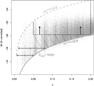
Figure 2: Absolute, $k$-corrected $M_{r}$ magnitudes of galaxies (black points) selected from the survey as a function of redshift (adapted from (Rodrigues et al., 2015). These absolute magnitudes are relatively good proxies for stellar mass. The solid and dashed lines represent the selection with $m_{r}\leq 19.8$ and $\geq$ 14.5, respectively. Selecting $0.05<z<0.2$ galaxies between these two lines would cause an important Malmquist bias, since for example, low luminosity galaxies with $M_{r}\,{>}\,{-}20$ are not detected at $z=0.2$, while they represent most of the sample at $z=0.05$. Avoiding such a bias requires selecting galaxies in the area delineated by the dotted lines (see also the two vertical arrows), which eliminates the low luminosity galaxies lying within the dashed area. The crosses represent two galaxies for which the horizontal, double arrows indicate how $V_{\max}$ can be calculated for establishing the LF (see Sec. LABEL:C1_Sect1.3.2 and Eq. (LABEL:C1_Vmax)).

1.2.1 Malmquist bias

The Malmquist bias is probably the best known selection effect, although it affects all average properties of galaxies, such as the luminosity density, and therefore star formation or stellar density. A survey that is limited by a simple apparent magnitude criterion would be unable to detect intrinsically faint galaxies in its highest redshift bin, while those would be included in the sample in the lower redshift bins. This is illustrated in Fig. 2, which also indicates (see the dotted lines) how to prepare a sample not affected by the Malmquist bias. Neglecting this may lead to significant errors in interpreting, for example, scaling relations (see Chapter 5).

Naturally, calculations of the luminosity density evolution need to be corrected for this effect. At a given redshift bin, one can use the immediately lower redshift bin to evaluate the contribution of the galaxies that have absolute luminosity just below the luminosity cut-off (see, e.g., Lilly et al., 1996). This approach however requires a significant number of galaxies in relatively narrow redshift bins to allow corrections that do not depend too much on evolution.

1.2.2 Eddington bias$:$ magnitude errors near the magnitude limit

Even the most simple and secure case of a magnitude limited sample can be affected by subtle selection effects. For example, consider a sample limited to the magnitude of $m$, and for which the error in measuring the magnitude is $\delta m$. It is often true that the number of fainter galaxies (those with $m+\delta m$) is larger than the number of brighter galaxies with $m-\delta m$. For a random distribution of errors between $\pm$$\delta m$, there will be more sources intrinsically fainter than the limiting magnitude included in the sample than sources intrinsically brighter: this is the Eddington bias. It may seriously affect a sample or a part of a sample where the number count density is very steep. This is the case for example with rare luminous ($L>$) galaxies at the highest redshift bin of a survey, or with any bright sources that are barely detected at large distances.

The Eddington bias can become important when combined with significant photometric errors.

To recover the actual number count, Monte Carlo simulations accounting for the distribution of the noise signal can be compared to the deepest observed counts (see Ex. The Eddington bias for intermediate redshift LIRGs observed by ISO in 1998). This again shows the need for accurate magnitude measurements, especially near the magnitude limit of the galaxy sample.

Example 1.2.

The Eddington bias for intermediate redshift LIRGs observed by ISO in 1998 The satellite detected for the first time the Luminous InfraRed Galaxies ( s) at intermediate redshifts, providing the first estimate of the density evolution of the star formation including both and wavelengths (Flores et al., 1999). However was significantly less sensitive than Spitzer and these s were detected with $\ >4$ and $>3$ for the complementary list. Although s are much more abundant at intermediate $z$ than locally, they are still rare sources and the slope of their number counts, as derived using Spitzer, is $p=1.7$. However number counts from (see Fig. 3) result in a steeper slope of $p=2.3$ because objects with flux below 250 microJy are far more numerous than the brighter ones. This is therefore a good demonstration of the effect of Eddington bias.

Figure 3: The number counts of sources with ${\rm S}/{\rm N}>3$ are shown by the histogram. The dashed line corresponds to a slope $p=2.3$ $(n\sim f_{\nu}^{-p})$ fitting approximately the observed counts. However, deeper observations showed that the slope should be $p=1.7$ (solid line). This effect is due to the Eddington bias, and approximately 25% of the sources in this histogram are almost certainly below the ISO delection limit (250 microJy) and have included into the sample as a result of their large flux calculations errors (from Flores et al., 1999).

1.2.3 Effect of gravitational lensing near the magnitude limit

Gravitational lensing can also cause a somewhat similar selection bias when a galaxy sample is obtained near the line-of-sight of a mass density such as a galaxy cluster or a super-cluster.

Gravitational lensing affects the observed sources density since it causes a brightening of background sources by $\delta\log(f_{\nu})=\log({\rm magnification})$ (or $\delta m=-2.5\times\log({\rm magnification})$) while reducing the area behind the lens due to the convergence of the light beam by a factor equals to $({\rm magnification})^{-1}$. This results in a factor of log($n/n_{0})=(p-1)\times\log({\rm magnification})$, where $n$ is the observed galaxy number density, $n_{0}$ is the source density if there were no lensing, and $p$ is the actual slope of the number density counts. As it is the case with the Eddington bias, gravitational lensing especially affects the brightest sources in a sample (or sub-sample) since the latter often shows steep number counts.

1.3 K-correction and choice of the selecting magnitude

Last but not least, the preparation of a redshift survey requires a careful choice of the wavelength at which apparent magnitudes are used to perform the sample selection. As was discussed in Sec. LABEL:C1_Sect1.1.1, the choice of the selecting wavelength $\lambda_{{\rm sel}}$ is crucial to (1) warrant a fair selection of galaxies independently of their rest-frame color properties; (2) to accurately calculate the rest-frame luminosities.

In fact, most redshift surveys have the goal of comparing the properties of distant galaxies at different redshifts within the survey as well as with the properties of nearby galaxies, where optical filters are defined from the $B$ to the $R$ band and also more recently up to the $K$ band.

Let us consider a redshift survey that is limited by a magnitude limit defined by an observed filter centered at $\lambda_{{\rm sel}}$, i.e., including all galaxies with $m_{\lambda_{{\rm sel}}}\leq m^{\max}_{\lambda_{{\rm sel}}}$. For each galaxy in the survey, a common rest-frame absolute magnitude at a reference wavelength, $\lambda_{{\rm ref}}$, can be computed as:

$$M_{\lambda_{{\rm ref}}}=m_{\lambda_{{\rm sel}}}-5\times\log(d_{L}(z))-k,$$ (1)

where $d_{L}(z)$ is the cosmological luminosity distance and $k$ is the $k$-correction. When a source is observed at a redshift $z$ in a filter centered at $\lambda_{{\rm sel}}$, this provides a direct estimate of the rest-frame absolute magnitude at $\lambda_{{\rm sel}}/(1+z)$, a wavelength that is generally different than the desired $\lambda_{{\rm ref}}$ (see Fig. 4).

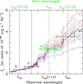
Figure 4: Spectral energy distribution $f_{\nu}$($\lambda$) of a galaxy at $z=0.5$, observed in $B$, V, $I$ broad-band filters (see horizontal solid bars). Fluxes ($f_{\nu}$) can be derived from magnitudes using Eq. (LABEL:C1_AB) and vice-versa. To derive $m^{{\rm rest}}_{\lambda_{{\rm ref}}}$ (here the rest-frame $B$ magnitude at $\lambda_{{\rm ref}}=457$nm, see the green, bold horizontal bar), one needs to adjust the broad-band measurements using a spectrum (here a Sc type at $z=0.5$, see the solid line) extracted from a grid of templates (here with types ranging from Sb to Sd, see red and blue dotted lines). Rest-frame (observed) characteristic wavelengths are indicated on the top (bottom) of the figure, respectively (see also the vertical dot-dash lines). Equation (3) provides directly the $k$-corrected absolute magnitude from $m^{{\rm rest}}_{\lambda_{{\rm ref}}}$.

The $k$-correction $k$ has to be computed to account for this discrepancy. If a galaxy happens to be at a redshift that is exactly $z=\lambda_{{\rm sel}}/\lambda_{{\rm ref}}-1$, one can compute $M_{\lambda_{{\rm ref}}}$ and the $k$-correction is simply $k=-2.5\times\log(1+z)$ to account for the fact that the luminosity $L_{\nu}$ (or the flux $f_{\nu}$ that is related to AB magnitude, see Eq. (LABEL:C1_AB)) is not bolometric but a density per unit frequency (Hogg et al., 2002)

In most cases, however, a priori knowledge of the galaxy spectral energy distribution () is required to compute the $k$-correction. The exact, and complex definition of the $k$-correction can be found in (Hogg et al., 2002).

In practice, an estimate of the $k$-correction can be obtained with a limited knowledge of the that only samples the rest-frame wavelength range from $\lambda_{{\rm ref}}$ to $\lambda_{{\rm sel}}/(1+z)$. Estimating $k$-corrections is simpler if all of the galaxies have actually been observed at $\lambda_{{\rm ref}}$ in addition to $\lambda_{{\rm sel}}$, providing the very useful ($m_{\lambda_{{\rm ref}}}-m_{\lambda_{{\rm sel}}}$) observed color (see Fig. 4). The $k$-correction is then:

$$k=-2.5\times\log(1+z)-(m^{{\rm rest}}_{\lambda_{{\rm ref}}}-m_{\lambda_{{\rm sel}}})$$ (2)

and Eq. (1) simplifies to:

$$M_{\lambda_{{\rm ref}}}=m^{{\rm rest}}_{\lambda_{{\rm ref}}}-5\times\log(d_{L}(z))+2.5\times\log(1+z),$$ (3)

where $m^{{\rm rest}}_{\lambda_{{\rm ref}}}$ is the rest-frame magnitude that the galaxy would have at $\lambda_{{\rm ref}}$ in the rest frame. Figure 4 shows how it can be interpolated from the ($m_{\lambda_{{\rm ref}}}-m_{\lambda_{{\rm sel}}}$) color, which is used to assign an type to each galaxy, using a grid of colors obtained from redshifted galaxy synthesis models.

Other colors can be used to interpolate $m^{{\rm rest}}_{\lambda_{{\rm ref}}}$ and the $k$-correction, but they should be defined over a wavelength range that includes $\lambda_{{\rm ref}}\times(1+z)$. It is however strongly recommended to avoid any extrapolation that can lead to considerable errors in estimating $k$-corrections.

For samples of galaxies spanning a small redshift range, the associated errors can be very small ($\sim$0.05 mag) by setting $\lambda_{{\rm ref}}$ accordingly to the median redshift ($z_{{\rm med}}$), i.e., $\lambda_{{\rm ref}}\sim\lambda_{{\rm sel}}/(1+z_{{\rm med}})$ (Hammer et al., 2001). The calculations of magnitudes, colors and the use of libraries are described in Chapter 2.

Old stellar populations (F, G, and K) have a strong signature at 400nm (the 400nm break) causing a strong decrease in luminosity at $\lambda<400$nm (see Chapter 2). This signature has to be accounted for when defining $\lambda_{{\rm sel}}$ in redshift surveys that aim at comparing distant galaxy properties with the properties of local galaxies. This allows for a better determination of the stellar mass of a galaxy as the galaxy mass can be dominated by old stars emitting most of their light above 400nm rather than by young and blue stars with low $M_{{\rm stellar}}/L$ ratio (see Ex. Selecting wavelength for comparing $z=0$ to $z=0.8$ galaxies).

Example 1.3.

Selecting wavelength for comparing $\bm{z=0}$ to $\bm{z=0.8}$ galaxies Figure 5 compares the $k$-corrections of a survey aiming at characterizing the rest-frame $B$ band properties of galaxies from $z=0$ to 0.8. If galaxies are selected in the observed $B$ band, with increasing redshift this band progressively samples the rest-frame ultraviolet light (see, e.g., Fig. 4). This leads a very wide range of $k$-corrections within the different types, that are up to 4 mag at $z=0.75$. This results in large uncertainties, especially since the properties of the different galaxy types are not very understood in the .

In contrast, a selection in the $I$ band is an exact match to the rest-frame $B$ band at $z=0.82(\lambda_{{\rm ref}}=\lambda_{B}=\lambda_{I}/(1+z)=\lambda_{{\rm sel}}/(1+z))$. The ($B-I$) color (equivalent to the ($m_{\lambda_{{\rm ref}}}-m_{\lambda_{{\rm sel}}}$) color) allows us to interpolate with a far better accuracy and results in much smaller $k$-corrections all the way from $z=0$ to $z=0.82$, because $\lambda_{B}\leq\lambda_{I}/(1+z)\leq\lambda_{I}$. Figure 5 illustrates that by selecting distant galaxies using the apparent $B$ band magnitude, one would exclude elliptical galaxies at high redshift, since these galaxies are made of old and red stellar populations with a low continuum emission in the . The $I$ band selection allows for a much more representative sample of galaxies up to $z=0.82$.

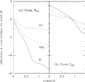
Figure 5: Variations of the $k$-corrections in magnitude (from Lilly et al,., 1995), ©AAS, reproduced with permission) for three types of galaxies, E, Sbc, and Irr, assuming the is computed in absolute magnitude in $B$ band ($\lambda_{{\rm ref}}=457$nm). Left: Assuming that galaxies have been selected from their observed B band magnitudes ($\lambda_{{\rm sel}}=457$nm). Right: Assuming that galaxies have been selected from their observed I band magnitudes ($\lambda_{{\rm sel}}=832$nm).

This further demonstrates how a selection in the $I$ band ($\lambda_{{\rm sel}}=832$nm) is the best way to characterize the rest-frame $B$-band properties for a survey of $z\leq 0.8$ galaxies.

Surveys at $z\leq 2,3$, and 4 require a selection done in the $J$ ($\lambda_{{\rm sel}}=1200$nm), $H$ ($\lambda_{{\rm sel}}=1600$nm) and $K$ ($\lambda_{{\rm sel}}=2100$nm) band, respectively.

When possible, it is even better to select objects in even redder filters to sample the rest-frame properties of galaxies at wavelengths that are not strongly affected by star formation and dust extinction, such as the rest-frame $R,I$, or $K$ bands.

Chapter 2 Imaging and Photometry

Here it is an excerpt of Chapter 2.

2 Galaxy Morphology

2.1 A pragmatic and conservative approach to classify distant galaxies

Classifying the morphology of distant galaxies is usually with the goal to study galaxy evolution. In order to do this, one must assume that distant galaxies are indeed similar to nearby galaxies, i.e., that their morphologies can be characterized using a similar sequence as in the Local Universe. This conservative assumption is the only one allowing to properly calibrate morphological evolution, and has been demonstrated to be robust through comparison with kinematic studies (e.g., Neichel et al., 2008, Hammer et al.,09).

Example 2.1.

How to classify a galaxy morphology using a semi-empirical decision tree?

1. Extract stamp and color images (see Ex. How to construct a color image?) for all galaxies to be classified;

2. Derive $R_{{\rm half}}$ for all galaxies to be classified (see Ex. Measuring the surface brightness profile and basic properties of a distant galaxy);

3. Determine the compactness criterion: there is a limit below which galaxies are too small to be reliably analyzed because of the limited spatial resolution of the images. A strict lowest limit to the half-light radius is given by the size, i.e., $R_{{\rm half}}\sim 0.5\times{\rm FWHM}$. However, because the measurement process of the other steps introduce an additional intrinsic scatter, the real limit is larger. This limit must therefore be derived empirically, by testing the whole decision tree on a test sample. In the case of $z\sim 0.6$ galaxies observed with / images, (Delgado-Serrano et al., 2010) found that this limit is $R_{{\rm half}}\sim 1.33\times{\rm FWHM}=1$ kpc, corresponding to 0.15 arcsec;

4. Isolate compact galaxies in the sample using the compactness criterion;

5. Decompose all of the remaining galaxies into disk and bulge (e.g., using , see Ex. How to fit a galaxy with ?);

6. Assess the bulge/disk decomposition reliability using the residual map and profile cut. Examine whether residuals show asymmetric and/or multiple components (see Fig. 10). Check for off-centered bulges with respect to the disk, i.e., whether the bulge and disk component are consistent;

7. With each reliable fit, derive the $B/T$ flux ratio (e.g., as given by ) and isolate sub-classes depending on the $B/T$ value (see Fig. 10);

8. With each sub-class, examine the color maps to check whether all peculiar sub-structures identified in the residual map and/or stamp image are associated with physically distinct components. In cases of reliable bulge/disk decomposition, check whether a central bulge (if present) is redder than the disk, which is necessary to be able to classify a galaxy as a spiral. This is similar to the appearance of spiral galaxies in the local Universe and ensures that galaxies classified as spirals are indeed comparable in terms of color gradient at any redshift;

9. Based on the result of the last step, assign a final morphological class to the galaxy;

10. Classify the whole sample using at least three different classifiers and compare the results;

11. Repeat the classification until all classifiers agree on the final morphological class, while keeping track of the initial rate of disagreement, which will give an order of estimate of the classification accuracy.

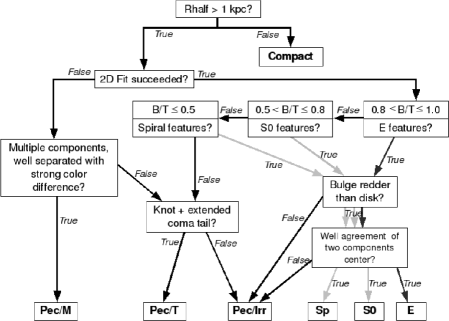
Figure 10: Semi-Empirical morphological classification tree defined by Delgado-Serrano et al. (Delgado-Serrano et al., 2010) to classify the morphology of $z\sim 0.6$ galaxies. Credit: Delgado-Serrano et al., 2010, A&A, 509, 78, reproduced with permission ©ESO.

Such a method was first developed by (Zheng et al., 2004, Zheng et al., 2005, Neichel et al., 2008) for spiral galaxies, and extended by (Delgado-Serrano et al., 2010) to early-type galaxies. It is a semi-empirical method that relies on visual inspection of images using a well defined sequence of procedures in order to limit the subjectivity and improves the reproducibility of the classification. The sequence of procedures is clearly defined and ordered according to a decision tree that must be followed every time a galaxy morphology is being classified (see Ex. How to classify a galaxy morphology using a semi-empirical decision tree?). Specific decision trees must be created based on what observables are available for the classification. As the $B/T$ light ratio is one of the most correlated parameter to the Hubble sequence (e.g., De Lapparent et al., 2011), this parameter should be at the core of any semi-empirical classification, as illustrated inFig. 10.

A decision tree based approach requires the following preliminary steps:

1. Ensure that all images are deep enough to avoid surface brightness effects and sufficiently resolved to limit the fraction of compact galaxies that are not properly resolved;

2. Ensure that all quantities ($B/T$ and $R_{{\rm half}}$) are defined in an optical rest-frame (i.e., at wavelengths larger than $\sim$500nm) as well as the decomposition of the galaxy light profile to estimate residuals, and scale lengths of the bulge and of the disk components;

3. Prepare at least one color map (see Ex. How to construct a color image of a galaxy?).

It is only by combining all these different pieces of information and by comparing the classifications established by three experienced astronomers that one can achieve a robust galaxy morphological classification. Even simpler classifications compared to Fig. 10 can be obtained by merging all peculiar galaxies in a single category, i.e., Peculiar. Indeed, it can be relatively difficult to detect merging features such as tidal tails because they rapidly vanish within less than few hundred years after the merger, they depend on the exact merger orbit, and they correspond to extended and low-surface brightness features strongly affected by cosmological dimming.

The decision tree (see Fig. 10), especially in the simplified form described above, has been shown to lead to a morphological classification that is in good agreement with (1) manual classification made by world experts in galaxy morphology (Van den Bergh 2002) and (2) with a fully independent kinematic classification (Neichel et al., 2008). While the resulting classification is limited by the relatively small size of the sample, it leads to a new and more modern galaxy classification scheme, i.e., a morpho-kinematic classification (Hammer et al., 2009 and see Sec. LABEL:C4_morphokin).

2.1.1 Color maps

Magnitude-scale color-images can be created by combining two images in different bands (Abraham et al., 1999, Menanteau et al., 2001, Zheng et al., 2004). A color image is only useful when the spatial resolution of the original images is similar. Color maps are clearly limited to objects that are properly resolved, i.e., with sizes larger than 2–3 times the size. For distant galaxies, such images should be constructed using space telescope images. Since the integration times of the respective band images are not necessarily the same, a image must also be generated to identify reliable pixels in the color space (see Zheng et al., 2004 and Ex. How to construct a color map of a galaxy?). The advantage of the Zheng et al. (2004) method is that it allows one to also estimate colors in fully extinguished regions. Color maps have a wide range of applications, from pixel-by-pixel analysis (e.g., Abraham et al., 1999, Menanteau et al., 2001, Zibetti et al., 2011), to morphological classification (Zheng et al., 2004; Delgado-Serrano et al., 2010;see Fig. 11).

Example 2.2.

How to construct a color map?

1. Construct two stamp images with the same physical size in the two filters $X$ and $Y$. You will need images that include the sky background. Estimate their spatial resolutions FWHM (see Ex.: How to estimate the spatial resolution of an image?). If for instance the spatial resolution in $X$ is larger than in $Y$, then convolve the $Y$ image using a Gaussian kernel of size $W=\sqrt{{\rm FWHM}_{X}^{2}-{\rm FWHM}_{Y}^{2}}$. The task PSFmatch can be a useful tool for determining the kernel W;

2. Determine the spatial shift and rotation between the two images using at least three stars located as close as possible to the target galaxy and align the two images. Both images should be aligned down to a precision that is smaller than one pixel in both directions;

3. Construct the color map $\mu_{X-Y}$ defined as:

   $$\mu_{X-Y}=-\frac{1}{2}\log{\left(\frac{\sigma^{2}_{X}}{F^{2}_{X}}+1\right)}+\frac{1}{2}\log{\left(\frac{\sigma^{2}_{Y}}{F^{2}_{Y}}+1\right)}+\log{(F_{X}/F_{Y})}$$

   The associated noise within each pixel can be calculated using Eq. (10) of Zheng et al. (2004):

   $$\sigma_{X-Y}^{2}=\log{\left(\frac{\sigma^{2}_{X}}{F^{2}_{X}}+1\right)}+\log{\left(\frac{\sigma^{2}_{Y}}{F^{2}_{Y}}+1\right)}$$

   Here, both the signal and noise include both the source and background. These relation are based on the property that $\sigma_{X}^{2}$ and $\sigma_{Y}^{2}$ are dominated by Poisson noise, which are close to being Log-normal distributions, which therefore allows one to estimate the associated map as $\mu_{X-Y}/\sigma_{X-Y}$.

4. Threshold the color map using a relative threshold in to select reliable pixels, e.g., those with a larger than four times the mean in the background.

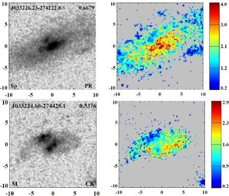
Figure 11: Examples of $B$–$z$ color maps for two $z\sim 0.6$ galaxies from the survey. Credit: Neichel et al. 2008, A&A, 484, 159, reproduced with permission ©ESO. Top panel: J033226.23-274222.8, which was classified as a spiral galaxy. The inner red ellipse corresponds to $\sim R_{{\rm half}}$ with $B-z=2.2$, while the outer blue ellipse corresponds to $\sim 2.R_{{\rm half}}$ with $B-z=1.8$. The $B-z$ color between $R_{{\rm half}}$ and $2.R_{{\rm half}}$ is found to be $\sim$1.5. This difference of color as a function of aperture size, typical of $z\sim 0.6$ spirals (see [Fig. 10] Neichel et al., 2008), can significantly bias the photometric aperture corrections (see Ex. Biases in colors caused by uncontrolled aperture corrections); Bottom panel: J033224.60-274428.1, which was classified as a peculiar galaxy because of the strong color gradient between the two brightest components, which could be indicative of the two progenitors of an on-going merger.

Chapter 3 Integrated Spectroscopy

Here it is an excerpt of Chapter 3.

3 Emission lines

3.1 Proper methods for measuring emission lines

Before measuring the width or flux of the lines, the observed spectrum has to be set to the rest-frame. This can be done by dividing the wavelength scale by $(1+z)$ and multiplying the fluxes $F_{\lambda}$ by $(1+z)$. Notice that $F_{\nu}$ should be divided by $(1+z)$.

At low and moderate resolution, emission lines often display profiles compatible with a Gaussian distribution. The line is measured by fitting a simple Gaussian model. In galaxy spectra, lines lie above the continuum produced by the stars, and a continuum component is added to the Gaussian model, usually a low polynomial order (a constant or a line). The flux of the line is measured by integrating the spectra between $\pm 3\sigma$ of the central wavelength of the fitted Gaussian (see Fig. 14).

For helium and hydrogen recombination lines, such as the Balmer lines, the underlying continuum is more complex because the emission lines are superimposed on the absorption lines produced by the same transition in stellar photospheres (see Fig. 15 and Example Correct from underlying absorption). Not accounting for the underlying absorption when measuring the emission lines leads to the important underestimation of their fluxes and thus induces a bias for all the derived properties (Liang et al., 2004a).

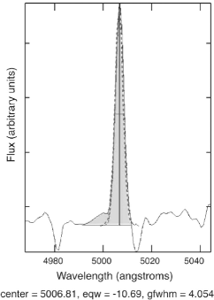
Figure 14: Measure of the [O 3]5007 emission line in a $z=0.6$ galaxy spectrum, using . The line is composed of a main component at the systematic velocity of the galaxy (dashed line), and a blue shifted broad component. The total emission flux from both components can be measured with by integrating the spectra in the vicinity of the two components (filled area).

Example 3.1.

Correcting from underlying
absorption The most efficient method to subtract the stellar component consists in fitting a synthetic spectrum from a template library to the spectrum of each galaxy. The starlight software is taken for illustration but the steps are valid for all full spectrum fitting softwares. For correcting the underlying absorption in Balmer emission lines the steps are:

(1) Adjust the spectral resolution between the templates and the observed spectrum. A majority of softwares automatically match the spectral resolution between the spectral templates and the input spectrum. This works reasonably well in high spectra and when the difference between the two spectral resolution is not too large (Cid Ferandes et al., 2005). However, for in the continuum under ten, it is highly recommended to adjust the template spectral resolution prior to that of the observed spectra, using a Gaussian deconvolution. Always use templates with higher spectral resolution than the observations. Mismatch on the resolution induces bias in the fluxes of Balmer lines.

(2) Mask emission lines in the spectrum to be fitted. Regions associated with emission lines have to be excluded from the fit. In starlight this can be done by setting the weight flag to 0 in the input file. Special attention has to be taken when excluding the emission in Balmer lines: the wings of the absorption line, not contaminated by the emission line, should not be masked since these features give strong constraints on the fit. Strong sky emission or absorption also need to be excluded, see the grey vertical lines in Fig. 15.

(3) Create a library base. The measurement of the fluxes does not strongly depend on the choice of template library. In general, the stellar evolutionary population models are used as base templates in the literature because of their completeness in the $Z$-age grid and their wide wavelength coverage, but empirical stellar or star cluster libraries can also be used. The only requisite is that the templates spectra cover the wavelength range of the input spectrum and that the spectral resolution is higher than the observed spectrum.

(4) Fit and quality control. The fitting algorithm will find the best mix of stellar populations from the template base that adjusts the observed spectrum.The quality of the fit is evaluated by the $\chi^{2}$ value and a visual inspection of critical features, such as the wings of the Balmer lines, the 4000Å, break and the G band, as well as the global slope of the synthetic spectrum. If the slopes of the observed and synthetic spectra do not match, check the spectrophotometric quality of the input spectrum or wherever a nebular continuum should be added in the template base for extremely young objects.

(5) Subtract the synthetic spectrum to the observed spectrum. The synthetic spectrum is subtracted directly to the observed spectrum and emission lines can be measured in the continuum-subtracted spectrum. The continuum of the final spectrum should be flat and close to 0. In particular, check the quality of the fit close to emission lines. A negative continuum means that the absorption lines have been underestimated, while a bump suggests that the underlying absorption has been overestimated. Should one of these problems arise, check that: (a) the spectral resolution has been correctly matched between the observed spectrum and the templates; (b) the Balmer emission lines are correctly masked; (c) if the problem remains this can be due to the template base used, e.g., a young stellar template may be missing.

The estimation of the synthetic spectrum is sensitive to the wavelength window available for the fit. For example, the spectral window between [O 2]$\lambda$3727 and [O 3]$\lambda$5007 has several strong absorption lines (e.g., Balmer lines and Ca lines) and the 4000Å, break, which give strong constraints on the fit. The underlying absorption in Balmer lines can thus be accurately constrained when fitting this wavelength interval.

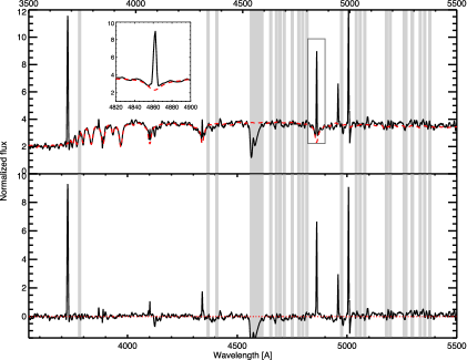
Figure 15: Correcting from underlying absorption in a spectrum of a $z=0.66$ galaxy. Up: The continuum of the rest-frame spectrum (black line) has been fitted using a stellar library and the starlight software. The contribution from the stellar absorption is plotted in red line. The insert box is a zoom on the H$\beta$ line. The emission line and the underlying absorption are clearly visible in the H$\beta$ line. The regions affected by sky lines and the strong O₂ absorption feature from the atmosphere (at 7600Å, in the observed frames) are indicated by grey areas and have been masked during the fit. Down: Final spectrum following subtraction of the stellar continuum, from which the flux of the emission lines can be properly measured.

There are many softwares designed to automatically measure emission lines in large number of spectra and for which the stellar continuum subtraction is included. They are generally based on the assumption that emission lines have simple Gaussian profiles. Since this is not always the case and that at increasing redshifts, galaxies have more complex and disturbed kinematics (Yang et al., 2008), such measurements can lead to systematics ($\sim$10%). Moreover the Poisson noise can affect the profile of faint emission lines, which may become difficult to detect with automatic algorithms. It is thus recommended to manually measure the lines, or at least to manually check the fit accuracy during this process.

3.2 Low S/N regime$:$ measurement bias

In most distant galaxy spectra, some of the diagnostic lines are faint and with low . Here, we show why this problem has to be treated and provide a solution for emission line ratios as well as limits on undetected emissions. The profile signal-to-noise, can be defined as the median in a line:

$${\rm S}/{\rm N}_{{\rm line}}=\frac{F_{{\rm line}}}{\sigma_{c}\times\sqrt{N}},$$ (4)

where $F_{line}$ is the line flux, $\sigma_{c}$ is the noise of the pseudo-continuum, $N$ the number of resolution elements over which the line spreads. If the line has a Gaussian profile, $N$ is equal to six times the emission line width.

The statistical significance is generally evaluated as a function of the equivalent fluctuation of a standard Gaussian stochastic variable. A above 3 implies that the line is detected within a $3\sigma$ significance level, and thus with a probability above 96%. However, the $3\,\sigma$ significance level criterion assumes that the detected signal lies above a known background, affected with pure Gaussian noise. These assumptions are not valid in the case of galaxy spectra, since the continuum is not known a priori, and it is not constant as a function of wavelength due to the underlying stellar populations. Even after subtracting the stellar continuum (see Ex. Correct from underlying absorption), the background still has residual signals arising from uncertainties in the flux calibration and templatesmismatches.

In an ideal case of Poisson noise and a Gaussian line shape with unknown background, Rola et al., (1994) demonstrated that the integrated flux and of a narrow emission line can be described by a lognormal probability distribution. This has a strong impact in the low S/N regime:

The fluxes from lines having observed under 5 are systematically overestimated, because “At very low an emission line can be detected with the help of some chance positive flux fluctuation, but never if it is a negative fluctuation. Most of the time, the observed line intensity is the true line intensity plus a noise intensity under the line, thus the bias”;

Observed over 4–5 (respectively $2\sigma$ and $3\sigma$ confidence level) are required to exclude false detections;

As for color in imagery (see Chapter 2, Sec. 2.1.1), the resulting noise of the logarithm of a line ratio follows a normal distribution (see Appendix in Zheng et al., 2004).

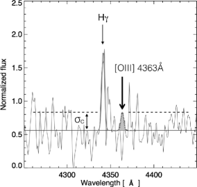
Figure 16: Portion of a spectrum of a $z\sim 0.6$ galaxy, which is shown at rest-frame. The goal is to estimate a limit on the [O iii]$\lambda 4363$Å line while $H\gamma$ is detected and can be used to estimate the expected width of a line (${<}\delta_{v}{>}$). One has to evaluate the noise in the pseudo-continuum ($\sigma_{c}$), and from the Gaussian surface (grey area) one may derive the maximal line flux possessed by a line at 4363Å above the continuum (see the Gaussian with a dotted line) represented by the horizontal full line.

Estimating the upper limit of the flux of an undetected line can be very useful, including to set limits on line flux ratios. Figure 16 shows how this can be done by assuming that the undetected line has a Gaussian line-profile with a width equals to the mean width (${<}\delta_{v}{>}$) of other detected lines, and a height equals to the pseudo-continuum noise $\sigma_{c}$. The line-integrated flux is then $F=\sqrt{2\pi}\cdot\sigma_{c}\cdot\,{<}\delta_{v}{>}$, where $\sqrt{2\pi}$ is coming from the integration of the Gaussian profile, $\sigma_{c}$ is in flux units (either $f_{\nu}$ or $f_{\lambda}$), and ${<}\delta_{v}{>}$ is either in Hertz or Angstrom, respectively.

Chapter 4 Integral Field Spectroscopy

Here it is an excerpt of Chapter 4.

4 Data reduction of IFU observations

4.1 Optimizing sky subtraction with NIR IFUs

In the range, residuals from the subtracted skylines are so intense that they can still affect the detection of target emission lines (see Sec. LABEL:C3_Prepare_Sky). The target has to be carefully chosen in redshift so as to avoid contamination of the galaxy emission lines by strong skylines, otherwise the emission line moments cannot be measured. Figure 15 demonstrates how spatial and temporal variations of the skylines can alter the data and the validity of its reduction and analysis. It is thus mandatory to scrutinize the raw data cube to investigate the presence of undesirable skylines prior to data reduction and analysis.

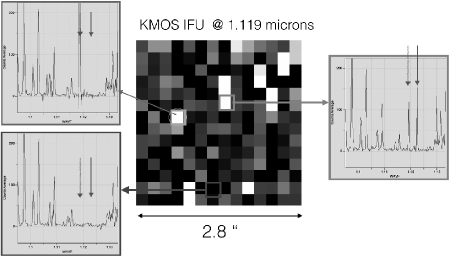
Figure 15: Spatial (and sometimes temporal) variations of the skylines within a data cube. Although the target has been chosen to warrant ${\rm H}\alpha$ in a wavelength range devoid of skylines, their variations at different positions in the jeopardizes the data reduction and analysis if not accounted for. It also evidences the considerable temporal and spatial variations of skylines, which justify favoring instruments with sufficiently high spectral resolution.

The following Ex. Optimizing emission line S/N in the near-IR at moderate resolution presents / J band observations of a $z=0.649$ galaxy. Figure 16 illustrates the considerable gain when properly removing the skyline residuals. Combined with Fig. 15, it demonstrates that an R of 3000 is hardly sufficient to properly remove skylines. This is because such a spectral resolution translates into a velocity resolution of 100 km$s^{-1}$, which corresponds to a significant fraction of the velocity gradient observed in galaxies, especially those observed at moderate inclinations. This can be avoided using resolutions larger than 9000 (see Fig. LABEL:C4_3Dfigfitandres).

Example 4.1.

Optimizing emission line S/N in the near-IR at moderate resolution $($KMOS$)$ Figure 16a shows the spectrum of a spaxel after data reduction: the H$\alpha$ line at 1.082 $\mu$m (in blue) is hardly recognizable within the numerous spikes of sky subtraction residuals. In many spaxels, the of the line is well below the detection threshold if the sky residuals are taken into account in the noise determination. Figure 16b shows the resulting velocity field for such a nonoptimized data reduction. The has to be estimated in a region free of skylines, because sky subtraction residuals artificially enhance the noise which then result in underestimated s. The three-steps procedure to properly estimate the is as follows:

(1) Extracting the mean spectrum of the data cube and create a mask of the wavelength ranges affected by sky residuals. Spikes (both positive and negative) are easy to detect with a peak detection algorithm because they always exhibit the same signature restricted to a single resolution element (see Fig.16a): here, one negative spike followed by a positive spike. Flag the regions to be masked $\sim$ $\pm$ 2 pixels around the spikes.

(2) The masked data cube can then be used to properly estimate the in each spaxel. The data cube can be smoothed spatially using a Gaussian filter of width similar to the of the observations. Spatial smoothing can significantly increase the of the lines at the cost of reducing the spatial resolution of the observation. A Gaussian smoothing should always be applied in the cube after the spikes have been masked out, otherwise the noise would propagate over many pixels in the spectra. Here a Gaussian filter of 1.5 spaxel (0.3 arcsec) in a $3\times 3$ spaxel box has been used for an observational seeing of 0.5 arcsec .

(3) Using the masked and smoothed data cube, the emission line of the object can be fitted with a Gaussian profile to measure the position, width, and flux. The noise is computed from the unmasked pixels on both sides of the line. Figure 16c shows the final velocity field map obtained by using the spatial smoothing and spike rejection algorithms.

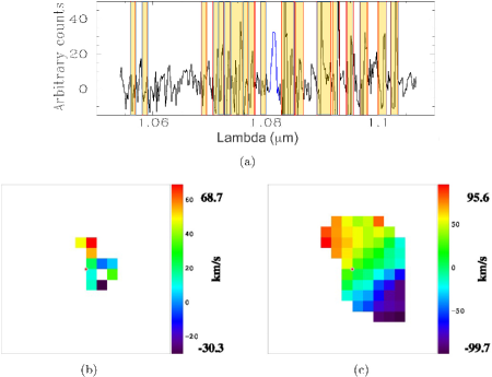
Figure 16: (a) Zoom on a spectrum provided by the sum of sky-subtracted spectra over the spaxels covering a z $=$ 0.649 galaxy. The in the continuum is estimated on a much larger spectral window as provided by . The numerous spikes from sky-residuals are masked (yellow and red vertical lines) within $\pm$2 pixels. (b) Velocity field without masking residual spikes. (c) Same as (b) after masking the skyline residuals and applying a $3\times 3$ Gaussian filter of 1.5 spaxel (0.3 arcsec).

4.2 Measuring emission lines: methods and error budget

The physical and chemical properties of the ionized gas phase in the galaxies may be studied after measuring fluxes, positions, and profile shapes of the most prominent emission lines, such as [O 2]$\lambda\lambda$3726,3729Å, H$\beta$, [O 3]$\lambda\lambda$4959,5007Å, H$\alpha$, [N 2] $\lambda\lambda$6549,6584Å, and [S 2]$\lambda\lambda$6716,6731Å. For a preliminary analysis of a data cube, it is recommended to visualize by eye each individual spectrum to detect possible artifacts or contamination due to sky correction residuals or unexpected faint skylines.

The following example illustrates how errors can be estimated after a Gaussian fit, how they can be optimized in some configurations, and finally how difficult it can be to derive accurate maps of distant galaxy properties. In this case, the presence of gravitational lensing allows robust constraints to be established on the metallicity radial profile for a z $=$ 2.49 source (see Fig. 17). In general, this kind of study can only be achieved for the brightest distant galaxies and only along an average radial profile because of the low in the external regions of the galaxy, and after using Voronoi binning (see Sec. LABEL:C4_spatialsmooth).

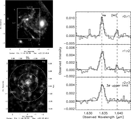
Figure 17: Top-left: F814W and F555W band color image of a galaxy at $z=1.49$, which is gravitationally lensed by the MACS J1149.5+2223 cluster (from Yuan et al., 2011), ©AAS, reproduced with permission). The white rectangular box shows the $4.8\times 6.4$ of the Keck/ . Bottom-left: the detected H$\alpha$ emission from the datacube showing three rings in which the lines are searched. Right: detection in each ring of H$\alpha$ and [N 2]6548-6584 emission lines, allowing one to constrain the metallicity, which decreases from the center to the outskirts.

Example 4.2.

Fitting three lines together Analyses of Keck/ 3D data have used Gaussian profiles to fit three emission lines ([N 2] $\lambda\lambda$6548-6583 and H$\alpha$), simultaneously (Yaun et al., 2011). The search for emission structures with a multiple fit permits the detection of even weak emissions (see Fig. 17). In the , about one out of three lines unavoidably lies near a strong sky line and the procedure needs to take into account the correspondingly higher noise level. The line profile fitting was conducted using a $\chi^{2}$ minimization procedure, and the result can be checked using the fiducial ratio of the [N 2] lines ([N 2]6583/[N 2]$6548=3$). Notice that in this particular example, the is further enhanced by gravitational lensing.

Measurements of emission line fluxes are detailed in Sec. 3.1. Here, we focus on how to measure the centroid and width of the emission lines which are tracing the velocity and velocity dispersion of the gas, respectively.

Measuring these properties requires adequate over a large enough number of resolution elements. The line profile can be defined as the mean value of the flux at a given emission as follows (Flores et al., 2006):

$${\rm S}/{\rm N}=\Sigma^{n}_{i}(S_{i}/(\sqrt{n}\times\sigma_{cont})),$$ (5)

where $n$ is the number of spectral resolution elements in which the emission is detected, $S_{i}$ is the emission line flux at a given voxel $i$, and $\sigma_{cont}$ is the noise measured on the continuum. Only spaxels with sufficient should be considered for further analysis. For a single emission line (e.g., ${\rm H}\alpha$), a $\geq$ 5 should be considered (see Sec. 3.1), while for a doublet such as [O 2], the lower threshold $\geq$ 3 can be considered acceptable (Flores et al., 2006).

At infrared wavelengths, the varies strongly as a function of wavelength due to the numerous skylines (see Fig. LABEL:C4_3Dfigfitandres). The total noise is not only due to the sky background continuum noise but also to the spatial residues of the correction. These originate from spatial and temporal variations of the sky emission lines (see Fig. 15) and further complicate uncertainty estimates. Figure LABEL:C4_3Dfigfitandres further illustrates the need for high spectral resolution in removing faint and narrow skylines that populate spectra at $\lambda>$ 0.72 $\mu$m.

References

- Abraham R. G., Ellis R. S., Fabian A. C. et al. (1999). The star formation history of the hubble sequence: Spatially resolved colour distributions of intermediate-redshift galaxies in the hubble deep field, MNRAS 303, pp. 641–658.
- Cid Fernandes R., Mateus A., Sodré L. et al. (2005). Semi-empirical analysis of sloan digital sky survey galaxies — I. Spectral synthesis method, MNRAS 358, pp. 363–378.
- de Lapparent V., Baillard A., Bertin E. (2011). The EFIGI catalogue of 4458 nearby galaxies with morphology. II. Statistical properties along the Hubble sequence, A&A 532, A75.
- Delgado-Serrano R., Hammer F., Yang Y. B. et al. (2010). How was the hubble sequence 6 gyr ago? A&A 509, A78.
- Flores H., Hammer F., Puech M. et al. (2006). 3D spectroscopy with VLT/GIRAFFE. I. The true Tully Fisher relationship at z 0.6, A&A 455, pp. 107–118.
- Flores H. (1999). Ph.D. thesis, Universit Paris 7 Denis Diderot.
- Gilli R., Cimatti A., Daddi E. et al. (2003). Tracing the large-scale structure in the chandra deep field south, ApJ 592, pp. 721–727.
- Hammer F., Flores H., Puech M. et al. (2009). The hubble sequence: Just a vestige of merger events? A&A 507, pp. 1313–1326.
- Hammer F., Gruel N., Thuan T. X. et al. (2001). Luminous compact galaxies at intermediate redshifts: Progenitors of bulges of massive spirals? ApJ 550, pp. 570–584.
- Hogg D. W., Baldry I. K., Blanton M. R. et al. (2002). The K correction, ArXiv Astrophysics e-prints.
- Liang Y. C., Hammer F., Flores H. et al. (2004). Misleading results from lowres- olution spectroscopy: From galaxy interstellar medium chemistry to cosmic star formation density, A&A 417, pp. 905–918.
- Lilly S. J., Le Fevre O., Hammer F. et al. (1996). The Canada–France redshift survey: The luminosity density and star formation history of the universe to approximately 1, ApJ 460, p. L1.
- Lilly S. J., Le Fevre O., Crampton D. et al. (1995). The Canada–France redshift survey. i. Introduction to the survey, photometric catalogs, and surface brightness selection effects, ApJ 455, p. 50.
- Menanteau F., Jimenez R., Matteucci F. (2001). The origin of blue cores in hubble deep field e/s0 galaxies, ApJ 562, pp. L23–L27.
- Neichel B., Hammer F., Puech M. et al. (2008). Images. ii. a surprisingly low fraction of undisturbed rotating spiral disks at the morpho-kinematical relation 6 gyr ago, A&A 484, pp. 159–172.
- Ravikumar C. D., Puech M., Flores H. et al. (2007). New spectroscopic redshifts from the cdfs and a test of the cosmological relevance of the goods-south field, A&A 465, pp. 1099–1108.
- Rodrigues M., Foster C., Taylor E. et al. (2015). Galaxy And Mass Assembly (GAMA): Chemical evolution of star-forming galaxies from , A&A.
- van den Bergh S. (2002). Ten billion years of galaxy evolution, PASP 114, pp. 797–802.
- Vanzella E., Cristiani S., Dickinson M. et al. (2005). The great observatories origins deep survey. vlt/fors2 spectroscopy in the goods-south field, A&A 434, pp. 53–65.
- Yang Y., Flores H., Hammer F. et al. (2008). IMAGES. I. Strong evolution of galaxy kinematics since , A&A 477, pp. 789–805.
- Yuan T.-T., Kewley L. J., Swinbank A. M. et al. (2011). Metallicity gradient of a lensed face-on spiral galaxy at redshift 1.49, ApJ 732, L14.
- Zheng X. Z., Hammer F., Flores H. et al. (2004). Hst/wfpc2 morphologies and color maps of distant luminous infrared galaxies, A&A 421, pp. 847–862.
- Zibetti S., Groves B. (2011). Resolved optical-infrared spectral energy distributions of galaxies: Universal relations and their break-down on local scales, MNRAS 417, pp. 812–834.